


1. Introduction
The arcsine distribution appears surprisingly in the study of random walks and Brownian motion. Let
 $B\;:\!=\;(B_t; \, t \ge 0)$
be one-dimensional Brownian motion starting at zero. Let
$B\;:\!=\;(B_t; \, t \ge 0)$
be one-dimensional Brownian motion starting at zero. Let
 $G\;:\!=\;\sup\{0 \leq s \leq 1\;:\;B_s = 0\}$
be the last exit time of B from zero before time 1,
$G\;:\!=\;\sup\{0 \leq s \leq 1\;:\;B_s = 0\}$
be the last exit time of B from zero before time 1,
 $G^{\max}\;:\!=\;\inf\{0 \leq s \leq 1\;:\;B_s = \max_{u \in [0,1]} B_{u}\}$
be the first time at which B achieves its maximum on [0,1], and
$G^{\max}\;:\!=\;\inf\{0 \leq s \leq 1\;:\;B_s = \max_{u \in [0,1]} B_{u}\}$
be the first time at which B achieves its maximum on [0,1], and
 $\Gamma\;:\!=\;\int_0^1 1_{\{B_s > 0\}} \, \textrm{d} s$
be the occupation time of B above zero before time 1. In [Reference Lévy43, Reference Lévy44], Lévy proved the celebrated result that G,
$\Gamma\;:\!=\;\int_0^1 1_{\{B_s > 0\}} \, \textrm{d} s$
be the occupation time of B above zero before time 1. In [Reference Lévy43, Reference Lévy44], Lévy proved the celebrated result that G,
 $G^{\max}$
, and
$G^{\max}$
, and
 $\Gamma$
are all arcsine distributed with density
$\Gamma$
are all arcsine distributed with density
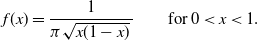 \begin{equation} f(x) = \frac{1}{\pi \sqrt{x(1-x)}\,} \qquad \text{for } 0 < x < 1.\end{equation}
For a random walk
 $S_n\;:\!=\;\sum_{k = 1}^n X_k$
with increments
$S_n\;:\!=\;\sum_{k = 1}^n X_k$
with increments
 $(X_k; \, k \ge 1)$
starting at
$(X_k; \, k \ge 1)$
starting at
 $S_0\;:\!=\;0$
, the counterparts of G,
$S_0\;:\!=\;0$
, the counterparts of G,
 $G^{\max}$
, and
$G^{\max}$
, and
 $\Gamma$
are given by
$\Gamma$
are given by
 $G_n\;:\!=\;\max\{0 \le k \le n: S_k = 0\}$
, the index at which the walk last hits zero before time n,
$G_n\;:\!=\;\max\{0 \le k \le n: S_k = 0\}$
, the index at which the walk last hits zero before time n,
 $G^{\max}_n \;:\!=\;\min\{0 \le k \le n: S_k = \max_{0 \le k \le n}S_k\}$
, the index at which the walk first attains its maximum value before time n,
$G^{\max}_n \;:\!=\;\min\{0 \le k \le n: S_k = \max_{0 \le k \le n}S_k\}$
, the index at which the walk first attains its maximum value before time n,
 $\Gamma_n\;:\!=\;\sum_{k = 1}^n \textbf{1}[S_k > 0]$
, the number of times that the walk is strictly positive up to time n, and
$\Gamma_n\;:\!=\;\sum_{k = 1}^n \textbf{1}[S_k > 0]$
, the number of times that the walk is strictly positive up to time n, and
 $N_n\;:\!=\;\sum_{k = 1}^{n} \textbf{1}[S_{k-1} \ge 0, \, S_k \ge 0]$
, the number of edges which lie above zero up to time n. The discrete analog of Lévy’s arcsine law was established in [Reference Andersen2], where the limiting distribution (1.1) was computed in [Reference Chung and Feller19, Reference Erdös and Kac26]. Feller [Reference Feller28] gave the following refined treatment:
$N_n\;:\!=\;\sum_{k = 1}^{n} \textbf{1}[S_{k-1} \ge 0, \, S_k \ge 0]$
, the number of edges which lie above zero up to time n. The discrete analog of Lévy’s arcsine law was established in [Reference Andersen2], where the limiting distribution (1.1) was computed in [Reference Chung and Feller19, Reference Erdös and Kac26]. Feller [Reference Feller28] gave the following refined treatment:
-
(i) If the increments
 $(X_k; \, k \ge 1)$
of the walk are exchangeable with continuous distribution, then
$\Gamma_n \stackrel{(\textrm{d})}{=} G_n^{\max}$
.
$(X_k; \, k \ge 1)$
of the walk are exchangeable with continuous distribution, then
$\Gamma_n \stackrel{(\textrm{d})}{=} G_n^{\max}$
. -
(ii) For a simple random walk with
$\mathbb{P}(X_k = \pm 1) = 1/2$
we have
$N_{2n} \stackrel{(\textrm{d})}{=} G_{2n}$
, which follows the discrete arcsine law given by (1.2)
\begin{equation}\alpha_{2n, 2k}\;:\!=\;\frac{1}{2^{2n}} \binom{2k}{k} \binom{2n - 2k}{n - k} \qquad \text{for } k \in \{0, \ldots, n\}.\end{equation}


In the Brownian scaling limit, the above identities imply that
 $\Gamma \stackrel{(\textrm{d})}{=} G^{\max} \stackrel{(\textrm{d})}{=} G$
. The fact that
$\Gamma \stackrel{(\textrm{d})}{=} G^{\max} \stackrel{(\textrm{d})}{=} G$
. The fact that
 $G \stackrel{(\textrm{d})}{=} G^{\max}$
also follows from Lévy’s identity
$G \stackrel{(\textrm{d})}{=} G^{\max}$
also follows from Lévy’s identity
 $(|B_t|; \, t \ge 0) \stackrel{(\textrm{d})}{=} (\sup_{s \le t}B_s - B_t; \, t \ge 0)$
. See [Reference Karatzas and Shreve39, Reference Pitman and Yor53, Reference Williams69] and [Reference Rogers and Williams54, Section 53] for various proofs of Lévy’s arcsine law. The arcsine law has been further generalized in several different ways, e.g. in [Reference Bertoin and Doney8, Reference Dynkin25, Reference Getoor and Sharpe30] to L´evy processes; [Reference Barlow, Pitman and Yor4, Reference Bingham and Doney13] to multidimensional Brownian motion; [Reference Akahori1, 62] to Brownian motion with drift; and [Reference Kasahara and Yano40, Reference Watanabe68] to one-dimensional diffusions. See also [Reference Pitman51] for a survey of arcsine laws arising from random discrete structures.
$(|B_t|; \, t \ge 0) \stackrel{(\textrm{d})}{=} (\sup_{s \le t}B_s - B_t; \, t \ge 0)$
. See [Reference Karatzas and Shreve39, Reference Pitman and Yor53, Reference Williams69] and [Reference Rogers and Williams54, Section 53] for various proofs of Lévy’s arcsine law. The arcsine law has been further generalized in several different ways, e.g. in [Reference Bertoin and Doney8, Reference Dynkin25, Reference Getoor and Sharpe30] to L´evy processes; [Reference Barlow, Pitman and Yor4, Reference Bingham and Doney13] to multidimensional Brownian motion; [Reference Akahori1, 62] to Brownian motion with drift; and [Reference Kasahara and Yano40, Reference Watanabe68] to one-dimensional diffusions. See also [Reference Pitman51] for a survey of arcsine laws arising from random discrete structures.
In this paper we are concerned with the limiting distribution of the Lévy statistics
 $G_n$
,
$G_n$
,
 $G_n^{\max}$
,
$G_n^{\max}$
,
 $\Gamma_n$
, and
$\Gamma_n$
, and
 $N_n$
of a random walk generated from a class of random permutations. Our motivation comes from a statistical problem in genomics.
$N_n$
of a random walk generated from a class of random permutations. Our motivation comes from a statistical problem in genomics.
1.1. Motivation from genomics
Understanding the relationship between genes is an important goal of systems biology. Systematically measuring the co-expression relationships between genes requires appropriate measures of the statistical association between bivariate data. Since gene expression data routinely require normalization, rank correlations such as Spearman’s rank correlation [Reference McDonald45, p. 221] have been commonly used; see, for example, [Reference Salari, Tibshirani and Pollack55]. Compared to many other measures, although some information may be lost in the process of converting numerical values to ranks, rank correlations are usually advantageous in terms of being invariant to monotonic transformation, and also robust and less sensitive to outliers. In genomics studies, however, these correlation-based and other kinds of global measures have a practical limitation: they measure a stationary dependent relationship between genes across all samples. It is very likely that the patterns of gene association may change or only exist in a subset of the samples, especially when the samples are pooled from heterogeneous biological conditions. In response to this consideration, several recent efforts have considered statistics that are based on counting local patterns of gene expression ranks to take into account the potentially diverse nature of gene interactions. For instance, denoting the expression profiles for genes X and Y over n conditions (or n samples) by
 ${\bf x}=(x_1, \dots, x_n)$
and
${\bf x}=(x_1, \dots, x_n)$
and
 ${\bf y}=(y_1,\dots,y_n)$
respectively, the following statistic, denoted by
${\bf y}=(y_1,\dots,y_n)$
respectively, the following statistic, denoted by
 $W_2$
, was introduced in [Reference Wang, Waterman and Huang66] to consider and aggregate possible local interactions:
$W_2$
, was introduced in [Reference Wang, Waterman and Huang66] to consider and aggregate possible local interactions:
 \begin{multline*} W_2 =\sum_{1 \le i_1< \dots < i_k \le n} \big( \textbf{1} [\phi(x_{i_1}, \dots,x_{i_k})= \phi(y_{i_1}, \dots,y_{i_k})] \\ + \textbf{1} [\phi(x_{i_1}, \dots,x_{i_k})= \phi(-y_{i_1}, \dots,-y_{i_k})] \big),\end{multline*}
where
 $\textbf{1}[\cdot]$
denotes the indicator function and
$\textbf{1}[\cdot]$
denotes the indicator function and
 $\phi$
is the rank function that returns the indices of elements in a vector after they have been sorted in an increasing order (for example, consider the values
$\phi$
is the rank function that returns the indices of elements in a vector after they have been sorted in an increasing order (for example, consider the values
 $(0.5,1.5,0.2)$
, which after ordering become
$(0.5,1.5,0.2)$
, which after ordering become
 $(0.2,0.5,1.5)$
, described by the permutation
$(0.2,0.5,1.5)$
, described by the permutation
 $1\mapsto 2$
,
$1\mapsto 2$
,
 $2\mapsto3$
,
$2\mapsto3$
,
 $3\mapsto1$
; applying the same permutation to the vector (1,2,3), we thus obtain
$3\mapsto1$
; applying the same permutation to the vector (1,2,3), we thus obtain
 $\phi(0.5,1.5,0.2)=(3,1,2)$
, which is just the sequence of positions that, after ordering, indicate where the values were before they were ordered). The statistic
$\phi(0.5,1.5,0.2)=(3,1,2)$
, which is just the sequence of positions that, after ordering, indicate where the values were before they were ordered). The statistic
 $W_2$
aggregates the interactions across all subsamples of size
$W_2$
aggregates the interactions across all subsamples of size
 $k \le n$
; indeed,
$k \le n$
; indeed,
 $W_2$
is equal to the total number of increasing and decreasing subsequences of length k in a suitably permuted sequence. To see this, suppose
$W_2$
is equal to the total number of increasing and decreasing subsequences of length k in a suitably permuted sequence. To see this, suppose
 $\sigma$
is a permutation that sorts the elements of y in a decreasing order. Let
$\sigma$
is a permutation that sorts the elements of y in a decreasing order. Let
 ${\bf z}=\sigma({\bf x}) = (z_1, \dots, z_n)$
be that permutation applied to x; then
${\bf z}=\sigma({\bf x}) = (z_1, \dots, z_n)$
be that permutation applied to x; then
 $W_2$
can be rewritten as
$W_2$
can be rewritten as
 \begin{equation*}W_2=\sum_{1 \le i_1< \dots < i_k \le n} \big(\textbf{1}[z_{i_1}< \dots <z_{i_k}] + \textbf{1}[z_{i_1} >\dots > z_{i_k}]\big).\end{equation*}
Several variants of
 $W_2$
have been studied to detect different types of dependent patterns between x and y (see, for example, [Reference Wang, Waterman and Huang66, Reference Wang, Liu, Theusch, Rotter, Medina, Waterman and Huang67]).
$W_2$
have been studied to detect different types of dependent patterns between x and y (see, for example, [Reference Wang, Waterman and Huang66, Reference Wang, Liu, Theusch, Rotter, Medina, Waterman and Huang67]).
One variant, for example, is to have
 $k=2$
and consider only increasing patterns in z to assess a negative dependent relationship between x and y. Denoted by
$k=2$
and consider only increasing patterns in z to assess a negative dependent relationship between x and y. Denoted by
 $W^*$
, this variant can be simply expressed as
$W^*$
, this variant can be simply expressed as
 $W^*=\sum_{1 \le i_1 < i_2 \le n} \textbf{1}[z_{i_1} < z_{i_2}]$
. If a more specific negative dependent structure is concerned, say gene Y is an active repressor of gene X when the expression level of gene Y is above a certain value, then we would expect a negative dependent relationship between x and y, but with that dependence happening only locally among some vector elements. More specifically, this situation suggests that for a condition/sample, the expression of gene X is expected to be low when the expression of gene Y is sufficiently high, or equivalently, this dependence presents between a pair of elements (with each from x and y respectively) only when the associated element in y is above a certain value. To detect this type of dependent relationship, naturally we may consider the family of statistics
$W^*=\sum_{1 \le i_1 < i_2 \le n} \textbf{1}[z_{i_1} < z_{i_2}]$
. If a more specific negative dependent structure is concerned, say gene Y is an active repressor of gene X when the expression level of gene Y is above a certain value, then we would expect a negative dependent relationship between x and y, but with that dependence happening only locally among some vector elements. More specifically, this situation suggests that for a condition/sample, the expression of gene X is expected to be low when the expression of gene Y is sufficiently high, or equivalently, this dependence presents between a pair of elements (with each from x and y respectively) only when the associated element in y is above a certain value. To detect this type of dependent relationship, naturally we may consider the family of statistics
 $W^*_m = \sum_{i=1}^{m} \textbf{1}[z_i < z_{i+1} ]$
,
$W^*_m = \sum_{i=1}^{m} \textbf{1}[z_i < z_{i+1} ]$
,
 $1\leq m\leq n-1$
. Note that the elements in y are ordered in a decreasing order. Thus, in this situation that gene Y is an active repressor of gene X when the expression of gene Y is above a certain level, there should exist a change point
$1\leq m\leq n-1$
. Note that the elements in y are ordered in a decreasing order. Thus, in this situation that gene Y is an active repressor of gene X when the expression of gene Y is above a certain level, there should exist a change point
 $m_0$
such that
$m_0$
such that
 $W_m^*$
is significantly high (in comparison to the null case that x and y are independent) when
$W_m^*$
is significantly high (in comparison to the null case that x and y are independent) when
 $m<m_0$
, and the significance would become gradually weakened or disappear as m grows from
$m<m_0$
, and the significance would become gradually weakened or disappear as m grows from
 $m_0$
to n. For mathematical convenience, considering
$m_0$
to n. For mathematical convenience, considering
 $W^*_m$
is equivalent to considering
$W^*_m$
is equivalent to considering
 $T_m = \sum_{i=1}^{m} (2 \textbf{1}[z_{i+1} > z_i] - 1 )$
,
$T_m = \sum_{i=1}^{m} (2 \textbf{1}[z_{i+1} > z_i] - 1 )$
,
 $1\leq m\leq n-1$
. As argued above, exploring the properties of this process-level statistic would be useful to understand a ‘local’ negative relationship between x and y that happens only among a subset of vector elements, as well as for detecting when such relationships would likely occur. To the best of our knowledge, the family of statistics
$1\leq m\leq n-1$
. As argued above, exploring the properties of this process-level statistic would be useful to understand a ‘local’ negative relationship between x and y that happens only among a subset of vector elements, as well as for detecting when such relationships would likely occur. To the best of our knowledge, the family of statistics
 $(T_m;\, 1\leq m \leq n-1)$
has not been theoretically studied in the literature. This statistic provides a motivation for studying the related problem of the permutation generated random walk.
$(T_m;\, 1\leq m \leq n-1)$
has not been theoretically studied in the literature. This statistic provides a motivation for studying the related problem of the permutation generated random walk.
1.2. Permutation generated random walk
Let
 $\pi\;:\!=\;(\pi_1, \ldots, \pi_{n+1})$
be a permutation of
$\pi\;:\!=\;(\pi_1, \ldots, \pi_{n+1})$
be a permutation of
 $[n+1]\;:\!=\;\{1, \ldots, n+1\}$
. Let
$[n+1]\;:\!=\;\{1, \ldots, n+1\}$
. Let
 \begin{equation*}X_k\;:\!=\;\begin{cases}\, +1 & \text{if $\pi_k < \pi_{k+1}$,} \\\, -1 & \text{if $\pi_k > \pi_{k+1}$,}\end{cases}\end{equation*}
and denote by
 $S_n\;:\!=\;\sum_{k=1}^n X_k$
,
$S_n\;:\!=\;\sum_{k=1}^n X_k$
,
 $S_0\;:\!=\;0$
, the corresponding walk generated by
$S_0\;:\!=\;0$
, the corresponding walk generated by
 $\pi$
. That is, the walk moves to the right at time k if the permutation has a rise at position k, and the walk moves to the left at time k if the permutation has a descent at position k. An obvious candidate for
$\pi$
. That is, the walk moves to the right at time k if the permutation has a rise at position k, and the walk moves to the left at time k if the permutation has a descent at position k. An obvious candidate for
 $\pi$
is the uniform permutation of
$\pi$
is the uniform permutation of
 $[n+1]$
. This random walk model was first studied in [Reference Oshanin and Voituriez49] in the physics literature, and also appeared in the study of zigzag diagrams in [Reference Gnedin and Olshanski32].
$[n+1]$
. This random walk model was first studied in [Reference Oshanin and Voituriez49] in the physics literature, and also appeared in the study of zigzag diagrams in [Reference Gnedin and Olshanski32].
In this article, we consider a more general family of random permutations proposed by Mallows [Reference Mallows47], which includes the uniform random permutation. For
 $0 \leq q \leq 1$
, the one-parameter model
$0 \leq q \leq 1$
, the one-parameter model
 \begin{equation*}\mathbb{P}_{q}(\pi) = \frac{{q}^{\textrm{inv}(\pi)}}{Z_{n,q}} \qquad \text{for}\;\pi\;\textrm{a permutation of}\;[n] \end{equation*}
is referred to as the Mallows(q) permutation of [n], where
 $\textrm{inv}(\pi)\;:\!=\; \#\{(i,j) \in [n]\;:\;i\,<\,j\;\text{and}\;{\pi}_{i}\,>\,\pi_{j}\}$
is the number of inversions of
$\textrm{inv}(\pi)\;:\!=\; \#\{(i,j) \in [n]\;:\;i\,<\,j\;\text{and}\;{\pi}_{i}\,>\,\pi_{j}\}$
is the number of inversions of
 $\pi$
, and where
$\pi$
, and where
 \begin{equation*}Z_{n,q}\;:\!=\;\sum_{\pi} q^{\textrm{inv}(\pi)} = \prod_{j=1}^n \sum_{i = 1}^j q^{i-1} = (1-q)^{-n} \prod_{j = 1 }^n ( 1 - q^j)\end{equation*}
is known as the q-factorial. For
 $q = 1$
, the Mallows(1) permutation is the uniform permutation of [n]. There have been a number of works on this random permutation model; see, for example, [Reference Basu and Bhatnagar6, Reference Diaconis23, Reference Gladkich and Peled31, Reference Gnedin and Olshanski33, Reference Starr60, Reference Tang63].
$q = 1$
, the Mallows(1) permutation is the uniform permutation of [n]. There have been a number of works on this random permutation model; see, for example, [Reference Basu and Bhatnagar6, Reference Diaconis23, Reference Gladkich and Peled31, Reference Gnedin and Olshanski33, Reference Starr60, Reference Tang63].
Question 1.1. For a random walk generated from the Mallows(q) permutation of
 $[{n+1}]$
, what are the limit laws of the statistics defined at the beginning of Section 1?
$[{n+1}]$
, what are the limit laws of the statistics defined at the beginning of Section 1?
For a Mallows(q) permutation of
 $[n+1]$
, the increments
$[n+1]$
, the increments
 $(X_k; \, 1 \le k \le n)$
are not independent or even exchangeable. Moreover, the associated walk
$(X_k; \, 1 \le k \le n)$
are not independent or even exchangeable. Moreover, the associated walk
 $(S_k; \, 0 \le k \le n)$
is not Markov, and as a result the Andersen–Feller machine does not apply. Indeed, when
$(S_k; \, 0 \le k \le n)$
is not Markov, and as a result the Andersen–Feller machine does not apply. Indeed, when
 $q=1$
this random walk has a tendency to change directions more often than a simple symmetric random walk, and thus tends to cross the origin more frequently. Note that the distribution of the walk
$q=1$
this random walk has a tendency to change directions more often than a simple symmetric random walk, and thus tends to cross the origin more frequently. Note that the distribution of the walk
 $(S_k; \, 0 \le k \le n)$
is completely determined by the up–down sequence or, equivalently, by the descent set
$(S_k; \, 0 \le k \le n)$
is completely determined by the up–down sequence or, equivalently, by the descent set
 $\mathcal{D}(\pi)\;:\!=\;\{k \in [n]: \pi_k > \pi_{k+1}\}$
of the permutation
$\mathcal{D}(\pi)\;:\!=\;\{k \in [n]: \pi_k > \pi_{k+1}\}$
of the permutation
 $\pi$
. The number of permutations given the up–down sequence can be expressed either as a determinant, or as a sum of multinomial coefficients; see see [Reference MacMahon46, Vol. I] and [Reference Carlitz15, Reference de Bruijn21, Reference Niven48, Reference Stanley58, Reference Viennot65]. In particular, the number of permutations with a fixed number of descents is known as the Eulerian number. See also [Reference Stanley59, Section 7.23], [Reference Borodin, Diaconis and Fulman14, Section 5], and [Reference Chatterjee and Diaconis18] for the descent theory of permutations. None of these results give a simple expression for the limiting distributions of
$\pi$
. The number of permutations given the up–down sequence can be expressed either as a determinant, or as a sum of multinomial coefficients; see see [Reference MacMahon46, Vol. I] and [Reference Carlitz15, Reference de Bruijn21, Reference Niven48, Reference Stanley58, Reference Viennot65]. In particular, the number of permutations with a fixed number of descents is known as the Eulerian number. See also [Reference Stanley59, Section 7.23], [Reference Borodin, Diaconis and Fulman14, Section 5], and [Reference Chatterjee and Diaconis18] for the descent theory of permutations. None of these results give a simple expression for the limiting distributions of
 $G_n/n$
,
$G_n/n$
,
 $G^{\max}_n/n$
,
$G^{\max}_n/n$
,
 $\Gamma_n/n$
, and
$\Gamma_n/n$
, and
 $N_n/n$
of a random walk generated from the uniform permutation.
$N_n/n$
of a random walk generated from the uniform permutation.
2. Main results
To answer Question 1.1, we prove a functional central limit theorem for the walk generated from the Mallows(q) permutation. Although for each
 $n > 0$
the associated walk
$n > 0$
the associated walk
 $(S_k; \, 0 \le k \le n)$
is not Markov, the scaling limit is Brownian motion with drift. As a consequence, we derive the limiting distributions of the Lévy statistics, which can be regarded as generalized arcsine laws. In the following, let
$(S_k; \, 0 \le k \le n)$
is not Markov, the scaling limit is Brownian motion with drift. As a consequence, we derive the limiting distributions of the Lévy statistics, which can be regarded as generalized arcsine laws. In the following, let
 $(S_t; \, 0 \le t \le n)$
be the linear interpolation of the walk
$(S_t; \, 0 \le t \le n)$
be the linear interpolation of the walk
 $(S_k; \, 0 \le k \le n)$
. That is,
$(S_k; \, 0 \le k \le n)$
. That is,
 $S_{t} = S_{j-1} + (t-j+1)(S_j - S_{j-1})$
for
$S_{t} = S_{j-1} + (t-j+1)(S_j - S_{j-1})$
for
 $j-1 \le t \le j$
. See [Reference Billingsley12, Chapter 2] for background on the weak convergence in the space C[0,1]. The result is stated as follows.
$j-1 \le t \le j$
. See [Reference Billingsley12, Chapter 2] for background on the weak convergence in the space C[0,1]. The result is stated as follows.
Theorem 2.1 Fix
 $0< q\leq 1$
, and let
$0< q\leq 1$
, and let
 $(S_k; \, 0 \le k \le n)$
be a random walk generated from the Mallows(q) permutation of
$(S_k; \, 0 \le k \le n)$
be a random walk generated from the Mallows(q) permutation of
 $[n+1]$
. Let
$[n+1]$
. Let
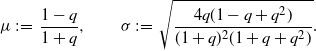 \begin{equation} \mu\;:\!=\;\frac{1-q}{1+q} , \qquad \sigma\;:\!=\;\sqrt{\frac{4q(1-q+q^2)}{(1+q)^2(1+q+q^2)}}.\end{equation}
Then, as
 $n \rightarrow \infty$
,
$n \rightarrow \infty$
,
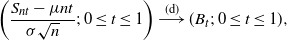 \begin{equation*} \left(\frac{S_{nt} -\mu nt}{\sigma \sqrt{n}}; \, 0 \le t \le 1 \right) \stackrel{(\textrm{d})}{\longrightarrow} ( B_t; \, 0 \le t \le 1 ),\end{equation*}
where
 $\stackrel{(\textrm{d})}{\longrightarrow}$
denotes the weak convergence in C[0,1] equipped with the sup-norm topology.
$\stackrel{(\textrm{d})}{\longrightarrow}$
denotes the weak convergence in C[0,1] equipped with the sup-norm topology.
Given the above theorem, it is natural to consider the dragged-down walk
 $S^{q}_k: = S_k - \mu k$
,
$S^{q}_k: = S_k - \mu k$
,
 $0 \le k \le n$
. Let
$0 \le k \le n$
. Let
 $G^q_n$
,
$G^q_n$
,
 $G^{q,\max}_n$
,
$G^{q,\max}_n$
,
 $\Gamma^q_n$
, and
$\Gamma^q_n$
, and
 $N^q_n$
be the Lévy statistics corresponding to the dragged-down walk. As a direct consequence of Theorem 2.1, the random variables
$N^q_n$
be the Lévy statistics corresponding to the dragged-down walk. As a direct consequence of Theorem 2.1, the random variables
 $G^q_n/n$
,
$G^q_n/n$
,
 $G^{q,\max}_n/n$
,
$G^{q,\max}_n/n$
,
 $\Gamma^q_n/n$
, and
$\Gamma^q_n/n$
, and
 $N^q_n/n$
all converge to the arcsine distribution whose density is given by (1.1).
$N^q_n/n$
all converge to the arcsine distribution whose density is given by (1.1).
The proof of Theorem 2.1 is given in Section 3, and makes use of the Gnedin–Olshanski construction of the Mallows(q) permutation. By letting
 $q= 1$
, we get the scaling limit of a random walk generated from the uniform permutation, which has recently been proved in the framework of zigzag graphs [64, Proposition 9.1]. For this case, we have the following corollary.
$q= 1$
, we get the scaling limit of a random walk generated from the uniform permutation, which has recently been proved in the framework of zigzag graphs [64, Proposition 9.1]. For this case, we have the following corollary.
Corollary 2.2 Let
 $(S_k; \, 0 \le k \le n)$
be a random walk generated from the uniform permutation of
$(S_k; \, 0 \le k \le n)$
be a random walk generated from the uniform permutation of
 $[n+1]$
. Then, as
$[n+1]$
. Then, as
 $n \rightarrow \infty$
,
$n \rightarrow \infty$
,
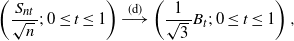 \begin{equation*} \left(\frac{S_{nt}}{\sqrt{n}\,}; \, 0 \le t \le 1 \right) \stackrel{(\textrm{d})}{\longrightarrow} \left(\frac{1}{\sqrt{3}\,}B_t; \, 0 \le t \le 1 \right),\end{equation*}
where
 $\stackrel{(\textrm{d})}{\longrightarrow}$
denotes the weak convergence in C[0,Reference Akahori1] equipped with the sup-norm topology. Consequently, as
$\stackrel{(\textrm{d})}{\longrightarrow}$
denotes the weak convergence in C[0,Reference Akahori1] equipped with the sup-norm topology. Consequently, as
 $n \rightarrow \infty$
, the random variables
$n \rightarrow \infty$
, the random variables
 $G_n/n$
,
$G_n/n$
,
 $G^{\max}_n/n$
, and
$G^{\max}_n/n$
, and
 $\Gamma_n/n$
converge in distribution to the arcsine law given by the density (1.1).
$\Gamma_n/n$
converge in distribution to the arcsine law given by the density (1.1).
Now that the limiting process has been established, we can ask the following question.
Question 2.3. For a random walk generated from the Mallows(q) permutation of
 $[{n+1}]$
, what are the error bounds between
$[{n+1}]$
, what are the error bounds between
 $G^q_n/n$
,
$G^q_n/n$
,
 $G^{q,\max}/n$
,
$G^{q,\max}/n$
,
 $\Gamma^q_n/n$
,
$\Gamma^q_n/n$
,
 $N^q_n/n$
, and their arcsine limit?
$N^q_n/n$
, and their arcsine limit?
While we cannot answer these questions directly, we were able to prove partial and related results. To state these, we need some notation. For two random variables X and Y, we define the Wasserstein distance as
 $d_{\textrm{W}}(X, Y)\;:\!=\;\sup_{h \in \textrm{Lip}(1)} |\mathbb{E}h(X) - \mathbb{E}h(Y)|$
, where
$d_{\textrm{W}}(X, Y)\;:\!=\;\sup_{h \in \textrm{Lip}(1)} |\mathbb{E}h(X) - \mathbb{E}h(Y)|$
, where
 $\textrm{Lip}(1)\;:\!=\;\{h : |h(x) - h(y)| \le |x - y|\}$
is the class of Lipschitz-continuous functions with Lipschitz constant 1. For
$\textrm{Lip}(1)\;:\!=\;\{h : |h(x) - h(y)| \le |x - y|\}$
is the class of Lipschitz-continuous functions with Lipschitz constant 1. For
 $m \ge 1$
, let
$m \ge 1$
, let
 $\textrm{BC}^{m,1}$
be the class of bounded functions that have m bounded and continuous derivatives and whose mth derivative is Lipschitz continuous. Let
$\textrm{BC}^{m,1}$
be the class of bounded functions that have m bounded and continuous derivatives and whose mth derivative is Lipschitz continuous. Let
 $\Vert h\Vert_{\infty}$
be the sup-norm of h, and if the kth derivative of h exists, let
$\Vert h\Vert_{\infty}$
be the sup-norm of h, and if the kth derivative of h exists, let
 \begin{equation*} |h|_k\;:\!=\;\left\| \frac{\textrm{d}^k h}{\textrm{d} x^k} \right\|_{\infty} , \qquad |h|_{k,1}\;:\!=\;\sup_{x,y} \Bigg\lvert \frac{\textrm{d}^k h(x)}{\textrm{d} x^k} - \frac{\textrm{d}^k h(y)}{\textrm{d} y^k} \Bigg\lvert \frac{1}{|x - y|}.\end{equation*}
The following results hold true for a simple random walk. However, we have strong numerical evidence that they are also true for the permutation generated random walk; see Conjecture 2.5.
Theorem 2.4 Let
 $(S_{k}; \, 0 \le k \le 2n)$
be a simple symmetric random walk. Then
$(S_{k}; \, 0 \le k \le 2n)$
be a simple symmetric random walk. Then
 \begin{equation}\mathbb{P}(N_{2n} = 2k) = \alpha_{2k,2n} \qquad \text{for } k \in \{0, \ldots , n\}.\end{equation}
Moreover, let Z be an arcsine distributed random variable; then
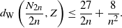 \begin{equation}d_{\textrm{W}}\left(\frac{N_{2n}}{2n},Z\right) \le \frac{27}{2n} + \frac{8}{n^2}.\end{equation}
Furthermore, for any
 $h \in \textrm{BC}^{2,1}$
,
$h \in \textrm{BC}^{2,1}$
,
 \begin{equation}\Bigg\lvert\mathbb{E}h\left(\frac{N_{2n}}{2n}\right) - \mathbb{E}h(Z) \Bigg\lvert \leq \frac{4 |h|_2 + |h|_{2,1}}{64n} + \frac{|h|_{2,1}}{64n^2}.\end{equation}
Identity (2.2) can be found in [Reference Feller28], the bound (2.3) was proved by [Reference Goldstein and Reinert34], and the proof of (2.4) is deferred to Section 4.
Conjecture 2.5 For a uniform random permutation generated random walk of length
 $2n+1$
, the probability that there are 2k edges above the origin equals
$2n+1$
, the probability that there are 2k edges above the origin equals
 $\alpha_{2n,2k}$
, which is the same as that of a simple random walk (see (1.2)).
$\alpha_{2n,2k}$
, which is the same as that of a simple random walk (see (1.2)).
For a walk generated from a permutation of
 $[n+1]$
, call it a positive walk if
$[n+1]$
, call it a positive walk if
 $N_n = n$
, and a negative walk if
$N_n = n$
, and a negative walk if
 $N_n = 0$
. In [Reference Bernardi, Duplantier and Nadeau7] it was proved that the number of positive walks
$N_n = 0$
. In [Reference Bernardi, Duplantier and Nadeau7] it was proved that the number of positive walks
 $b_n$
generated from permutations of [n] is
$b_n$
generated from permutations of [n] is
 $n!!\,(n-2)!!$
if n is odd, and
$n!!\,(n-2)!!$
if n is odd, and
 $[(n-1)!!]^2$
if n is even. Computer enumerations suggest that
$[(n-1)!!]^2$
if n is even. Computer enumerations suggest that
 $c_{2k,2n+1}$
, the number of walks generated from permutations of
$c_{2k,2n+1}$
, the number of walks generated from permutations of
 $[2n+1]$
with 2k edges above the origin, satisfies
$[2n+1]$
with 2k edges above the origin, satisfies
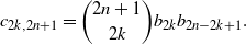 \begin{equation}c_{2k, 2n+1} = \binom{2n+1}{2k} b_{2k} b_{2n-2k+1}.\end{equation}
Note that, for the special cases
 $k = 0$
and
$k = 0$
and
 $k=n$
, the formula (2.5) agrees with the known results in [Reference Bernardi, Duplantier and Nadeau7]. The formula (2.5) suggests a bijection between permutations of
$k=n$
, the formula (2.5) agrees with the known results in [Reference Bernardi, Duplantier and Nadeau7]. The formula (2.5) suggests a bijection between permutations of
 $[2n+1]$
with 2k positive edges and pairs of permutations of disjoint subsets of
$[2n+1]$
with 2k positive edges and pairs of permutations of disjoint subsets of
 $2n + 1$
of respective cardinality 2k and
$2n + 1$
of respective cardinality 2k and
 $2n+1-2k$
whose associated descent walks are positive. A naive idea is to break the walk into positive and negative excursions, and exclude the final visit to the origin before crossing to the other side of the origin in each excursion [Reference Andersen2, Reference Bertoin9]. However, this approach does not work since not all pairs of positive walks are obtainable. For example, for
$2n+1-2k$
whose associated descent walks are positive. A naive idea is to break the walk into positive and negative excursions, and exclude the final visit to the origin before crossing to the other side of the origin in each excursion [Reference Andersen2, Reference Bertoin9]. However, this approach does not work since not all pairs of positive walks are obtainable. For example, for
 $n = 3$
, the pair (1,2,3) and (7,6,5,4) cannot be obtained. If Conjecture 2.5 holds, we get the arcsine law as the limiting distribution of
$n = 3$
, the pair (1,2,3) and (7,6,5,4) cannot be obtained. If Conjecture 2.5 holds, we get the arcsine law as the limiting distribution of
 $N_{2n}/2n$
with error bounds.
$N_{2n}/2n$
with error bounds.
While we are not able to say much about
 $G_n$
,
$G_n$
,
 $G^{\max}_n$
, and
$G^{\max}_n$
, and
 $\Gamma_n$
with respect to a random walk generated from the uniform permutation for finite n, we can prove that the limiting distributions of these Lévy statistics are still arcsine; this is a consequence of the fact that the scaled random walks converge to Brownian motion.
$\Gamma_n$
with respect to a random walk generated from the uniform permutation for finite n, we can prove that the limiting distributions of these Lévy statistics are still arcsine; this is a consequence of the fact that the scaled random walks converge to Brownian motion.
Classical results in [Reference Komlós, Major and Tusnády41, Reference Komlós, Major and Tusnády42, Reference Skorokhod57] provide strong embeddings of a random walk with independent increments into Brownian motion. In view of Theorem 2.1, it is also interesting to understand the strong embedding of a random walk generated from the Mallows(q) permutation. We have the following result.
Theorem 2.6 Fix
 $0< q\leq 1$
, and let
$0< q\leq 1$
, and let
 $(S_k; \, 0 \le k \le n)$
be a random walk generated from the Mallows(q) permutation of
$(S_k; \, 0 \le k \le n)$
be a random walk generated from the Mallows(q) permutation of
 $[n+1]$
. Let
$[n+1]$
. Let
 $\mu$
and
$\mu$
and
 $\sigma$
be defined by (2.1), and let
$\sigma$
be defined by (2.1), and let
 \begin{equation*}\beta\;:\!=\;\frac{2}{\sigma(1+q)} , \qquad \eta\;:\!=\;\frac{2q}{1-q+q^2}.\end{equation*}
Then, there exist universal constants
 $n_0, c_1, c_2 > 0$
such that, for any
$n_0, c_1, c_2 > 0$
such that, for any
 $\varepsilon \in (0,1)$
and
$\varepsilon \in (0,1)$
and
 $n \ge n_0$
, we can construct
$n \ge n_0$
, we can construct
 $(S_t; \, 0 \le t \le n)$
and
$(S_t; \, 0 \le t \le n)$
and
 $(B_t; \, 0 \le t \le n)$
on the same probability space such that
$(B_t; \, 0 \le t \le n)$
on the same probability space such that
 \begin{equation*} \mathbb{P}\left(\sup_{0 \le t \le n} | \frac{1}{\sigma} (S_t - \mu t )- B_t | > c_1 n^{\frac{1 + \varepsilon}{4}} (\log n)^{\frac{1}{2}} \beta \right) \le \frac{c_2(\beta^6 + \eta)}{\beta^2 n^{\varepsilon} \log n}.\end{equation*}
In fact, a much more general result, namely a strong embedding for m-dependent random walks, is proved in Section 5.
Also note that there is substantial literature studying the relations between random permutations and Brownian motion. Classical results were surveyed in [Reference Arratia, Barbour and Tavaré3, Reference Pitman50]; see also [Reference Bassino, Bouvel, Féray, Gerin and Pierrot5, Reference Hoffman, Rizzolo and Slivken35, Reference Hoffman, Rizzolo and Slivken36, Reference Janson38] for recent progress on the Brownian limit of pattern-avoiding permutations.
3. Proof of Theorem 2.1
In this section we prove Theorem 2.1. To establish the result, we first show that the Mallows(q) permutation can be constructed from one-dependent increments
 $(X_1, \ldots,$
 $X_n)$
; that is,
$X_n)$
; that is,
 $(X_1, \ldots,X_j)$
are independent of
$(X_1, \ldots,X_j)$
are independent of
 $(X_{j+2}, \ldots, X_n)$
for each
$(X_{j+2}, \ldots, X_n)$
for each
 $j \in [n-2]$
. Then we calculate its moments and use an invariance principle.
$j \in [n-2]$
. Then we calculate its moments and use an invariance principle.
Gnedin and Olshanski [Reference Gnedin and Olshanski33] provide a nice construction of the Mallows(q) permutation, which is implicit in the original work [Reference Mallows47]. This representation of the Mallows(q) permutation plays an important role in the proof of Theorem 2.1.
For
 $n>0$
and
$n>0$
and
 $0 < q < 1$
, let
$0 < q < 1$
, let
 $\mathcal{G}_{q,n}$
be a truncated geometric random variable on [n] whose probability distribution is given by
$\mathcal{G}_{q,n}$
be a truncated geometric random variable on [n] whose probability distribution is given by
 \begin{equation*}\mathbb{P}(\mathcal{G}_{q,n} = k) = \frac{q^{k-1}(1-q)}{1- q^n} \qquad \text{for } k \in [n].\end{equation*}
Since
 $\mathbb{P}(\mathcal{G}_{q,n} = k)\to n^{-1}$
if
$\mathbb{P}(\mathcal{G}_{q,n} = k)\to n^{-1}$
if
 $q\to1$
, we can extend the definition of
$q\to1$
, we can extend the definition of
 $\mathcal{G}_{q,n}$
to
$\mathcal{G}_{q,n}$
to
 $q=1$
, which is just the uniform distribution on [n]. The Mallows(q) permutation
$q=1$
, which is just the uniform distribution on [n]. The Mallows(q) permutation
 $\pi$
of [n] is constructed as follows. Let
$\pi$
of [n] is constructed as follows. Let
 $(Y_k; \, k \in [n])$
be a sequence of independent random variables, where
$(Y_k; \, k \in [n])$
be a sequence of independent random variables, where
 $Y_k$
is distributed as
$Y_k$
is distributed as
 $\mathcal{G}_{n+1-k}$
. Set
$\mathcal{G}_{n+1-k}$
. Set
 $\pi_1\;:\!=\;Y_1$
and, for
$\pi_1\;:\!=\;Y_1$
and, for
 $k \ge 2$
, let
$k \ge 2$
, let
 $\pi_k\;:\!=\;\psi(Y_k)$
where
$\pi_k\;:\!=\;\psi(Y_k)$
where
 $\psi$
is the increasing bijection from
$\psi$
is the increasing bijection from
 $[n - k +1]$
to
$[n - k +1]$
to
 $[n] \setminus \{ \pi_1, \pi_2, \ldots, \pi_{k-1} \}$
. That is, pick
$[n] \setminus \{ \pi_1, \pi_2, \ldots, \pi_{k-1} \}$
. That is, pick
 $\pi_1$
according to
$\pi_1$
according to
 $\mathcal{G}_{q,n}$
, and remove
$\mathcal{G}_{q,n}$
, and remove
 $\pi_1$
from [n]. Then pick
$\pi_1$
from [n]. Then pick
 $\pi_2$
as the
$\pi_2$
as the
 $\mathcal{G}_{q,n-1}$
th smallest element of
$\mathcal{G}_{q,n-1}$
th smallest element of
 $[n] \setminus \{\pi_1\}$
, and remove
$[n] \setminus \{\pi_1\}$
, and remove
 $\pi_2$
from
$\pi_2$
from
 $[n] \setminus \{\pi_1\}$
; and so on. As an immediate consequence of this construction we have that, for the increments
$[n] \setminus \{\pi_1\}$
; and so on. As an immediate consequence of this construction we have that, for the increments
 $(X_k; \, k \in [n])$
of a random walk generated from the Mallows(q) permutation of
$(X_k; \, k \in [n])$
of a random walk generated from the Mallows(q) permutation of
 $[n+1]$
:
$[n+1]$
:
-
for each k,
$\mathbb{P}(X_k = 1) = \mathbb{P}(\mathcal{G}_{q,n+1 -k} \leq \mathcal{G}_{q,n-k}) = 1/(1+q)$
, which is independent of k and n; thus,
$\mathbb{E}X_k = (1-q)/(1+q)$
and
$\textrm{var}\;X_k = 4q/(1+q)^2$
; -
the sequence of increments
$(X_k; \, k \in [n])$
, though not independent, is two-block factor and hence one-dependent; see [Reference de Valk22] for background.


Such a construction is also used in [Reference Gnedin and Olshanski33] to construct a random permutation of positive integers, called the infinite q-shuffle. The latter is further extended in [Reference Pitman and Tang52] to p-shifted permutations as an instance of regenerative permutations, and used in [Reference Holroyd, Hutchcroft and Levy37] to construction symmetric k-dependent q-coloring of positive integers.
If
 $\pi$
is a uniform permutation of [n], the central limit theorem of the number of descents
$\pi$
is a uniform permutation of [n], the central limit theorem of the number of descents
 $\# \mathcal{D}(\pi)$
is well known:
$\# \mathcal{D}(\pi)$
is well known:
 \begin{equation*} \frac{1}{\sqrt{n}\,}\left(\# \mathcal{D}(\pi) - \frac{n}{2}\right) \stackrel{(\textrm{d})}{\longrightarrow} \frac{1}{\sqrt{12}\,} \mathcal{N}(0,1),\end{equation*}
where
 $\mathcal{N}(0,1)$
is a standard normal distribution. See See [Reference Chatterjee and Diaconis18, Section 3] for a survey of six different approaches to proving this fact. The central limit theorem of the number of descents of the Mallows(q) permutation is known, and is as follows.
$\mathcal{N}(0,1)$
is a standard normal distribution. See See [Reference Chatterjee and Diaconis18, Section 3] for a survey of six different approaches to proving this fact. The central limit theorem of the number of descents of the Mallows(q) permutation is known, and is as follows.
Lemma 3.1.
(Proposition 5.2 of [Reference Borodin, Diaconis and Fulman14].) Fix
 $0< q\leq 1$
, let
$0< q\leq 1$
, let
 $\pi$
be the Mallows(q) permutation of [n], and let
$\pi$
be the Mallows(q) permutation of [n], and let
 $\# \mathcal{D}(\pi)$
be the number of descents of
$\# \mathcal{D}(\pi)$
be the number of descents of
 $\pi$
. Then
$\pi$
. Then
 \begin{equation*}\mathbb{E} \# \mathcal{D}(\pi) = \frac{(n-1)q}{1+q} , \qquad \textrm{var} \# \mathcal{D}(\pi) = q \frac{(1-q+q^2)n -1 + 3q - q^2}{(1+q)^2(1+q+q^2)}.\end{equation*}
Moreover,
 \begin{equation*} \frac{1}{\sqrt{n}\,}\left(\# \mathcal{D}(\pi) - \frac{nq}{1+q}\right) \stackrel{(\textrm{d})}{\longrightarrow} \mathcal{N}\left(0, \frac{q(1-q+q^2)}{(1+q)^2(1+q+q^2)} \right).\end{equation*}
We are now ready to prove Theorem 2.1.
Proof of Theorem 2.1. We first recall [Reference Billingsley11, Theorem 5.1]: Let
 $X_1,X_2,\dots$
be an m-dependent sequence, and let
$X_1,X_2,\dots$
be an m-dependent sequence, and let
 $s_n^2=\sum_{i=1}^n\mathbb{E}X_i^2$
. If
$s_n^2=\sum_{i=1}^n\mathbb{E}X_i^2$
. If
 $\mathbb{E} X_n=0$
for all
$\mathbb{E} X_n=0$
for all
 $n\geq 1$
, if
$n\geq 1$
, if
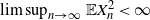 $\lim\sup_{n\to\infty} \mathbb{E} X_n^2<\infty$
, if
$\lim\sup_{n\to\infty} \mathbb{E} X_n^2<\infty$
, if
 $|s_n^2 -n\sigma^2| = \textrm{O}(1)$
for some
$|s_n^2 -n\sigma^2| = \textrm{O}(1)$
for some
 $\sigma^2>0$
, and if
$\sigma^2>0$
, and if
 \begin{equation*}\lim_{n\to\infty} s_n^{-2-\delta}\sum_{i=1}^n\mathbb{E} X_i^{2+\delta}=0\end{equation*}
for some
 $\delta>0$
, then the invariance principle holds for the sequence
$\delta>0$
, then the invariance principle holds for the sequence
 $X_1,X_2,\dots$
with normalizing factor
$X_1,X_2,\dots$
with normalizing factor
 $\sigma n^{1/2}$
; that is, the sequence of processes
$\sigma n^{1/2}$
; that is, the sequence of processes
 $S_n(t)$
,
$S_n(t)$
,
 $0\leq t\leq 1$
, defined by
$0\leq t\leq 1$
, defined by
 $S_n(k/n)=\sigma^{-1} n^{-1/2}\sum_{i=1}^k X_i$
for
$S_n(k/n)=\sigma^{-1} n^{-1/2}\sum_{i=1}^k X_i$
for
 $0\leq k\leq n$
and linearly interpolated otherwise, converges weakly to a standard Brownian motion on the unit interval with respect to the Borel sigma-algebra generated by the topology of the supremum norm on the space of continuous functions on the unit interval.
$0\leq k\leq n$
and linearly interpolated otherwise, converges weakly to a standard Brownian motion on the unit interval with respect to the Borel sigma-algebra generated by the topology of the supremum norm on the space of continuous functions on the unit interval.
Since the increments of a permutation generated random walk are one-dependent, the functional central limit theorem is an immediate consequence of [Reference Billingsley11, Theorem 5.1] and the moments in Lemma 3.1.
4. Proof of Theorem 2.4
4.1. Stein’s method for the arcsine distribution
It is well known that for a simple symmetric walk,
 $G_{2n}$
and
$G_{2n}$
and
 $N_{2n}$
are discrete arcsine distributed, thus converging to the arcsine distribution. To apply Stein’s method for arcsine approximation we first need a characterizing operator.
$N_{2n}$
are discrete arcsine distributed, thus converging to the arcsine distribution. To apply Stein’s method for arcsine approximation we first need a characterizing operator.
Lemma 4.1 A random variable Z is arcsine distributed if and only if
 \begin{equation*}\mathbb{E} [ Z(1-Z) f'(Z) + ( 1/2 - Z) f(Z) ] = 0\end{equation*}
for all functions
 $f \in \textrm{BC}^{2,1}[0,1]$
.
$f \in \textrm{BC}^{2,1}[0,1]$
.
To apply Stein’s method, we proceed as follows. Let Z be an arcsine distributed random variable. Then, for any
 $h\in \text{Lip}(1)$
or
$h\in \text{Lip}(1)$
or
 $h \in \textrm{BC}^{2,1}[0,1]$
, assume we have a function f that solves
$h \in \textrm{BC}^{2,1}[0,1]$
, assume we have a function f that solves
 \begin{align}x(1-x) f'(x) + ( 1/2- x ) f(x) = h(x) - \mathbb{E} h(Z).\end{align}
For an arbitrary random variable W, replace x with W in (4.1) and, by taking expectations, this yields an expression for
 $\mathbb E h(W)-\mathbb E h(Z)$
in terms of just W and f. Our goal is therefore to bound the expectation of the left-hand side of (4.1) by utilizing properties of f. Extending [Reference Döbler24, Reference Goldstein and Reinert34] developed Stein’s method for the beta distribution (of which arcsine is a special case) and gave an explicit Wasserstein bound between the discrete and the continuous arcsine distributions. We will use the framework from [Reference Gan, Röllin and Ross29] to calculate error bounds for the class of test functions
$\mathbb E h(W)-\mathbb E h(Z)$
in terms of just W and f. Our goal is therefore to bound the expectation of the left-hand side of (4.1) by utilizing properties of f. Extending [Reference Döbler24, Reference Goldstein and Reinert34] developed Stein’s method for the beta distribution (of which arcsine is a special case) and gave an explicit Wasserstein bound between the discrete and the continuous arcsine distributions. We will use the framework from [Reference Gan, Röllin and Ross29] to calculate error bounds for the class of test functions
 $\textrm{BC}^{2,1}$
.
$\textrm{BC}^{2,1}$
.
4.2. Proof of Theorem 2.4
To simplify the notation, let
 $W_n\;:\!=\;N_{2n}/2n$
be the fraction of positive edges of a simple symmetric random walk. Let
$W_n\;:\!=\;N_{2n}/2n$
be the fraction of positive edges of a simple symmetric random walk. Let
 $\Delta_yf(x)\;:\!=\;f(x+y) - f(x)$
. We will use the following known facts for the discrete arcsine distribution. For any function
$\Delta_yf(x)\;:\!=\;f(x+y) - f(x)$
. We will use the following known facts for the discrete arcsine distribution. For any function
 $f \in \textrm{BC}^{m,1}[0,1]$
,
$f \in \textrm{BC}^{m,1}[0,1]$
,
 \begin{equation}\mathbb{E} [ nW_n \left(1 - W_n + \frac{1}{2n} \right) \Delta_{1/n}f \left(W_n - \frac{1}{n} \right) + \left(\frac{1}{2} - W_n \right) f(W_n) ] = 0.\end{equation}
Moreover,
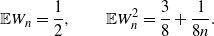 \begin{equation}\mathbb{E}W_n = \frac{1}{2} , \qquad \mathbb{E}W_n^2 = \frac{3}{8} + \frac{1}{8n}.\end{equation}
The identity (4.2) can be read from [Reference Döbler24, Lemma 2.9] and [Reference Goldstein and Reinert34, Proof of Theorem 1.1]. The moments are easily derived by plugging in
 $f(x) = 1$
and
$f(x) = 1$
and
 $f(x) = x$
.
$f(x) = x$
.
Proof of Theorem 2.4. The distribution (2.2) of
 $N_{2n}$
can be found in [Reference Feller28]. The bound (2.3) follows from the fact that
$N_{2n}$
can be found in [Reference Feller28]. The bound (2.3) follows from the fact that
 $N_{2n}$
is discrete arcsine distributed, together with [Reference Goldstein and Reinert34, Theorem 1.2].
$N_{2n}$
is discrete arcsine distributed, together with [Reference Goldstein and Reinert34, Theorem 1.2].
We prove the bound (2.4) using the generator method. Assume
 $h\in\textrm{BC}^{2,1}([0,1])$
, and recall the Stein equation (4.1) for the arcsine distribution. It follows from [Reference Gan, Röllin and Ross29, Theorem 5] that there exists
$h\in\textrm{BC}^{2,1}([0,1])$
, and recall the Stein equation (4.1) for the arcsine distribution. It follows from [Reference Gan, Röllin and Ross29, Theorem 5] that there exists
 $g\in\textrm{BC}^{2,1}([0,1])$
such that
$g\in\textrm{BC}^{2,1}([0,1])$
such that
 $x(1-x) g''(x) + ( 1/2- x ) g'(x) = h(x) - \mathbb{E} h(Z)$
, which is just (4.1) with
$x(1-x) g''(x) + ( 1/2- x ) g'(x) = h(x) - \mathbb{E} h(Z)$
, which is just (4.1) with
 $f = g'$
. We are therefore required to bound the absolute value of
$f = g'$
. We are therefore required to bound the absolute value of
 \begin{equation*} \mathbb{E}h(W_n) - \mathbb{E}h(Z)= \mathbb{E}[W_n(1- W_n) g''(W_n) - \left(\frac{1}{2} - W_n \right) g'(W_n)].\end{equation*}
Applying (4.2) with f being replaced by g’, we obtain
 \begin{equation*}\begin{split}&\mathbb{E}h(W_n) - \mathbb{E}h(Z) \\&\qquad= \mathbb{E} \left[ W_n(1-W_n) g''(W_n) - n W_n \left(1-W_n + \frac{1}{2n}\right) \Delta_{1/n} g'\left(W_n - \frac{1}{n} \right)\right] \\&\qquad= \mathbb{E}\left[W_n(1-W_n) \left(g''(W_n) - n \Delta_{1/n}g' \left(W_n - \frac{1}{n} \right) \right) - \frac{W_n}{2} \Delta_{1/n} g'\left(W_n - \frac{1}{n} \right)\right].\end{split}\end{equation*}
The second term in the expectation is bounded as
 \begin{equation}\Bigg\lvert \mathbb{E} \left[\frac{W_n}{2} \Delta_{1/n} g'\left(W_n - \frac{1}{n} \right) \right] \Bigg\lvert \le \frac{\mathbb{E}W_n}{2} \cdot \frac{|g|_2}{n} = \frac{|g|_2}{4n},\end{equation}
and the first term can be bounded as
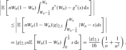 \begin{align}& \Bigg\lvert \mathbb{E} \left[ nW_n(1-W_n) \int_{W_n - \frac{1}{n}}^{W_n} g''(W_n) - g''(x) \, \textrm{d} x \right] \Bigg\lvert \notag \\& \qquad \le \Bigg\lvert \mathbb{E} \left[ nW_n(1-W_n) |g|_{2,1}\int_{W_n - \frac{1}{n}}^{W_n} |W_n -x | dx \right] \Bigg\lvert \notag\\& \qquad = |g|_{2,1} n \mathbb E \left[W_n(1-W_n) \int_0^{\frac1n} s \, \textrm{d} s\right]= \frac{|g|_{2,1}}{16}\left(\frac{1}{n} + \frac{1}{n^2} \right),\end{align}
where the last equality follows from (4.3). Combining (4.4), (4.5), and [Reference Gan, Röllin and Ross29, Theorem 5] (for relating the bounds on derivatives g with derivatives of h) yields the desired bound.
Remark 4.2 The above bound is essentially sharp. Take
 $h(x) =\frac{x^2}{2}$
,
$h(x) =\frac{x^2}{2}$
,
 $\mathbb E h(W_n) - \mathbb E h(Z) = -\frac{1}{16n}$
, and the above bound gives
$\mathbb E h(W_n) - \mathbb E h(Z) = -\frac{1}{16n}$
, and the above bound gives
 $| \mathbb E h(W_n) - \mathbb E h(Z)| \leq \frac{1}{16n} + \frac{1}{64n^2}$
.
$| \mathbb E h(W_n) - \mathbb E h(Z)| \leq \frac{1}{16n} + \frac{1}{64n^2}$
.
5. Proof of Theorem 2.6
In this section we prove Theorem 2.6. To this end, we prove a general result for strong embeddings of a random walk with finitely dependent increments.
5.1. Strong embeddings of m-dependent walks
Let n, m be positive integers. Let
 $(X_i; \, i\in [n])$
be a sequence of m-dependent random variables. That is,
$(X_i; \, i\in [n])$
be a sequence of m-dependent random variables. That is,
 $\{X_1, \ldots, X_j\}$
is independent of
$\{X_1, \ldots, X_j\}$
is independent of
 $\{X_{j+m+1}, \ldots, X_n\}$
for each
$\{X_{j+m+1}, \ldots, X_n\}$
for each
 $j \in [n-m-1]$
. Let
$j \in [n-m-1]$
. Let
 $(S_k; \, k\in \{0,1,\dots, n\})$
be a random walk with increments
$(S_k; \, k\in \{0,1,\dots, n\})$
be a random walk with increments
 $X_i$
, and
$X_i$
, and
 $(S_t; \, 0 \le t \le n)$
be the linear interpolation of
$(S_t; \, 0 \le t \le n)$
be the linear interpolation of
 $(S_k; \, k\in \{0,1,\dots, n\})$
. Assume that the random variables
$(S_k; \, k\in \{0,1,\dots, n\})$
. Assume that the random variables
 $X_i$
are centered and scaled such that
$X_i$
are centered and scaled such that
 $\mathbb{E}X_i = 0$
for all
$\mathbb{E}X_i = 0$
for all
 $i \in [n]$
and
$i \in [n]$
and
 $\textrm{var}(S_n) = n$
. Let
$\textrm{var}(S_n) = n$
. Let
 $(B_t; \, t \ge 0)$
be a one-dimensional standard Brownian motion. The idea of strong embedding is to couple
$(B_t; \, t \ge 0)$
be a one-dimensional standard Brownian motion. The idea of strong embedding is to couple
 $(S_t; \, 0 \le t \le n)$
and
$(S_t; \, 0 \le t \le n)$
and
 $(B_t; \, 0 \le t \le n)$
in such a way that
$(B_t; \, 0 \le t \le n)$
in such a way that
 \begin{equation}\mathbb{P}\left(\sup_{0 \le t \le n}|S_t - B_t| > b_n \right) = p_n \end{equation}
for some
 $b_n = o(n^{\frac{1}{2}})$
and
$b_n = o(n^{\frac{1}{2}})$
and
 $p_n = o(1)$
as
$p_n = o(1)$
as
 $n \rightarrow \infty$
(note that the typical fluctuation of
$n \rightarrow \infty$
(note that the typical fluctuation of
 $B_n$
is
$B_n$
is
 $O(n^{\frac{1}{2}}$
)).
$O(n^{\frac{1}{2}}$
)).
The study of such embeddings dates back to [Reference Skorokhod57]. When the Xs are independent and identically distributed, [Reference Strassen61] obtained (5.1) with
 $b_n = \mathcal{O}(n^{\frac{1}{4}} (\log n)^{\frac{1}{2}} (\log \log n)^{\frac{1}{4}})$
; [Reference Csörgö and Révész20] used a novel approach to prove that under the additional conditions
$b_n = \mathcal{O}(n^{\frac{1}{4}} (\log n)^{\frac{1}{2}} (\log \log n)^{\frac{1}{4}})$
; [Reference Csörgö and Révész20] used a novel approach to prove that under the additional conditions
 $\mathbb{E}X_i^3 =0$
and
$\mathbb{E}X_i^3 =0$
and
 $\mathbb{E}X_i^8 < \infty$
we get
$\mathbb{E}X_i^8 < \infty$
we get
 $b_n = \mathcal{O}(n^{\frac{1}{6} + \varepsilon})$
for any
$b_n = \mathcal{O}(n^{\frac{1}{6} + \varepsilon})$
for any
 $\varepsilon > 0$
; and [Reference Komlós, Major and Tusnády41, Reference Komlós, Major and Tusnády42] further obtained
$\varepsilon > 0$
; and [Reference Komlós, Major and Tusnády41, Reference Komlós, Major and Tusnády42] further obtained
 $b_n = \mathcal{O}(\log n)$
under a finite moment-generating function assumption. See also [Reference Bhattacharjee and Goldstein10, Reference Chatterjee17] for recent developments.
$b_n = \mathcal{O}(\log n)$
under a finite moment-generating function assumption. See also [Reference Bhattacharjee and Goldstein10, Reference Chatterjee17] for recent developments.
We use the argument from [Reference Csörgö and Révész20] to obtain the following result for m-dependent random variables.
Theorem 5.1 Let
 $(S_t; \, 0 \le t \le n)$
be the linear interpolation of partial sums of m-dependent random variables
$(S_t; \, 0 \le t \le n)$
be the linear interpolation of partial sums of m-dependent random variables
 $(X_i; i\in [n])$
. Assume that
$(X_i; i\in [n])$
. Assume that
 $1 \le m \le n^{\frac{1}{5}}$
and
$1 \le m \le n^{\frac{1}{5}}$
and
 $\mathbb{E}X_i = 0$
for each
$\mathbb{E}X_i = 0$
for each
 $i \in [n]$
. Further assume that
$i \in [n]$
. Further assume that
 $|X_i| \le \beta$
for each
$|X_i| \le \beta$
for each
 $i \in [n]$
, where
$i \in [n]$
, where
 $\beta > 0$
is a constant. Let
$\beta > 0$
is a constant. Let
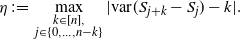 \begin{equation}\eta\;:\!=\;\max_{\substack{k \in [n],\\ j \in \{0,\ldots,n-k\}}} |\textrm{var}(S_{j+k} - S_j) - k|.\end{equation}
For any
 $\varepsilon \in (0,1)$
, if
$\varepsilon \in (0,1)$
, if
 $\eta \le n^{\varepsilon}$
then there exist positive constants
$\eta \le n^{\varepsilon}$
then there exist positive constants
 $n_0$
,
$n_0$
,
 $c_1$
, and
$c_1$
, and
 $c_2$
depending only on
$c_2$
depending only on
 $\varepsilon$
such that, for any
$\varepsilon$
such that, for any
 $n \ge n_0$
, we can define
$n \ge n_0$
, we can define
 $(S_t; \, 0 \le t \le n)$
and
$(S_t; \, 0 \le t \le n)$
and
 $(B_t; \, 0 \le t \le n)$
on the same probability space such that
$(B_t; \, 0 \le t \le n)$
on the same probability space such that
 \begin{equation*}\mathbb{P}\left(\sup_{0 \le t \le n}|S_t - B_t| > c_1 n^{\frac{1 + \varepsilon}{4}} (\log n)^{\frac{1}{2}} m^{\frac{1}{2}} \beta \right) \le \frac{c_2 (m^4\beta^6 + \eta)}{m \beta^2 n^{\varepsilon} \log n}.\end{equation*}
If m and
 $\beta$
are absolute constants and
$\beta$
are absolute constants and
 $\textrm{var}(S_{j+k} - S_j)$
matches k up to an absolute constant, from Theorem 5.1 we get (5.1) with
$\textrm{var}(S_{j+k} - S_j)$
matches k up to an absolute constant, from Theorem 5.1 we get (5.1) with
 $b_n = \mathcal{O}(n^{\frac{1 + \varepsilon}{4}} (\log n)^{\frac{1}{2}})$
and
$b_n = \mathcal{O}(n^{\frac{1 + \varepsilon}{4}} (\log n)^{\frac{1}{2}})$
and
 $p_n = \mathcal{O}(1/(n^{\varepsilon} \log n))$
for any fixed
$p_n = \mathcal{O}(1/(n^{\varepsilon} \log n))$
for any fixed
 $\varepsilon \in (0,1)$
.
$\varepsilon \in (0,1)$
.
Proof of Theorem 2.6. We apply Theorem 5.1 with
 $m = 1$
, and a suitable choice of
$m = 1$
, and a suitable choice of
 $\beta$
and
$\beta$
and
 $\eta$
. By centering and scaling, we consider the walk
$\eta$
. By centering and scaling, we consider the walk
 $(S_t^{'}; \, 0 \le t \le n)$
with increments
$(S_t^{'}; \, 0 \le t \le n)$
with increments
 $X_i^{'} = \frac{1}{\sigma} (X_i -\mu)$
. It is easy to see that
$X_i^{'} = \frac{1}{\sigma} (X_i -\mu)$
. It is easy to see that
 $|X_i^{'}| \le \frac{1}{\sigma} \max( 1- \mu, 1 + \mu ) = \beta$
. According to the result in Section 3,
$|X_i^{'}| \le \frac{1}{\sigma} \max( 1- \mu, 1 + \mu ) = \beta$
. According to the result in Section 3,
 \begin{align*} \mathbb{P}(X_k = X_{k+1} = 1) = \mathbb{P}(\mathcal{G}_{q, n+1-k} \le \mathcal{G}_{q,n-k} \le \mathcal{G}_{q,n-k-1}) & = \frac{1}{(1+q)(1+q+q^2)}, \\ \mathbb{P}(X_k = -1, X_{k+1} = 1) = \mathbb{P}(X_{k+1} = 1) - \mathbb{P}(X_k = X_{k+1} = 1) & = \frac{q}{1 + q + q^2}, \\ \mathbb{P}(X_k = X_{k+1} = -1) = \mathbb{P}(X_{k} = -1) - \mathbb{P}(X_k = -1, X_{k+1} = 1) & = \frac{q^3}{(1+q)(1+q+q^2)}.\end{align*}
By the one-dependence property, elementary computation shows that, for
 $k \le n$
,
$k \le n$
,
 $\textrm{var} S_k^{'} = k + \eta$
, which leads to the desired result.
$\textrm{var} S_k^{'} = k + \eta$
, which leads to the desired result.
5.2. Proof of Theorem 5.1
The proof of Theorem 5.1 boils down to a series of lemmas. In the following, ‘sufficiently large n’ means
 $n\geq n_0$
for some
$n\geq n_0$
for some
 $n_0$
depending only on
$n_0$
depending only on
 $\varepsilon$
. We use C and c to denote positive constants depending only on
$\varepsilon$
. We use C and c to denote positive constants depending only on
 $\varepsilon$
and may differ in different expressions. Let
$\varepsilon$
and may differ in different expressions. Let
 $d\;:\!=\;\lceil n^{\frac{1-\varepsilon}{2}} \rceil$
, where
$d\;:\!=\;\lceil n^{\frac{1-\varepsilon}{2}} \rceil$
, where
 $\lceil x \rceil$
is the least integer greater than or equal to x. We divide the interval [0,n] into d subintervals by points
$\lceil x \rceil$
is the least integer greater than or equal to x. We divide the interval [0,n] into d subintervals by points
 $\lceil jn/d \rceil$
,
$\lceil jn/d \rceil$
,
 $j\in [d]$
, each with length
$j\in [d]$
, each with length
 $l=\lceil n/d \rceil$
or
$l=\lceil n/d \rceil$
or
 $l=\lceil n/d \rceil-1$
. The following results hold for both values of l.
$l=\lceil n/d \rceil-1$
. The following results hold for both values of l.
Lemma 5.2 Under the assumptions in Theorem 5.1, we have, for sufficiently large n,
 \begin{equation}4m\beta^2\geq 1 , \qquad l\geq 6m\log n .\end{equation}
Proof. By the definition of
 $\eta$
in (5.2), the m-dependence assumption, and the upper bounds on
$\eta$
in (5.2), the m-dependence assumption, and the upper bounds on
 $\eta$
and
$\eta$
and
 $|X_i|$
, we have
$|X_i|$
, we have
 \begin{equation*}n-n^\varepsilon \leq n-\eta \leq \textrm{var} S_n = \sum_{i = 1}^n \sum_{j: |j - i| \le m} \mathbb{E}X_i X_j \le n(2m+1)\beta^2 , \qquad m \ge 1,\end{equation*}
which implies
 $4m \beta^2 \ge 1$
for sufficiently large n. The second bound in (5.3) follows from the fact that
$4m \beta^2 \ge 1$
for sufficiently large n. The second bound in (5.3) follows from the fact that
 $m \le n^{\frac{1}{5}}$
and
$m \le n^{\frac{1}{5}}$
and
 $l \sim n^{\frac{1 + \varepsilon}{2}}$
.
$l \sim n^{\frac{1 + \varepsilon}{2}}$
.
Given two probability measures
 $\mu$
and
$\mu$
and
 $\nu$
on
$\nu$
on
 $\mathbb{R}$
, define their Wasserstein-2 distance by
$\mathbb{R}$
, define their Wasserstein-2 distance by
 \begin{equation*} d_{W_2}(\mu, \nu) = \left( \inf_{\pi \in \Gamma(\mu, \nu)} \int |x-y|^2 \, \textrm{d} \pi(x,y)\right)^{\frac{1}{2}},\end{equation*}
where
 $\Gamma(\mu, \nu)$
is the space of all probability measures on
$\Gamma(\mu, \nu)$
is the space of all probability measures on
 $\mathbb{R}^2$
with
$\mathbb{R}^2$
with
 $\mu$
and
$\mu$
and
 $\nu$
as marginals. We will use the following Wasserstein-2 bound from [Reference Fang27]. We use
$\nu$
as marginals. We will use the following Wasserstein-2 bound from [Reference Fang27]. We use
 $\mathcal{N}(\mu,\sigma^2)$
to denote the normal distribution with mean
$\mathcal{N}(\mu,\sigma^2)$
to denote the normal distribution with mean
 $\mu$
and variance
$\mu$
and variance
 $\sigma^2$
.
$\sigma^2$
.
Lemma 5.3. (Corollary 2.3 of [Reference Fang27].) Let
 $W=\sum_{i=1}^n \xi_i$
be a sum of m-dependent random variables with
$W=\sum_{i=1}^n \xi_i$
be a sum of m-dependent random variables with
 $\mathbb{E} \xi_i=0$
and
$\mathbb{E} \xi_i=0$
and
 $\mathbb{E} W^2=1$
. We have
$\mathbb{E} W^2=1$
. We have
 \begin{equation}d_{W_2}(\mathcal{L}(W), \mathcal{N}(0,1))\leq C_0\left\{m^2 \sum_{i=1}^n \mathbb{E}|\xi_i|^3+m^{3/2} \left(\sum_{i=1}^n \mathbb{E} \xi_i^4\right)^{1/2} \right\},\end{equation}
where
 $C_0$
is an absolute constant.
$C_0$
is an absolute constant.
Specializing the above lemma to bounded random variables, we obtain the following result.
Lemma 5.4 Under the assumptions in Theorem 5.1, we have, for sufficiently large n,
 \begin{equation}d_{W_2}(\mathcal{L}(S_{l -m}), \, \mathcal{N}(0,\sigma^2)) \le C m^2 \beta^3,\end{equation}
where
 $\sigma^2\;:\!=\;\textrm{var} S_{l - m}$
.
$\sigma^2\;:\!=\;\textrm{var} S_{l - m}$
.
Proof. Applying (5.4) to
 $\sigma^{-1} S_{l-m}$
and using
$\sigma^{-1} S_{l-m}$
and using
 $|X_i|\leq \beta$
, we obtain
$|X_i|\leq \beta$
, we obtain
 \begin{align*}d_{W_2}(\mathcal{L}(S_{l-m}), \, \mathcal{N}(0,\sigma^2)) & = \sigma \, d_{W_2}(\sigma^{-1} S_{l-m}, \mathcal{N}(0,1)) \\& \le \sigma C_0\left( lm^2 \left(\frac{\beta}{\sigma} \right)^3 + \left(lm^3 \left(\frac{\beta}{\sigma} \right)^4 \right)^{\frac{1}{2}} \right) \le Cm^2 \beta^3,\end{align*}
where we used
 $4 m \beta^2 \ge 1$
from (5.3), and
$4 m \beta^2 \ge 1$
from (5.3), and
 $\sigma^2 \ge l-m-\eta \ge cl$
for sufficiently large n from (5.2),
$\sigma^2 \ge l-m-\eta \ge cl$
for sufficiently large n from (5.2),
 $m \le n^{\frac{1}{5}}$
,
$m \le n^{\frac{1}{5}}$
,
 $\eta \le n^{\varepsilon}$
,
$\eta \le n^{\varepsilon}$
,
 $l \sim n^{\frac{1 + \varepsilon}{2}}$
, and
$l \sim n^{\frac{1 + \varepsilon}{2}}$
, and
 $\varepsilon \in (0,1)$
.
$\varepsilon \in (0,1)$
.
Lemma 5.5 For sufficiently large n, there exists a coupling of
 $(S_t; \, 0 \le t \le n)$
and
$(S_t; \, 0 \le t \le n)$
and
 $(B_t; \, 0 \le t \le n)$
such that, with
$(B_t; \, 0 \le t \le n)$
such that, with
 $e_j\;:\!=\;(S_{\lceil jn/d \rceil}-S_{\lceil (j-1)n/d \rceil})-(B_{\lceil jn/d \rceil}-B_{\lceil (j-1)n/d \rceil})$
, the sequence
$e_j\;:\!=\;(S_{\lceil jn/d \rceil}-S_{\lceil (j-1)n/d \rceil})-(B_{\lceil jn/d \rceil}-B_{\lceil (j-1)n/d \rceil})$
, the sequence
 $(e_1, \ldots, e_d)$
is one-dependent, and
$(e_1, \ldots, e_d)$
is one-dependent, and
 $\mathbb{E}e_j^2 \le C(m^4 \beta^6 + \eta)$
for all
$\mathbb{E}e_j^2 \le C(m^4 \beta^6 + \eta)$
for all
 $j \in [n]$
.
$j \in [n]$
.
Proof. We use
 $4 m \beta^2 \ge 1$
implicitly below to absorb a few terms into
$4 m \beta^2 \ge 1$
implicitly below to absorb a few terms into
 $Cm^4 \beta^{6}$
. With
$Cm^4 \beta^{6}$
. With
 $\sigma^2$
defined in Lemma 5.4, we have
$\sigma^2$
defined in Lemma 5.4, we have
 $d_{W_2}(\mathcal{N}(0,\sigma^2), \, \mathcal{N}(0,l)) \le \sqrt{|l- \sigma^2|} \le \sqrt{m + \eta}$
. Combining (5.5), the above bound, and the m-dependence assumption, we can couple
$d_{W_2}(\mathcal{N}(0,\sigma^2), \, \mathcal{N}(0,l)) \le \sqrt{|l- \sigma^2|} \le \sqrt{m + \eta}$
. Combining (5.5), the above bound, and the m-dependence assumption, we can couple
 $S_{\lceil jn/d \rceil-m}-S_{\lceil (j-1)n/d \rceil}$
and
$S_{\lceil jn/d \rceil-m}-S_{\lceil (j-1)n/d \rceil}$
and
 $B_{\lceil jn/d \rceil}-B_{\lceil (j-1)n/d \rceil}$
for each
$B_{\lceil jn/d \rceil}-B_{\lceil (j-1)n/d \rceil}$
for each
 $j\in [d]$
independently with
$j\in [d]$
independently with
 $\mathbb{E}[(S_{\lceil jn/d \rceil-m}-S_{\lceil (j-1)n/d \rceil})-(B_{\lceil jn/d \rceil}-B_{\lceil (j-1)n/d \rceil})]^2\leq C( m^4 \beta^6 + \eta)$
. By the m-dependence assumption, we can generate
$\mathbb{E}[(S_{\lceil jn/d \rceil-m}-S_{\lceil (j-1)n/d \rceil})-(B_{\lceil jn/d \rceil}-B_{\lceil (j-1)n/d \rceil})]^2\leq C( m^4 \beta^6 + \eta)$
. By the m-dependence assumption, we can generate
 $X_1,\dots, X_n$
from their conditional distribution given
$X_1,\dots, X_n$
from their conditional distribution given
 $(S_{\lceil jn/d \rceil-m}-S_{\lceil (j-1)n/d \rceil}; \, j\in [d])$
, thus obtaining
$(S_{\lceil jn/d \rceil-m}-S_{\lceil (j-1)n/d \rceil}; \, j\in [d])$
, thus obtaining
 $(S_{t}; \, 0 \le t \le n)$
, and generate
$(S_{t}; \, 0 \le t \le n)$
, and generate
 $(B_t; 0 \le t \le n)$
given
$(B_t; 0 \le t \le n)$
given
 $(B_{\lceil jn/d \rceil}; \, j\in [d])$
. Since
$(B_{\lceil jn/d \rceil}; \, j\in [d])$
. Since
 $\mathbb{E}(S_{\lceil jn/d \rceil}-S_{\lceil jn/d \rceil-m})^2\leq Cm^2\beta^2$
, we have
$\mathbb{E}(S_{\lceil jn/d \rceil}-S_{\lceil jn/d \rceil-m})^2\leq Cm^2\beta^2$
, we have
 $\mathbb{E}(e_j^2)\leq C(m^4\beta^6+\eta)$
. Finally, the one-dependence of
$\mathbb{E}(e_j^2)\leq C(m^4\beta^6+\eta)$
. Finally, the one-dependence of
 $(e_1, \ldots, e_d)$
follows from the m-dependence assumption.
$(e_1, \ldots, e_d)$
follows from the m-dependence assumption.
Lemma 5.6 Let
 $T_j=\sum_{i=1}^j e_i$
,
$T_j=\sum_{i=1}^j e_i$
,
 $j\in [d]$
. For any
$j\in [d]$
. For any
 $b>0$
and sufficiently large n,
$b>0$
and sufficiently large n,
 $\mathbb{P}(\max_{j\in [d]}|T_j|>b )\leq C(m^4\beta^6+\eta ) d/b^2$
.
$\mathbb{P}(\max_{j\in [d]}|T_j|>b )\leq C(m^4\beta^6+\eta ) d/b^2$
.
Proof. Define
 $T_j^{(1)}=\sum_{\substack{i=1,3,5,\dots\\ i\leq j}} e_i$
and
$T_j^{(1)}=\sum_{\substack{i=1,3,5,\dots\\ i\leq j}} e_i$
and
 $T_j^{(2)}=\sum_{\substack{i=2,4,6,\dots\\ i\leq j}} e_i$
. By Lemma 5.5,
$T_j^{(2)}=\sum_{\substack{i=2,4,6,\dots\\ i\leq j}} e_i$
. By Lemma 5.5,
 $T_j^{(1)}$
is a sum of independent random variables with zero mean and finite second moments. By Kolmogorov’s maximal inequality,
$T_j^{(1)}$
is a sum of independent random variables with zero mean and finite second moments. By Kolmogorov’s maximal inequality,
 \begin{equation*}\mathbb{P}\left(\max_{1\leq j\leq d}\big|T_j^{(1)}\big|>\frac{b}{2} \right) \leq \frac{C(m^4 \beta^6+\eta)d}{b^2}.\end{equation*}
The same bound holds for
 $T_j^{(2)}$
. The lemma is proved by the union bound
$T_j^{(2)}$
. The lemma is proved by the union bound
 \begin{equation}\mathbb{P}\left(\max_{j\in [d]}|T_j|>b\right)\leq \mathbb{P}\left(\max_{1\leq j\leq d}|T_j^{(1)}|>\frac{b}{2}\right)+\mathbb{P}\left(\max_{1\leq j\leq d}|T_j^{(2)}|>\frac{b}{2}\right). \end{equation}
Lemma 5.7 For any
 $0<b\leq 4l \beta$
, we have
$0<b\leq 4l \beta$
, we have
 \begin{equation*}\mathbb{P}\left(\max_{j\in [l]} |S_j- j S_l/l|>b\right)\leq 2l \exp\left(-\frac{b^2}{48 l m \beta^2}\right).\end{equation*}
Proof. We first prove a concentration inequality for
 $S_j$
,
$S_j$
,
 $j \in [l]$
, then use the union bound. Let
$j \in [l]$
, then use the union bound. Let
 $h(\theta)=\mathbb{E} \textrm{e}^{\theta S_j}$
, with
$h(\theta)=\mathbb{E} \textrm{e}^{\theta S_j}$
, with
 $h(0)=1$
. Let
$h(0)=1$
. Let
 $S_j^{(i)}=S_j-\sum_{k\in [j]: |k-i|\leq m} X_k$
. Using
$S_j^{(i)}=S_j-\sum_{k\in [j]: |k-i|\leq m} X_k$
. Using
 $\mathbb{E} X_i=0$
,
$\mathbb{E} X_i=0$
,
 $|X_i|\leq \beta$
, the m-dependence assumption, and the inequality (cf. [Reference Chatterjee16, Eq. (7)])
$|X_i|\leq \beta$
, the m-dependence assumption, and the inequality (cf. [Reference Chatterjee16, Eq. (7)])
 \begin{equation*} \Bigg\lvert \frac{\textrm{e}^x-\textrm{e}^y}{x-y} \Bigg\lvert\leq \frac{1}{2}(\textrm{e}^x+\textrm{e}^y),\end{equation*}
we have, for
 $\theta > 0$
and
$\theta > 0$
and
 $\theta (2m+1)\beta\leq 1$
,
$\theta (2m+1)\beta\leq 1$
,
 \begin{equation*}\begin{split}h'(\theta) & =\mathbb{E} (S_j \textrm{e}^{\theta S_j}) =\sum_{i=1}^j \mathbb{E} X_i (\textrm{e}^{\theta S_j}-\textrm{e}^{\theta S_j^{(i)}}) \leq \frac{\theta}{2} \sum_{i=1}^j \mathbb{E} |X_i| \big|S_j-S_j^{(i)}\big| \left(\textrm{e}^{\theta S_j}+\textrm{e}^{\theta S_j^{(i)}} \right)\\&\leq \left(m+\frac{1}{2}\right) \theta l \beta^2 \mathbb{E} \textrm{e}^{\theta S_j} (1+\textrm{e}^{\theta (2m+1)\beta})\leq 6 \theta l m \beta^2 h(\theta).\end{split}\end{equation*}
This implies that
 $\log h(\theta)\leq 3l m \beta^2 \theta^2$
, and
$\log h(\theta)\leq 3l m \beta^2 \theta^2$
, and
 \begin{equation*}\mathbb{P}(S_j>b/2)\leq \textrm{e}^{-\theta b/2} \mathbb{E} \textrm{e}^{\theta S_j}\leq \exp\left(-\frac{b^2}{48 l m \beta^2}\right)\end{equation*}
by choosing
 $\theta=b/(12lm\beta^2)$
, provided that
$\theta=b/(12lm\beta^2)$
, provided that
 $b\leq 4l\beta$
. The same bound holds for
$b\leq 4l\beta$
. The same bound holds for
 $-S_j$
. Consequently,
$-S_j$
. Consequently,
 \begin{align}\mathbb{P}\left(\max_{j\in [l]} |S_j- j S_l/l|>b \right) & \leq \mathbb{P}\left(\max_{j\in [l-1]} |S_j|>b/2\right)+\mathbb{P}\left(|S_l|> b/2\right) \nonumber\\& \leq 2l \exp\left(-\frac{b^2}{48 l m \beta^2}\right). \end{align}
Lemma 5.8 For any
 $b>0$
, we have
$b>0$
, we have
 $\mathbb{P}(\sup_{0\leq t\leq l} |B_t-t B_l/l|>b)\leq 2 \textrm{e}^{-\frac{2b^2}{l}}$
.
$\mathbb{P}(\sup_{0\leq t\leq l} |B_t-t B_l/l|>b)\leq 2 \textrm{e}^{-\frac{2b^2}{l}}$
.
Proof. We have
 \begin{equation*}\begin{split}\mathbb{P}\left(\sup_{0\leq t\leq l} |B_t-t B_l/l|>b \right) & \leq \mathbb{P}\left(\sup_{0\leq t\leq l} (B_t-t B_l/l|)>b \right)+ \mathbb{P}\left(\inf_{0\leq t\leq l} (B_t-t B_l/l)<-b \right) \\& = 2 \mathbb{P} \left(\sup_{0\leq t\leq l} (B_t-t B_l/l)>b\right)= 2\textrm{e}^{-\frac{2b^2}{l}},\end{split}\end{equation*}
where the last equality is the well-known distribution of the maximum of the Brownian bridge (cf. [Reference Shorack and Wellner56, p. 34]).
Now we proceed to proving Theorem 5.1.
Proof of Theorem 5.1. Let
 $b_l=(96lm\beta^2 \log n)^{1/2}$
and
$b_l=(96lm\beta^2 \log n)^{1/2}$
and
 $b:=b_{\lceil \frac{n}{d} \rceil}$
. Note that, since
$b:=b_{\lceil \frac{n}{d} \rceil}$
. Note that, since
 $m\leq l/(6 \log n)$
from (5.3),
$m\leq l/(6 \log n)$
from (5.3),
 $b_l$
satisfies the condition
$b_l$
satisfies the condition
 $b_l\leq 4l\beta$
in Lemma 5.7 for sufficiently large n. Note also that if
$b_l\leq 4l\beta$
in Lemma 5.7 for sufficiently large n. Note also that if
 $\sup_{0\leq t\leq n}|S_t-B_t|>3b$
then either
$\sup_{0\leq t\leq n}|S_t-B_t|>3b$
then either
 $\max_{j\in [d]}|T_j|>b$
or the fluctuation of either
$\max_{j\in [d]}|T_j|>b$
or the fluctuation of either
 $S_t$
or
$S_t$
or
 $B_t$
within some subinterval of length l is larger than
$B_t$
within some subinterval of length l is larger than
 $b_l$
. By the union bound and Lemmas Lemma 5.6–Lemma 5.8, we have
$b_l$
. By the union bound and Lemmas Lemma 5.6–Lemma 5.8, we have
 \begin{align*}\begin{split}&\mathbb{P}\left(\sup_{0\leq t\leq n}|S_t-B_t|>3b\right)\\&\qquad \leq \mathbb{P}\left(\max_{j\in [d]} |T_j|>b\right)+d \mathbb{P}\left(\max_{j\in [l]}|S_j-j S_l/l|>b_l\right)+d \mathbb{P} \left(\sup_{0\leq t\leq l} |B_t-t B_l/l|>b_l\right)\\&\qquad\leq \frac{C(m^4 \beta^6+\eta)d}{b^2} + 2dl \exp\left(-\frac{b_l^2}{48l m \beta^2}\right)+2d \exp\left(-\frac{2b_l^2}{l}\right)\\&\qquad\leq \frac{C(m^4 \beta^6+\eta)}{n^\varepsilon m \beta^2 \log n}+\frac{C}{n}\leq \frac{C(m^4\beta^6+\eta)}{m\beta^2 n^{\varepsilon}\log n},\end{split}\end{align*}
where we used
 $4m\beta^2\geq 1$
for sufficiently large n. This proves the theorem.
$4m\beta^2\geq 1$
for sufficiently large n. This proves the theorem.
Acknowledgements
The initial portion of this work was conducted at the meeting ‘Stein’s method and applications in high-dimensional statistics’ held at the American Institute of Mathematics in August 2018. We are indebted to Bhaswar Bhattacharya, Sourav Chatterjee, Persi Diaconis, and Jon Wellner for helpful discussions throughout the project. We would also like to express our gratitude to John Fry and staff Estelle Basor, Brian Conrey, and Harpreet Kaur at the American Institute of Mathematics for their generosity and excellent hospitality in hosting this meeting at the Fry’s Electronics corporate headquarters in San Jose, CA, and Jay Bartroff, Larry Goldstein, Stanislav Minsker, and Gesine Reinert for organizing such a stimulating meeting.
WT thanks Yuting Ye for communicating the problem of the limiting distribution of the sojourn time of a random walk generated from the uniform permutation, which brought him to this work, and Jim Pitman for helpful discussions. SH acknowledges support from the NSF DMS grant 1501767. XF acknowledges support from Hong Kong RGC ECS 24301617, GRF 14302418, 14304917. We also thank the anonymous referees for their careful reading and for pointing out some errors in the first draft of the manuscript.
Finally, we thank the Institute for Mathematical Sciences at the National University of Singapore, where part of this work was undertaken, for their kind support.


