


1. Correction to Lemma 2 in Zayas-Cabán et al. (2019) [Reference Zayas-Cabán, Jasin and Wang1]
In our original submission (Zayas-Cabán et al., 2019) [Reference Zayas-Cabán, Jasin and Wang1], we have the following lemma.
Lemma 2 in [Reference Zayas-Cabán, Jasin and Wang1]. There exists a constant $M \gt 0$
, independent of T, and a vector
$M \gt 0$
, independent of T, and a vector $\boldsymbol{\epsilon} \ge \textbf{0}$
satisfying
$\boldsymbol{\epsilon} \ge \textbf{0}$
satisfying $\epsilon_t \le b_t$
for all t, such that
$\epsilon_t \le b_t$
for all t, such that
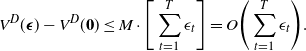 \begin{eqnarray}V^D(\boldsymbol{\epsilon}) - V^D(\textbf{0}) \le M \cdot \Bigg[\sum_{t=1}^T \epsilon_t\Bigg] = O\Bigg(\sum_{t=1}^T \epsilon_t\Bigg). \end{eqnarray}
The above lemma is used to prove Theorems 1–2 and Propositions 1–3 in Sections 4 and 6 of [Reference Zayas-Cabán, Jasin and Wang1]. It has been graciously pointed out to us that the bound in the lemma may not be correct in general. The original proof of this lemma uses a combination of linear program (LP) duality and sensitivity analysis results. The mistake is in the application of a known sensitivity analysis result under a certain assumption that happens to be not necessarily satisfied by our LP. Fortunately, it is possible to correct the bound in the above lemma. The new bound that we will prove in this correction note is as follows:
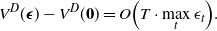 \begin{eqnarray}V^D(\boldsymbol{\epsilon}) - V^D(\textbf{0}) = O\Big(T \cdot \max_t \epsilon_t\Big). \end{eqnarray}
In what follows, we will provide enough discussion so that the correctness of (2) can be easily verified. In Section 2, we recall the complete definition of the LP with both discounting factor and bandit arrivals that was used in [Reference Zayas-Cabán, Jasin and Wang1]. In Section 3, we provide a formal statement of the new lemma and its proof. In Section 4, we discuss how this new bound affects the results in subsequent theorems and propositions in [1].
2. The linear program
Recall that the original bound (1) was used to prove the results in Sections 4 and 6 of [Reference Zayas-Cabán, Jasin and Wang1]. In [Reference Zayas-Cabán, Jasin and Wang1, Section 4] we analyzed a ‘fixed population’ model, while in [Reference Zayas-Cabán, Jasin and Wang1, Section 6] we analyzed the more general ‘dynamic population’ model where bandits can arrive in, or depart from, the system. Since the LP used in [Reference Zayas-Cabán, Jasin and Wang1, Section 6] is a generalization of the LP used in [Reference Zayas-Cabán, Jasin and Wang1, Section 4], we only present our analysis for the general LP used in [Reference Zayas-Cabán, Jasin and Wang1, Section 6]. The definition of the LP for any discount factor $\delta \in [0,1]$
and
$\delta \in [0,1]$
and $\boldsymbol{\epsilon} = (\epsilon_1, \dots, \epsilon_T) \ge \textbf{0}$
is given by
$\boldsymbol{\epsilon} = (\epsilon_1, \dots, \epsilon_T) \ge \textbf{0}$
is given by
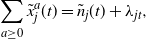
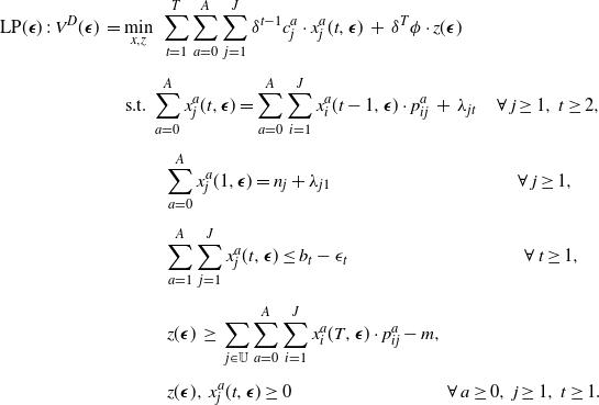 \begin{eqnarray}\mbox{LP}({\boldsymbol{\epsilon}})\;:\; V^D(\boldsymbol{\epsilon}) \, = &&\; \min_{x, z} \,\, \sum_{t = 1}^T \sum_{a=0}^A \sum_{j = 1}^{J} \delta^{t-1} c_{j}^a \cdot x_{j}^a(t, \boldsymbol{\epsilon}) \, + \, \delta^{T} \phi \cdot z(\boldsymbol{\epsilon}) \\[5pt] && \mbox{ s.t. } \sum_{a=0}^{A} x_{j}^a(t, \boldsymbol{\epsilon}) = \sum_{a=0}^A \sum_{i=1}^{J} x_{i}^a(t-1, \boldsymbol{\epsilon}) \cdot p^a_{ij} \, + \, \lambda_{jt} \hspace{4mm} \forall \, j\ge 1 , \, t \ge 2, \nonumber \\[5pt] && \hspace{9mm} \sum_{a = 0}^A x_{j}^{a} (1, \boldsymbol{\epsilon}) = n_{j} + \lambda_{j1} \hspace{36mm} \forall \, j \ge 1, \nonumber \\[5pt] && \hspace{9mm} \sum_{a=1}^A \sum_{j=1}^J x^a_j(t, \boldsymbol{\epsilon}) \le b_t - \epsilon_t \hspace{34mm} \forall \, t \ge 1, \nonumber \\[5pt] && \hspace{9mm} z(\boldsymbol{\epsilon}) \, \ge \, \sum_{j \in \mathbb{U}} \sum_{a=0}^A \sum_{i=1}^J x^a_i(T, \boldsymbol{\epsilon}) \cdot p^a_{ij} - m, \nonumber \\[5pt] && \hspace{9mm} z(\boldsymbol{\epsilon}), \, x^a_j(t, \boldsymbol{\epsilon}) \ge 0 \hspace{30mm} \forall \, a \ge 0, \, j \ge 1, \, t \ge 1. \nonumber\end{eqnarray}
The decision variables in the above LP are the x’s and z. It is not difficult to see that the optimal solution will satisfy $z(\boldsymbol{\epsilon}) = \big(\sum_{j \in \mathbb{U}} \sum_{a=0}^A \sum_{i=1}^J x^a_i(T, \boldsymbol{\epsilon}) \cdot p^a_{ij} - m \big)^+$
. All parameters in the above LP are non-negative. In particular,
$z(\boldsymbol{\epsilon}) = \big(\sum_{j \in \mathbb{U}} \sum_{a=0}^A \sum_{i=1}^J x^a_i(T, \boldsymbol{\epsilon}) \cdot p^a_{ij} - m \big)^+$
. All parameters in the above LP are non-negative. In particular, $p^a_{ij}$
is the probability of transitioning from state i to state j under action a
$p^a_{ij}$
is the probability of transitioning from state i to state j under action a $\big(\textrm{i.e.,}\;\sum_j p^a_{ij} = 1$
for all a and i
$\big(\textrm{i.e.,}\;\sum_j p^a_{ij} = 1$
for all a and i $\big)$
,
$\big)$
, $\lambda_{jt}$
is the arrival rate (or expected number) of new bandits in state j at time t, and
$\lambda_{jt}$
is the arrival rate (or expected number) of new bandits in state j at time t, and $b_t$
is the activation budget at time t. The value of
$b_t$
is the activation budget at time t. The value of $\epsilon_t$
is assumed to be small enough so that
$\epsilon_t$
is assumed to be small enough so that $b_t - \epsilon_t \ge 0$
; otherwise, the LP is not feasible. In [Reference Zayas-Cabán, Jasin and Wang1, Section 3], we used
$b_t - \epsilon_t \ge 0$
; otherwise, the LP is not feasible. In [Reference Zayas-Cabán, Jasin and Wang1, Section 3], we used $\lambda_{jt} = 0$
for all j and t, and the bound in (1) was originally proved for this case. We did not provide the proof for the more general case where
$\lambda_{jt} = 0$
for all j and t, and the bound in (1) was originally proved for this case. We did not provide the proof for the more general case where $\lambda_{jt}$
could be positive, as the proof for this case was originally deemed to be a straightforward extension of the proof for the simpler case. To avoid confusion, below we will prove the new bound (2) for the general case where
$\lambda_{jt}$
could be positive, as the proof for this case was originally deemed to be a straightforward extension of the proof for the simpler case. To avoid confusion, below we will prove the new bound (2) for the general case where $\lambda_{jt}$
can also be positive.
$\lambda_{jt}$
can also be positive.
3. The new lemma
We state our new lemma.
Lemma 1.
Let $c_{\max} = \max_{a,j} c^a_j$
,
$c_{\max} = \max_{a,j} c^a_j$
, $b_{\max} = \max_t b_t$
,
$b_{\max} = \max_t b_t$
, $b_{\min} = \min_{t | b_t \neq 0} b_t$
, and
$b_{\min} = \min_{t | b_t \neq 0} b_t$
, and $\epsilon_{\max} = \max_t \epsilon_t$
. Let
$\epsilon_{\max} = \max_t \epsilon_t$
. Let $ \mathbb{1}_{\delta \neq 1}$
and
$ \mathbb{1}_{\delta \neq 1}$
and $ \mathbb{1}_{\delta = 1}$
be indicators for the cases
$ \mathbb{1}_{\delta = 1}$
be indicators for the cases $\delta \not= 1$
and
$\delta \not= 1$
and $\delta = 1$
, respectively. If
$\delta = 1$
, respectively. If $\epsilon_{\max} \le b_{\min}$
, then we have the following bound:
$\epsilon_{\max} \le b_{\min}$
, then we have the following bound:
 \begin{eqnarray*}&& V^D(\boldsymbol{\epsilon}) - V^D(\textbf{0}) \\[5pt]&&\quad \le c_{\max} \cdot \epsilon_{\max } \cdot \frac{ b_{\max}}{b_{\min}} \cdot \bigg[\bigg(\frac{1-\delta^T}{1-\delta}\bigg) \cdot \mathbb{1}_{\delta \neq 1} + T \cdot \mathbb{1}_{\delta = 1}\bigg] + 2 \delta^T \phi \cdot \epsilon_{\max } \cdot \frac{ b_{\max}}{b_{\min}}.\end{eqnarray*}
Proof. The proof is by construction. Let $\big\{x^a_j(t, \textbf{0})\big\}$
denote an optimal solution of LP(
$\big\{x^a_j(t, \textbf{0})\big\}$
denote an optimal solution of LP( $\textbf{0}$
). We will use
$\textbf{0}$
). We will use $\big\{x^a_j(t, \textbf{0})\big\}$
to construct a feasible solution
$\big\{x^a_j(t, \textbf{0})\big\}$
to construct a feasible solution $\big\{\tilde{x}^a_j(t, \boldsymbol{\epsilon})\big\}$
for LP(
$\big\{\tilde{x}^a_j(t, \boldsymbol{\epsilon})\big\}$
for LP( $\boldsymbol{\epsilon}$
), under which we let
$\boldsymbol{\epsilon}$
), under which we let $\tilde{z}(\boldsymbol{\epsilon}) = \big(\sum_{j \in \mathbb{U}} \sum_{a=0}^A \sum_{i=1}^J \tilde{x}^a_i(T, \boldsymbol{\epsilon}) \cdot p^a_{ij} - m \big)^+$
be the feasible z variable, and show that the gap between the objective value of LP(
$\tilde{z}(\boldsymbol{\epsilon}) = \big(\sum_{j \in \mathbb{U}} \sum_{a=0}^A \sum_{i=1}^J \tilde{x}^a_i(T, \boldsymbol{\epsilon}) \cdot p^a_{ij} - m \big)^+$
be the feasible z variable, and show that the gap between the objective value of LP( $\boldsymbol{\epsilon}$
) under
$\boldsymbol{\epsilon}$
) under $\big\{\tilde{x}^a_j(t, \boldsymbol{\epsilon})\big\}$
and
$\big\{\tilde{x}^a_j(t, \boldsymbol{\epsilon})\big\}$
and $V^D(\textbf{0})$
satisfies the bound in Lemma 1.
$V^D(\textbf{0})$
satisfies the bound in Lemma 1.
For ease of exposition, we will write $x^a_j(t, \textbf{0})$
as
$x^a_j(t, \textbf{0})$
as $x^a_j(t)$
and
$x^a_j(t)$
and $\tilde{x}^a_j(t, \boldsymbol{\epsilon})$
as
$\tilde{x}^a_j(t, \boldsymbol{\epsilon})$
as $\tilde{x}^a_j(t)$
. Define
$\tilde{x}^a_j(t)$
. Define $t^*=\arg\max_{\{t | b_t \neq 0\}} \frac{\epsilon_{t}}{b_{t}}$
and let
$t^*=\arg\max_{\{t | b_t \neq 0\}} \frac{\epsilon_{t}}{b_{t}}$
and let $\beta \in [0,1] $
be such that
$\beta \in [0,1] $
be such that
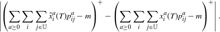
 \begin{eqnarray} (1-\beta) \cdot b_t \ge \epsilon_{t} \hspace{2cm}\forall t\in [T].\end{eqnarray}
In our construction of $\big\{\tilde x_j^a(t)\big\}$
shortly, we will see that the term
$\big\{\tilde x_j^a(t)\big\}$
shortly, we will see that the term $\beta b_t$
can be interpreted as an upper bound of total budget consumption at time t
$\beta b_t$
can be interpreted as an upper bound of total budget consumption at time t $\big($
i.e.,
$\big($
i.e., $\sum_{a=1}^A \sum_{j=1}^J \tilde{x}^a_j(t)\big).$
In particular, we use the following value of
$\sum_{a=1}^A \sum_{j=1}^J \tilde{x}^a_j(t)\big).$
In particular, we use the following value of $\beta$
:
$\beta$
:
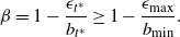 \begin{eqnarray}\beta = 1- \frac{\epsilon_{t^*}}{b_{t^*}}\ge 1- \frac{\epsilon_{\max}}{b_{\min}}. \end{eqnarray}
Let $\boldsymbol{\gamma} = (\gamma_1, \gamma_2 \dots \gamma_T)$
, where
$\boldsymbol{\gamma} = (\gamma_1, \gamma_2 \dots \gamma_T)$
, where $\gamma_t= (1-\beta) \cdot b_t$
. Note that, by definition of
$\gamma_t= (1-\beta) \cdot b_t$
. Note that, by definition of $\gamma_t$
, we have
$\gamma_t$
, we have
 \begin{eqnarray*} \gamma_t \, \le \, \frac{\epsilon_{\max}}{b_{\min}}\cdot b_t \, \le \, \epsilon_{\max}\cdot \frac{b_{\max}}{b_{\min}} \end{eqnarray*}
for any t.
We now discuss the construction of $\big\{\tilde{x}^a_j(t)\big\}$
. We first describe the construction for
$\big\{\tilde{x}^a_j(t)\big\}$
. We first describe the construction for $t=1$
and then complete the construction for
$t=1$
and then complete the construction for $t \ge 2$
by induction. For
$t \ge 2$
by induction. For $t = 1$
, define
$t = 1$
, define $\big\{\tilde{x}^a_j(1)\big\}$
as follows:
$\big\{\tilde{x}^a_j(1)\big\}$
as follows:
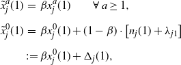 \begin{eqnarray*}\tilde{x}^a_j(1) &=& \beta x^a_j(1) \qquad \forall \, a \ge 1, \\[5pt]\tilde{x}^0_j(1) &=& \beta x^0_j(1) + (1-\beta) \cdot \big[ n_j(1) + \lambda_{j1} \big] \\[5pt] & \;:\!=\;& \beta x^0_j(1) + \Delta_j (1),\end{eqnarray*}
where $\Delta_j(1) = (1-\beta) \cdot \left[ n_j(1) + \lambda_{j1} \right]$
. Clearly,
$\Delta_j(1) = (1-\beta) \cdot \left[ n_j(1) + \lambda_{j1} \right]$
. Clearly, $\tilde{x}^a_j(1) \ge 0$
and so
$\tilde{x}^a_j(1) \ge 0$
and so $\big\{\tilde{x}^a_j(1)\big\}$
satisfies the non-negativity constraint in LP(
$\big\{\tilde{x}^a_j(1)\big\}$
satisfies the non-negativity constraint in LP( $\boldsymbol{\epsilon}$
). It is also not difficult to see that
$\boldsymbol{\epsilon}$
). It is also not difficult to see that $\sum_{a \ge 0} \tilde{x}^a_j(1) = n_j(1) + \lambda_{j1}$
(because
$\sum_{a \ge 0} \tilde{x}^a_j(1) = n_j(1) + \lambda_{j1}$
(because $\sum_{a\ge 0} x^a_j(1) = n_j(1) + \lambda_{j1}$
, as
$\sum_{a\ge 0} x^a_j(1) = n_j(1) + \lambda_{j1}$
, as $\big\{x^a_j(t)\big\}$
is feasible for LP(
$\big\{x^a_j(t)\big\}$
is feasible for LP( $\textbf{0}$
)), and so
$\textbf{0}$
)), and so $\big\{\tilde{x}^a_j(1)\big\}$
satisfies the second constraint in LP(
$\big\{\tilde{x}^a_j(1)\big\}$
satisfies the second constraint in LP( $\boldsymbol{\epsilon}$
). Moreover, by definition of
$\boldsymbol{\epsilon}$
). Moreover, by definition of $\beta$
and
$\beta$
and $\gamma_1$
, we have
$\gamma_1$
, we have
 \begin{eqnarray*}\sum_{a \ge 1} \sum_i \tilde{x}^a_i(1) = \beta \cdot \Bigg[\sum_{a \ge 1} \sum_i x^a_i(1) \Bigg]\le \beta b_1 = b_1-\gamma_1 \le b_1-\epsilon_1,\end{eqnarray*}
so that $\big\{\tilde{x}^a_j(1)\big\}$
satisfies the ‘budget constraint’ (i.e., the third constraint) in LP
$\big\{\tilde{x}^a_j(1)\big\}$
satisfies the ‘budget constraint’ (i.e., the third constraint) in LP $(\boldsymbol{\epsilon})$
.
$(\boldsymbol{\epsilon})$
.
Before we proceed with the construction of $\big\{\tilde{x}^a_j(t)\big\}$
for
$\big\{\tilde{x}^a_j(t)\big\}$
for $t \ge 2$
, we define
$t \ge 2$
, we define $n_j(t)$
and
$n_j(t)$
and $\tilde{n}_j(t)$
as follows:
$\tilde{n}_j(t)$
as follows:
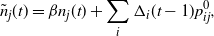
 \begin{eqnarray*}n_j(t) = \sum_{a \ge 0} \sum_i x^a_i(t-1) p^a_{ij} \,\,\, \mbox{ and } \,\,\, \tilde{n}_j(t) = \sum_{a \ge 0} \sum_i \tilde{x}^a_i(t-1) p^a_{ij}.\end{eqnarray*}
For $t \geq 2$
, we define
$t \geq 2$
, we define $\Delta_j(t)$
and
$\Delta_j(t)$
and $\big\{\tilde{x}^a_j(t)\big\}$
recursively as follows:
$\big\{\tilde{x}^a_j(t)\big\}$
recursively as follows:
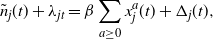
 \begin{align*} \Delta_j(t) & =\sum_i \Delta_i(t-1)\cdot p^0_{ij} + (1-\beta) \lambda_{jt}, \\[5pt]\tilde{x}^a_j(t) & = \beta x^a_j(t) \qquad \forall \, a \ge 1, \\[5pt]\tilde{x}^0_j(t)&= \beta x^0_j(t) +\Delta_j(t). \end{align*}
We prove the following identities by induction:
 \begin{eqnarray}\tilde{n}_j(t) = \beta n_j(t) + \sum_i \Delta_i(t-1) p^0_{ij},\end{eqnarray}
 \begin{eqnarray}\tilde{n}_j(t) + \lambda_{jt} = \beta \sum_{a\ge 0} x_j^a(t) + \Delta_j (t),\end{eqnarray}
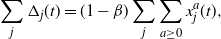 \begin{eqnarray}\sum_{j}\Delta_j(t) = (1-\beta) \sum_j \sum_{a\ge 0} x_j^a(t),\end{eqnarray}
 \begin{eqnarray}\sum_{a \ge 0} \tilde{x}^a_j(t) = \tilde{n}_j(t) + \lambda_{jt},\end{eqnarray}
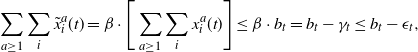 \begin{eqnarray}\sum_{a \ge 1} \sum_i \tilde{x}^a_i(t) = \beta \cdot \Bigg[\sum_{a \ge 1} \sum_i x^a_i(t) \Bigg] \le \beta \cdot b_t = b_t-\gamma_t \le b_t - \epsilon_t,\end{eqnarray}
 \begin{eqnarray}\sum_{j}\Big[ \tilde{x}^0_j(t) -{x}^0_j(t) \Big] = (1-\beta) \sum_j \sum_{a\ge 1} x_j ^a (t) \le (1-\beta) b_t = \gamma_t.\end{eqnarray}
First note that Equation (6) follows directly from the definition of $\tilde{n}_j(t)$
and
$\tilde{n}_j(t)$
and $\big\{\tilde{x}^a_j(t)\big\}$
:
$\big\{\tilde{x}^a_j(t)\big\}$
:
 \begin{eqnarray*}\tilde{n}_j(t) = \sum_{a \ge 0} \sum_i \tilde{x}^a_i(t-1) p^a_{ij} = \beta n_j(t) + \sum_i \Delta_i(t-1) p^0_{ij}.\end{eqnarray*}
Next, Equation (7) follows from (6) and the fact that $\sum_{a \ge 0} x^a_j(t) = n_j(t) + \lambda_{jt}$
(because
$\sum_{a \ge 0} x^a_j(t) = n_j(t) + \lambda_{jt}$
(because $\big\{x^a_j(t)\big\}$
is feasible for LP(
$\big\{x^a_j(t)\big\}$
is feasible for LP( $\textbf{0}$
)):
$\textbf{0}$
)):
 \begin{align*}\tilde{n}_j(t) + \lambda_{jt} &= \beta n_j(t) + \sum_i \Delta_i(t-1) p^0_{ij} + \lambda_{jt} \\[5pt] &= \beta [n_j(t) + \lambda_{jt}] + \Bigg[\sum_i \Delta_i(t-1) p^0_{ij} + (1-\beta) \lambda_{jt}\Bigg] \\[5pt] &= \beta [n_j(t) + \lambda_{jt}] + \Delta_j(t) \\[5pt] &= \beta \sum_{a \ge 0} x^a_j(t) + \Delta_j(t).\end{align*}
Equation (9) follows directly from the definition of $\big\{\tilde{x}^a_j(t)\big\}$
and (7), whereas Equation (10) follows from the definition of
$\big\{\tilde{x}^a_j(t)\big\}$
and (7), whereas Equation (10) follows from the definition of $\big\{\tilde{x}^a_j(t)\big\}$
and the fact that
$\big\{\tilde{x}^a_j(t)\big\}$
and the fact that $\sum_j \sum_{a\ge 1} x_j ^a (t) \le b_t$
(because
$\sum_j \sum_{a\ge 1} x_j ^a (t) \le b_t$
(because $\big\{x^a_j(t)\big\}$
is feasible for LP(
$\big\{x^a_j(t)\big\}$
is feasible for LP( $\textbf{0}$
)). Equation (11) follows from the definition of
$\textbf{0}$
)). Equation (11) follows from the definition of $\big\{\tilde{x}^a_j(t)\big\}$
together with (8) and the fact that
$\big\{\tilde{x}^a_j(t)\big\}$
together with (8) and the fact that $\sum_j \sum_{a\ge 1} x_j ^a (t) \le b_t$
. Thus, among the six identities (6)–(11), we only need to show (8) by induction. Note that Equations (9) and (10) imply that the constructed
$\sum_j \sum_{a\ge 1} x_j ^a (t) \le b_t$
. Thus, among the six identities (6)–(11), we only need to show (8) by induction. Note that Equations (9) and (10) imply that the constructed $\big\{\tilde{x}^a_j(t)\big\}$
for
$\big\{\tilde{x}^a_j(t)\big\}$
for $t \ge 2$
satisfies the first and third constraints in LP(
$t \ge 2$
satisfies the first and third constraints in LP( $\boldsymbol{\epsilon}$
). Since
$\boldsymbol{\epsilon}$
). Since $\tilde{x}^a_{j}(t)$
is obviously non-negative by construction, it also satisfies the non-negative constraint. As a result, the constructed
$\tilde{x}^a_{j}(t)$
is obviously non-negative by construction, it also satisfies the non-negative constraint. As a result, the constructed $\big\{\tilde{x}^a_j(t)\big\}$
is feasible for LP(
$\big\{\tilde{x}^a_j(t)\big\}$
is feasible for LP( $\boldsymbol{\epsilon}$
).
$\boldsymbol{\epsilon}$
).
We prove (8) by induction starting with $t = 2$
. By definition of
$t = 2$
. By definition of $\Delta_j(2)$
,
$\Delta_j(2)$
,
 \begin{align*}\sum_j \Delta_j(2) &=\sum_j \Bigg[ \sum_i \Delta_{i}(1) p^0_{ij} +(1-\beta) \lambda_{j,2} \Bigg] \\[5pt]&= \sum_i \Delta_{i}(1) +(1-\beta)\sum_j \lambda_{j,2} \\[5pt]&= (1-\beta) \Bigg[\sum_i \sum_{a \ge 0} x^a_i(1) +\sum_j \lambda_{j,2} \Bigg]\\[5pt]&= (1-\beta) \Bigg[ \sum_{j} n_j (2) + \sum_j \lambda_{j,2} \Bigg]\\[5pt]&= (1-\beta) \sum_j \big[ n_j (2) + \lambda_{j,2} \big]\\[5pt]&= (1-\beta) \sum_j \sum_{a\ge 0} x_j^a(2),\end{align*}
where the third equality follows since, by definition, $\Delta_i(1) = (1-\beta) [n_i(1) + \lambda_{i,1}] = (1 - \beta) \sum_{a \ge 0} x^a_i(1)$
(from the second constraint in LP(
$\Delta_i(1) = (1-\beta) [n_i(1) + \lambda_{i,1}] = (1 - \beta) \sum_{a \ge 0} x^a_i(1)$
(from the second constraint in LP( $\textbf{0}$
)); the fourth equality follows by the definition of
$\textbf{0}$
)); the fourth equality follows by the definition of $n_j(2)$
; and the last equality follows by the first constraint in LP(
$n_j(2)$
; and the last equality follows by the first constraint in LP( $\textbf{0}$
).
$\textbf{0}$
).
Now, suppose that (6)–(11) hold for all times $s \le t$
. Then
$s \le t$
. Then
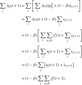 \begin{align*}\sum_{j}\Delta_j(t+1) &=\sum_j \Bigg[ \sum_i \Delta_i(t) p^0_{ij} + (1-\beta) \lambda_{j,t+1} \Bigg]\\[5pt] &= \sum_i \Delta_i(t) + (1-\beta) \sum_j \lambda_{j,t+1} \\[5pt] &= (1-\beta) \Bigg[\sum_i \sum_{a \ge 0} x^a_i(t) +\sum_j \lambda_{j,t+1} \Bigg]\\[5pt]&= (1-\beta) \Bigg[ \sum_{j} n_j (t+1) + \sum_j \lambda_{j,t+1} \Bigg]\\[5pt]&= (1-\beta) \sum_j \big[ n_j (t+1) + \lambda_{j,t + 1} \big]\\[5pt]&= (1-\beta) \sum_j \sum_{a\ge 0} x_j^a(t+1),\end{align*}
where the third equality follows by the induction hypothesis, the fourth equality follows by the definition of $n_j(t)$
, and the last equality follows by the first constraint in LP(
$n_j(t)$
, and the last equality follows by the first constraint in LP( $\textbf{0}$
). This completes our inductive step and thus the proof by induction.
$\textbf{0}$
). This completes our inductive step and thus the proof by induction.
We have so far shown that the constructed $\big\{\tilde{x}^a_j(t)\big\}$
is feasible for LP
$\big\{\tilde{x}^a_j(t)\big\}$
is feasible for LP $(\boldsymbol{\epsilon})$
. We now compute a bound for
$(\boldsymbol{\epsilon})$
. We now compute a bound for $V^D(\boldsymbol{\epsilon}) - V^D(\textbf{0})$
. Let
$V^D(\boldsymbol{\epsilon}) - V^D(\textbf{0})$
. Let $V^D(\boldsymbol{\epsilon}, \tilde{x})$
denote the objective value of LP
$V^D(\boldsymbol{\epsilon}, \tilde{x})$
denote the objective value of LP $(\boldsymbol{\epsilon})$
under
$(\boldsymbol{\epsilon})$
under $\big\{\tilde{x}^a_j(t)\big\}$
. Then
$\big\{\tilde{x}^a_j(t)\big\}$
. Then $V^D(\boldsymbol{\epsilon}) - V^D(\textbf{0}) \le V^D(\boldsymbol{\epsilon}, \tilde{x}) - V^D(\textbf{0})$
. Now,
$V^D(\boldsymbol{\epsilon}) - V^D(\textbf{0}) \le V^D(\boldsymbol{\epsilon}, \tilde{x}) - V^D(\textbf{0})$
. Now,
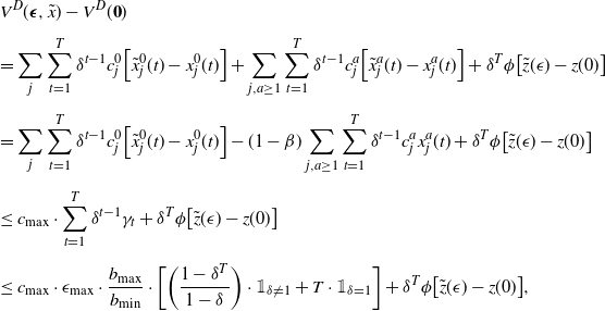 \begin{eqnarray*}&& V^D(\boldsymbol{\epsilon}, \tilde{x}) - V^D(\textbf{0}) \\[5pt] &&= \sum_j\sum_{t=1}^T \delta^{t-1} c_j^0 \Big[ \tilde x_j^0(t)-x_j^0(t)\Big] + \sum_{j, a \ge 1} \sum_{t=1}^T \delta^{t-1} c_j^a \Big[ \tilde x_j^a(t)-x_j^a(t)\Big]+ \delta^T \phi \big[\tilde{z}(\epsilon )-z(0 )\big] \\[5pt]&&=\sum_j\sum_{t=1}^T \delta^{t-1} c_j^0 \Big[ \tilde x_j^0(t)-x_j^0(t)\Big] -(1-\beta) \sum_{j, a\ge 1} \sum_{t=1}^T \delta^{t-1} c^a_j x_j^a(t) + \delta^T \phi \big[\tilde{z}(\epsilon )-z(0 )\big] \\[5pt]&&\le c_{\max} \cdot \sum_{t=1}^T \delta^{t-1} \gamma_t + \delta^T \phi \big[\tilde{z}(\epsilon )-z(0 )\big] \\[5pt] &&\le c_{\max} \cdot \epsilon_{\max } \cdot \frac{ b_{\max}}{b_{\min}} \cdot \bigg[\bigg(\frac{1-\delta^T}{1-\delta}\bigg) \cdot \mathbb{1}_{\delta \neq 1} + T \cdot \mathbb{1}_{\delta = 1}\bigg] + \delta^T \phi \big[\tilde{z}(\epsilon )-z(0 )\big],\end{eqnarray*}
where the first inequality follows from (11) and the last inequality follows since $\gamma_t \le \epsilon_{\max } \cdot b_{\max}/b_{\min}$
. It remains to bound
$\gamma_t \le \epsilon_{\max } \cdot b_{\max}/b_{\min}$
. It remains to bound $\delta^T \phi [\tilde{z}(\epsilon )-z(0 )]$
.
$\delta^T \phi [\tilde{z}(\epsilon )-z(0 )]$
.
To this end, recall that
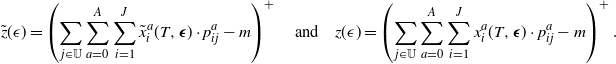 \begin{align*} \tilde{z}(\epsilon) = \left(\sum_{j \in \mathbb{U}} \sum_{a=0}^A \sum_{i=1}^J \tilde{x}^a_i(T, \boldsymbol{\epsilon}) \cdot p^a_{ij} - m \right)^+ \quad \text{and} \quad z(\epsilon) = \left(\sum_{j \in \mathbb{U}} \sum_{a=0}^A \sum_{i=1}^J x^a_i(T, \boldsymbol{\epsilon}) \cdot p^a_{ij} - m \right)^+.\end{align*}
Since $\epsilon=0$
corresponds to the optimal LP solution,
$\epsilon=0$
corresponds to the optimal LP solution, $z(0)=(\sum_{j \in \mathbb{U}} \sum_{a=0}^A \sum_{i=1}^J x^a_i(T) \cdot p^a_{ij} - m )^+$
. Next, recall that
$z(0)=(\sum_{j \in \mathbb{U}} \sum_{a=0}^A \sum_{i=1}^J x^a_i(T) \cdot p^a_{ij} - m )^+$
. Next, recall that $\epsilon$
corresponds to perturbing the original LP and as such represents a generalization of this original LP. It follows that
$\epsilon$
corresponds to perturbing the original LP and as such represents a generalization of this original LP. It follows that $\tilde{z}(\epsilon ) \leq \tilde{z}(0)=(\sum_{j \in \mathbb{U}} \sum_{a=0}^A \sum_{i=1}^J \tilde{x}^a_i(T) \cdot p^a_{ij} - m )^+$
. From this it follows that
$\tilde{z}(\epsilon ) \leq \tilde{z}(0)=(\sum_{j \in \mathbb{U}} \sum_{a=0}^A \sum_{i=1}^J \tilde{x}^a_i(T) \cdot p^a_{ij} - m )^+$
. From this it follows that $\tilde{z}(\epsilon )-z(0 )$
is bounded above by
$\tilde{z}(\epsilon )-z(0 )$
is bounded above by
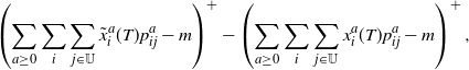 \begin{align*} \left(\sum_{a \ge 0} \sum_i \sum_{j \in \mathbb{U}} \tilde{x}^a_i(T) p^a_{ij} - m \right)^+ - \left(\sum_{a \ge 0} \sum_i \sum_{j \in \mathbb{U}} x^a_i(T) p^a_{ij} - m\right)^+,\end{align*}
and this last expression is bounded above by
 \begin{align*} \left|\left(\sum_{a \ge 0} \sum_i \sum_{j \in \mathbb{U}} \tilde{x}^a_i(T) p^a_{ij} - m \right)^+ - \left(\sum_{a \ge 0} \sum_i \sum_{j \in \mathbb{U}} x^a_i(T) p^a_{ij} - m\right)^+\right|.\end{align*}
Applying the property $\max\{a,b\}= \frac{1}{2}\left(a+b+|a-b|\right)$
, where a and b are arbitrary real numbers, yields
$\max\{a,b\}= \frac{1}{2}\left(a+b+|a-b|\right)$
, where a and b are arbitrary real numbers, yields
 \begin{align*} \left(\sum_{a \ge 0} \sum_i \sum_{j \in \mathbb{U}} \tilde{x}^a_i(T) p^a_{ij} - m \right)^+ = \max \left\{\sum_{a \ge 0} \sum_i \sum_{j \in \mathbb{U}} \tilde{x}^a_i(T) p^a_{ij} - m ,0 \right\} \\[5pt] \quad = \frac{1}{2}\left(\sum_{a \ge 0} \sum_i \sum_{j \in \mathbb{U}} \tilde{x}^a_i(T) p^a_{ij} - m + \left| \sum_{a \ge 0} \sum_i \sum_{j \in \mathbb{U}} \tilde{x}^a_i(T) p^a_{ij} - m \right|\right)\end{align*}
and
 \begin{align*} \left(\sum_{a \ge 0} \sum_i \sum_{j \in \mathbb{U}} x^a_i(T) p^a_{ij} - m \right)^+ = \max \left\{\sum_{a \ge 0} \sum_i \sum_{j \in \mathbb{U}} x^a_i(T) p^a_{ij} - m,0 \right\} \\[5pt] \quad = \frac{1}{2}\left(\sum_{a \ge 0} \sum_i \sum_{j \in \mathbb{U}} x^a_i(T) p^a_{ij} - m + \left|\sum_{a \ge 0} \sum_i \sum_{j \in \mathbb{U}} x^a_i(T) p^a_{ij} - m \right|\right).\end{align*}
Since $|a-b| \geq |a|-|b|$
and, similarly,
$|a-b| \geq |a|-|b|$
and, similarly, $|b-a|=|a-b| \geq |b| - |a| = -(|a|-|b|)$
for any two real numbers a and b, the last calculation yields that the expression
$|b-a|=|a-b| \geq |b| - |a| = -(|a|-|b|)$
for any two real numbers a and b, the last calculation yields that the expression
 \begin{align*} \left|\left(\sum_{a \ge 0} \sum_i \sum_{j \in \mathbb{U}} \tilde{x}^a_i(T) p^a_{ij} - m \right)^+ - \left(\sum_{a \ge 0} \sum_i \sum_{j \in \mathbb{U}} x^a_i(T) p^a_{ij} - m\right)^+\right|\end{align*}
is bounded above by
 \begin{align*} \left|\sum_{a \ge 0} \sum_i \sum_{j \in \mathbb{U}} \tilde{x}^a_i(T) p^a_{ij} - \sum_{a \ge 0} \sum_i \sum_{j \in \mathbb{U}} x^a_i(T) p^a_{ij} \right|.\end{align*}
The triangle inequality then implies that this last expression is bounded above by
 \begin{align*} \left|\sum_{i, a \ge 1} \sum_{j \in \mathbb{U}} \tilde{x}^a_i(T) p^a_{ij} - \sum_{i, a \ge 1} \sum_{j \in \mathbb{U}} x^a_i(T) p^a_{ij}\right| + \left|\sum_i \sum_{j \in \mathbb{U}} \tilde{x}^0_i(T) p^0_{ij} - \sum_i \sum_{j \in \mathbb{U}} x^0_i(T) p^a_{ij}\right|.\end{align*}
The property (10) implies that the terms inside the first set of absolute values equals $(1-\beta) \sum_{a \geq 1} \sum_i \sum_{j \in U} x^a_i(T) p^a_{ij}$
, so that the expression above equals
$(1-\beta) \sum_{a \geq 1} \sum_i \sum_{j \in U} x^a_i(T) p^a_{ij}$
, so that the expression above equals
 \begin{align*} (1-\beta) \sum_{a \ge 1} \sum_i \sum_{j \in \mathbb{U}} x^a_i(T) p^a_{ij} + \left|\sum_i \sum_{j \in \mathbb{U}} \tilde{x}^0_i(T) p^0_{ij} - \sum_i \sum_{j \in \mathbb{U}} x^0_i(T) p^0_{ij}\right|,\end{align*}
which is bounded above by
 \begin{align*} (1-\beta) \sum_{a \ge 1} \sum_i \sum_{j} x^a_i(T) p^a_{ij} + \left|\sum_i \sum_{j \in \mathbb{U}} \tilde{x}^0_i(T) p^0_{ij} - \sum_i \sum_{j \in \mathbb{U}} x^0_i(T) p^0_{ij}\right|,\end{align*}
which, by (10), equals
 \begin{align*} (1-\beta) \sum_{a \ge 1} \sum_i x^a_i(T) + (1-\beta) \sum_{j \in \mathbb{U}} \sum_i \sum_{a\ge 1} x^a_i(T) p^0_{ij}.\end{align*}
This last expression is bounded above by $2 (1-\beta) \sum_{a \ge 1} \sum_i x^a_i(T) \le 2 (1-\beta) b_T \leq 2 \gamma_T$
. The choice of
$2 (1-\beta) \sum_{a \ge 1} \sum_i x^a_i(T) \le 2 (1-\beta) b_T \leq 2 \gamma_T$
. The choice of $\beta$
and definition of
$\beta$
and definition of $\gamma_T$
yield that
$\gamma_T$
yield that $2 \gamma_T$
is bounded above by
$2 \gamma_T$
is bounded above by $2 \epsilon_{max} \cdot \frac{b_{max}}{b_{min}}$
, as claimed.
$2 \epsilon_{max} \cdot \frac{b_{max}}{b_{min}}$
, as claimed.
4. Impact on other results in Zayas-Cabán et al. (2019) [Reference Zayas-Cabán, Jasin and Wang1]
As noted earlier, the bound in the original version of [Reference Zayas-Cabán, Jasin and Wang1, Lemma 2] was used to prove Theorems 1–2 and Propositions 1–3 in Sections 4 and 6 of [Reference Zayas-Cabán, Jasin and Wang1]. It turns out that the new bound in Lemma 1 does not change the results of Theorem 1, Theorem 2, or Proposition 3, but it does slightly change the bounds in Propositions 1 and 2. We discuss all of these below.
Theorem 1 in [Reference Zayas-Cabán, Jasin and Wang1, Section 4]. In this theorem, we consider the setting where $\lambda_{jt} = 0$
for all j and t, and
$\lambda_{jt} = 0$
for all j and t, and $\delta = 1$
. We can use exactly the same
$\delta = 1$
. We can use exactly the same $\epsilon_t$
as defined in the original version of [Reference Zayas-Cabán, Jasin and Wang1, Theorem 1]. By the new lemma (Lemma 1 of this paper), we still have
$\epsilon_t$
as defined in the original version of [Reference Zayas-Cabán, Jasin and Wang1, Theorem 1]. By the new lemma (Lemma 1 of this paper), we still have $V^D_{\theta}(\boldsymbol{\epsilon}) - V^D_{\theta}(\textbf{0}) = O(T\sqrt{d \cdot \theta \ln \theta})$
. As a result, there are no changes and we still get exactly the same bound as in the original Theorem 1.
$V^D_{\theta}(\boldsymbol{\epsilon}) - V^D_{\theta}(\textbf{0}) = O(T\sqrt{d \cdot \theta \ln \theta})$
. As a result, there are no changes and we still get exactly the same bound as in the original Theorem 1.
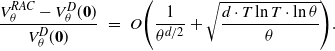
Proposition 1 in [Reference Zayas-Cabán, Jasin and Wang1, Section 4]. In this proposition, we consider the same setting considered in [Reference Zayas-Cabán, Jasin and Wang1, Theorem 1], with the exception that we set $\delta \in (0,1)$
. If we use the same
$\delta \in (0,1)$
. If we use the same $\epsilon_t$
as defined in the original [Reference Zayas-Cabán, Jasin and Wang1, Proposition 1], by the new Lemma 1 we have
$\epsilon_t$
as defined in the original [Reference Zayas-Cabán, Jasin and Wang1, Proposition 1], by the new Lemma 1 we have $V^D_{\theta}(\boldsymbol{\epsilon}) - V^D_{\theta}(\textbf{0}) = O(\sqrt{d \cdot \ln T \cdot \theta \ln \theta})$
(the original bound under the old Lemma 2 of [Reference Zayas-Cabán, Jasin and Wang1] was
$V^D_{\theta}(\boldsymbol{\epsilon}) - V^D_{\theta}(\textbf{0}) = O(\sqrt{d \cdot \ln T \cdot \theta \ln \theta})$
(the original bound under the old Lemma 2 of [Reference Zayas-Cabán, Jasin and Wang1] was $O(\sqrt{d \cdot \theta \ln \theta})$
). This implies that the new bound for [Reference Zayas-Cabán, Jasin and Wang1, Proposition 1] is given by
$O(\sqrt{d \cdot \theta \ln \theta})$
). This implies that the new bound for [Reference Zayas-Cabán, Jasin and Wang1, Proposition 1] is given by
 \begin{eqnarray*}\frac{V^{RAC}_{\theta} - V^D_{\theta}(\textbf{0})}{V^D_{\theta}(\textbf{0})} \,\, = \,\, O\Bigg(\frac{1}{\theta^d} + \sqrt{\frac{d \cdot \ln T \cdot \ln \theta}{\theta}}\Bigg).\end{eqnarray*}
Note that if we instead apply the same $\epsilon_t$
as defined in [Reference Zayas-Cabán, Jasin and Wang1, Theorem 1] to [Reference Zayas-Cabán, Jasin and Wang1, Proposition 1], it is not difficult to check that the bound becomes
$\epsilon_t$
as defined in [Reference Zayas-Cabán, Jasin and Wang1, Theorem 1] to [Reference Zayas-Cabán, Jasin and Wang1, Proposition 1], it is not difficult to check that the bound becomes
 \begin{eqnarray*}\frac{V^{RAC}_{\theta} - V^D_{\theta}(\textbf{0})}{V^D_{\theta}(\textbf{0})} \,\, = \,\, O\Bigg(\frac{T^2}{\theta^d} + \sqrt{\frac{d \cdot \ln \theta}{\theta}}\Bigg),\end{eqnarray*}
which, with a proper choice of d, essentially has the same order of magnitude as the bound in Theorem 1.
Theorem 2 in [Reference Zayas-Cabán, Jasin and Wang1, Section 6]. In this theorem, we consider the setting where $\lambda_{jt}$
could be positive, and
$\lambda_{jt}$
could be positive, and $\delta = 1$
. We can use exactly the same
$\delta = 1$
. We can use exactly the same $\epsilon_t$
as defined in the original version of [Reference Zayas-Cabán, Jasin and Wang1, Theorem 2]. By the new Lemma 1, we still have
$\epsilon_t$
as defined in the original version of [Reference Zayas-Cabán, Jasin and Wang1, Theorem 2]. By the new Lemma 1, we still have $V^D_{\theta}(\boldsymbol{\epsilon}) - V^D_{\theta}(\textbf{0}) = O(T^{3/2} \sqrt{d \cdot \theta \ln \theta})$
. As a result, nothing changes and we still get exactly the same bound as in the original Theorem 2.
$V^D_{\theta}(\boldsymbol{\epsilon}) - V^D_{\theta}(\textbf{0}) = O(T^{3/2} \sqrt{d \cdot \theta \ln \theta})$
. As a result, nothing changes and we still get exactly the same bound as in the original Theorem 2.
Proposition 2 in [Reference Zayas-Cabán, Jasin and Wang1, Section 6]. In this proposition, we consider the setting where $\lambda_{jt}$
may be positive and
$\lambda_{jt}$
may be positive and $\delta \in (0,1)$
. If we use the same
$\delta \in (0,1)$
. If we use the same $\epsilon_t$
as defined in the original version of [Reference Zayas-Cabán, Jasin and Wang1, Proposition 2], the new bound in Proposition 2 is given by
$\epsilon_t$
as defined in the original version of [Reference Zayas-Cabán, Jasin and Wang1, Proposition 2], the new bound in Proposition 2 is given by
 \begin{eqnarray*}\frac{V^{RAC}_{\theta} - V^D_{\theta}(\textbf{0})}{V^D_{\theta}(\textbf{0})} \,\, = \,\, O\Bigg(\frac{1}{\theta^{d/2}} + \sqrt{\frac{d \cdot T \ln T \cdot \ln \theta}{\theta}}\Bigg).\end{eqnarray*}
Proposition 3 in [Reference Zayas-Cabán, Jasin and Wang1, Section 6]. In this proposition, we consider the setting where bandits can complete service or abandon. Since $\alpha \in (0,1)$
, we have
$\alpha \in (0,1)$
, we have $\epsilon_{\max} = O\left(\sqrt{\frac{d \theta \ln \theta}{1 - \beta}}\right)$
. So, by the new Lemma 1,
$\epsilon_{\max} = O\left(\sqrt{\frac{d \theta \ln \theta}{1 - \beta}}\right)$
. So, by the new Lemma 1, $V^D_{\theta}(\boldsymbol{\epsilon}) - V^D_{\theta}(\textbf{0}) = O\left(T \sqrt{\frac{d \cdot \theta \ln \theta}{1-\beta}}\right)$
. This does not change anything in the proof of Proposition 3, and so the final bound in Proposition 3 also does not change.
$V^D_{\theta}(\boldsymbol{\epsilon}) - V^D_{\theta}(\textbf{0}) = O\left(T \sqrt{\frac{d \cdot \theta \ln \theta}{1-\beta}}\right)$
. This does not change anything in the proof of Proposition 3, and so the final bound in Proposition 3 also does not change.
