


1. Introduction
The power generation efficiency of magnetic confinement nuclear fusion reactors will be strongly dependent on the effective transfer of heat from the sidewall of the reactor chamber to the fluid flowing through the surrounding cooling blankets, as it carries the heat from the reactor for power generation (Sukoriansky et al. Reference Sukoriansky, Klaiman, Branover and Greenspan1989; Barleon, Casal & Lenhart Reference Barleon, Casal and Lenhart1991; Smolentsev et al. Reference Smolentsev, Moreau, Bühler and Mistrangelo2010). The strong magnetic field required to confine plasma in the reactor chamber inhibits the turbulence and mixing desirable for efficient heat transfer from the duct walls into the flow. The present study draws motivation from this problem. Even though a number of techniques to enhance the duct heat transfer rate have been studied, including the insertion of bluff bodies for vortex generation (Frank, Barleon & Müller Reference Frank, Barleon and Müller2001; Dousset & Pothérat Reference Dousset and Pothérat2008), oscillating bodies for active enhancement (Hussam, Thompson & Sheard Reference Hussam, Thompson and Sheard2012a) and electrically generated vortices (Hamid, Hussam & Sheard Reference Hamid, Hussam and Sheard2016), the use of surface protrusions for heat transfer enhancement has only recently begun to receive attention (Murali, Hussam & Sheard Reference Murali, Hussam and Sheard2021), although an understanding of the hydrodynamic mechanisms destabilising these flows is lacking. The literature contains many investigations into the use of surface modifications in hydrodynamic flow through ducts (see Bhagoria, Saini & Solanki Reference Bhagoria, Saini and Solanki2002; Karwa Reference Karwa2003; Alam, Saini & Saini Reference Alam, Saini and Saini2014 and references therein), but most have focused on the heat transfer characteristics of high Reynolds number ( $Re$) turbulent flows. However, in the cooling blankets of fusion reactors, the bulk flows are generally in a steady or transitional state (Smolentsev, Vetcha & Abdou Reference Smolentsev, Vetcha and Abdou2013), so interest is in mechanisms promoting the destabilisation of steady, laminar flows.
Past studies investigating hydrodynamic flow past two-dimensional surface-mounted obstacles at low  $Re$ include Tropea & Gackstatter (Reference Tropea and Gackstatter1985) and Carvalho, Durst & Pereira (Reference Carvalho, Durst and Pereira1987) who focused only on the two-dimensional flow conditions. Those studies found that, at low blockage ratios, the reattachment length for the low
  $Re$ cases compared well with high
  $Re$ results. In the present study, flow in a hydrodynamic channel with periodically repeating surface wedges is considered, as this geometry was found to outperform rectangular steps and other geometries in terms of heat transfer efficiency in high
  $Re$ flows (Bhagoria et al. Reference Bhagoria, Saini and Solanki2002). Design and control of flow in cooling blanket ducts requires a thorough understanding of the flow dynamics focused on the steady and transitional regimes. Due to the lack of coverage of flows in similar set-ups, this study aims to characterise the hydrodynamic flow in a channel with repeated wedge-shaped protrusions covering the steady and transitional regimes. Additionally, from a fundamental perspective, understanding the onset of transition in non-parallel flows is an ongoing area of interest and the present study adds to the existing understanding in this aspect as well. Moreover, such a characterisation will add to our present knowledge on separating and reattaching flows which are significant in numerous engineering applications (Larson Reference Larson1959; Chilcott Reference Chilcott1967; Alam et al. Reference Alam, Saini and Saini2014).
The perpendicular front face of the wedge-shaped protrusions under investigation in this paper presents a sudden partial obstruction similar to the well-known forward-facing step (FFS) geometry (Stüer, Gyr & Kinzelbach Reference Stüer, Gyr and Kinzelbach1999; Wilhelm, Härtel & Kleiser Reference Wilhelm, Härtel and Kleiser2003; Lanzerstorfer & Kuhlmann Reference Lanzerstorfer and Kuhlmann2012b), while the inclined rear surface may invoke recirculating flows similar to backward-facing step (BFS) flows (Armaly et al. Reference Armaly, Durst, Pereira and Schönung1983; Ghia, Osswald & Ghia Reference Ghia, Osswald and Ghia1989; Kaiktsis, Karniadakis & Orszag Reference Kaiktsis, Karniadakis and Orszag1996; Barkley, Gomes & Henderson Reference Barkley, Gomes and Henderson2002; Blackburn, Barkley & Sherwin Reference Blackburn, Barkley and Sherwin2008a). One key differentiating feature of the present work is the streamwise-periodic repetition of the geometric feature. Flows past BFS and FFS have been found to be extremely sensitive to incoming flow conditions (Gartling Reference Gartling1990; Barkley et al. Reference Barkley, Gomes and Henderson2002; Marino & Luchini Reference Marino and Luchini2009; Lanzerstorfer & Kuhlmann Reference Lanzerstorfer and Kuhlmann2012b), making a direct comparison with these geometries difficult.
Thus, for a system comprising flow through a channel with repeated wedge-shaped protrusion, this study aims to:
(i) Characterise the long-time dynamics of hydrodynamic flow and its dependence on the geometry of the protrusion and flow conditions by quantifying the eigenmodes causing breakdown of the two-dimensional flow using a global linear stability analysis.
(ii) Understand the mechanisms causing the onset of primary instability via analysis of the energetics of the perturbation.
(iii) Characterise the short-time dynamics of the flow via a transient growth analysis.
(iv) Perform an adjoint analysis to understand the sensitivity of the flow to structural modifications and elucidate regions in the flow that are important from a flow control perspective.
Beyond contributions in the aforementioned areas, this work lays the foundation for future work into the magnetohydrodynamic (MHD) duct analogue.
The paper is organised and presented as follows: § 2 contains a description of the flow set-up and discussion of the governing equations. Details of the mesh used, mesh resolution study and validation are given in § 3. The results are discussed by starting with a description of two-dimensional flow through the duct in § 4, where base flow regimes, separation and reattachment characteristics and their dependence on the flow and geometric parameters of surface protrusion are explained. Thereafter, the breakdown of the steady two-dimensional (2-D) solutions to infinitesimally small 2-D and 3-D perturbations is characterised in detail in § 5, following which the sensitivity of the flow to forcing and structural modifications, and endogeneity of the leading eigenmodes are discussed in § 6. In § 7, linear transient growth is considered. The results sections are closed by discussion of weakly nonlinear effects on 3-D transitions in § 8. The main findings are then summarised in the conclusions, § 9.
2. Methodology
2.1. Problem set-up
The problem set-up for the present study is shown in figure 1. The fluid is Newtonian and incompressible with kinematic viscosity  $\nu$ and density
  $\rho$. Dimensionless geometric parameters associated with the flow set-up are: blockage ratio
  $\beta =h_w/2L$, where
  $h_w$ and
  $2L$ are the wedge and duct height, respectively, pitch
  $\gamma =l_p/L$, where
  $l_p$ is the distance between the wedges and wedge angle
  $\phi =\tan ^{-1}(h_w/l_w)$, which is the angle that the tapered wedge surface makes with the horizontal. A streamwise-periodic flow domain is considered, no-slip boundary conditions are applied on the bottom and top walls and flow is maintained at a constant flow rate having a mean horizontal velocity
  $U_0$.

Figure 1. Flow geometry with periodic condition enforced at the vertical boundaries  $x=0$ and
  $x=l_p+l_w$. Flow is left to right.
2.2. Governing equations
The flow is governed by the dimensionless incompressible Navier–Stokes equations,
 \begin{gather} \boldsymbol{\nabla}\boldsymbol{\cdot}\boldsymbol{u}=0, \end{gather}
 \begin{gather} \frac{\partial \boldsymbol{u}}{\partial t} + (\boldsymbol{u}\boldsymbol{\cdot}\boldsymbol{\nabla})\boldsymbol{u}={-}\boldsymbol{\nabla} p+\frac{1}{Re}{\nabla}^2\boldsymbol{u}, \end{gather}
where lengths, velocity  $\boldsymbol {u}$, time
  $t$ and pressure
  $p$ are respectively scaled by
  $L$,
$L$,  $U_0$,
  $L/U_0$ and
  $\rho U_0^2$. The Reynolds number is defined as
  $Re=U_0L/\nu$.
At the interface between adjacent elements, each node on one element edge shares a single global node with its counterpart on the edge of the adjacent element. This preserves ( $C_0$) continuity of the velocity and pressure values across element interfaces in the global solution. Element edge nodes along the left periodic boundary are connected to the edge nodes along the right periodic boundary in the same fashion. The periodic boundary is therefore numerically indistinguishable from any other element interface within the flow domain. In (2.2), pressure is decomposed into a streamwise-periodic fluctuating part and a background horizontal linear pressure gradient, i.e.
  $p = \tilde {p} - F(t)x$;
  $F(t)$ only enters the horizontal momentum equation, and its value is determined within each time integration step to maintain the desired flow rate. The numerical implementation to maintain the desired flow rate is explained in Appendix A.
An in-house solver based on a nodal spectral-element method for spatial discretisation in the  $x$–
$x$– $y$ plane (Karniadakis & Sherwin Reference Karniadakis and Sherwin2005) and a third-order operator splitting scheme based on backward differentiation for time integration (Karniadakis, Israeli & Orszag Reference Karniadakis, Israeli and Orszag1991) is used for the simulations reported herein. A two-way refinement in terms of the number of elements (h-refinement) and polynomial order (p-refinement) is possible using this discretisation. For the 3-D direct numerical simulations, discretisation in the spanwise
  $z$-direction is via a Fourier series expansion of the flow variables (Karniadakis & Triantafyllou Reference Karniadakis and Triantafyllou1992; Sheard, Fitzgerald & Ryan Reference Sheard, Fitzgerald and Ryan2009) which imposes a spanwise periodicity in the
  $z$-direction.
2.3. Linear stability analysis
Linear stability analysis (Jackson Reference Jackson1987) is used to study the stability of 2-D flows by decomposing the flow variables  $\{\boldsymbol {u},p\}$ into a 2-D component
  $\{\boldsymbol {U},P\}$ and a small 3-D disturbance,
  $\{\boldsymbol {u}',p'\}$, i.e.
 \begin{equation} \boldsymbol{u}=\boldsymbol{U}+\epsilon \boldsymbol{u}^\prime, \quad p=P+\epsilon p^\prime, \end{equation}
where  $|\epsilon | \ll 1$. The linearised Navier–Stokes equations (LNSE) are obtained from (2.2) and (2.3a,b) and retaining terms of order
  $O(\epsilon )$, resulting in
 \begin{gather} \boldsymbol{\nabla}\boldsymbol{\cdot}\boldsymbol{u'}=0, \end{gather}
 \begin{gather} \frac{\partial\boldsymbol{u'}}{\partial t}={-}\boldsymbol{N}^\prime (\boldsymbol{u}^\prime)-\boldsymbol{\nabla} p^\prime +\frac{1}{Re} \nabla^2 \boldsymbol{u'}, \end{gather}
where  $\boldsymbol {N}^\prime$ is the linearised advection operator
  $\boldsymbol {N}^\prime (\boldsymbol {u}^\prime )=(\boldsymbol {U}\boldsymbol {\cdot } \boldsymbol {\nabla })\boldsymbol {u'} + (\boldsymbol {u'}\boldsymbol {\cdot } \boldsymbol {\nabla )}\boldsymbol {U}$. The perturbations are further decomposed into Fourier modes having spanwise wavenumber
  $k$ as
 \begin{equation} (\boldsymbol{u}^\prime, p^\prime) = \int_{-\infty}^{\infty} (\hat{\boldsymbol{u}}, \hat{p}) (x,y,t) {\rm e}^{{\rm i}kz}\,\mathrm{d}k. \end{equation}
Linearisation decouples the equation governing the evolution of each Fourier mode, reducing the stability analysis from a 3-D problem in  $Re$ to a set of 2-D problems in
  $(Re,k)$. Since the base flow is planar (has no
  $z$-component), a phase-locked form of the perturbation is used (Barkley & Henderson Reference Barkley and Henderson1996), further halving the computational cost of evolving the perturbation field. With respect to the enforcement of a constant flow rate on the base flow described in § 2.2, linearised perturbation fields having a non-zero wavenumber intrinsically satisfy a zero flow rate and so do not require special treatment. However, this is not the case for 2-D (zero-wavenumber) perturbations. A zero flow rate is imposed on these fields during time integration in a similar fashion to flow rate enforcement on the base flow.
Introducing a linear evolution operator  $\mathscr {A}(\tau )$ representing time integration of a linearised perturbation field over time interval
  $\tau$, and assuming exponential growth over long times, linear stability is dictated by
 \begin{equation} \mathscr{A}(\tau)\boldsymbol{\hat{u}}_i=\mu_i\boldsymbol{\hat{u}}_i, \end{equation}
where  $\mu _i$ are the (complex) eigenvalues and
  $\boldsymbol {\hat {u}}_i$ the corresponding eigenvectors of
  $\mathscr {A}$. The eigenvalue
  $\max |\mu _i |$ determines the instability growth rate
  $\sigma$ and phase speed
  $\omega$ through
 \begin{equation} \mu={\rm e}^{(\sigma+{\rm i}\omega)\tau}, \end{equation}
where  $\tau$ can be chosen arbitrarily for a steady base flow. For a given
  $Re$ and
  $k$,
$k$,  $|\mu |>1$ denotes a flow where the mode grows exponentially in time,
  $|\mu |=1$ corresponds to neutral stability and, when
  $|\mu |<1$, the modes decay in time and hence the base flow is linearly stable.
Steady 2-D base flow solutions are first computed either directly using the timestepper mentioned earlier, or with the BoostConv algorithm augmenting it for unstable steady states (Citro et al. Reference Citro, Luchini, Giannetti and Auteri2017). The eigenvalue problem is then solved by an implicitly restarted Arnoldi iteration method for a range of spanwise wavenumbers (Barkley & Henderson Reference Barkley and Henderson1996; Sheard et al. Reference Sheard, Fitzgerald and Ryan2009). In this implementation, the perturbation field is initialised to a randomised field, and time integration over time interval  $\tau$ is used to capture the action of
  $\mathscr {A}$ on the perturbation field. Iteration continues until the eigenvalues have converged to an accuracy of
  $10^{-8}$. The implicitly restarted Arnoldi iterations are implemented through the ARPACK package (Lehoucq, Sorensen & Yang Reference Lehoucq, Sorensen and Yang1998).
2.4. Span-averaged perturbation kinetic energy evolution
The instability mechanism causing the base flow to become unstable is explained by considering the energy transfer from the base flow to the eigenmodes by analysing its domain integrated kinetic energy (Lanzerstorfer & Kuhlmann Reference Lanzerstorfer and Kuhlmann2012a,Reference Lanzerstorfer and Kuhlmannb; Sheard, Hussam & Tsai Reference Sheard, Hussam and Tsai2016). The perturbation kinetic energy (PKE) equation is obtained by taking the dot product of  $\boldsymbol {u'}$ with (2.5), since
 \begin{equation} \boldsymbol{u'} \boldsymbol{\cdot} \frac{\partial\boldsymbol{u'}}{\partial t} = \frac{\partial k'}{\partial t}, \end{equation}
where  $k'$ is the kinetic energy of the perturbation per unit mass. Averaging the resulting equation in the spanwise direction (in tensor notation with the summation convention used for brevity) yields
 \begin{equation} \frac{\partial \overline{{k'}}}{\partial t}={-}\overline{u_i'u_j'} \frac{\partial {U_i}}{\partial x_j} -\frac{2}{Re} \overline{s_{ij}'s_{ij}'}, \end{equation}
where  ${\overline {s_{ij}'s_{ij}'}}$ is the spanwise-averaged double dot product of the strain-rate tensor
  $s_{ij}'$. It is possible to relate the growth rate of the eigenmode to (2.10) through (2.6) as
 \begin{equation} \sigma=\frac{1}{2E_{k}}\int_{\varOmega} \frac{\partial \overline{k'}}{\partial t} \,\mathrm{d}\varOmega ={-}\frac{1}{2E_{k}} \int_{\varOmega} \left[\overline{u_i'u_j'}\frac{\partial {U_i}}{\partial x_j} \mathrm + \frac{2}{Re}\overline{s_{ij}'s_{ij}'} \right]\,\mathrm{d}\varOmega, \end{equation}
where  $E_{k}=\int _{\varOmega } \overline {k'}\, \mathrm {d} \varOmega$ is the total PKE in the domain
  $\varOmega$ (Sheard et al. Reference Sheard, Hussam and Tsai2016). Each term on the right-hand side of (2.11) contributes to the instability growth rate and can be written in short as
 \begin{equation} \sigma= \langle \mathscr{P} \rangle +\langle \mathscr{D} \rangle, \end{equation}
where  $\langle \mathscr {P} \rangle$ comprises the production terms and
  $\langle \mathscr {D} \rangle$ the dissipation term, each of which are given by
 $$\begin{gather} \langle \mathscr{P} \rangle = \langle \mathscr{P}_1 \rangle + \langle \mathscr{P}_2 \rangle +\langle \mathscr{P}_3 \rangle +\langle \mathscr{P}_4 \rangle \nonumber\\ ={-}\frac{1}{2E_{k}} \int_{\varOmega} \left[\overline{u'^2} \frac{\partial U}{\partial x} + \overline{u'v'} \frac{\partial U}{\partial y} + \overline{u'v'} \frac{\partial V}{\partial x} + \overline{v'^2} \frac{\partial V}{\partial y} \right]\, \mathrm{d}\varOmega, \end{gather}$$
 \begin{gather} \langle \mathscr{D} \rangle={-}\frac{1}{E_{k}} \int_{\varOmega} \frac{1}{Re} \overline{s_{ij}'s_{ij}'} \, \mathrm{d}\varOmega. \end{gather}
2.5. Receptivity and structural sensitivity analyses
To study the receptivity and sensitivity of the flow to initial conditions, momentum forcing or base flow variation, the adjoint LNSE are obtained following the method described in Barkley, Blackburn & Sherwin (Reference Barkley, Blackburn and Sherwin2008), and are given by
 \begin{gather} \boldsymbol{\nabla}\boldsymbol{\cdot}\boldsymbol{u}^*=0, \end{gather}
 \begin{gather} \frac{\partial\boldsymbol{u}^*}{\partial ({-}t)}={-}\boldsymbol{N}^*(\boldsymbol{u}^*) - \boldsymbol{\nabla} p^* +\frac{1}{Re} \nabla^2 \boldsymbol{u}^*, \end{gather}
where  $\boldsymbol {N}^*$ is the linearised advection operator of the adjoint equations,
  $\boldsymbol {N}^*(\boldsymbol {u}^*) =- (\boldsymbol {U}\boldsymbol {\cdot } \boldsymbol {\nabla }) \boldsymbol {u}^* + (\boldsymbol {\nabla }\boldsymbol {U})^{\rm T} \boldsymbol {\cdot } \boldsymbol {u}^*$, and
  $\boldsymbol {u}^*$ and
  $p^*$ are the respective adjoint velocity and pressure fields, and the perturbation is evolved backwards in time. An eigenvalue decomposition is used to obtain the adjoint eigenmodes,
  $\hat {\boldsymbol {u}}^{*}$, of the adjoint operator
  $\mathscr {A^*}$ using the same computational method as described in § 2.3.
The amplitude of a global mode can be shown to be dependent on initial condition ( $\hat {\boldsymbol {u}}_0$) and momentum forcing (
 $\hat {\boldsymbol {f}}$) as
 \begin{equation} A_k= \frac{\int \hat{\boldsymbol{u}}_{k}^{*}\boldsymbol{\cdot} [\hat{\boldsymbol{u}}_0 + \hat{\boldsymbol{f}}] \, \mathrm{d}\varOmega} {\int \hat{\boldsymbol{u}}_{k}^{*}\boldsymbol{\cdot} \hat{\boldsymbol{u}}_{k} \, \mathrm{d}\varOmega}. \end{equation}
Thus, the location of maximum amplitude of the adjoint mode gives the region of maximum receptivity of the perturbations to initial condition and momentum forcing, as explained in Giannetti & Luchini (Reference Giannetti and Luchini2007).
Hill (Reference Hill1995) and later Giannetti & Luchini (Reference Giannetti and Luchini2007) have shown that the overlap region of the direct and the adjoint mode is most sensitive to any localised feedback. The sensitivity is given by
 \begin{equation} S_k(x,y)= \frac{|\hat{\boldsymbol{u}}_{k}||\hat{\boldsymbol{u}}_{k}^{*}|}{\int\hat{\boldsymbol{u}}_{k}^{*}\boldsymbol{\cdot} \hat{\boldsymbol{u}}_{k}\, \mathrm{d}\varOmega}, \end{equation}
where  $\hat {\boldsymbol {u}}_{k}$ and
  $\hat {\boldsymbol {u}}_{k}^{*}$ are the direct and adjoint eigenmodes for a linearised perturbation field with spanwise wavenumber
  $k$ corresponding to a growth rate. Further details can be found in Giannetti & Luchini (Reference Giannetti and Luchini2007).
The wavemaker region as obtained from structural sensitivity analysis identifies the regions in the flow where the eigenvalue of the linearised evolution operator changes the most and how the global instability mode is affected by exogenous modification of  $\mathscr {A}$. Another concept developed by Marquet & Lesshafft (Reference Marquet and Lesshafft2015) is the endogeneity of the eigenmode, in which the sensitivity to localised changes of the operator is confined to changes that preserve the local structure of the operator. The endogeneity of eigenmode (
 $\mu _k$,
  $\hat {\boldsymbol {u}}_{k}$) is therefore described by
 \begin{equation} E(x,y)=\hat{\boldsymbol{u}}_{k}^{*}(x,y) \boldsymbol{\cdot} (\mathscr{A}\hat{\boldsymbol{u}}_{k})(x,y), \end{equation}
the domain integral of which can be shown to be equal to the eigenvalue  $\mu _k$. Equation (2.19) can be expanded to isolate the individual contributions of each term in the momentum equation to
  $E(x,y)$ as
 \begin{equation} E(x,y)={-}\underbrace{\boldsymbol{u}^* \boldsymbol{\cdot} [(\boldsymbol{U}\boldsymbol{\cdot}\nabla)\boldsymbol{u}']}_{E_{{conv}}} -\underbrace{ \boldsymbol{u}^* \boldsymbol{\cdot} [(\boldsymbol{u}'\boldsymbol{\cdot}\nabla)\boldsymbol{U}]}_{E_{{prod}}} -\underbrace{\boldsymbol{u}^*\boldsymbol{\cdot} \nabla p}_{E_{{pres}}} + \underbrace{\frac{1}{Re} \boldsymbol{u}^* \boldsymbol{\cdot} \nabla^2 \boldsymbol{u}'}_{E_{{diss}}}. \end{equation}
Although (2.20) holds similarity to (2.11), the endogeneity recovers the local contribution to the growth rate ( $E_{\sigma }(x,y)$) and frequency of the global eigenmode (
 $E_{\omega }(x,y)$) and individual contributions from each term on the right-hand side of (2.20). While the pressure contribution to endogeneity is expected to integrate to zero, it is nevertheless included in the present implementation to capture its positive or negative local contributions.
2.6. Transient growth
The interaction between the non-orthogonal eigenmodes of  $\mathscr {A}$ can produce brief periods of large amplification of the kinetic energy of the linearised perturbations, even when the flow is asymptotically stable. The maximum growth in kinetic energy achievable over a finite time
  $\tau$ is determined using the eigenvalue method described in Barkley et al. (Reference Barkley, Blackburn and Sherwin2008). The kinetic energy of the perturbation relates to the inner product (the
  $1/2$ is omitted for simplicity)
 \begin{equation} K=(\boldsymbol{u'},\boldsymbol{u'}) \equiv \int \boldsymbol{u'}\boldsymbol{\cdot} \boldsymbol{u'} \, \mathrm{d}\varOmega. \end{equation}
Transient growth of an initial disturbance  $\boldsymbol {u'}(0)$ over an interval can thus be written as
 \begin{align} \frac{K(\tau)}{K(0)}=\frac{(\boldsymbol{u'}(\tau),\boldsymbol{u'}(\tau))}{(\boldsymbol{u'}(0),\boldsymbol{u'}(0))} = \frac{(\mathscr{A}(\tau)\boldsymbol{u'}(0),\mathscr{A}(\tau)\boldsymbol{u'}(0))}{(\boldsymbol{u'}(0),\boldsymbol{u'}(0))}=\frac{(\boldsymbol{u'}(0),\mathscr{A^*}(\tau)\mathscr{A}(\tau)\boldsymbol{u'}(0))}{(\boldsymbol{u'}(0),\boldsymbol{u'}(0))}. \end{align}
The maximum possible amplification of energy at time  $\tau$ over all possible initial conditions
  $\boldsymbol {u'}(0)$ is called the optimal energy growth
  $G(\tau )$ and is given by
 \begin{equation} G(\tau)=\underset{\boldsymbol{u'}(0)}{\max} \frac{K(\tau)}{K(0)}, \end{equation}
which is given by the largest eigenvalue of the operator  $\mathscr {A}^*(\tau )\mathscr {A}(\tau )$ (equivalent to the largest singular value of the operator
  $\mathscr {A}$). For a given
  $Re$ and
  $k$, the optimal mode is the eigenvector corresponding to maximum optimal energy growth,
  $G_{max}$ at time
  $\tau =\tau _{opt}$ (Barkley et al. Reference Barkley, Blackburn and Sherwin2008).
Optimal energy growth and the corresponding initial fields producing them are obtained by starting from a random perturbation, and capturing the action of  $\mathscr {A^*}\mathscr {A}$ on
  $\boldsymbol {u'}$ by time integrating forward over
  $\tau$ using the linear evolution operator
  $\mathscr {A}$ and then backward using the adjoint linear evolution operator
  $\mathscr {A^*}$. The eigenmodes here are evaluated using the same method described in § 2.3.
3. Mesh resolution study
The solver has been validated for numerous flow simulations, stability analyses (Sheard Reference Sheard2011; Sapardi et al. Reference Sapardi, Hussam, Pothérat and Sheard2017; Ng, Vo & Sheard Reference Ng, Vo and Sheard2018), transient growth analyses (Hussam, Thompson & Sheard Reference Hussam, Thompson and Sheard2012b; Cassells et al. Reference Cassells, Vo, Pothérat and Sheard2019) and energetics analyses (Sheard et al. Reference Sheard, Hussam and Tsai2016). Grid resolution is examined here for each of the analysis methods described in § 2.
A 594  $h$-element mesh with polynomial order
  $n_p=15$ is adopted for
  $\beta =0.25$,
  $\gamma =2$,
  $\tan (\phi )=0.125$ for the base flow and eigenvalue computations based on preliminary testing and refinement, and is shown in figure 2. For other
  $\beta$ and
  $\gamma$ cases, meshes were constructed such that the size of the smallest elements along the boundaries and largest elements remained the same as the mesh tested for grid resolution. The polynomial order for the base flow and eigenvalue computations for all the cases was also preserved. A polynomial order of 10 was used for both the base flow and eigenvalue computation for
  $\beta =0.95$,
  $\gamma =2$ given the higher mesh density at the small constriction gap. Table 1 shows solution convergence with increasing element polynomial order for a test case having
  $\beta =0.25$,
  $\gamma =2$,
  $\tan (\phi )=0.125$ at
  $Re=400$. The parameters tested for base flow convergence are the norm,
  $\mathscr {L}^2$
  $=\sqrt {\int _{\varOmega } | \boldsymbol {u} |^2 \, \mathrm {d}\varOmega }$ (an integral 2-norm or Euclidean norm of the velocity field), the friction factor
  $f=(\Delta p/l_d) L$, where
  $l_d=l_p+l_w$ describes the non-dimensional form of the pressure drop per unit length of the channel and the percentage difference between the computed and target flow rate (
 $Q_{{diff}}$). Spanwise wavenumbers of
  $k=1$ and
  $k=0$ were used respectively to assess the convergence of growth rates from linear stability analysis and the energy growth at
  $\tau =1$ from transient growth analyses.
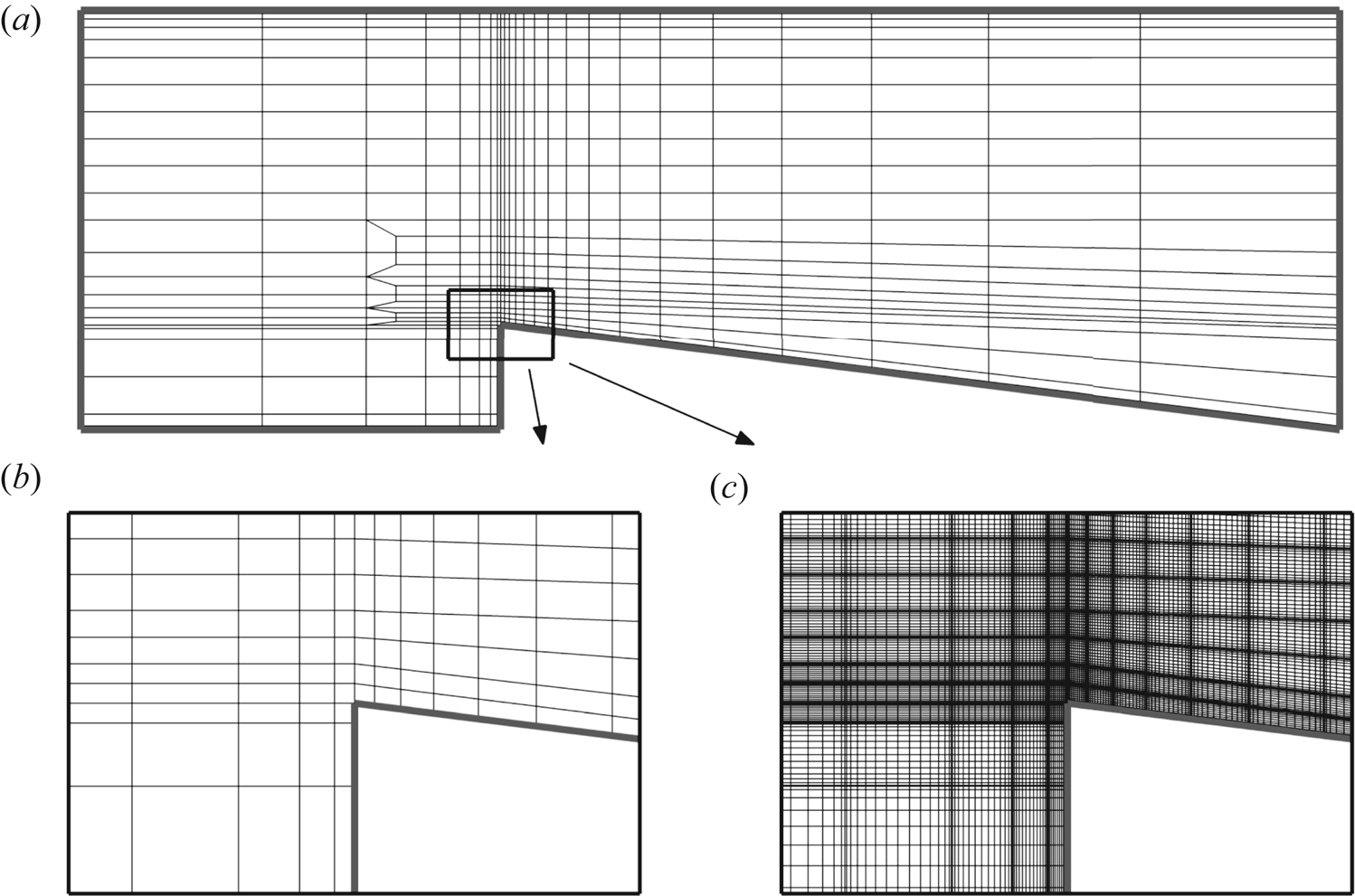
Figure 2. (a,b) Details of the  $h$-element mesh and (c) its subsequent
  $p$-refined mesh using
  $n_p=15$. Close-up views of the mesh resolution about the wedge tip are shown in (b,c). The particular geometric parameters here are
  $\beta =0.25$,
  $\gamma =2$ and
  $\tan (\phi )=0.125$. (b) Spectral elements, (c)
  $n_p=15$ quadrature points.
Table 1. Convergence of solution with increasing order of element polynomial ( $n_p$) for
  $\beta =0.25$,
  $\gamma =2$,
  $\tan (\phi )=0.125$ and
  $Re=400$. Quantities shown are the converged
  $\mathscr {L}^2$, friction factor
  $f$ of the steady base flow, percentage difference between the computed and target flow rate,
  $Q_{{diff}}$, growth rate
  $\sigma$ of the leading eigenmode at
  $k=1$ and optimal energy growth
  $G(\tau =1)$ at
  $k=0$.

For validating the computed energy growth, the computed optimal mode for  $Re=400$ at
  $\tau =5.5$ was used as the initial condition, and linearly evolved to time
  $\tau$ using (2.4)–(2.5). The energy of the evolved mode was then normalised by its initial energy and subsequently compared against the gain from the transient growth analysis:
  $G(\tau =5.5)=34.33102$. The energy ratio was found to be
 \begin{equation} \frac{K(5.5)}{K(0)}=\frac{0.00368}{0.00011}=34.32694, \end{equation}
demonstrating a relative error of less than  $0.1\,\%$ between
  $G(\tau )$ and the computationally evolved energy ratio, thus validating the accuracy of the transient growth analysis implementation.
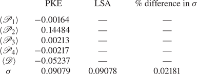
For validating the energetics analysis, the computed individual components of (2.12) are summed, yielding an estimate of the growth rate that may be compared with that computed from the linear stability analysis. These are shown in table 2 for  $\beta =0.25$ and
  $Re=400$. The relative error of growth rate from the energetics analysis is within
  $0.05\,\%$ of that computed from linear stability analysis.
Table 2. Contribution of production and dissipation terms in (2.12) to the growth rate of the leading eigenmode and its comparison with the growth rate obtained from linear stability analysis (LSA) for  $\beta =0.25$,
  $\gamma =2$,
  $\tan (\phi )=0.125$ at
  $Re=400$.
4. Two-dimensional flow
4.1. Flow regimes
Inspection of the computed 2-D flow solutions reveals that the flows may be classified into five regimes, as shown in figure 3. Regime-1 (figure 3a), occurring at low  $Re$, is characterised by a single recirculation region that develops in front of the wedge. The flow otherwise remains attached to the channel walls. The appearance of a recirculation region at a sharp concave corner is a ubiquitous feature of low Reynolds number flows (Taneda Reference Taneda1979). This is similar to the low
  $Re$ flow over a FFS in which a primary recirculation region appears in front of the step (Mei & Plotkin Reference Mei and Plotkin1986; Stüer et al. Reference Stüer, Gyr and Kinzelbach1999). With an increase in
  $Re$, an adverse pressure gradient compels the flow to separate from the wedge taper, subsequently reattaching to the bottom wall in the gap before the next wedge. This creates another recirculation region extending from the tapered surface of the current wedge to the gap between the current and the subsequent wedge (regime-2, figure 3b), unlike the flow over a FFS where a secondary recirculation region forms immediately after the step. In regime-3 (figure 3d), the recirculation region identified in regime-2 merges with the recirculation region in front of the next wedge, forming a single recirculation region extending from the slanted wedge surface of the current wedge to the front of the next wedge. For higher blockage ratios of
  $\beta \gtrsim 0.5$, an additional steady secondary recirculation region is also observed immediately downstream of the wedge tip in regime-2 and regime-3 (figure 3c). Further increasing
  $Re$ produces an unsteady flow. In unsteady regime-4 (instantaneous snapshot in figure 3e), the steady recirculation region identified in regime-3 begins to shed, introducing vortices which sweep over the bottom wall, whereas the flow remains attached on the top wall of the channel. No vortex shedding from the wedge tip is observed in this regime. The last regime encountered, regime-5 (instantaneous snapshot in figure 3f) is characterised by vortex shedding occurring at the wedge tip along with entrainment of boundary layer vorticity into the bulk.

Figure 3. (a–d) Two-dimensional steady flow regimes 1–3 and (e–f) unsteady regimes 4–5. The streamlines are shown in all cases, while an instantaneous snapshot of spanwise vorticity contours is included in the unsteady cases;  $\gamma =2$,
  $\tan (\phi )=0.125$ for all cases. Contours of spanwise vorticity are shown in the linear scale at 20 equispaced levels. (a) Regime-1,
  $\beta =0.25$,
  $Re=100$. (b) Regime-2,
  $\beta =0.25$,
  $Re=175$. (c) Regime-2,
  $\beta =0.65$,
  $Re=75$. (d) Regime-3,
  $\beta =0.25$,
  $Re=200$. (e) Regime-4,
  $\beta =0.25$,
  $Re=450$. ( f) Regime-5,
  $\beta =0.25$,
  $Re=500$.
The regime maps for a range of  $\beta$,
  $\gamma$ and
  $\phi$ are plotted in figure 4. The Reynolds number for the onset of each regime is termed
  $Re_{Ri}$, where
  $i=2\unicode{x2013}5$ denotes the regime of the flow observed at
  $Re >Re_{Ri}$;
  $Re_{R5} =Re_{cr,{2D}}$ is the approximate critical Reynolds number for the onset of 2-D vortex shedding in the flow. These threshold Reynolds numbers for changes in the steady flow topology were determined visually, accurate to within
  $\Delta Re =\pm 10$. The critical
  $Re$ for onset of the unsteady regime (
 $Re_{R4}$ for some cases if it exists,
  $Re_{R5}$ otherwise) is found through LSA, and is presented in § 5.1. The value of
  $Re_{cr,{2D}}$ decreases with increasing
  $\beta$,
  $\gamma$ and
  $\phi$. With increasing
  $\beta$, the range of
  $Re$ for each regime decreases and at higher blockage ratios, vortex shedding starts after the flow passes through two steady regimes – regimes 1 and 2. Regime-4 is not observed for
  $\beta \gtrsim 0.25$. Within
  $0.3 \lesssim \beta \lesssim 0.35$ regime-2 was not identified, whereas within
  $0.5 \lesssim \beta \lesssim 0.65$ regime-3 was not observed. A similar observation was made for
  $\gamma \gtrsim 4$. In the range of wedge angles investigated, the flow passes through each of the flow regimes identified before becoming unsteady. At higher
  $\beta$ and
  $\gamma$, each threshold
  $Re$ approaches a constant value. A similar trend can be seen with increasing
  $\phi$ for
  $Re_{R4}$.

Figure 4. Regime maps as functions of  $Re$ and (a)
  $\beta$, (b)
  $\gamma$ and (c)
  $\phi$. The fixed geometric parameters are as indicated in (a–c). The threshold Reynolds numbers for onset of each 2-D flow regime are shown in figure 3 and the 3-D instability thresholds are given by
  $Re_{R2}$,
  $Re_{R3}$,
  $Re_{R4}$,
  $Re_{R5}$ and
  $Re_{cr,3{D}}$; (a)
  $\gamma =2$,
  $\tan (\phi )=0.125$, (b)
  $\beta =0.25$,
  $\tan (\phi )=0.125$, (c)
  $\beta =0.25$,
  $\gamma =2$.
4.2. Steady separation and reattachment
To further characterise the steady 2-D flow, the behaviour of different recirculation regions in the flow is elucidated by the migration of their separation and reattachment points along the bottom wall for various blockage ratios in figure 5. The recirculation regions are places of accumulation of fluid which does not interact with the bulk flow. From a heat transfer perspective, these are regions where high temperatures may develop and, lacking convective transport and mixing, might lead to structural failure. A diagram illustrating the location of the recirculation zones and nomenclature of the separation and reattachment points is illustrated in figure 5(a). The recirculation region that forms in front of the wedge (denoted as  $1$) have separation and reattachment points
  $x_{s1}$ and
  $y_{r1}$, respectively. An increase in
  $x_{s1}$ denotes its migration to the right whereas an increase in
  $y_{r1}$ shows its movement upward on the vertical wall. For the recirculation region denoted as
  $3$, closed and open circles respectively are used to denote the separation (
 $x_{s3}$) on the tapered wall and the corresponding reattachment (
 $x_{r3}$) on the bottom wall between the current and the subsequent wedge. An increase in either of these values denotes a shift to the right. For
  $\beta \geq 0.5$, an additional recirculation region-2 appears with separation starting at the wedge tip and reattaching on the tapered wall (
 $x_{r2}$), represented by open triangle symbols. An increase in
  $x_{r2}$ shows its movement to the right, away from the wedge tip.

Figure 5. (a) A sketch showing the location of three identified recirculation zones and nomenclature of the separation (closed symbols) and reattachment points (open symbols) along with plots showing their dependence on  $Re$ and
  $\beta$ and variation along bottom (b) horizontal and slanted wall and (c) vertical wall. Horizontal dashed lines in (b,c) are used to represent the deviation from an existing trend due to the formation of a new recirculation region or merging of two existing recirculation regions for
  $\beta =0.25$,
  $\gamma =2$ and
  $\tan (\phi )=0.125$.
The trendlines showing the growth of different recirculation regions are explained for  $\beta =0.25$. The growth of recirculation region-1 is shown as a decrease in
  $x_{s1}$ and increase in
  $y_{r1}$ with
  $Re$. Deviation from this trend is observed when recirculation region-3 forms further downstream (represented by the first dashed line from the bottom in figure 5b,c). Further, the growth of recirculation region-3 with
  $Re$ is shown as an increase in
  $x_{r3}$ and an approximately linear decrease in
  $x_{s3}$. A deviation in the trend of
  $x_{s3}$ and
  $y_{r1}$ is observed when recirculation regions 1 and 3 merge, shown by the second dashed line from the bottom in figure 5. A similar trend is observed for all blockage ratios (figure 5b,c), and pitch and wedge angle variations (not shown). This behaviour was also found for flows past a BFS (Erturk Reference Erturk2008), FFS (Marino & Luchini Reference Marino and Luchini2009) and in a 180 degree bend (Sapardi et al. Reference Sapardi, Hussam, Pothérat and Sheard2017).
5. Linear stability
LSA has been used in various confined flow set-ups to identify the bifurcation in the solution branch, such as the steady 3-D bifurcation in flow over a BFS (Barkley et al. Reference Barkley, Gomes and Henderson2002; Marquet et al. Reference Marquet, Sipp, Chomaz and Jacquin2008; Lanzerstorfer & Kuhlmann Reference Lanzerstorfer and Kuhlmann2012a), the stability boundary of flow over a FFS (Lanzerstorfer & Kuhlmann Reference Lanzerstorfer and Kuhlmann2012b) and flows in a 180 degree bend (Sapardi et al. Reference Sapardi, Hussam, Pothérat and Sheard2017). This section investigates the linear stability of the steady 2-D flows reported earlier for a range of  $\beta$ and
  $\gamma$ values. The stability of the flow to 2-D perturbations is first discussed. Thereafter, the critical parameters, underlying eigenmodes and the mechanism responsible for the 3-D bifurcation are elucidated.
5.1. Two-dimensional instability
The 2-D stability of the flow is investigated in this section for a range of blockage ratios and pitch values by performing a LSA on its steady-state solutions. The resulting growth rates over a range of  $Re$ for a few
  $\beta$ and
  $\gamma$ combinations are shown in figure 6.

Figure 6. Plots of growth rate ( $\sigma$) against
  $Re$. Real and complex eigenvalues are denoted by filled and open symbols, respectively. Triangle, square and circle symbols represent modes M1, M2 and M3, respectively. All cases here have a wedge angle of
  $\tan (\phi )=0.125$; (a)
  $\beta =0.25$,
  $\gamma =2$, (b)
  $\beta =0.8$,
  $\gamma =2$, (c)
  $\beta =0.25$,
  $\gamma =1$, (d)
  $\beta =0.25$,
  $\gamma =8$.
Over almost the entire range of Reynolds numbers that produce steady flow solutions, the leading eigenmode has a real eigenvalue that remains stubbornly stable. This is labelled as the M1 mode here. As the unsteady Reynolds number regime is approached, evidence of a subdominant complex eigenmode is detected (labelled as M2 here). Using the BoostConv algorithm of Citro et al. (Reference Citro, Luchini, Giannetti and Auteri2017) steady-state solutions at higher Reynolds numbers are acquired, and analysis of these base flows reveals that this complex M2 mode rapidly overtakes the M1 mode, before becoming unstable at Reynolds numbers consistent with the appearance of unsteady flow, as described in § 4.1. The perturbation fields of the complex eigenmode (M2) responsible for the onset of 2-D unsteadiness is shown in figure 7. The eigenmode appears as a wave extending over the flow domain destabilising the shear layers on the bottom and top walls of the channel. By contrast, these oscillatory structures are absent from the M1 eigenmodes, which instead exhibits elongated streamwise structures extending the length of the domain. Since the streamwise-periodic boundary conditions imposed on this system permit only an integer number of oscillatory waves within the domain, it is possible that disturbances featuring a non-integer number of waves over any one wedge unit could lead to a slightly lower critical Reynolds number. This may explain the decrease in  $Re_{cr, {2D}}$ observed in the flow with increasing
  $\gamma$ for every fixed value of
  $\beta$. Beyond a certain
  $\gamma$ where a sufficiently wide bands of streamwise oscillation wavelengths are available,
  $Re_{cr, {2D}}$ does not vary significantly with an increase in
  $\gamma$ (figure 4b).

Figure 7. Contours of the real part of  $\hat {\omega }_{z}$ overlaid with the line contours of the real part of
  $\hat {v}$ for modes (a–d) M2 and (e, f) M3. Base flow streamlines are also shown for reference. All cases here have a wedge angle of
  $\tan (\phi )=0.125$. Contours of
  $\hat{\omega}_{z}$ are shown in the linear scale at 20 equidistant levels, while line contours of
  $\hat {v}$ are shown at 8 equidistant levels with solid and dashed lines representing positive and negative values, respectively, between
  $-$0.004 and 0.004 for (a–d, f) and between
  $-$0.002 and 0.002 for (e); (a)
  $\beta =0.25$,
  $\gamma =2$,
  $Re=450$ (M2), (b)
  $\beta =0.8$,
  $\gamma =2$,
  $Re=85$ (M2), (c)
  $\beta =0.25$,
  $\gamma =8$,
  $Re=300$ (M2), (d)
  $\beta =0.5$,
  $\gamma =16$,
  $Re=125$ (M2), (e)
  $\beta =0.25$,
  $\gamma =8$,
  $Re=300$ (M3), ( f)
  $\beta =0.5$,
  $\gamma =16$,
  $Re=125$ (M3).
To verify the findings from LSA, the steady-state solutions obtained at a Reynolds number slightly beyond  $Re_{cr,\mathrm{2D}}$ using the BoostConv algorithm are naturally evolved, and the underlying disturbance structure is monitored. It is observed that the underlying disturbance structure matches with the dominant mode (M2) obtained from LSA at longer times. Snapshots of the disturbance field at a few time instances are shown in figure 8 for
  $\beta =0.25$,
  $\gamma =2$ at
  $Re=480$ as an example. Additionally, the frequency of oscillation (
 $f_{{linear}}$) obtained from linear evolution of the unstable mode M2 (
 $f_{{linear}}=0.26$ for
  $\beta =0.25$,
  $\gamma =2$,
  $Re=480$ and
  $f_{{linear}}=0.253$ for
  $\beta =0.5$,
  $\gamma =2$,
  $Re=130$) is found to match closely with the frequency of oscillation (
 $f$) of the unsteady 2-D flow (
 $f=0.261$ for
  $\beta =0.25$,
  $\gamma =2$,
  $Re=480$ and
  $f=0.251$ for
  $\beta =0.5$,
  $\gamma =2$,
  $Re=130$), thereby supporting our finding that the onset of 2-D unsteadiness is due to the linear instability mode M2.

Figure 8. Evolution of spanwise vorticity field ( $\hat {\omega }_{z}$) of the underlying disturbance structure on naturally evolving the flow from the steady-state solution for
  $\beta =0.25$,
  $\gamma =2$,
  $\tan (\phi )=0.125$ at
  $Re=480$. The line contours of spanwise vorticity of the corresponding linear instability mode (M2) is shown at
  $t=254.2$. Contours of
  $\hat {\omega }_{z}$ of the disturbance field are shown in the linear scale at 20 equispaced levels between
  $-0.05$ (blue) to 0.05 (red), whereas the line contours of
  $\hat {\omega }_{z}$ for M2 are spaced at 10 equispaced levels in the same range with solid and dashed lines representing positive and negative values, respectively; (a)
  $t=150$, (b)
  $t=200$, (c)
  $t=250$, (d)
  $t=252$, (e)
  $t=253.6$, ( f)
  $t=254.2$.
5.2. Three-dimensional instability – growth rate and marginal stability
The stability of the steady flow to small 3-D perturbations is investigated in this section. The growth rates of the leading eigenmode are shown in figure 9 as functions of  $Re$ and spanwise wavenumber
  $k$ for selected
  $\beta$ and
  $\gamma$ combinations. The primary instability of the steady flow occurs through a stationary 3-D eigenmode (having a real eigenvalue) for all
  $\beta$ and
  $\gamma$ investigated in this study. The
  $Re$ and
  $k$ at which the maximum growth rate of the perturbation is zero are the critical Reynolds number (
 $Re_{cr, 3{D}}$) and wavenumber (
 $k_{cr}$).

Figure 9. Plots of the growth rate ( $\sigma$) of the leading eigenmode against spanwise wavenumber
  $k$ for different
  $Re$. The stability analysis was conducted for wavenumbers up to
  $k=50$, but only a small range of interest is shown here for clarity, the remaining modes always decayed monotonically with increasing wavenumber; (a)
  $\beta =0.25$,
  $\gamma =2$, (b)
  $\beta =0.8$,
  $\gamma =2$, (c)
  $\beta =0.25$,
  $\gamma =1$, (d)
  $\beta =0.25$,
  $\gamma =8$.
Inspection of the eigenvalue spectra for  $|(Re-Re_{cr, 3{D}})/Re_{cr, 3{D}}| \lesssim 0.035$ for different cases indicates a single dominant mode to be responsible for the bifurcation. In figure 10 the full eigenvalue spectrum near
  $Re_{cr, 3{D}}$ is shown for selected cases. With increasing
  $\gamma$ at a fixed blockage ratio the number of subdominant complex eigenvalues (all stable) appear to increase and are spread across the complex plane. An increase in
  $\beta$ at a fixed
  $\gamma$ shows complex subdominant eigenvalues (all stable) with only a single real eigenvalue which corresponds to the dominant eigenmode. The first subdominant mode also appears to move closer to the neutral curve with an increase in
  $\beta$ and
  $\gamma$. The dominant modes for different geometric parameter combinations are shown in figure 13 and the subdominant complex mode for
  $\beta =0.8$,
  $\gamma =2$ is shown in figure 10(e) as an example. They appear as counter-rotating streamwise vorticity structures concentrated near the wedge tip along with other pairs near the top and bottom walls seen downstream, which appear as chevron structures in the 2-D plane (not shown).

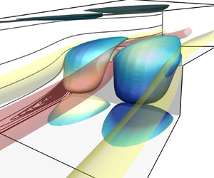
Figure 10. Eigenvalue spectra near the critical Reynolds number ( $Re_{cr,{3D}}$). The leading and first subdominant eigenvalues are indicated as (i) and (ii). Closed and open symbols denote real and complex eigenvalues, respectively. (e) Positive (blue) and negative (yellow) iso-surfaces of streamwise vorticity (
 $\hat{\omega}_{x}$) of the first subdominant eigenmode of (d), while the leading modes labelled (i) are shown in figure 13. The wedge angle
  $\tan (\phi )=0.125$ for all cases; (a)
  $\beta =0.25$,
  $\gamma =2$,
  $Re=90$, (b)
  $\beta =0.25$,
  $\gamma =8$,
  $Re=150$, (c)
  $\beta =0.5$,
  $\gamma =2$,
  $Re=60$, (d)
  $\beta =0.8$,
  $\gamma =2$,
  $Re=60$.
Marginal stability curves for selected blockage ratios and pitch values are shown in figure 11. The flow is linearly unstable at given wavenumbers to the right of these curves and stable to the left. With increasing blockage ratio, the curves shift to lower  $Re$ irrespective of the pitch and the unstable wavenumber range grows wider, indicating that higher blockages are more destabilising for the flow. At any fixed blockage ratio, decreasing
  $\gamma$ causes the flow to become more unstable, which is observed as a shift in the neutral curves to the left. This is because the effect of the wedge on the flow becomes greater with increasing constriction and decreasing distance between the wedges.

Figure 11. Neutral stability curves of the flow for different  $\beta$ and
  $\gamma$. In (c) solid curves correspond to
  $\gamma =8$ and dashed curves to
  $\gamma =16$. All the cases have a wedge angle of
  $\tan (\phi )=0.125$; (a)
  $\gamma = 2$, (b)
  $\beta =0.25$, (c)
  $\gamma = 8, 16$, (d)
  $\beta =0.8$.
In figure 4(a,b),  $Re_{cr, 3{D}}$ is overlaid on the regime maps of the 2-D base flows as functions of
  $\beta$ and
  $\gamma$. For all
  $\gamma$ investigated here and for
  $\beta \lesssim 0.5$,
  $Re_{cr, 3{D}}$ is within regime-1, where only a single recirculation region exists upstream of the wedge. For cases with
  $\beta \gtrsim 0.5$, onset of three-dimensionality occurs within regime-2 when another recirculation region is formed immediately after the wedge tip.
The resemblance of the wedge geometry to a FFS motivates a rescaling of  $Re_{cr, 3{D}}$ and
  $k_{cr}$ by constriction gap height (
 $2L-h_w$), consistent with the length scale based on the FFS downstream channel height used in Lanzerstorfer & Kuhlmann (Reference Lanzerstorfer and Kuhlmann2012b). The rescaled values are denoted as
  $Re_{cr,\beta }=2Re_{cr,3{D}}$(
 $1-\beta$) and
  $k_{cr,\beta }=2k_{cr}$(
 $1-\beta$). Similarly, to assess their variation with
  $\gamma$, they are rescaled based on the gap length
  $l_p$, i.e.
  $Re_{cr,\gamma }=\gamma Re_{cr,3{D}}$ and
  $k_{cr,\gamma }=\gamma k_{cr}$. The variation of these modified critical Reynolds number and wavenumber with
  $\beta$ at a fixed pitch of
  $\gamma =2$ and
  $\gamma =16$, as well as their variation with
  $\gamma$ at a fixed blockage ratio of
  $\beta =0.25$ and
  $\beta =0.8$, are shown in figure 12. Both
  $Re_{cr,\beta }$,
  $k_{cr,\beta }$ and
  $Re_{cr,\gamma }$,
  $k_{cr,\gamma }$ show a monotonic decrease with increasing
  $\beta$ and decreasing
  $\gamma$, irrespective of the fixed parameter. From figures 11 and 12 it can be observed that the influence of
  $\beta$ on the stability limit is greater at a larger pitch, whereas the influence of
  $\gamma$ is more pronounced at smaller values of
  $\beta$. On the other hand, the variation of critical wavenumber is almost negligible when the fixed parameter is changed.

Figure 12. Dependence of  $Re_{cr,\beta }$ and
  $k_{cr,\beta }$ on
  $\beta$ at (a)
  $\gamma =2$ and (c)
  $\gamma =16$, and
  $Re_{cr,\gamma }$ and
  $k_{cr,\gamma }$ on
  $\gamma$ at (b)
  $\beta =0.25$ and (d)
  $\beta =0.8$. All the cases have a wedge angle of
  $\tan (\phi )=0.125$. Filled circle and left triangle symbols in red in (b,d) are the corresponding
  $Re_{cr,\gamma }$ and
  $k_{cr,\gamma }$ values for a double-wedge case.
Dependence of  $Re_{cr,\beta }$ and
  $k_{cr,\beta }$ on blockage ratio is qualitatively similar to those in a FFS set-up (Lanzerstorfer & Kuhlmann Reference Lanzerstorfer and Kuhlmann2012b) in which the blockage ratio was termed the constriction ratio. For
  $\beta =0.25$ and
  $\beta =0.5$ at
  $\gamma =2$ (
 $\gamma =16$) the critical wavelength of the leading eigenmode
  $\lambda _{cr}$ for the present flow domain are
  $6.9h_w$ (
 $7.85h_w$) and
  $3.2h_w$ (
 $3.31h_w$), respectively, which fall between the corresponding
  $\lambda _{cr}$ for the FFS set-up,
  $3h_s$ and
  $1.8h_s$ (Stüer et al. Reference Stüer, Gyr and Kinzelbach1999; Lanzerstorfer & Kuhlmann Reference Lanzerstorfer and Kuhlmann2012b) and BFS set-up,
  $10h_s$ and
  $7.16h_s$ (Blackburn et al. Reference Blackburn, Barkley and Sherwin2008a; Lanzerstorfer & Kuhlmann Reference Lanzerstorfer and Kuhlmann2012a). The value of
  $Re_{cr, 3{D}}$ in the present system is much lower than in those geometries. The disturbances from a leading wedge carry on to subsequent wedges in the present set-up due to the streamwise-periodic domain, therefore the flow is pre-disturbed at the inlet of a subsequent wedge, altering the stability characteristics. Figure 4(b) demonstrates that
  $Re_{cr, 3{D}}$ increases with increasing pitch. This is likely because a larger pitch effectively allows the disturbances to decay more before re-entering the domain to interact with a subsequent wedge, thereby increasing the stability. The increasing value of
  $Re_{cr, 3{D}}$ with increasing
  $\gamma$ and decreasing
  $\beta$ can also be attributed to the fact that those changes direct the present set-up towards a plane channel flow. These trends demonstrate that the periodic arrangement is favourable for promoting instability; as the distance between adjacent wedges increases, the flow becomes more stable.
5.3. Three-dimensional eigenmodes and instability mechanism
In this section the 3-D eigenmodes and the underlying mechanism which destabilises the steady base flow are discussed. Examples of these modes, visualised through their streamwise vorticity  $\hat {\omega }_{x}$ and velocities
  $\hat {\boldsymbol {u}}$, are shown in figure 13. Instability manifests as a pair of counter-rotating streamwise vortices about the wedge for all blockage ratios. For
  $\beta \gtrsim 0.5$, as the influence of the top wall becomes greater, an additional pair of streamwise vortices emerges near the top wall above the wedge. For
  $\beta =0.8$ and
  $\beta =0.8$, an additional pair of streamwise perturbation velocity streaks also forms after the constriction near the top wall. The region of non-zero
  $\hat {w}$ of the eigenmode extends from the primary recirculation region over to the tip of the wedge and appears as counter-rotating spanwise rolls concentrated inside and outside the primary recirculation region (figure 14). For
  $\beta \gtrsim 0.5$, when a recirculation region is formed downstream of the wedge tip, the region of non-zero
  $\hat {w}$ extends over the separating streamline of that recirculation region, appearing as counter-rotating spanwise rolls located outside the secondary recirculation region (figure 14). The structure of the eigenmodes appears to be unaffected by
  $\gamma$ at the blockage ratios investigated, an example of which is shown in figure 13(j). The eigenmodes of the FFS (Lanzerstorfer & Kuhlmann Reference Lanzerstorfer and Kuhlmann2012b) and BFS set-ups for lower expansion ratios (Barkley et al. Reference Barkley, Gomes and Henderson2002; Lanzerstorfer & Kuhlmann Reference Lanzerstorfer and Kuhlmann2012a) appear as spanwise rolls concentrated entirely inside the recirculation region formed after the step. The eigenmodes for the current set-up shows resemblance to those modes as, elucidated in figure 14, in which
  $\hat {w}$ contours in the middle of the primary and secondary recirculation regions and a subsequent position further downstream in the flow domain are shown.

Figure 13. (a,d,g,j,m) Positive (blue) and negative (yellow) iso-surfaces of streamwise vorticity  $\hat {\omega }_{x}$ of the leading eigenmodes, (b,e,h,k,n) spanwise velocity (
 $\hat {w}$) contours overlaid with base flow streamlines and (c, f,i,l,o) positive and negative iso-contours of streamwise (
 $\hat {u}$) (represented as translucent surfaces) and transverse (
 $\hat {v}$) velocities (represented as opaque surfaces) of the leading mode. All the cases have a wedge angle of
  $\tan (\phi )=0.125$. The
  $\hat {w}$ contours are shown in the linear scale at 20 equispaced levels between
  $-0.001$ (blue) and 0.001 (red). (p–r) Show the corresponding quantities as in (a–c) for a double-wedge case.

Figure 14. Contours of  $\hat {w}$ appearing as counter-rotating rolls at
  $x=1.0$ (middle of the primary recirculation region),
  $x=2.3$ (middle of the secondary recirculation region) and
  $x=6.0$ along with the base flow streamline for
  $\beta =0.5$,
  $\gamma =2$,
  $\tan (\phi )=0.125$ at
  $Re=100$. The
  $\hat {w}$ levels are the same as in figure 13.
The imposition of streamwise periodicity over a single wedge in the present study raises the question as to whether this constraint excludes modes or flow features that would span multiple wedges. To test this, simulations have been performed in domains containing two successive wedges. Two distinct blockage ratios  $\beta =0.25$ and
  $\beta =0.8$ were considered, both having
  $\gamma =2$ and
  $\tan (\phi )=0.125$. The critical Reynolds number and wavenumber for the double-wedge cases are found to match well with the corresponding values found using a single wedge. These are shown in figure 12(b,d). The global modes for the double-wedge cases also closely resemble the modes predicted using a single wedge, and are shown in figure 13(m–o) for a single case. These results provide evidence in support of the periodic single-wedge results reported herein as being representative of multi-wedge duct flows.
Barkley et al. (Reference Barkley, Gomes and Henderson2002) found the region of maximum net outward angular momentum decrease, based on a modified inviscid centrifugal instability criterion given by Rayleigh (Bayly Reference Bayly1988), along the closed streamline of the recirculation region matching regions of peak three-dimensionality (spanwise velocity component) in a BFS set-up. Hence, they argued that centrifugal instability of the primary recirculation region was responsible for destabilising the flow. The associated eigenmode appeared as two counter-rotating spanwise velocity components concentrated entirely inside the recirculation region. This, however, is not the case for the periodic wedge set-up here, as the spanwise velocity component does not peak along the closed streamlines of the recirculation region. Another common vortex instability mechanism, elliptical instability, arises in strained vortices where perturbations grow strongly in the core of the strained vortex in the direction of the principal strain (Bayly, Orszag & Herbert Reference Bayly, Orszag and Herbert1988; Thompson, Leweke & Williamson Reference Thompson, Leweke and Williamson2001; Lanzerstorfer & Kuhlmann Reference Lanzerstorfer and Kuhlmann2012a). No evidence of elliptic instability was detected in the eigenmodes in the present study.
For flow over a BFS, Ghia et al. (Reference Ghia, Osswald and Ghia1989) argued that instability manifests as Taylor–Görtler vortices in the bulk flow, forming along curved streamlines induced by the strong recirculation regions on the top and bottom walls. They argue that, until the appearance of the secondary recirculation region on the top wall, the dividing streamline at the point of separation of the primary recirculation region remains almost parallel to the flow direction and has a convex curvature further downstream and hence the flow remains stable. Destabilisation of the flow begins with the formation of a secondary recirculation region on the top wall. Taylor–Görtler vortices appear as streamwise counter-rotating vortices. The formation of these vortices occurs in flow over concave curvature and also when the dividing streamline of the recirculation region separates at an angle to the main flow direction (Smith Reference Smith1955; Drazin & Reid Reference Drazin and Reid2004). Unlike the flow topology in Ghia et al. (Reference Ghia, Osswald and Ghia1989), in the present set-up a secondary recirculation region on the top wall is absent in the steady base flow where instability occurs. The separating streamline of the recirculation region formed at the face of the wedge for higher blockage ratio has a concave curvature and the modes appear as counter-rotating streamwise vortices over this recirculation region. Since these modes persists even for lower blockage ratios, where the separating streamline is almost parallel to the flow direction, this mechanism might not be responsible for the onset of three-dimensionality in the flow. An assessment of the PKE budget in § 5.4 will reinforce this point.
Formation of the streamwise velocity ( $\hat {u}$) streaks extending through the flow domain, as shown in figure 13(c, f,i,l), is characteristic of the lift-up mechanism (Landahl Reference Landahl1975) where a small transverse velocity component moves the fluid to a high-velocity region leading to the formation of streaks. These streaks match with the experimental observation in a FFS set-up (Stüer et al. Reference Stüer, Gyr and Kinzelbach1999). For FFS (Lanzerstorfer & Kuhlmann Reference Lanzerstorfer and Kuhlmann2012b) and BFS set-ups at lower expansion ratio (Lanzerstorfer & Kuhlmann Reference Lanzerstorfer and Kuhlmann2012a), this mechanism was found to be responsible for the instability. As a first step to check whether the lift-up mechanism underpins the instability here, the relative proportion of individual perturbation velocity components to their norms is quantified. In figure 15(a–d), ratios of the integral of the different velocity components of the leading eigenmode are plotted along the streamwise direction (
 $x$) for blockage ratios ranging from
  $\beta =0.25$ to
  $\beta =0.8$ at
  $\gamma =2$, along with the contours of absolute velocity of the leading eigenmode for each case. The plotted quantities are ratios of the following integrals:
 \begin{equation} I_{i}=\int_{y_{x,b}}^{2L} |\hat{u}_{i}| \, \mathrm{d} y, \quad I_{{total}} =\int_{y_{x,b}}^{2L} |\hat{\boldsymbol{u}}| \, \mathrm{d} y, \end{equation}
where  $y_{x,b}$ is the
  $y$ coordinate of the bottom wall at the corresponding
  $x$-position and indices
  $i=1-3$ correspond to the velocity components
  $\hat {u}$,
  $\hat {v}$ and
  $\hat {w}$, respectively.

Figure 15. Variation of  $I_1/I_{{total}}$ (dashed line),
  $I_2/I_{{total}}$ (dash-dotted line) and
  $I_3/I_{{total}}$ (thin solid line) with streamwise coordinate
  $x$. Contours of absolute velocity (
 $|\hat {\boldsymbol {u}}|$) of the leading mode in the flow domain are also shown in the linear scale at 10 equispaced levels. The wedge angle for all cases here is
  $\tan (\phi )=0.125$; (a)
  $\beta =0.25$,
  $\gamma =2$,
  $Re=400$, (b)
  $\beta =0.5$,
  $\gamma =2$,
  $Re=100$, (c)
  $\beta =0.65$,
  $\gamma =2$,
  $Re=75$, (d)
  $\beta =0.8$,
  $\gamma =2$,
  $Re=75$, (e)
  $\beta =0.5$,
  $\gamma =8$,
  $Re=70$, ( f)
  $\beta =0.5$,
  $\gamma =16$,
  $Re=100$.
For  $\beta =0.25$ and
  $\gamma =2$,
  $I_2$ and
  $I_3$ are an order of magnitude smaller than
  $I_1$ and are limited to the free shear layers formed in front of the wedge near the reattachment point
  $y_{r1}$ (figure 15a). With increasing
  $\beta$,
  $I_3$ increases at the expense of
  $I_1$ near the vertical wedge wall, and for
  $\beta \gtrsim 0.65$ (figure 15c,d),
  $I_3$ exceeds
  $I_1$ locally before relaxing back to its pre-disturbed levels, indicative of the lift-up mechanism. Similar observations were made for other
  $\beta$ and
  $\gamma$ combinations. Flows in a set-up with
  $\beta =0.5$ when varying
  $\gamma$ (figure 15e–f) are shown as examples to demonstrate that the contributions
  $I_i$ remain similar when varying
  $\gamma$ as they did with
  $\beta$ variation, indicating that the instability mechanism is not influenced by changes in
  $\gamma$.
5.4. Energetics of the 3-D instability modes
This section utilises the energy analysis described in § 2.4 to investigate the factors that contribute to perturbation growth. Local changes in the base flow and its contribution to the growth rate of the leading eigenmodes are discussed. Contributions of the terms in (2.12) to the growth rate of the leading eigenmode for all the investigated cases are shown in table 3. The largest contribution (corresponding to the largest positive value) to the growth rate, and thus the instability, comes from the production term  $\langle \mathscr {P}_2 \rangle = (1/2E_{k})\int _{\varOmega } \overline {u'v'} \partial {U}/\partial y \, \mathrm {d}\varOmega$ for all cases investigated, whereas the most stabilising contribution (corresponding to the negative value having largest magnitude) comes from the dissipation term
  $\langle \mathscr {D} \rangle$. At
  $\gamma =2$, the production term
  $\langle \mathscr {P}_1 \rangle$ has a net stabilising contribution for lower blockage ratios
  $\beta =0.125$,
  $0.25$ and the highest blockage ratio investigated here
  $\beta =0.8$, whereas for intermediate blockage ratios
  $0.5 \lesssim \beta \lesssim 0.65$, their net contribution is positive, although an order of magnitude lower than the dominant production term
  $\langle \mathscr {P}_2 \rangle$. Terms
  $\langle \mathscr {P}_3 \rangle$ and
  $\langle \mathscr {P}_4 \rangle$ have net positive and negative contributions, respectively, for all cases investigated, although they are typically more than an order of magnitude smaller than the dominant production term
  $\langle \mathscr {P}_2 \rangle$. The dominance of the production term
  $\langle \mathscr {P}_2 \rangle$ for all the cases investigated shows that the mode gains energy predominantly through horizontal shear in the base flow. The streamwise velocity dominance of the perturbations in the flow domain as shown in § 5.3 along with the fact that
  $\langle \mathscr {P}_2 \rangle$ is the largest contributor to
  $\sigma$ confirms that the lift-up mechanism is responsible for the instability in the range of geometric parameters investigated.
Table 3. Contributions of volume integrated quantities of each term in (2.12) and their percentage relative contribution to the growth rate  $\sigma$ (enclosed in brackets) of the leading eigenmode for different
  $\beta$ and
  $\gamma$ at
  $Re$ as indicated. The wedge angle is
  $\tan (\phi )=0.125$ in all cases. The largest destabilising (positive terms) and stabilising (negative terms) contributions are shown in bold.
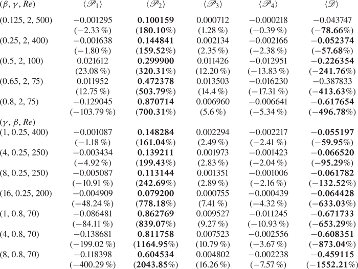
Spatial contours of the terms of (2.10), which are the integrands of (2.13)–(2.14), are shown in figure 16. These plots for different  $\beta$ and
  $\gamma$ combinations are visually similar to those already shown in figure 16. The regions in the flow domain where the streamwise and transverse velocities of the eigenmode grow due to strong streamwise and transverse velocity gradients in the base flow respectively are shown in the contours of
  $\overline {\mathscr {P}_1}$ and
  $\overline {\mathscr {P}_4}$. The streamwise velocity of the eigenmode grows predominantly in the region aft of the wedge tip (above the second recirculation region for
  $\beta \gtrsim 0.5$) and before the wedge. With increasing blockage ratio, the gain in the latter region is higher due to increasing streamwise velocity gradient in the base flow, as seen from the contours of
  $\overline {\mathscr {P}_1}$. The transverse velocity growth magnitude is highest inside the recirculation region formed before the wedge, where
  $\overline {\mathscr {P}_4}$ is stabilising (light contours in figure 16 for
  $\overline {\mathscr {P}_4}$). For higher
  $\beta$, due to the steeper transverse gradient in the constriction region above and after the wedge tip, a larger magnitude in
  $\hat {v}$ is observed in a similar region where
  $\overline {\mathscr {P}_4}$ makes a positive contribution to the growth rate (dark contours in figure 16 for
  $\overline {\mathscr {P}_4}$). The locations in the flow domain making the largest contribution to the perturbation growth rate due to strong horizontal and vertical shear in the base flow are shown in the contour plots for
  $\overline {\mathscr {P}_2}$ and
  $\overline {\mathscr {P}_3}$, respectively. Most of the dissipation
  $\bar {\mathscr {D}}$ is observed to occur about the wedge. The bottom row for each case shows the combined contributions of the terms shown (
 $\overline {\sum }$) to the growth of the leading eigenmode, superimposed by
  $\hat {w}$ line contours. The region of maximum
  $\hat {w}$ growth found in § 5.3 is where the net contribution
  $\overline {\sum }$ makes a highly stabilising contribution to the growth rate of the eigenmode, whereas the region dominated by the streamwise velocity contribution is where
  $\overline {\sum }$ makes the highest contribution to the growth rate. This confirms the statement made in § 5.3 that the Taylor–Görtler-type instability is not responsible for the formation of streamwise counter-rotating vortices.

Figure 16. Contours of terms from the spanwise-averaged PKE evolution equation (2.10) and their corresponding sum for the leading eigenmode overlaid with line contours of  $\hat {w}$. Fixed geometric parameters used are
  $\gamma =2$ and
  $\tan (\phi )=0.125$. Contours are shown in linear scale at 10 equispaced levels with the darker (lighter) shade indicating destabilising (stabilising) effect on the base flow.
6. Adjoint modes, sensitivity and endogeneity
In this section, the dynamics of the flow is explained further by computing the adjoint eigenmodes and their structural sensitivity for different geometric parameters which could also be useful from a flow control perspective. The power of adjoint analysis for flow control and sensitivity study was established for cylinder wakes by Giannetti & Luchini (Reference Giannetti and Luchini2007). Similar analysis for FFS (Marino & Luchini Reference Marino and Luchini2009) and smoothed BFS set-ups (Marquet et al. Reference Marquet, Lombardi, Chomaz, Sipp and Jacquin2009) revealed regions for placement of active and passive flow control mechanisms. The region of largest magnitude of the adjoint modes is where the flow is most receptive to initial conditions or momentum forcing which an active flow control device could exploit to produce an optimal response in terms of amplification of the instability (Hill Reference Hill1995; Akervik et al. Reference Akervik, Hœpffner, Ehrenstein and Henningson2007; Giannetti & Luchini Reference Giannetti and Luchini2007). Hill (Reference Hill1995) and later Giannetti & Luchini (Reference Giannetti and Luchini2007) have also shown that the overlap region is most sensitive to any localised feedback, which could be by the introduction of a passive structure to the flow (Strykowski & Sreenivasan Reference Strykowski and Sreenivasan1990), as it has the most impact on the eigenvalue of the linearised operator. The sensitivity field hence shows the wavemaker region or the location of the origin of the instability (Chomaz Reference Chomaz2005).
An analysis of the receptivity and sensitivity of the flow is carried out for a  $Re > Re_{cr, {3D}}$ for a range of blockage ratios and pitch values. The regions in the flow most receptive to momentum forcing is shown in the left column of figure 17. For
  $\gamma =2$, the receptive region spans the incline of the wedge until the separation point and stretches further downstream with increasing
  $\beta$. For larger
  $\gamma$, additional receptive regions form in the gap between wedges (figure 17i,k), similar to what is observed in a FFS set-up (Marino & Luchini Reference Marino and Luchini2009; Lanzerstorfer & Kuhlmann Reference Lanzerstorfer and Kuhlmann2012b). The sensitive location given by the overlap region of the adjoint and direct mode's magnitude is shown for different
  $\beta$ and
  $\gamma$ in the right column of figure 17. The wavemaker is located in the region of strong base flow shear extending downstream of the wedge tip. At
  $\gamma =2$ and with increasing blockage ratio (
 $\beta \geq 0.5$), a recirculation region forms immediately after the wedge tip causing a shift in the most sensitive region away from the wedge tip, to between the two recirculation regions on the tapered wedge surface. With increasing pitch, the sensitive locations appear to extend further downstream from the wedge tip to the gap between the wedges (figure 17j,l). These sensitive regions strongly resemble the contours of
  $\overline {\mathscr {P}_2}$ in figure 16. These are regions in the flow that are important for the placement of a passive flow control mechanism in the flow (Strykowski & Sreenivasan Reference Strykowski and Sreenivasan1990; Akervik et al. Reference Akervik, Hœpffner, Ehrenstein and Henningson2007; Giannetti & Luchini Reference Giannetti and Luchini2007; Marquet et al. Reference Marquet, Lombardi, Chomaz, Sipp and Jacquin2009).

Figure 17. Receptivity to initial condition/momentum forcing (a,c,e,g,i,k) and structural sensitivity (b,d, f,h,j,l) of the unstable 3-D eigenmodes. Contours are shown in the linear scale at 10 equispaced levels.
The endogeneity distribution and the real part of the individual contributions in (2.20) are examined to understand the local contribution to the growth rate of the destabilising eigenmode and to compare the integral values contributing to the growth rate found from the PKE analysis. The largest positive contribution to the growth rate of the global mode comes from the production due to base flow shear, whereas the largest negative contribution is from viscous dissipation of the perturbation velocity, consistent with the energetics analysis in § 5.4. However, a distinction from the PKE analysis is that there is also a destabilising contribution from convection of the perturbation by base flow velocity and the pressure forces. The convection contribution is modest, being almost an order of magnitude smaller than the production contribution. The pressure contribution should intrinsically integrate to zero, so its small finite values (being four to five orders of magnitude smaller than the production contributions) can be interpreted as an indication of the error level in the endogeneity calculations. These values are compared in table 4.
Table 4. Comparison of the contribution of volume integrated quantities of each term in (2.12) and the domain integral of the real part of individual terms in (2.20) with the growth rate  $\sigma$ of the leading eigenmode for different
  $\beta$ and
  $\gamma$ at
  $Re$ as indicated. The wedge angle is
  $\tan (\phi )=0.125$ in all cases. Positive (negative) terms have a destabilising (stabilising) contribution.
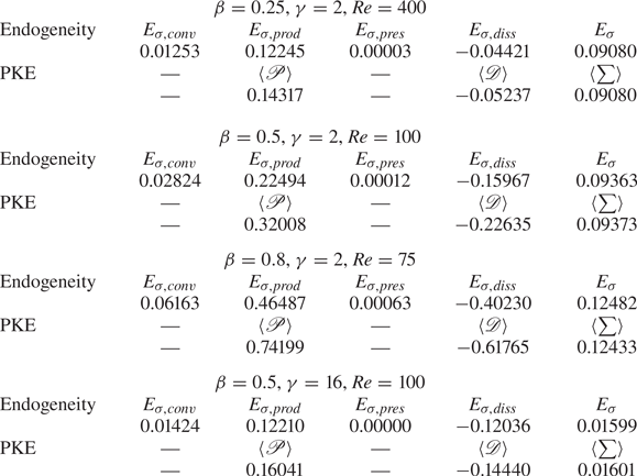
The total endogeneity field shown in figure 18(e) shows a local stabilising contribution (negative values) around the wedge tip and a destabilising contribution (positive values) to the growth rate of the global mode in regions covering approximately half the constriction height. Similar observation was also made for blockage ratios up to  $\beta =0.8$ all with
  $\gamma =2$ and
  $\beta =0.5$,
  $\gamma =8$, although the destabilising region occupied more of the constriction gap with increasing blockage ratio. The individual component contributions in figure 18(a–d) shown for
  $\beta =0.25$,
  $\gamma =2$ with
  $\tan (\phi )=0.125$, reveal that the local contribution from the perturbation pressure gradient term swamps the total endogeneity, as
  $E_{\sigma }$ closely resembles
  $E_{\sigma, {pres}}$ for this case, and does not exhibit similarity to the wavemaker region obtained from the sensitivity analysis (figure 17c,d). This contrasts with the case of 2-D instability of the circular cylinder wake, in which the local endogeneity distribution exhibited qualitative similarity to the wavemaker region found from the sensitivity studies (Marquet & Lesshafft Reference Marquet and Lesshafft2015; Paladini et al. Reference Paladini, Marquet, Sipp, Robinet and Dandois2019). However, the region contributing most strongly to the growth rate predicted from the spanwise-averaged distribution of all contributions from the PKE analysis (figure 16) resembles more closely the sum of contributions from
  $E_{\sigma,{conv}}$,
  $E_{\sigma,{prod}}$ and
  $E_{\sigma,{diss}}$, as shown in figure 18( f). In contrast, the endogeneity for a longer pitch case of
  $\gamma =16$ at
  $\beta =0.5$ (figure 19e) showed a different distribution compared with the previous case, with a weaker distribution of the pressure contribution, which also shows a different distribution from the aforementioned case. In this case, the endogeneity distribution matches with the wavemaker region predicted from an exogeneous approach (figure 17k,l) with a stronger distribution around the wedge tip for the endogeneity field. The fields showing the individual contributions for this case are shown in figure 19(a–d), with the sum of contributions from
  $E_{\sigma,{conv}}$,
  $E_{\sigma,{prod}}$ and
  $E_{\sigma,{diss}}$ shown in figure 19(e). The sudden constriction due to the presence of the wedge might be one possible reason for the local pressure gradient to contribute significantly to the growth rate for all blockage ratios with the low pitch of
  $\gamma =2$ investigated in this study. The impact of the subsequent wedge relaxes further with increasing
  $\gamma$, which may explain why the pressure term has a weaker influence on the endogeneity in the case of
  $\gamma =16$,
  $\beta =0.5$.

Figure 18. (a–d) Contribution of the real part of the individual endogeneity terms in (2.20) to the (e) endogeneity distribution and ( f) sum of the convection, production and the dissipation contributions for  $\beta =0.25$,
  $\gamma =2$ and
  $\tan (\phi )=0.125$ at
  $Re=400$. Note that
  $E=E_{\sigma }$ as the global mode has a real eigenvalue. Contours are shown in the linear scale at 20 equispaced levels; (a)
  $E_{\sigma,{conv}}$, (b)
  $E_{\sigma,{prod}}$, (c)
  $E_{\sigma,{pres}}$, (d)
  $E_{\sigma,{diss}}$, (e)
  $E_{\sigma }$, ( f)
  $E_{\sigma,{conv}}+E_{\sigma,{prod}}+ E_{\sigma,{diss}}$.

Figure 19. (a–d) Contribution of the real part of the individual endogeneity terms in (2.20) to the (e) endogeneity distribution and ( f) sum of the convection, production and the dissipation contributions for  $\beta =0.5$,
  $\gamma =16$ and
  $\tan (\phi )=0.125$ at
  $Re=100$. Note that
  $E=E_{\sigma }$ as the global mode has a real eigenvalue. Contours are shown in the linear scale at 20 equispaced levels; (a)
  $E_{\sigma,{conv}}$, (b)
  $E_{\sigma,{prod}}$, (c)
  $E_{\sigma,{pres}}$, (d)
  $E_{\sigma,{diss}}$, (e)
  $E_{\sigma }$, ( f)
  $E_{\sigma,{conv}}+E_{\sigma,{prod}}+ E_{\sigma,{diss}}$.
7. Linear transient growth
A large transient growth associated with convective instabilities has been found in the linearly stable region in similar channel flow set-ups such as BFS (Blackburn, Sherwin & Barkley Reference Blackburn, Sherwin and Barkley2008b), rounded BFS (Marquet et al. Reference Marquet, Sipp, Chomaz and Jacquin2008) and stenotic flows (Blackburn et al. Reference Blackburn, Sherwin and Barkley2008b; Griffith et al. Reference Griffith, Leweke, Thompson and Hourigan2008). Such large transient amplification of disturbances over short time scales can occur in flows due to non-modal interactions, potentially triggering a bypass transition. By contrast, the analysis to follow demonstrates that both 2-D and 3-D disturbances in the present set-up exhibit modest linear transient growth.
7.1. Optimal growth of 2-D disturbances
The 2-D optimal disturbances in the linearly stable 2-D regimes from § 5.1 are presented for various combinations of  $\beta$ and
  $\gamma$ over a range of Reynolds numbers. Optimal energy gain for a range of
  $Re$ is shown in figure 20(a) as a function of time
  $\tau$ for
  $\beta =0.25$ with
  $\gamma =2$. For
  $Re>40$, the optimal mode achieves a gain exceeding unity, reaching a maximum value
  $G_{max}$ at an optimal time
  $\tau _{opt}$, both of which increase with increasing
  $Re$. For
  $Re \gtrsim 400$, a second peak with lower gain than the first peak is observed, which is due to the interaction of the disturbance structure with the subsequent wedge and the free shear layers near the vertical wall of the wedge. Eventually, the energy in the disturbance structure monotonically decreases with increasing time horizon for all
  $Re$ in the range investigated. This is in agreement with the observation from the LSA, where the 2-D perturbations are asymptotically stable. In the contour plot in figure 20(b),
  $\log _{10}G(\tau )$ is plotted on the
  $Re-\tau$ plane. The point on the
  $Re$ axis where
  $\log _{10}G(\tau )=0$ gives a Reynolds number
  $Re_{E}$ below which all perturbations decay without any transient growth. For the case shown in figure 20(b) with
  $\beta =0.25$ and
  $\gamma =2$,
  $Re_{E} \approx 42.09$ while
  $Re_{cr, 2D} = 446$, as predicted from the stability analysis in § 5.1, the difference between these Reynolds numbers indicating the range where convective instabilities may be excited to an absolute state depending on the disturbance shape and amplitude.

Figure 20. (a) Two-dimensional optimal growth  $\log _{10}G(\tau )$ curves for
  $Re$ from
  $40$ to
  $430$. Dashed horizontal line represents the neutral line and, (b) contours of
  $\log _{10}G(\tau )$ (positive to negative shown as red to blue) plotted on
  $Re-\tau$ plane for
  $\beta =0.25$ with
  $\gamma =2$,
  $\tan (\phi )=0.125$.
The 2-D optimal modes (shown in the first panel of figure 21) are composed of narrow inclined structures of alternately sign, opposing the mean flow direction that are concentrated before the first separation point of the base flow after the wedge tip ( $x_{s3}$ in figure 5). The linear evolution of the optimal mode at
  $Re=400$ is elucidated in figure 21 and is also provided in the first video in the supplementary material available at https://doi.org/10.1017/jfm.2022.200. Over time, the disturbances are advected downstream by the base flow, and the slanted structures are slowly rotated to an upright orientation by the background shear, suggesting the energy gain in the disturbance structure is by the 2-D Orr mechanism (Orr Reference Orr1907). On interaction with the subsequent wedge, the disturbance structure also gains energy from the free shear layers about the wedge tip. This can be observed from the increased density of line contours of PKE carried by the disturbance as it impinges on the subsequent wedge (figure 21, panel corresponding to
  $\tau _{opt}$). Similar observation can be made from the energy contours corresponding to the subsequent peaks labelled as
  $T2$ and
  $T3$ and
  $T4$ in figure 22 suggesting a contribution to the energy growth of the disturbance at impingement on the wedge wall. The lower energy gain in the subsequent peaks indicates that the optimal mode gains energy predominantly through its tilting in the base flow direction (the Orr mechanism), as this feature is only present through the primary
  $E(t)/E(0)$ maximum.

Figure 21. Spanwise perturbation vorticity ( $\hat {\omega }_{z}$) contours overlaid by perturbation kinetic energy contours (black line contours) for
  $\beta =0.25$,
  $\gamma =2$ at
  $Re=400$, and its linear evolution over time. The initial condition at
  $t=0$ corresponds to the optimal mode, and the subsequent time instants of each frame correspond to the marker positions shown in figure 22(a). The dividing streamline of the base flow is shown in white. The
  $\hat {\omega }_{z}$ contours are shown in linear scale at 20 equispaced levels whereas energy iso-contours are shown at 5 equispaced levels between
  $0$ and
  $0.0006$; (a)
  $t=0$, (b)
  $t=2$, (c)
  $t=3$, (d)
  $t=\tau _{opt}=5.5$, (e)
  $t=8$, ( f)
  $t=10$, (g)
  $t=11.2$ (
 $T2$), (h)
  $t=12.7$, (i)
  $t=15.2$ (
 $T3$), (j)
  $t=16.8$ (
 $T4$), (k)
  $t=20$, (l)
  $t=37.8$.

Figure 22. Comparison of energy curve obtained by linear evolution of 2-D optimal mode for different (a)  $\gamma$ at
  $\beta =0.25$ and (b)
  $\beta$ at
  $\gamma =2$. Wedge angle
  $\tan (\phi )=0.125$ for all the cases.
The influence of  $\gamma$ and
  $\beta$ on the disturbance energy on linear evolution starting from the optimal mode is shown in figure 22. At
  $\beta =0.25$ and large
  $\gamma$, the base flow reattaches to the channel bottom wall well before the subsequent wedge (
 $x_{r3}$ in figure 5) unlike at
  $\gamma \lesssim 2$, where the recirculation region extends across the entire gap between the wedges. The energy gain from the larger extent of the free shear layer near the wedge wall at lower
  $\gamma$ could possibly be the reason for a higher optimal energy gain in those cases. The energy in successive peaks is also observed to be lower at higher
  $\gamma$ (figure 22a) since the disturbances decay much more in the gap before reaching the subsequent wedge. Contours showing the linear evolution of the optimal mode for
  $\gamma =8$ are provided in the supplementary material. At a low pitch of
  $\gamma =2$, increasing the blockage ratio also results in a lower optimal growth (shown for
  $\beta =0.5$ in figure 22b) since channel wall interactions at large blockage ratios limit the tilting of the optimal disturbances, and hence their energy gain. The linear evolution of the optimal mode for a higher blockage ratio case of
  $\beta =0.5$,
  $\gamma =2$ at
  $Re=100$ is also provided in the supplementary material.
The variation of  $G_{max}$ and
  $\tau _{opt}$ for various combinations of
  $\beta$ and
  $\gamma$ are shown in figure 23 for Reynolds numbers interpolated at
  $Re/Re_{cr,2D} = 0.85$ and
  $0.95$. In the range of parameters investigated,
  $G_{max}$ is highest in the range
  $1\lesssim \gamma \lesssim 4$ for
  $\beta =0.25$, whereas for
  $\beta =0.5$,
  $G_{max}$ decreases monotonically until
  $\gamma \approx 8$ and a slightly higher value is found at
  $\gamma =16$. The optimal time horizon (
 $\tau _{opt}$) appears to increase with
  $\gamma$ in the low range for both
  $\beta =0.25$ and
  $0.5$, and decreases slowly at higher
  $\gamma \gtrsim 8$ for
  $\beta =0.25$, whereas it appears to plateau for
  $\beta =0.5$. The largest energy gain possible (
 $G_{max}$) is consistently lower at a higher blockage ratio of
  $\beta =0.5$ than those obtained at
  $\beta =0.25$ for all
  $\gamma$ in this study due to the limited tilting of the disturbances explained earlier.

Figure 23. Variation of (a)  $G_{max}$ and (b)
  $\tau _{opt}$ with
  $\gamma$ for
  $\beta =0.25$ (filled symbols, solid line) and
  $\beta =0.5$ (open symbols, dashed line). Square symbols are interpolated at
  $Re=0.85 Re_{cr,{2D}}$ and triangle symbols at
  $Re=0.95 Re_{cr,{2D}}$.
7.2. Optimal growth of 3-D disturbances
Attention is now turned to the optimal growth of 3-D disturbances for subcritical Reynolds numbers, i.e.  $Re < Re_{cr,{3D}}$. For different Reynolds numbers, transient growth amplification factors are determined for various spanwise wavenumbers
  $k$ and time horizons
  $\tau$. For each
  $\tau$, optimal energy growth increases to maximum, before decreasing with increasing
  $k$. An iso-surface plot showing the variation of the optimal energy growth for
  $\beta =0.5$,
  $\gamma =2$ at
  $\varepsilon =Re/Re_{cr,{3D}}=0.92$ is given in figure 24(a). An optimal wavenumber
  $k_{opt}$ exists corresponding to
  $G_{max}$ for each Reynolds number.

Figure 24. (a) Variation of the optimal energy growth  $G(\tau )$ represented as functions of spanwise wavenumber (
 $k$) and time (
 $\tau$) for
  $\beta =0.5$,
  $\gamma =2$ at
  $\varepsilon =0.92$ and (b) variation of maximum optimal energy growth
  $G_{max}$ with
  $\varepsilon =Re/Re_{cr,{3D}}$. For all the cases
  $\tan (\phi )=0.125$.
To demonstrate how the maximum optimal growth over all possible spanwise wavenumbers  $G_{max}$ changes on approaching
  $Re_{cr,{3D}}$ and when varying blockage ratio and pitch, three different geometric parameter cases are considered (figure 24b). At a lower blockage ratio of
  $\beta =0.25$ with
  $\gamma =2$, and
  $\gamma=8$, the maximum optimal growth varies exponentially as
  $G_{max} \sim e^{2.76 \varepsilon}$ and
  $G_{max} \sim e^{3.09 \varepsilon}$, respectively. At a higher blockage ratio of
  $\beta =0.8$ at
  $\gamma =2$, an exponential increase in the maximum optimal growth,
 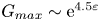 $G_{max} \sim {\rm e}^{4.5\varepsilon }$ was found, although the maximum growth remained a very modest
  $G_{max} \sim 10$ even on approaching the critical Reynolds number for 3-D transition. The implication of these results is that transient growth is unlikely to trigger a subcritical route to instability (e.g. bypass transition ignited by strong transient growth) in this system. The 3-D optimal initial disturbance fields for all the investigated parameters take the form of inclined streamwise opposite-signed structures lying along the inclined wedge surface and are shown in figure 25 for selected cases. On linear evolution of these optimal modes, the disturbance quickly takes the form of the linear global mode before decaying due to the subcritical Reynolds numbers.

Figure 25. Plot showing the positive (blue) and negative (yellow) streamwise vorticity ( $\hat {\omega }_x$) iso-contours of the 3-D optimal mode for (a)
  $\beta =0.25$,
  $\gamma =2$,
  $\varepsilon =0.99$ and (b)
  $\beta =0.8$,
  $\gamma =2$,
  $\varepsilon=0.98$.
Although the energy gain observed in the current set-up is lower than in the BFS flow (Blackburn et al. Reference Blackburn, Barkley and Sherwin2008a), rounded BFS flow (Marquet et al. Reference Marquet, Sipp, Chomaz and Jacquin2008) and constricted flow (Blackburn et al. Reference Blackburn, Sherwin and Barkley2008b), the energy gain mechanism remains similar. The subsequent energy gain due to the streamwise-periodic set-up in this study (observed in 2-D transient growth) is, however, novel. For comparison, maximum 2-D optimal growth  $G_{max}$ for the BFS (Blackburn et al. Reference Blackburn, Barkley and Sherwin2008a) and constricted flow set-ups (Blackburn et al. Reference Blackburn, Sherwin and Barkley2008b) at
  $Re=500$ and
  $Re=400$ were
  $G_{max} \sim 10^4$, that for a slanted BFS at
  $Re=800$ was
  $G_{max} \sim 10^2$, while for the present set-up
  $G_{max} \sim 10^1$. The maximum 3-D optimal growth for the BFS (Blackburn et al. Reference Blackburn, Barkley and Sherwin2008a) at
  $\varepsilon \sim 0.67$ was
  $G_{max} \sim 10^4$, whereas for the present set-up
  $G_{max} \sim 10^1$ at a similar
  $\varepsilon$ value.
8. Weakly nonlinear interactions in 3-D transition
The linear analysis predicated on the assumption that perturbations are infinitesimally small, thus excluded nonlinear effects. In this section, 3-D simulations are performed to compare the flow structures in the linear and weakly nonlinear stage of the 3-D flow evolution with the linear global modes found from LSA. The modest transient growth predicted in § 7.2 suggests that subcritical instability triggered by transient growth is unlikely to occur in this system (Reddy & Henningson Reference Reddy and Henningson1993; Trefethen et al. Reference Trefethen, Trefethen, Reddy and Driscoll1993; Henningson & Reddy Reference Henningson and Reddy1994). Hence, a weakly nonlinear analysis using the Stuart–Landau equation is used to deduce the nature of the departure from linear growth of the primary bifurcation of the steady 2-D flow.
For the 3-D simulations, the out-of-plane domain length is selected to match the wavelength of the dominant eigenmode predicted in § 5. The flow is initialised with the 2-D base flow solution superimposed with small random 3-D perturbations. Resolution testing found  $m=16$ Fourier modes to sufficiently resolve the flow, with parameters converging to within
  $0.05\,\%$ relative to the solutions from the
  $m=32$ test case, as shown in table 5. The simulations in this section thus use
  $16$ Fourier modes to discretise the flow variables in the spanwise direction.
Table 5. Convergence of flow properties with increasing number of Fourier modes ( $m$) using a test case of
  $\beta =0.5$,
  $\gamma =2$,
  $\tan (\phi )=0.125$,
  $Re=100$. Quantities shown are the time-averaged values of the volume integral of the kinetic energy of the flow
  $\overline {\overline {\langle E_k \rangle }}$, fundamental mode
  $\overline {\overline {\langle E_{k,0} \rangle }}$, dominant mode
  $\overline {\overline {\langle E_{k,1} \rangle }}$ and the time-averaged friction factor, where the double overline represents the time average.
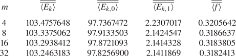
To elucidate the evolution of three-dimensionality in the flow, a case with  $\beta =0.25$ was evolved for
  $Re=400$, well beyond the critical Reynolds number of
  $Re_{cr}=86.85$ predicted in § 5. A plot showing the time evolution of the kinetic energy of each Fourier mode is given in figure 26. The evolution may be divided into three regions. The initial stage (1) represents the short-term dynamics of the flow where a transient rise in the energy of first three Fourier modes can be observed, followed by a linear growth stage (2). The growth rate of the leading Fourier mode here (
 $\mathrm {d} \langle E_{k,1}/2 \rangle / \mathrm {d}t = 0.09080$) matches well with the growth rate predicted from linear stability analysis (
 $\sigma =0.09077$). Stage 3 is where the nonlinear dynamics dominates the flow dynamics. The flow structure in the linear stage (
 $t=215$) demonstrates that a structure consistent with the eigenmodes predicted from the LSA (figure 13a) has emerged from the initial white-noise perturbation. It is also seen that the flow structure holds resemblance to the linear mode even in the weakly nonlinear stage (
 $t=243$) as shown in figure 27.

Figure 26. Evolution of domain integral of kinetic energy ( $\langle E_{k,m} \rangle$) in
  $16$ Fourier modes with time for
  $\beta =0.25$,
  $Re=400$. The dashed bold line represents the energy in the fundamental mode (
 $\langle E_{k,0} \rangle$), energy in the dominant mode (
 $\langle E_{k,1} \rangle$) is given by the solid bold line. The other thin lines represent the energy evolution in the subdominant modes. The transient, linear and nonlinear saturation regions are given by 1, 2 and 3, respectively. A section of region 1 is shown for clarity.

Figure 27. Plots showing the positive (blue) and negative (yellow) streamwise vorticity iso-contours of the flow in the linear and weakly nonlinear stages as it evolves for  $\beta =0.25$,
  $\gamma =2$,
  $\tan (\phi )=0.125$ at
  $Re=400$. The corresponding times are indicated in figure 26; (a)
  $t =215$ (linear stage), (b)
  $t =243$ (weakly nonlinear stage).
To understand the nonlinear departure of the bifurcation from 2-D to 3-D states, the Stuart–Landau equation is used. This model has been widely used to classify weakly nonlinear features of the bifurcation in various flow simulations such as flows past cylindrical (Provansal, Mathis & Boyer Reference Provansal, Mathis and Boyer1987; Dušek, Gal & Frauniè Reference Dušek, Gal and Frauniè1994), spherical (Thompson et al. Reference Thompson, Leweke and Williamson2001), triangular (Ng et al. Reference Ng, Vo and Sheard2018) and toroidal bluff bodies (Sheard, Thompson & Hourigan Reference Sheard, Thompson and Hourigan2004a,Reference Sheard, Thompson and Houriganb), and confined flows such as a 180 degree bend (Sapardi et al. Reference Sapardi, Hussam, Pothérat and Sheard2017). In this model (Landau & Lifshitz Reference Landau and Lifshitz1976), the evolution of the perturbations is modelled as a complex oscillator following:
 \begin{equation} \frac{\mathrm{d} A}{ \mathrm{d}t}=(\sigma+{\rm i}\omega)A - l(1+{\rm i}c)|A|^2A+ \ldots, \end{equation}
where  $A=|A|{\rm e}^{{\rm i}\phi t}$ is the complex amplitude of a signal. The real part of (8.1) thus reduces to (at second order)
 \begin{equation} \frac{\mathrm{d} \log|A|}{ \mathrm{d}t}=\sigma - l |A|^2. \end{equation}
The sign of  $l$ is an indicator of the type of bifurcation of the flow. When
  $l > 0$ (negative slope at
  $|A| \approx 0$), the bifurcation is supercritical, whereas when
  $l<0$, the bifurcation is subcritical.
For the present study, the time history of the leading Fourier mode's energy was used as the signal ( $A$ in (8.1)) and the analysis was carried out for
  $\beta$ in the range
  $0.125-0.5$ at
  $\gamma =2$ and for
  $\beta =0.25$ at an intermediate
  $\gamma =4$. Figure 28 shows plots of
  $\mathrm {d} \log |A|/\mathrm {d}t$ against
  $|A|^2$ for two representative cases. The bifurcation was found to be supercritical for all tested parameter combinations. As the underlying eigenmodes for each of these cases have positive real eigenvalues, the flow undergoes a change to the 3-D state via a supercritical pitchfork bifurcation.

Figure 28. Plots of  $\mathrm {d} \log |A|/\mathrm {d}t$ against
  $|A|^2$ with a negative slope (
 $l>0$) showing a supercritical bifurcation of the 2-D flow to a 3-D state. The growth rate of the corresponding critical eigenmode is represented as a diamond symbol. The cases here have fixed parameters
  $\gamma =2$ and
  $\tan (\phi )=0.125$; (a)
  $\beta =0.25$,
  $Re=400$, (b)
  $\beta =0.5$,
  $Re=100$.
9. Conclusions
This study characterises the flow in a channel with repeated flow-facing wedge-shaped protrusions. Two-dimensional transition in the flow was found to occur through a global complex mode appearing as a wave spanning the streamwise domain length. Increasing blockage ratio, pitch and wedge angle prepones this transition to a lower  $Re$. The onset of three-dimensionality in the 2-D base flow occurs through a stationary mode, well before the onset of the 2-D instability. This holds for the ranges of blockage ratios and pitch values that were considered in this study. Increasing blockage ratio and decreasing pitch both result in a decrease in the critical Reynolds number
  $Re_{cr,{3D}}$. Onset of 3-D effects in the flow is observed mostly near the wedge. The instability is characterised by the formation of a streamwise velocity streak induced by the counter-rotating streamwise vortices near the wedge tip. The lift-up mechanism is found to be responsible for this instability. A PKE budget of the instability modes showed that the production due to horizontal shear in the base flow is responsible for most of the energy gain in all cases. The corresponding locations of maximum shear were in the region ahead and after the wedge tip. The wavemaker region in the flow found though sensitivity analysis is similarly located, further supporting the previous finding from energetics analysis. The significant regions in the flow for placement of an active or passive control mechanism are identified through receptivity and sensitivity analysis. For most of the cases considered, the local pressure gradient component of the endogeneity distribution was found to feature prominently in the total endogeneity field, the sum of which retrieves the growth rate of the global eigenmode, despite its net contribution being intrinsically zero. This emphasises its role in the local endogenous eigendynamics in this system. It is also found that the flow does not aid a significant transient energy growth, unlike similar confined flow set-ups (Blackburn et al. Reference Blackburn, Barkley and Sherwin2008a,Reference Blackburn, Sherwin and Barkleyb; Marquet et al. Reference Marquet, Sipp, Chomaz and Jacquin2008). Three-dimensional flow computations verified the predictions from the LSA, showing that these flows are unstable through a global linear mode. The onset of the 3-D state was also shown to be via a supercritical pitchfork bifurcation for selected parameter combinations.
Supplementary movies
Supplementary movies are available at https://doi.org/10.1017/jfm.2022.200.
Acknowledgements
We are grateful to Professor V. Citro for his helpful communications during our implementation of the BoostConv stabilisation algorithm in our code. S.M. receives an Australian Government RTP and Monash International Tuition Scholarship.
Funding
This research is supported by Australian Research Council Discovery Grant DP180102647 and the high-performance compute facilities of the National Computational Infrastructure (NCI), the Pawsey Supercomputing Centre and the Monash MonARCH machine.
Declaration of interests
The authors report no conflict of interest.
Appendix A. Implementation of constant flow rate
The implementation in the numerical scheme to obtain a constant flow rate is described. Pressure is decomposed into a background pressure gradient part and a streamwise-periodic fluctuating part,  $p=\tilde {p}-F(t)x$; thus the momentum equation (2.2) becomes
 \begin{equation} \frac{\partial \boldsymbol{u}}{\partial t} + (\boldsymbol{u}\boldsymbol{\cdot}\boldsymbol{\nabla})\boldsymbol{u}=F(t)\boldsymbol{e}_x-\boldsymbol{\nabla}\tilde{p}+\frac{1}{Re}{\nabla}^2\boldsymbol{u}, \end{equation}
where  $F(t)$ is a time-varying horizontal forcing function that is dynamically adjusted to obtain a desired flow rate.
Following a similar approach to that described in Karniadakis et al. (Reference Karniadakis, Israeli and Orszag1991), to integrate from time  $n$ to time
  $n+1$, the equations are cast at the future time, the time derivative term is approximated using backwards differencing, and an appropriate-order extrapolation of the nonlinear term to the future time is used. The momentum equation then becomes
 \begin{equation} \frac{\gamma_0 \boldsymbol{u}^{n+1}-\sum_{q=0}^{J_i-1}\alpha_q \boldsymbol{u}^{n-q}}{\Delta t} = \sum_{q=0}^{J_e-1} \beta_q\boldsymbol{N}(\boldsymbol{u}^{n-q}) + F^{n+1}\boldsymbol{e}_x-\boldsymbol{\nabla}\tilde{p}^{n+1}+\frac{1}{Re}\nabla^2\boldsymbol{u}^{n+1}. \end{equation}
Under the third-order scheme, the coefficients are  $\gamma _0=11/6$,
  $\alpha _0=3$,
  $\alpha _1=-3/2$,
  $\alpha _2=1/3$,
  $\beta _0=3$,
  $\beta _1=-3$ and
  $\beta _2=1$.
The solution of the momentum equation is split into four sub-steps, which are identical to the standard scheme, except for the addition of the second sub-step
 \begin{equation} \left. \begin{aligned} \frac{\boldsymbol{u}^*-\sum_{q=0}^{J_i-1}\alpha_q \boldsymbol{u}^{n-q}}{\Delta t} & = \sum_{q=0}^{J_e-1} \beta_q\boldsymbol{N}(\boldsymbol{u}^{n-q}),\\ \frac{\boldsymbol{u}^{**}-\boldsymbol{u}^*}{\Delta t} & = F^{n+1} \boldsymbol{e}_x,\\ \frac{\boldsymbol{u}^{***}-\boldsymbol{u}^{**}}{\Delta t} & ={-}\boldsymbol{\nabla} \tilde{p}^{n+1},\\ \frac{\gamma_0\boldsymbol{u}^{n+1}-\boldsymbol{u}^{***}}{\Delta t} & =\frac{1}{Re} \nabla^2 \boldsymbol{u}^{n+1}. \end{aligned} \right\} \end{equation}
The sequence of calculations is therefore
(i) Extrapolate velocity field to time
 $n+1$ : $\tilde {\boldsymbol {u}}^{n+1}=\sum _{q=0}^{J_e-1} \beta _q(\boldsymbol {u}^{n-q})$.
(ii) Evaluate first intermediate velocity field from
$\boldsymbol {u}^{*}=\sum _{q=0}^{J_i-1}\alpha _q \boldsymbol {u}^{n-q}+\Delta t \boldsymbol {N}(\tilde {\boldsymbol {u}}^{n+1})$.(iii) The forcing is determined by prescribing the target velocity on
$\boldsymbol {u}^{**}$ (note that intermediate velocity fields are upscaled by $\alpha _0$; here, $u_{target}$ is the desired mean horizontal velocity): $F^{n+1}=(\gamma _0 u_{target}-u^* )/\Delta t$.(iv) Form second intermediate velocity field from computed forcing
$\boldsymbol {u}^{**}=\boldsymbol {u}^{*}+\Delta t F^{n+1}$.(v) Obtain pressure from solution of Poisson equation
$\nabla ^2 \tilde {p}^{n+1}=(\boldsymbol {\nabla } \boldsymbol {\cdot } \boldsymbol {u}^{**})/\Delta t$ (this is constructed by taking the divergence of the pressure sub-step, and enforcing the divergence-free constraint on the second intermediate velocity field; pressure boundary conditions are imposed during this calculation).(vi) Evaluate third intermediate velocity field from
$\boldsymbol {u}^{***}=\boldsymbol {u}^{**}-\Delta t \boldsymbol {\nabla } \tilde {p}^{n+1}$.(vii) Obtain the final velocity field from the Helmholtz equations
$\nabla ^2 \boldsymbol {u}^{n+1}-(\gamma _0 Re)/\Delta t \ \boldsymbol {u}^{n+1}=-Re/\Delta t\, \boldsymbol {u}^{**}$ (the velocity boundary conditions are imposed during this calculation).


 Open access