


Background
Over the last 15 years ice-coring in the Northern Hemisphere has shown ice laid down during the last (Wisconsin) ice age has special physical and rheological properties. Koerner (1975) noted that Wisconsin ice from Camp Century and Devon Island has a high dirt, Ca, and Mg content, and consists of fine crystals. Reference PatersonPaterson (1977) reported that bore-hole closure was greatly enhanced for the Wisconsin ice of Devon Island, and Reference HookeHooke (1973) stated that shear tilting of bore holes in the Barnes Ice Cap was a maximum for Wisconsin ice. Also, from two Devon Island Ice Cap cores, Reference Koerner and FisherKoerner and Fisher (1979) showed late Wisconsin ice contained high concentrations of microparticles in anti-phase with the crystal size. In general, it seems that the relationship between very high microparticle concentrations, small ice crystals, and enhanced ice flow is stronger in Arctic ice masses than in the Antarctic where the terrestrial impurity content is of a lower order of magnitude (Reference Cragin, Cragin, Herron, Langway and KloudaCragin and others, 1977; Reference ThompsonThompson, 1977).
Continuous bore-hole closure and δ (18O) profiles through Wisconsin ice of the Agassiz Ice Cap, Ellesmere Island (Reference FisherFisher, 1981), confirmed the earlier spot value from the Devon Island Ice Cap (Reference PatersonPaterson, 1977). More recently, Reference Gundestrup and HansenGundestrup and Hansen (1984), Reference Dahl-JensenDahl-Jensen (1985), and Reference Reeh, Reeh, Johnsen and Dahl-JensenReeh and others (1985) have published analyses of the new Dye 3, Greenland, bore-hole diameter and tilt measurements that confirm enhanced Wisconsin closure and tilt, and further point out that both seem to correlate best with microparticle content. Laboratory tests of Holocene and Wisconsin ice from many drill sites in both hemispheres have assessed the relative importance of flow-enhancement factors related to crystal (c-axis) alignment and impurity content (Reference Shoji and LangwayShoji and Langway, 1984; Reference AzumaAzuma, unpublished).
These laboratory studies confirm the field observations that ice-age ice is rheologically different (weaker) than Holocene ice. However, Reference PatersonPaterson’s (1983) analysis of tilt measurements from the Camp Century, Greenland, and Byrd Station, Antarctica, holes comes to the opposite conclusion; namely, that shear strain-rates for Holocene ice are about three times those of Wisconsin ice. New surveys of these holes, combined with additional surface data, might change his conclusions. Also, extensive studies of a suite of bore holes and cores from Law Dome, Antarctica, show an enhancement maximum above the Wisconsin ice. The enhancement in this case is due to c-axis concentration (Reference Russell-Head and BuddRussell-Head and Budd, 1979) and not impurities.
The present work condenses 7 years of measurements of bore-hole closure and four inclination surveys in a 338 m hole drilled in the Agassiz Ice Cap, Ellesmere Island (Reference Fisher, Fisher, Koerner and PatersonFisher and others, 1983). The resulting strain-rates are compared to other measured quantities δ(18O), dust, crystal size, density, conductivity, Na, Ca, and c-axis orientation.
Reference FisherFisher (1981) and Reference Herron and LangwayHerron and Langway (1982) warned modellers that, because Wisconsin ice is rheologically different from modern ice, their efforts to model ancient ice should not use natural modern flow-law constants.
The Bore Holes and Ice Cap
An ice cap, roughly 16 000 km2 in area, covers the central part of Ellesmere Island between lat. 79° 45’ and 81 °N. Its surface topography is complex and there are nunataks even in the highest parts. The ice cap is drained by glaciers that penetrate the surrounding mountains; the larger ones reach sea-level. The northern part – the Agassiz Ice Cap – is where three cores were recovered in 1977, 1979, and 1984. Hole 77 (338 m deep) is 1 km down-slope from a local ice divide at an elevation of 1700 m. Hole 79 (139 m deep and 27 m higher) is 200 m down the opposite slope of the divide. Hole 84 is within 10 m of the highest point of the local ice dome, as determined by precision levelling, and is about 1.2 km from the 1979 hole and 30 m higher. Down-bore-hole photography and television confirmed that all holes reached the base of the ice. The 12 m and basal temperatures are (–24.2° and –16.7° C), (–22.4° and –19°C), and (–22° and –19.1 °C) for 77, 79, and 84 holes, respectively. Annual precipitation is 0.175 m year-1 ice equivalent. But, about 30% of it (the winter snow) is presently scoured from the 79 and 84 sites (Reference Fisher, Fisher, Koerner and PatersonFisher and others, 1983), and none from the 77 site.
Summer melting, as shown by ice layers in the firn, is slight, on average 3% of the annual precipitation. Only results from the 77 hole are discussed in detail here. A later paper will deal with a comparison of the three holes.
A CRREL thermal drill produced the 77 hole and it was everywhere within 1⁄2° of vertical and, for depths below 200 m, 0.1650 ± 0.0005 m in diameter. Within hours of completion, the hole was partially filled with Arctic diesel oil (density 815 kg⁄m3) to a depth of 60 m below the surface. This oil depth remained constant ±2 m for the 7 years of the study. There is a constant under-pressure (e.g. 0.705 MN⁄m2 at the bottom) closing the hole (MN⁄m2 = 106N⁄m2 = 106 Pa).
The ice-age ice, as defined by very negative δ(18O) values, is confined to a layer between 3.5 m and 8 m above the bed (see Fig. lc). It also has high microparticle concentrations (Fig. lb), small crystal sizes (Fig. 1d), high hole-closure rates (Fig. la), high shear rates (Fig. 1i), and high Ca and Na concentrations (Fig. 1e and f). The (optic) c-axes (Fig. 1j) are highly concentrated already by y = 9 m (y is the distance over the bed) and show little change for older, deeper ice except for one thin section at y = 3 m which consists of very coarse ice.

Fig. 1. a. Diameter of the Agassiz 77 bore hole from bedrock to y = 12 m over bedrock from 1977 (dashed line) every year to 1983. Along the top of this figure are noted the zones referenced in the text and defined in Table I. b. Microparticle concentration,P, of Agassiz 77 core, number (diameter 77 core, number (diameter ≥ 1µm)⁄ml. c. δ(18O), of the bottom 9 m of Agassiz 77 core. d. Crystal size S (mm) of the bottom 8 m of Agassiz 77 core. These were obtained by counting crystal-boundary intersections of a vertical line on a vertical thin section. To obtain “corrected” crystal sizes, one can multiply S by the factor 1.78 (Hilliard, 1970). Note that we use raw crystal sizes throughout this paper. e. Calcium concentration in (ppb) parts (mass) Ca per billion (109) of ice (mass). Measurements were made on a flameless (AA) atomic absorption spectrometer, Perkin-Elmer 603. Sample-preparation procedures followed Reference Cragin, Cragin, Herron, Langway and KloudaCragin and others (1977). f. Sodium concentration in parts per billion (109) by mass for the bottom 9 m of Agassiz 77 core, measured with a Perkin–Elmer 603 AA. g. Conductivity (at 20° C) of liquid samples. Measurements done on a radiometer CDM3. h. Ice density of selected segments of the Agassiz 77 ice core. They were obtained by measuring air-bubble areas of thin sections and assuming that bubble-free ice has a density of 917 kg m-9. Areas were measured on a Metals Research Quantimet image analyser. i. Shear strain-rates over the bottom 12 m of the Agassiz bore hole measured by bore-hole tilt 6 years after drilling. The dotted line is the theoretical shear strain-rate as explained in the text. j. Angular spread (α) of the optic or c-axis over the bottom 9 m of the Agassiz 77 core. This is a measure of half the apex angle of a cone containing 90% of optic axes of ice crystals in a thin section. At 237 m depth this angle is 83°, i.e. completely random c-axis distribution. The average direction of the c-axis over the bottom 9 m is 10° off vertical. This is probably due to bedrock angle which has a value of 17° averaged over several hundred meters up- and down-stream of the Agassiz 77 hole.
Holocene, Wisconsin, and pre-Wisconsin ice are found under nearly identical stress and temperature (–16.9°C) conditions. Thus, one can immediately eliminate these variables as causes of any of the differences in strain-rates.
The close relationship between δ(18O), microparticles, and crystal size (Fig. 1c, b, and d) parallels closely that found in two Devon Island Ice Cap cores (Reference Koerner and FisherKoerner and Fisher, 1979).
Diameters and Closure Rates
Diameters were measured continuously by a Pollak and Skan caliper (Reference Hansen and LandauerHansen and Landauer, 1958) equipped with a pressure-proofed Schaevitz linear-variable differential transformer. The caliper was triggered at the bottom and drawn up by an electro-mechanical winch at 5–10 cm⁄s. Calibration of the caliper was done routinely before and after each run with two known diameters. The diameters for 1977 through 1983 inclusive appear in Figure 1a for the deepest 12 m. This interval has been divided into zones (marked above the top of Figure 1a) by referring to the δ(18O) and micro-particle concentration P (see Table I).
Table I. Zones of the Bottom 12 m of the 1977 Agassiz Hole as Marked on Figure la.

The theory of closure of a cylindrical hole in isotropic ice, as given by Reference NyeNye (1953) and used in Reference PatersonPaterson’s (1977) review paper, is followed here.
The average effective strain-rate έ operating between times t 2 and t 1 changes the bore-hole diameter a(t) and the effective strain-rate is

The effective shear stress τ is
where the net hydrostatic pressure is p and n is the power in the isotropic Glen-body flow law,

Q is the activation energy for ice. For temperatures T ≤ –10°C (44 ≤ Q ≤ 62 – 103 J⁄mol). R is the gas content 8.3143 J deg-1 mol-1. Reference PatersonPaterson (1977) adopted Q =54 kJ⁄mol. Using this Q value and the empirical relationship, he derived between έ and τ (with n = 3) the non-temperature-sensitive constant A o (closure) = 2.662 – 103 (MN⁄m2)-3 s-1. A o depends mainly on impurities, crystal orientation, and size but it also implicitly assumes that the ice is isotropic. Only Glen-body or secondary-type creep is described by Equation (3). To make this explicit, έ2, will be used henceforth for secondary creep-rate.
Diameters were measured every year over the bottom 12 m but sometimes with 2 year intervals for the shallower depths. Here the Agassiz 77 diameters were averaged over 20 cm depth intervals and then further averaged by each zone (Fig, 1a, Table I).
p, and hence τ, is calculated knowing the firn–ice density profile, the oil level, and oil density. These are all well known for Agassiz 77 and for the region of particular interest (0 ≤ y ≤ 12 m) (0.70 ≤ p ≤ 0.71 MN⁄m2). In the same y interval the temperature range is also very narrow (-16.75° ≥ T ≥ -17.0°C).
Highest strain-rates were always in the first year, after which some of the total strain curves (Fig. 2) have cycles of decelerating and accelerating closure strain. Like Reference PatersonPaterson’s (1977) study, we assume that the first year’s strain-rate was mainly transitory or first-order creep denoted έ1. The subsequent decelerations produce strain-rate minima that approach secondary or “Glen-type” creep έ2, and further accelerations produce maximum strain-rates that are assumed to approach tertiary or recrystallization creep, έs (Reference PatersonPaterson, 1977). An example of έ3 creep is the 1981–82 creep for the Wisconsin (WS) ice (Fig. 2).

In practice, the strain-rates, types έ1, έ2, έ3, were assigned using two independent methods:
-
(i) The minimum–maximum method used by Reference PatersonPaterson (1977);
-
(ii) Statistical partition.
(i) Minimum–maximum method to determine creep types
The minimum–maximum method has been described in Reference PatersonPaterson (1977). The only difference from Paterson’s procedure is that, because of the continuity and long duration of this study, multiple minima έ2 and maxima έ3 are available for some of the curves of Figure 2, e.g. for the microparticle-rich Wisconsin ice. For shallower curves (unlettered Holocene curves below H in Figure 2), minima had not been reached by 1983.
The first year’s strain-rates are denoted έ1, the average minimum (or secondary) strain-rates έ2, and average maximum (tertiary) strain-rates έ3. The averages for each zone are plotted for each type of creep versus microparticle concentration P (Fig. 3). The solid lines are least-squares fits to these points. The dashed lines are obtained if the statistical partition method is used to separate strain types.
For all types of creep in the deepest 12 m of the hole, there is a significant tendency for the microparticle-laden, late Wisconsin ice (WS) to deform the fastest and the relatively clean Holocene ice (H) the slowest. The data for B3 and deeper is excluded from Figure 3 because the large number of microparticles P shown in Figure lb for y ‹ 1.5 m are from visible agglomerations, and do not represent the uniform microparticle content in the ice matrix as does P for y › 1.5 m. Similar agglomerations occur in the bottom 0.8 m of the Devon Island Ice Cap cores (Reference Koerner and FisherKoerner and Fisher, 1979).

Fig. 3. Three kinds of closure strain-rates versus microparticle content. The points are for the zones denoted along the top of the figure and defined in Table I. These strain-rate types have been decided on by the minimum-maximum procedure described in the text. a. έ1 is the first-year or transitory strain-rate. b. έ2 is the minimum of Glen-body strain-rate. 3. έ3 is the maximum or tertiary strain-rate. The solid line is a least-squares fit to the points and the dashed line is a least-squares fit through the data when the strain-rate types are decided by the statistical partition method described in the text.
(ii) The statistical partition method for obtaining creep types
The second method partitions all the 20 cm average strain-rates for all the year intervals into a population distribution (Fig. 4). Figure 4 shows three distinct peaks in the έ distribution and the three regions shown can be picked using the minima of the population. These regions are

With these defined as strain-rate categories for έ1, έ2, and έ3, all the strain-rates can be sorted and plotted against the appropriate 20 cm average microparticle concentrations P (Fig. 5a, b, and c). The solid lines on Figure 5 are least-squares fits. These lines appear also in Figure 3 (as the dashed lines).

Fig. 4. The closure strain-rate distribution using alt the strain-rate data 1977-83 averaged on 20 cm depth increments. The three strain-rate types are marked across the top and are defined by the minima in the distribution.
From Figure 3 one can see that the two methods for separating strain-rate types produce very similar regression lines against microparticles for έ1 and έ3 creep. However, the slope of έ2 versus P from the minimum–maximum method is steeper than from the statistical partition method (Fig. 3b). Since the partitition method uses all the έi data and not just the extreme values, one might expect some of the derived έ2 values to include examples of mixed mode creep, i.e. (έ1 + έ2) of (έ2 + έ3).
Reference PatersonPaterson (1977) summarized έ2 closure strain-rate data from Arctic and Antarctic holes by converting the strain-rates to a common temperature of -22°C using an activation energy of Q = 54 kJ⁄mol. In order to compare directly with his work (Reference PatersonPaterson, 1977, fig. 5), we used the same Q value here.

Fig. 5. Three types of closure strain-rate as found using the statistical partition procedure. The points are the 20 cm averages of strain-rate plotted against microparticle concentration P. The open circles are for ice containing visible agglomerations of dirt. These open-circle points are not used in forming the least-squares lines that appear. a. Transitory-type strain-rate έ1 b. Glen-type strain-rate έ2 c. Tertiary-type strain-rate έ3.
Paterson’s log (έ2) versus log (τ) plot for all previous bore-hole closure measurements has a regression line (at T = -22 °C) that gives
with έ2 in s-1 and τ in MN⁄m2. This line is reproduced in Figure 6 along with the Agassiz 77 hole έ2 data (0 < y < 12 m) shifted to –22°C for each zone. The Holocene points (H) fit the Paterson line but the older parts of the hole close significantly faster with the dirtiest part of late Wisconsin (WS) having closure strain-rates nearly three times the Holocene values, H.
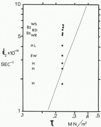
Fig. 6. Logarithmic plot of minimum or Glen-type έ2 closure strain-rates for the zones in the bottom 13 m of the Agassiz 77 hole versus effective stress τ. The zones are as in Table I and Figure 1a. The measured strain-rates have been shifted to -22° C to be directly comparable with Reference PatersonPaterson’s (1977. fig. 5) empirical line for έ2 versus τ from non-ice-age zones of other bore holes.
Ice in the 0 < y < 12 m range has a highly concentrated c-axis alignment about 10° off vertical. The c-axis concentration α as expressed in Figure lj is half the apex angle of the cone that contains 90% of the measured optic axes. The definition of α is the same as used by Reference Herron, Herron, Langway and BruggerHerron and others (1985). This concentration favours shear deformation and tends to hinder bore-hole closure (Reference Thwaites, Thwaites, Wilson and McCrayThwaites and others, 1984). There is little variation in the c-axis alignment in the bottom 12 m (Fig. lj) and the enhanced closure for ice with a high microparticle content is not evidently reflected in variations in c-axis. This was also the case for the Devon Island Ice Cap cores. Of course, the value of A 0 in Equation (3) can be increased by increasing the c-axis alignment and this has been called c-axis enhancement (Reference Shoji and LangwayShoji and Langway, 1984).
The A 0 enhancement in the microparticle-rich pre-Holocene ice which is not due to variations in c-axis fabric we call rheological enhancement. Reference Shoji and LangwayShoji and Langway (1984), from laboratory testing of natural ice, have separated c-axis enhancement (fabric factor) from rheological enhancement (remnant or impurity factor). Their impurity factors for Wisconsin ice are in the range from 3 to 6. Also, Reference Reeh, Reeh, Johnsen and Dahl-JensenReeh and others (1985) and Reference Dahl-JensenDahl-Jensen (1985) have reported rheological enhancement in the 3-4 range from the Dye 3, Greenland, bore hole.
Bore-hole closure strains are “unnatural” in that the bore hole was suddenly and arbitrarily put there. The closure is consequently not along favourably aligned planes. Also, the effective stresses in closure situations tend to be considerably larger than those usually encountered in the slow undisturbed creep of ice. In addition, since the total strains and even crystallographic alignment and creep type are functions of radial distance from the centre of the hole and time since drilling, the actual meaning of the measured strain-rate at the hole’s wall is not clear. Nevertheless, since the enhancements we obtained from closure are relative and from a narrow depth range, we feel they are real.
Bore-Hole Tilt
If a site is over four times the ice thickness (Reference PatersonPaterson, 1981) from the divide, then one can approximate ice deformation by a simple shear model (Reference NyeNye, 1952). If the x coordinate is measured in the direction of flow, the shear stress at depth Z is
and this shear stress is related to the shear strain-rate by
with αs the surface slope (assumed small), ρ the density of ice, and g the acceleration due to gravity. We take n = 3. A = A 0exp(–Q⁄RT) as in Equation (3) where A 0 (tilt), the temperature-independent factor, is 4.2919 – 105 (MN⁄m2)-3s-1 or (1.35 – 10-5 Pa-3 a-1). This value for A 0 is derived from the recommended cold-ice activation energy Q = 60 kj⁄mol and Paterson’s recommended value for A for polycrystalline ice at T = -10°C (i.e. A = 5.2 – 10-7 (MN⁄m2)-3s-1 (Reference PatersonPaterson, 1981). The simple shear model, Equations (4) and (5), works at sites like Dye 3, Greenland, which is about ten times the ice thickness from the divide, but it should not be used for a site like the Agassiz 77 bore hole which is only four thicknesses from the divide. Under such circumstances, the longitudinal strain-rate έ xx must be included and deformation can be estimated by (Reference NyeNye, 1959) the equations
with the effective strain-rate έ here given by
In practice, έ xx is estimated and Equations (6) and (7) are solved for έ xz at a given ice depth Z (and temperature) by iteration on έ, e.g. Reference PatersonPaterson, 1983.
The tilting rate ![]() of an initially vertical bore hole is equal to twice the shear strain-rate έ
xz
and is approximated by (Reference PatersonPaterson, 1983)
of an initially vertical bore hole is equal to twice the shear strain-rate έ
xz
and is approximated by (Reference PatersonPaterson, 1983)

where u is the x component of velocity. Equations (4) through (7) assume that the ice is isotropic.
Tilting rates and subsequent shear strain-rates can be measured by logging the inclination of bore holes. When the inclinations are small,

where ![]() is the initial inclination (in radians) and
is the initial inclination (in radians) and ![]() after time Δt.
after time Δt.
Four angular inclination surveys of the Agassiz 77 hole have been made. Immediately after drilling in 1977 and again in 1979, the hole was logged under contract with Eastman Oil Well Survey Co. Limited and Sperry–Sun of Canada Limited, respectively. The long 4 m tool apparently only penetrated to 328 m in 1977 and to 322 m in 1979, although the hole is 338 m deep, and there was no geometric reason for failure to reach the bed. The 1977 survey showed that the hole was initially everywhere within ½° of vertical.
In 1982 and 1983, we conducted our own inclination surveys using a Pajari inclinometer (Pajari Instruments Ltd of Canada) mounted on a 1 m long tool. The two earlier surveys used battery-powered gyros to give angular inclinations to 1’ and azimuth to 1°. The Pajari instrument is a self-locking pendulum and magnetic compass device that gives azimuths and inclinations to 1°. The limiting factors in all these surveys tended to be the spring-centering accuracy and depth measurement. So, while the Pajari surveys only gave angles to 1°, we feel these inclination results are the more reliable because:
-
i. The inclinations were done 6 years after drilling and were as large as 6°.
-
ii. The azimuths of the surface velocity derived from the Pajari surveys agreed with the 1979 survey.
-
iii. While the Pajari tool was only 1 m long (giving the required resolution), many runs each year were done to ensure repeatability at each depth. Runs were also done with a 2 m tool. No repeat runs were made in the 1977 or 1979 surveys of the 77 hole.
-
iv. The Pajari surveys unequivocally reached bedrock as the bottom had previously been marked on the inclinometer cable using a very narrow weight which allowed the observer to feel the weight change on the cable when bedrock was reached. All depth/inclinometer measurements were then made with reference to the bed and not the surface. Contrasting with this method, the 1977 and 1979 contract surveys measured depth from the surface using cable-length friction counters attached to an oily cable; slippage almost certainly occurred. The contract surveys therefore reached bedrock but gave incorrect depths. The alternative explanation that both 1977 and 1979 survey tools jammed in the hole before reaching bedrock is unlikely. There is no reason for jamming in 1977 as the hole had just been drilled, was within ½° of vertical (drill-mounted Pajari measurements during drilling attested to this), and was everywhere 16.5 cm in diameter. The only location for jamming to have occurred during the 1979 survey was at the Wisconsin/Holocene transition where hole curvature reached maximum values. However, this transition is 8 m above the bed and not the 16 m reported.
The shear strain-rates derived from the contract surveys agree well with the Pajari results except in the depth range 280–310 m, where the contract strain-rates are three times larger. If, as we believe, the commercial depth measurements were in error, and both the 1977 and 1979 surveys actually reached bedrock, then the different shear strain-rate sets are everywhere in reasonable agreement. For all these reasons, we adjusted the contract survey depths assuming that they actually reach bedrock. The Pajari results are used from Z = 312 to 338 m and the contract results from 0 to 310 m. Figure 7 summarizes all the shear or tilt strain-rate measurements and Figure li details the bottom 12 m.

Fig. 7. Tilt or two times the shear strain-rate of the Agassiz 77 bore hole verus real depth; crosses are values from a “professional” survey made in 1978; open circles are from the Pajari survey of 1982; and the line is from the Pajari survey of 1983.
Estimates of theoretical tilt strain-rates έxz were made using Equations (6) and (7) and the following approximation to the longitudinal strain-rate.

where x is distance down the flow line and Z is ice-equivalent depth. This two-line approximation for έxx is based on
-
(i) A measured surface value
 A depth-averaged value
where ū is the ice-depth averaged velocity (0.38 m a-1), u
s the surface velocity (0.45 m a-1), H the thickness in ice equivalent (321 m), and ∂Zs/∂x the surface slope (0.021 rad).
A depth-averaged value
where ū is the ice-depth averaged velocity (0.38 m a-1), u
s the surface velocity (0.45 m a-1), H the thickness in ice equivalent (321 m), and ∂Zs/∂x the surface slope (0.021 rad). -
(ii) An estimate of έxx near the bed, at Zice = 313 m.
where (∂u/∂Z)b = -8.73 – 10-3a-1 comes from the inclination measurements and the bottom slope averaged over 900 m of flow line is (∂Z/∂x)b= 0.31 rad.
 where ū is the ice-depth averaged velocity (0.38 m a-1), u
s the surface velocity (0.45 m a-1), H the thickness in ice equivalent (321 m), and ∂Zs/∂x the surface slope (0.021 rad).
where ū is the ice-depth averaged velocity (0.38 m a-1), u
s the surface velocity (0.45 m a-1), H the thickness in ice equivalent (321 m), and ∂Zs/∂x the surface slope (0.021 rad).
With these theoretical estimates of έxz, the ratios (έxz measured/έxz theory) are calculated and taken to be (A0 measured/A0 theory), a measure of the shear-enhancement factors (SEF).
Well above the Wisconsin ice at Zice = 280, we calculate SEF = 1.0. Figure 8b gives SEF over the bottom 12 m. The Holocene ice has an SEF near 1 and the largest SEF of 3 occurs in the late Wisconsin ice. The Holocene SEFs of 1 seem to indicate little influence of c-axis concentration which shows a gradual strengthening of fabric with increasing depth in the Holocene ice.

Fig. 8. Enhancement factors (measured creep/theoretical or expected creep) for (a) closure strain-rates, i.e. closure-enhancement factor or CEF; (b) shear or tilt strain-rates, i.e. shear-enhancement factor SEF.
Comparison of Tilt- and Closure-Derived Enhancement Factors with other Variables
Enhancement factors for secondary type strain-rates έ2 derived from the bore-hole closure measurements are found for each zone of Figure la. The “normal” or theoretical έ2 values come from Patersons’s empirical line reproduced in Figure 6. The resulting closure-enhancement factors, CEFs, over the bottom 12 m of the Agassiz 77 hole are shown in Figure 8a along with the tilt-derived shear strain-rate enhancement factors, SEFs in Figure 8b. The two curves of Figure 8 are remarkably similar, with two broad enhanced-flow maxima at 0-2 m over the bed (zones B3, B5, and deeper) and between 4.5 and 8.0 m over the bed (zones WR, WS, and RD, i.e. late Wisconsin ice). The WS or late Wisconsin ice has the largest SEF and CEF. Comparison of the flow-enhancement factor plots of Figure 8 with other measurements allows elimination of some possible causal variables.
c-Axis Alignment
For the Holocene ice just above the Wisconsin in (12 > y > 8 m), SEF = 1.5 with α = 35° and for shallower Holocene ice (e.g. y ~ 44 m), SEF = 1.0 and α = 85°. Evidently, the SEF changes are not strongly dependent on α. This conclusion seems to substantiate that of Dahl-Jensen (1985) from Dye 3 data, and Reference Russell-Head and BuddRussell-Head and Budd (1979) from the Law Dome study. Furthermore, the variations in SEF between 0 and 8 m over the bed can have little to do with c-axis alignment. Crystal c-axis measurements of seven thin sections show that the c-axis fabric is very strong and quite stable for the interval 0-10 m over the bed (Fig. lj). There are four narrow bands of very large crystals 4 mm or larger 2 < y < 3.5 m over the bed. Three of the bands are less than 10 cm thick but contain crystals up to 7 mm. Two sections that include some of these very narrow bands have c-axis concentrations typical of the rest of the bottom 12 m. The fourth band is about 30 cm thick and the thin section from it had a 90% c-axis containment cone with a half-angle of 73 °! However, because of their size, there were too few crystals in this band to allow much significance to be placed on this α value.
If the late Wisconsin (WS) SEF maximum was due mainly to c-axis concentration, then the closure rates should have a minimum there because shear tilting and closure cannot utilize the same easy glide planes (Reference Thwaites, Thwaites, Wilson and McCrayThwaites and others, 1984). In fact, the opposite is true (Fig. 8).
Similarly, in the Devon Island Ice Cap and Dye 3 cores, there is little change in the c-axis fabric from early Holocene to late Wisconsin ice but there is a large enhancement-factor change (Reference PatersonPaterson, 1977; Reference Dahl-JensenDahl-Jensen, 1985; Reference Herron, Herron, Langway and BruggerHerron and others, 1985).
δ(18O)
Large enhancements are not only associated with very negative (ice-age) δ(18O) values (Fig. lc). The bottom 2 m of ice has large SEFs and CEFs but relatively positive (interglacial) δ(18O) values.
Density
Reference HookeHooke (1973) noted that enhanced tilting in the Wisconsin ice of the Barnes Ice Cap occurs in ice that is very bubbly and consequently has low density (870 kg m-3). Reference BoutronBudd (1969) has suggested such low-density ice is weaker. This explanation cannot be used for the Agassiz Ice Cap data, because the densities for one of enhancement maxima (the late Wisconsin zone WS) is only marginally lower (900 kg/m3) than the surrounding ice (910kg/m3). The density for the other enhancement maximum (bottom 2 m of ice) is completely typical (see Fig. lh).
Impurity Content
The measured impurities include Na, Ca, P (insoluble microparticles < 1 μm in diameter), and σ (liquid conductivity) (Fig. If, e, b, and g), respectively. The conductivity measures the total soluble impurity: salts + acids (Reference HammerHammer, 1977).
Because calcium is clearly a significant constituent of the microparticles, we can simply refer to the micro-particles (Reference Cragin, Cragin, Herron, Langway and KloudaCragin and others, 1977; Reference BoutronBoutron, 1979). By comparing the enhancement factors of Figure 8 with the impurity content, one sees that the enhancement does not follow either the total soluble-ion concentration or the Na, whereas it does correlate well with the microparticles. Thus, of the variables measured, we are left with microparticles as being most closely connected statistically to enhancement factors. Reference Gundestrup and HansenGundestrup and Hansen (1984) found a similar correlation between tilt and microparticles in the Dye 3, Greenland, bore hole (see Fig. 10)

Fig. 10. a. Measured and theoretical lilt or shear strain-rates for the Dye 3 bore hole, south Greenland. b. Shear-strain enhancement, SEF, factor for Dye 3. c. Microparticle or dust concentration in Dye 3. d. Crystal size in Dye 3 core.
The high microparticle mass contains a large calcium contribution (Fig. lc). This is also true for the Dye 3 core and has been used by Hammer and others (1985) to explain the alkaline nature of these parts of the core from Dye 3. The (ECM) solid conductivity is very low for this ice (Hammer and others, 1985) and Hammer (persona! communication) believes that this is a key element in explaining the enhancement-factor profiles.
Crystal Size
The Agassiz 77 crystal size (Fig. 1d) has a marked relationship to microparticle content (Fig. lb), with high microparticle concentrations in ice with small equant crystals. The same relationship exists for the Devon Island Ice Cap cores (Reference Koerner and FisherKoerner and Fisher, 1979). Figure 9 shows In(S/S٭) plotted against In(P/P٭) where S is the uncorrected crystal diameter (mm) and P is the microparticle concentration (number >1 μm/ml). S٭ is the minimum S (1 mm) and P٭ is the minimum P (8000/ml). The points use 20 cm averages of S and P for the bottom 8 m of ice. Crosses show Agassiz 77 and solid circles the Devon Island Ice Cap cores. The open circles and circled dots are points for the bottom 2 m and 1 m of the Agassiz Ice Cap and Devon Island Ice Cap, respectively. This ice contained the agglomerations of visible particles that give rise to the very high P peaks that make the 20 cm averages unusable. We feel it is the microparticles uniformly distributed in the ice that are important here.

Fig. 9. Natural logarithmic plot of crystal size (uncorrected) S versus microparticle concentration P for the bottom 8 m of the Agassiz 77 core (crosses) and Devon Island Ice Cap cores (solid circles). The open circles are in the bottom 1.5 and 0.8 m, respectively, of Agassiz 77 and Devon Island ice that contained visible dirt agglomerations. These points were not used to calculate the two least-squares lines shown. S٭ is the smallest crystal found. S٭ =1 mm and P٭ is the minimum dirt concentration. P٭ = 8000 (number with diameter ≥ 1μm/ml). It would seem that below a certain threshold of about P = 15 000 there is no relationship between P and S.
The two lines in Figure 9 are least-squares lines that excluded the circle points. The low-dirt region line is (figure 9)

FOR 15 000 < P < 36 000 (>1 μm/ml) and for "dirty" ice

for 36 000 ≤ P (>1 μm/ml).
The cersion of Equation (10) and (11) in Reference Koerner and FisherKoerner and Fisher (1979) is incorrect due to a printing error.
The Devon Island late Wisconsin ice also has a large (›3) closure enhancement (Reference PatersonPaterson, 1977), where there is high microparticle concentration and small crystals but no change in c-axis alignment (Reference Koerner and FisherKoerner and Fisher, 1979) For P ≤ 15 000, there appears to be no relationship at all between crystal size and microparticle concentration. This might explain why the cleaner Antarctic ice (Reference ThompsonThompson, 1977) shows little or no correlation between crystal size and microparticles.
Dye 3: Tilt Enhancement, Microparticles, and Ice Crystals
The Dye 3 bore-hole measurements (Reference Gundestrup and HansenGundestrup and Hansen, 1984) were used to calculate shear strain-rates έxz using Equation (9), The expected or theoretical éxz values were calculated using Equations (4) and (5) with αs = 0.00480 rad (Reference Gundestrup and HansenGundestrup and Hansen, 1984) and with A0 and Q equal to the Agassiz Ice Cap shear values. The enhancement ratio, as before, is (measured/theoretical) and is denoted Am/A0, Am being the “measured” value of the A0 constant.
The measured shear strain-rates (Reference Gundestrup and HansenGundestrup and Hansen, 1984), enhancement factor, microparticle mass (Hammer and others, 1985), and crystal size (Herrón and others, 1985) appear in Figure 10. Virtually the same enhancement-factor profile was obtained independently by Dahl-Jensen (1985). The Dye 3 enhancement, microparticle concentration, and crystal size (Fig. 10) bear the same relationship to each other as they do in the Agassiz 77 and Devon Island cores. The Dye 3 late Wisconsin SEF maximum of 3.5 is somewhat larger than the Agassiz SEF of 2.9 and CEF of 2.7. The Dye 3 e-axis concentration profile (Herrón and others, 1985) is similar to that of the Agassiz 77 core with Wisconsin half-cone angles of about 25° and early Holocene of about 35°.
The Dye 3 bore hole was filled with a denser liquid than Agassiz 77 (Reference Gundestrup and HansenGundestrup and Hansen, 1984), resulting in a net over-pressure and hole-widening with time. Qualitatively, one can see that the Dye 3 bore hole opened more rapidly for the Wisconsin and/or “dirty” ice (Reference Gundestrup and HansenGundestnip and Hansen, 1984). But, because of a complicated liquid-density profile, long drilling time, and missed field seasons in the diameter logging, no quantitative measure of “closure” enhancement can be made.
The Anisotropy Problem
Like Dahl-Jensen (1985) and Reference Russell-Head and BuddRussell-Head and Budd (1979), we found that despite the increase in vertical c-axis concentration with depth, a single set of constants A0 and Q (see Equations (5) and (6)) in a non-linear (n=3)° flow law provided an adequate description of bore-hole tilt for post-Wisconsin ice. This would seem to contradict Reference LileLile’s (1978) laboratory strain tests on 200 m deep samples from Law Dome core SGF. This ice has small α values and near-vertical c-axes. For simple shear stress <0.04 MN m-2 (octahedral) and high temperatures (-6° C), the c-axis enhancement is 2.8 (Lile’s sample 200 Fl). Lile’s c-axis enhancement ratio is with respect to an equivalent piece of laboratory-produced isotropic ice. From laboratory tests on SGF cores, Russell-Head and Budd calculated c-axis enhancement factors of up to four in post-Wisconsin Law Dome ice.
For ice caps, the flow-law constants Q and A0 are usually chosen to produce a best fit to measured bore-hole tilt or tunnel-closure data. Since both temperature and c-axis concentration tend to increase together with depth, possibly both the c-axis and temperature enhancement are lumped together in the choice of the constants. This would explain why there seems to be no c-axis enhancement when one calculates the expected strain-rates using the best-fit A0 and Q constants.
Possibly, a clear example of c-axis enhancement can be seen in the deep ice of the Agassiz 77 core where there is a high near-vertical c-axis concentration. This ice (early Holocene and older) is well oriented for the shear responsible for bore-hole tilting and badly oriented for bore-hole closure. The A0 constants for tilt and closure of this deep ice have a ratio of 10, i.e. A0(tilt)/A0(closure), in agreement with Reference PatersonPaterson (1981) and Reference LileLile (1978). The laboratory tests of Reference LileLile (1978) on SFG Law Dome samples 200F1 and 200F3, which were shear tests in the most favoured plane and 45° to it, gave a ratio of A0(200F1)/A0(200F3)=12.
The A0(tilt)/A0(closure)= 10 ratio is constant for early Holocene ice and deeper (right through the Wisconsin and basal ice) in spite of the fact that the non-c-axis enhancements SEF and CEF vary between 1 and 3 (see Fig. 10).
Conclusion
Closure and shear enhancement for microparticle-laden and/or ice-age ice from Agassiz 77, Devon Island, and Dye 3 does exist and, where known, is about three. From the Agassiz 77 closure data, it appears that transient έ1 and tertiary έs creep-rates are also enhanced by the presence of high particle concentrations. Of the quantities measured on the Agassiz 77 cores, microparticle concentration (or Ca) correlated best with enhancement factors. Also, for the microparticle concentrations greater than 15 000 (>lμm/ml), there is a clear inverse relationship with crystal size for Agassiz and Devon Island. In addition, there is a visible inverse relationship for the Dye 3 cores between crystal size and microparticle mass. The lack of a clear relationship between microparticles, crystal size, and flow enhancement in Antarctic ice is probably because this ice is an order of magnitude “cleaner” in microparticles and rarely gets above the threshold value.
There can be little doubt that there is a rheological enhancement factor of up to three that is related to impurities in natural ice, particularly in Northern Hemisphere late Wisconsin ice. In future, modellers should keep this in mind when reconstructing ancient ice sheets, that would consist largely of microparticle- (calcium-rich) laden ice.
Acknowledgements
W.S.B. Paterson’s critical review of this paper and his earlier work on this topic have been invaluable, Discussions and data exchange with N. Reeh, D. Dahl-Jensen, and N Gundestrup have been very helpful to us.


