


Physical Parameter Values and Notation

1. Introduction
The down-slope sliding of large ice sheets is an intrinsically thermo-mechanical problem, since the shear deformation of ice is strongly controlled by its temperaturedependent rheology. Accordingly, viscous dissipation can play an important role in modifying the movement of ice sheets. Reference Clarke, Clarke, Nitsan and PatersonClarke and others (1977) and Reference Yuen and SchubertYuen and Schubert (1979) drew attention to the fact that shear heating could cause instability in ice flows; Reference Schubert and YuenSchubert and Yuen (1982) suggested that the East Antarctic ice sheet could be vulnerable to this type of creep instability. All of these previous efforts have been based upon arguments drawn from linear stability analyses.
The time-scale for the growth of shear-heating instability in creeping ice sheets is of particular significance in determining the potential physical relevance of the instability. In order for shear-heating instability to exert an influence on the climate system, the instability should grow and significantly affect the dynamics of the ice sheet in a time comparable to or less than the time-scale of the basic glacial cycle 0(105 year). Shear-heating instability in ice is a type of explosive instability that also occurs in combustion phenomena. The instability occurs suddenly or explosively after a prolonged period of simmering or slow monotonic growth. Thus the time-scale associated with the non-linear evolution of an explosive-type instability generally exceeds the growth time predicted by linear theory (Reference Buckmaster and LudfordBuckmaster and Ludford, 1983, chapter 3). A non-linear calculation is therefore required to determine quantitatively the simmering time before the onset of explosive instability in creeping ice sheets. The determination of these times is the primary purpose and contribution of this paper.
We begin in section 2 with a description of the one-dimensional model (Reference Schubert and YuenSchubert and Yuen, 1982) of an ice sheet creeping down-slope and give the equations governing the evolution of shear-heating instability. The manner in which the instability is triggered is discussed next and we conclude the section by describing the numerical methods used to monitor the non-linear growth of an instability. Section 3 presents the numerical results and discusses how the onset time for explosive instability depends on the environmental and rheological parameters of the model. It turns out that the time to get explosive instability depends very sensitively on the rheological parameters of ice. Instability time-scales can differ by orders of magnitude for variations in the rheological parameters encompassed by uncertainties in our knowledge of the creep properties of polycrystalline ice. We close in section 4 with a summary and a discussion of the implications of our results for the occurrence of shear-heating instability in real ice sheets
2. Governing Equations and Numerical Methods
We will employ a simple one-dimensional model (Reference Clarke, Clarke, Nitsan and PatersonClarke and others, 1977; Reference Schubert and YuenSchubert and Yuen, 1982) to investigate finite-amplitude shear-heating instabilities. Admittedly, these models do not include factors such as the horizontal advection of cold ice and the reduction of the shear stress upon a local increase in temperature. Both of these are stabilizing influences. Nonetheless, our studies should yield valuable insight into the physical mechanisms at work, since the set of two-dimensional, thermo-mechanical boundary-layer equations may contain some serious numerical difficulties (Reference MorlandMorland, 1984). In the future it should be feasible with supercomputers, like the CRAY-2, to solve with fine meshes the complete two-dimensional set of thermo-mechanical equations. This would obviate the need for approximating solving the boundary-layer equations with their attendant problems of specifying the correct up-stream conditions.
We will consider the motion of a horizontally infinite ice sheet with thickness h inclined at an angle α with respect to the horizontal. The coordinate system is oriented with the y-axis perpendicular to the slope. The ice surface is at y = h and the base is located at y = 0. The distribution of shear stress τ in this model is
where ρ is the density of ice and g is the gravitational acceleration. The approximate one-dimensional equation governing the temporal evolution of the temperature T is

where t is the time, k is the thermal conductivity, k is the thermal diffusivity, E * is the activation energy for the creep of ice, A is the pre-exponential constant in the ice rheological law, R is the universal gas constant, and v is the ice velocity in the direction perpendicular to the slope. We take v(y) to be a linear function of y, v(y) = v 0 y/h; positive v 0 signifies accumulation. We will consider only accumulation since this condition stabilizes the ice sheet (Reference Clarke, Clarke, Nitsan and PatersonClarke and others, 1977). Equation (2) gives the change of temperature with time as the net result of conduction, advection, and viscous dissipation. It is solved subject to the boundary conditions

where q b is the geothermal heat flux entering the bottom of the ice sheet.
The down-slope flow velocity is determined from the creep law of ice, where we have taken the Glen’s power law with the power-law index n = 3 and the Arrhenius rate factor (Reference PatersonPaterson, 1981, chapter 3).

This equation is integrated subject to the condition
The third-order system in Equations (2)–(6) represents a standard two-point boundary-value problem that can be solved by straightforward numerical techniques (Reference Yuen and SchubertYuen and Schubert, 1979). Solutions to the steady-state version of Equations (2)–(6) have been obtained by Reference Yuen and SchubertYuen and Schubert (1979) and Reference Schubert and YuenSchubert and Yuen (1982).
The physical constants used in most of the calculations are listed at the beginning of this paper. The rheological parameters E * and A are taken from Reference Clarke, Clarke, Nitsan and PatersonClarke and others (1977) and Reference PatersonPaterson (1981, chapter 3). We have also varied A and E * in our calculations, as the pre-exponential parameter may be uncertain by creep data at ice shelves. We have varied these parameters in order to understand the physical effects from uncertainties in these parameters. For example, below -10°C, E * could vary between 42 and 84 kJ mol-1 (Reference PatersonPaterson, 1981, chapter 3).
Due to the exponential dependence of the viscosity upon the temperature, the non-linear system in Equations (2)–(6) yields multiple steady-state solutions (Reference Clarke, Clarke, Nitsan and PatersonClarke and others, 1977; Reference Yuen and SchubertYuen and Schubert, 1979). Figure 1 shows an example of the multiple steady states. For a given equilibrium ice thickness there exist two states with different basal temperatures and down-slope surface velocities. The solid parts of the curves delineate the sub-critical solutions while the dashed parts of the curves (drawn schematically) indicate the super-critical solutions. The super-critical branch cannot be reached by a forward integration of the complete time-dependent Equations (2)–(6). It can only be obtained by treating the steady equations as a non-linear two-point boundary-value problem. On the other hand, the sub-critical branch can be arrived at by treating the equations either as a parabolic system with the time dependence present in Equation (2) or as an elliptic system with the time-derivative in Equation (2) omitted. We have found that the nature of the multiple steady-state solutions does not come from the power-law dependence of the rheology. Rather, it is the temperature-dependent rheology by itself which is responsible for these shear-heating instabilities.

Fig. 1. Multiple steady stales in the down-slope creep of a constant-thickness ice sheet. Basal temperature and surface velocity are plotted as functions of ice thickness. The critical height is denoted by hc; for h > hc there are no steady-state solutions. Rheological and physical parameters are taken from the text.
We observe in Figure 1 that there is a maximum height h c above which no steady-state solutions can exist. Super-critical solutions (dashed curves) have bottom temperatures greater than the melting temperature of ice. At this stage, the model is no longer valid. Hence, it is only the sub-critical branch which is of interest here. Reference Schubert and YuenSchubert and Yuen (1982) have called attention to the closeness of these critical heights to the present-day ice thickness in East Antarctica. They argued that a finite-amplitude creep instability might be possible through a sudden increase of the ice thickness above h c. However, the growth times of these instabilities were not evaluated. Our task in this paper is to conduct a thorough numerical investigation of the growth times of these instabilities. They will be seen to have explosive character similar to instabilities encountered in combustion (e.g. Reference Kassoy and PolandKassoy and Poland, 1980). However, the explosion can be preceded by a long period of simmering or slow monotonic growth.
We consider a basic steady sub-critical state with thickness h 0 and at t = 0 suddenly change the ice-sheet thickness by Δh. The total ice thickness h in Equation (2) is then h 0 + Δh. Other ice-thickening histories can be investigated but the sudden increase represents a limiting case that is expected to yield the most sensitive ice-sheet response. Our model does not allow the ice sheet to thin in response to the imposed abrupt increase in thickness. Because thinning would tend to quench the shear-heating instability (Reference Fowler and LarsonFowler and Larson, 1980), our results provide only a lower bound on the time to explosive instability. Nevertheless, our calculations are important because they delineate the conditions under which explosive instability could conceivably occur on a fast enough time-scale to be a potentially significant climatic factor. Incorporation of the ice-thinning effect is necessary, however, for a complete and final assessment of the potential physical importance of shear-heating instability. For marching the temperature equation in time, an initial temperature profile must be supplied. The initial thermal profile is divided into two parts. The temperature of the newly added ice of thickness Δh is taken to be isothermal at the surface temperature T 0. Below this layer the initial temperature follows the thermal distribution given by the steady-state solution with an equilibrium height of h 0. The accumulation rate is held constant except for the sudden thickening that occurs at t = 0. Thus, v = v 0 y/h for the initial state computation of T with h = h 0 and v is given by -v 0 y/(h 0+Δh) in the computation of T for t > 0.
We have employed a partial differential equation solver developed by Reference SewellSewell (1982). The program approximates spatial derivative operators using Hermite cubic splines and marches in time using the method of lines. The coefficients of the basis functions are integrated as an initial value system using a stiff differential equation integrator. The accuracy of the program has been tested by calculating the linear growth rates of the thermal disturbances and comparing them with the results of Reference Clarke, Clarke, Nitsan and PatersonClarke and others (1977). Typically, 30 to 40 unevenly distributed nodal points are adequate for accurate solutions. Nodal points must be concentrated in the basal shear layer to resolve the large spatial gradients therein. At least ten points have been placed in the shear layers of the cases reported here. The time-discretization error is maintained below 10-3 based on a relative-error criterion.
3. Numerical Results
3.1. Time for the onset of explosive instability
Figure 2 shows typical time histories of the basal temperature T b for three activation energies (50, 60, and 70 kJ mol-1) and three values of Δh (1, 3, and 8 km), Other parameter values are given at the beginning of this paper and in all cases h 0 = 2 km. For shear-heating instability to occur, h 0 + Δh must exceed h c. Because h c increases with E * for the cases considered in Figure 2, Δh must be increased with E * to trigger instability. With h 0 = 2 km and Δh = 1 km, instability would not occur for E * = 60 and 70 kJ mol-1. Similarly, with h 0 = 2 km and Δh = 3 km, instability would not occur for E * =70 kJ mol-1. Though this is the main rationale for choosing different values of Δh in Figure 2, the calculations nevertheless present us with the opportunity of studying how the growth of the instability depends on Δh. It should be noted here that these values for Δh are used here for the purpose of illustrating the amount required for obtaining an instability. One should, in no way, consider that large values of Δh, say 3 km, are at all possible. These values of Δh are meaningful when viewed in the light of finite-amplitude perturbation analysis.

Fig. 2. Temporal evolution of the basal temperature Tb following a sudden increase in ice thickness, (a) E* = 50 kJ mol-1, initial height h0 = 2 km. critical height hc = 2.15 km, Δh= 1 km; (b) E* = 50 and 60 kJ mol-1, hc for 60 kJ mol-1 = 4.6 km, h0 = 2 km, Δh = 3 km; (c) E* = 50, 60, and 70 kJ mol-1, hc for 70 kJ mol-1 = 9.1km. h0 = 2 km, Δh = 8 km. Other parameters are from the text
Initial basal temperature depends on E * and it can be seen particularly clearly in Figure 2c that T b initial is higher the lower the activation energy. Figure 2 also shows that for a given Δh the time for the onset of explosive instability is shorter for smaller E *. A difference in E * of just 10 kJ mol-1 can mean a change of two orders of magnitude in the explosion-triggering time (Fig. 2b and c). For Δ = 1 km, only the state with E * = 50 kJ mol-1 can become unstable; the explosion occurs after about 8000 years. For a larger increase in ice thickness, Δh = 3 km, the E * = 50 kJ mol-1 state explodes in only 600 years. For this Δh, instability also occurs for E * = 60 kJ mol-1 but the simmering time is nearly 2 × 10⁵ years. With Δh as large as 8 km, explosions occur in only about 30 years for E * = 50 kJ mol-1 and 8000 years for E * = 60 kJ mol-1. Instability also occurs for E * = 70 kJ mol-1 when Δh is 8 km but the time-scale for explosive growth is very long, about 350 000 years. We note that this dependence on E * merely reflects the fact that three orders of viscosity change occur in the range of E * between 50 and 70 kJ mol-1 for the temperatures under consideration.
We have also plotted in Figure 2 the temperature change in the thickened ice layer arising just from the combined effects of conduction and downward advection of heat due to accumulation. The initial profile is taken from a basic state with an accumulation rate of -v 0 and a thickness of h 0. It thus has a thermal boundary layer with a thickness of 0(κ/v 0) at the bottom (e.g. Reference Clarke, Clarke, Nitsan and PatersonClarke and others, 1977). As can be seen, the basal temperature reaches an equilibrium value after a time-scale between 0(104 year) and 0(105 year). Even for an 8 km increment, the final basal temperature does not exceed the melting temperature of ice on account of the cooling effect from advection of cool material downward.
A quantity of interest is the instantaneous growth time of the basal temperature, a time-dependent quantity. It is given by

From a mathematical standpoint, t gr is to be regarded as a time-dependent inverse growth rate, which in a non-linear problem varies as a function of time. The present definition of t gr can also be interpreted as the inverse growth rate of the total thermal energy of the system.
A plot of t gr versus time indicates the different regimes for the growth of the instability. Figure 3 shows such a plot for E * = 45 and 60 kJ mol-1. The physical and rheological parameters are taken from the beginning of this paper. The perturbation Δh is 1.0 km. The original heights are 0.95h c where the critical heights for E * = 45 and 60 kJ mol-1 are 1.4 and 4.6 km, respectively. We find that growth time is initially more or less constant in accordance with linear theory (Reference Clarke, Clarke, Nitsan and PatersonClarke and others, 1977). After an induction period during which non-linearity begins to exert its influence, t gr shortens rather precipitously as in the case of combustion phenomena (e.g. Reference Kassoy and PolandKassoy and Poland, 1980). The rate of growth rises super-exponentially in an unbounded fashion. The ratio of the induction or simmering times between E * =45 and 60 kJ mol-1 is 0(10-2), demonstrating once again the sensitivity of the growth rates to relatively small variations of the activation energy.

Fig. 3. Inverse growth time tgr of the basal temperature as a function of time. The initial height is 0.95 hc. For E* = 45 kJ mol-1, hc = 1.4 km. and for E* = 60 kJ mol-1, hc = 4.6 km. The perturbation Δh is 1 km. Other parameters are the same as in Figure 2.
3.2. Variation of stability characteristics with accumulation rate
An aspect of the multiple steady states that has not been touched upon previously concerns the effects of accumulation rate. Reference Schubert and YuenSchubert and Yuen (1982) studied multiple steady states for small values of |v 0|, less than 0.3 m a-1. For greater accumulation rates, the critical ice thickness reaches a maximum (see solid curves in Figure 4) and decreases thereafter with further increases in the rate of downward advection. Figure 4 represents a new class of multiple steady-state solutions charcterized by the distinctive property of having two different accumulation rates for a given ice thickness (the results for h c depicted in Figure 4 can be analytically continued to values of h less than h c). The existence of the branch with the larger accumulation rate can be understood in terms of the occurrence of a thin basal thermal boundary layer which serves to facilitate deformation by reducing the shear stress necessary to drive the flow.
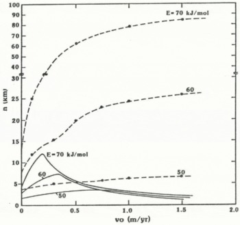
Fig. 4. The critical height hc (solid curves) and the total height (dashed curves) needed to produce fast instabilities as a function of accumulation rate. The criterion for fast instabilities is that tgr (t = 1000 year) = 103 year. The initial thickness is 0.95hc. Other parameters are the same as in Figure 3.
Figure 4 also shows the total height h 0 + Δh (dashed curves) needed to produce a growth time of 1000 years after a time of 1000 years has elapsed following the initial perturbation (h 0 = 0.95h c). The magnitude of Δh needed to trigger such a rapid instability generally increases with it also increases dramatically with E *. When |v 0| exceeds 0.5 m a-1, the necessary Δh at E * = 70 kJ mol-1 is more than 30 times larger than Δh required for E * = 50 kJ mol-1. Ice-thickness perturbations of only a couple of kilometers are adequate to induce fast instabilities when E * = 50 kJ mol-1.
3.3. Time for melting: effects of varying rheological and physical parameters
A more physically meaningful measure of the time-scale for creep instability is the time tm for the basal temperature to reach the solidus temperature of ice. The rheology we have employed is not uniformly valid up to the melting temperature, since the activation energy above -10°C is about twice its value below -10°C on account of significant amounts of recrystallization and grain growth (Reference WeertmanWeertman, 1983). However, this is of little consequence, for once the runaway process has ensued there is very little difference between the time it takes to reach -10°C or 0° C (Fig. 2).
The time to melt is shown in Figure 5 as a function of Δh for various activation energies. The rest of the physical and rheological parameters are taken from the beginning of this paper. Figure 5 also includes a curve associated with no shear heating in the energy equation. Solid curves with shear heating correspond to states with an initial height h 0 of 2 km, while the dashed curves are associated with a smaller h 0 of 1.4 km. In all cases, viscous heating serves to decrease t m relative to the case of no frictional heating. Basal melting requires a minimum of about 2 – 105 year to occur when viscous dissipation is not taken into account. However, with frictional heating, t m can be much less than 2 – 105 year. For t m to be less than 104 year, Δh must be at least 30 km for E * = 70 kJ mol-1, at least 8 km for E * = 60 kJ mol-1, but only 2 km for E * = 50 kJ mol-1. By comparing the solid and dashed curves for E * = 50 kJ mol-1 and noting that the critical height h c for E * = 50 kJ mol-1 is 2.2 km, we can conclude that the instability is faster the closer the initial thickness is to the critical thickness. Ice-thickness perturbations of 1-2 km are capable of producing melting within 104 year for E * less than about 50 kJ mol-1.

Fig. 5. Time for basal melting as a function of the perturbation ice thickness. Solid curves are for h0 = 2 km. while dashed curves represent h0 = 1.4 km. No shear heating means that Equation (2) is solved without the frictional heating term present. Other parameters are the same as in Figure 4.
Effects on t m due to variations in A, v 0, and T s are summarized in Figure 6; in all the cases E * = 60 kJ mol-1. Decreases in A and increases in |v 0| stabilize the ice sheet by increasing t m. An increase in A by a factor of 100 {A = 100A0; A 0 is the nominal value of A given at the beginning of this paper) can lead to fast instabilities for reasonable values of Δh. (Because the critical height h c for the case of 102 A 0 and T s = 235 k is less than 2 km (h c = 1.84 km), we took h 0 in this case to be 1.4 km. For all the solid curves in Figure 6, h 0 = 2 km. For the case T s = 223 K and 10 2 A 0, h c is about 2.3 km.) A comparison of the two cases with different T s but with the same large value of A=102 A 0 shows that an increase in the surface temperature of 12 K can reducet m by a factor of 5 for Δh = 2 km. In general, fast instabilities can be optimized by havaing low values of E *, high values of T s, and large values of A. When all of these ingredients act in concert, then t m approaching 103 year is quite feasible for Δh between 1 and 2 km.

Fig. 6. Melting time as a function of the increase in ice thickness. Solid curves represent initial conditions with h0 = 2.0 km. while dashed curves are associated with h0 = 1.4 km. An activation energy of E* = 60 kJ mol-1 has been employed throughout. Unless otherwise noted in the figure, the other parameters are kept fixed according to the text. The critical heights hc for the cases ( 102A0. ![]() = 223 K) and (102A0.
= 223 K) and (102A0. ![]() = 235 K) are respectively 2.4 and 1.8 km.
= 235 K) are respectively 2.4 and 1.8 km.
The way surface temperature influences the instability is explored in greater detail in Figure 7 which shows h cr and the total ice thickness 0.95h c + Δh necessary to yield a growth time of 103 year after an elapsed time of 103 year, both as functions of T s. Other rheological and physical parameters are taken from the beginning of this paper. Critical ice thickness increases as the environment becomes colder; h c increases by about a factor of two when T s decreases from 240 to 210 K. The magnitude of the ice-thickness perturbation necessary to give t gr (103 year) = 103 year also increases with decreases in T s; the Δh required to induce instabilities with the same rapid time-scale doubles when T s is reduced from 240 to 210 K.

Fig. 7. The critical height and the total height needed for fast instabilities (as defined in the caption to Figure 4) as functions of the surface temperature Ts Parameters are taken from the text.
4. Summary and Concluding Remarks
The overall size and internal state of a polar ice sheet have important influences upon our climate system. Of particular significance for the dynamics and stability of an ice sheet is the state of the basal ice (melted or frozen) beneath most of the “grounded” area. Reference Veen and OerlemansVan der Veen and Oerlemans (1984) have shown that the presence of basal melt water can produce a bifurcation in the steady-state solutions for a polar ice sheet. Two different regimes are possible - a fast flow with a high basal temperature and a slow flow with a low basal temperature.
Our work has addressed the feasibility of inducing massive basal melting by explosive shear-heating instability. We have concentrated on obtaining quantitative estimates of the time-scale of this instability and in so doing have imposed finite-amplitude perturbations in the form of thickened ice layers. The particular form of this perturbation was chosen only for its simplicity. Other perhaps more climatically realistic perturbations can also trigger shear-heating instability. For example, we have conducted calculations to show how climatic warming can also lead to massive basal melting by this frictional heating mechanism.
We have demonstrated that creep instabilities can indeed cause melting of the basal ice layer under circumstances for which the ice would not melt without viscous dissipation. More importantly, we have found that the time-scale for melting can be greatly reduced by shear heating even if basal melting would be the long-term fate of a thickened ice sheet without viscous dissipation. Shear-heating instability has been seen to occur in an explosive manner after the thickened ice sheet simmers for what might be a prolonged period of time. Rapid times for the onset of explosion are strongly favored by low activation energies and large values of the pre-exponential factor in the flow law; i.e. fast instabilities are favored by more ductile creep behavior of ice. Short time-scales for melting by shear-heating instability are also induced by low accumulation rates and high surface temperatures.
Our numerical experiments have shown that shearheating instabilities with fast time-scales of 0(102–103 year) can only be induced in ice sheets by additions of 1–2 km of ice for realistic values of environmental and ice-rheological parameters. Admittedly, the required perturbations are large, when viewed with the thickness of the present Antarctic ice sheet. While the perturbations are prescribed, without consideration of ice thinning (Reference Fowler and LarsonFowler and Larson, 1980), our calculations place a lower bound on the time-scale associated with the non-linear evolution of creep instability, which is much shorter than the linear estimates. The time-scales derived here are also relevant to other types of climatic perturbations, such as long-term warming of the ice surface.
Acknowledgement
This research has been supported by U.S. National Science Foundation grant DPP 8215015.


