


1. Introduction
This paper describes a numerical bifurcation analysis of unconfined, incompressible swirling jets. Even in the laminar regime, swirling jets host a suite of rich physics due to the complex interplay among axial and azimuthal shear layers, centrifugal instabilities and propagating inertial waves. Although scientifically interesting in their own right, these flows are of crucial importance to the engineering of various modern technologies including gas turbine combustors, cyclonic separators and aeronautical lift and control surfaces. Swirling jets are also a core feature of numerous natural flows including tornadoes, cyclones and quasars. At a more fundamental level, even turbulent eddies in general are affected by many of the same phenomena as swirling jets, such as vortex breakdown.
Despite their significance, obtaining detailed and repeatable characterisations of the swirling jet parameter space via experiments or conventional time-marching computations remains challenging. This is due partly to the sheer variety of different flow patterns that have been reported across the literature, but also to the multistability and hysteresis which can relate distinct states. Without a deeper understanding of the overall parameter space, any observation must be taken in the specific context of the flow configuration, including the initial conditions, confinement, external noise sources and geometrical variations. There is a need for a more comprehensive ‘taxonomy’ of swirl flow configurations and dynamics in order to relate different studies by a more general set of behaviours. This observation serves as a key motivation for this work, with our focus here being on unconfined, fully developed laminar swirling jets.
As suggested above, one of the most salient features of swirling flows is the phenomenon of vortex breakdown. Vortex breakdown occurs when the axial flow along or near the vortex axis abruptly stagnates beyond a certain level of swirl. In most swirling flow configurations, this phenomenon is associated with exchanges of stability and multistability among various axisymmetric and spiral states (Leibovich Reference Leibovich1984; Ash & Khorrami Reference Ash and Khorrami1995). A classic early example is Lambourne & Bryer's (Reference Lambourne and Bryer1962) famous photograph of the flow over a delta wing exhibiting simultaneous ‘spiral’ and ‘bubble’ breakdown patterns. Throughout the literature of swirling flows, significant effort has been exerted to categorise the observed forms of vortex breakdown into relatively few canonical types.
In the inviscid limit, columnar swirling flows (i.e. axisymmetric rotating flows with bulk axial motion and zero radial velocity) are subject to three fundamental instability mechanisms which generally interact to control the overall stability behaviour. First is centrifugal instability which occurs due to a local imbalance between the centrifugal force and the radial pressure gradient. In the linear limit, asymptotic analyses have shown that this mechanism tends to most strongly amplify helical modes with wavenumber vectors that are oriented along the direction of zero strain of the bulk flow (Leibovich & Stewartson Reference Leibovich and Stewartson1983; Billant & Gallaire Reference Billant and Gallaire2013). Next, the Kelvin–Helmholtz instability arises in swirling jets due to both the axial and azimuthal components of velocity shear. Under the so-called ‘tilting shear’ approximation (which neglects curvature effects) it has been shown that the linear shear mechanism in swirling flows tends to selectively amplify helical disturbances with a wavenumber vector parallel to the direction of maximal strain of the bulk flow (Martin & Meiburg Reference Martin and Meiburg1994; Gallaire & Chomaz Reference Gallaire and Chomaz2003a). Finally, the stability of columnar swirling jets is influenced by the Coriolis effect, giving rise to travelling inertial waves (Kelvin Reference Kelvin1880). As originally suggested by Squire (Reference Squire1960) and Benjamin (Reference Benjamin1962) and later clarified by Wang & Rusak (Reference Wang and Rusak1997) and Wang et al. (Reference Wang, Rusak, Gong and Liu2016), this Coriolis mechanism is closely related to the nonlinear phenomenon of vortex breakdown, although the overall vortex breakdown process is more delicate in flow situations where the shear and centrifugal mechanisms are also active.
This study is directed towards laminar swirling jets exhausting into open environments, where viscosity and geometry, in addition to generating their own new physics, prohibit any clean separation of the basic mechanisms discussed above. The first efforts to understand such flows appeared in the 1960s and were primarily motivated by engineering applications in swirl-stabilised combustion. Early studies of swirling jets (Chigier & Chervinsky Reference Chigier and Chervinsky1967) focused heavily on developing empirical correlations for the macroscopic flow characteristics based on measured turbulence statistics. Although controlled fundamental experiments were commonplace at the time in confined swirling flows such as vortex tubes (Harvey Reference Harvey1962; Sarpkaya Reference Sarpkaya1971) and rotating cylinders (Vogel Reference Vogel1968), it was not until over two decades later that studies began to investigate the physical processes underlying these statistics in unconfined swirling jets. For example, influential work by Farokhi, Taghavi & Rice (Reference Farokhi, Taghavi and Rice1989) highlighted the effect of swirl and forcing distribution (and not just magnitude) on the flow characteristics. Other authors such as Panda & McLaughlin (Reference Panda and McLaughlin1994) and Martin & Meiburg (Reference Martin and Meiburg1996) expanded on these ideas, advancing a dynamical systems perspective toward the behaviour of swirling jets which emphasised the role of coherent vortical structures and instabilities over turbulence statistics. Such ideas are the basis of most recent studies of turbulent swirling jet dynamics (Oberleithner et al. Reference Oberleithner, Sieber, Nayeri, Paschereit, Petz, Hege, Noack and Wygnanski2011; Tammisola & Juniper Reference Tammisola and Juniper2016; Manoharan et al. Reference Manoharan, Frederick, Clees, O'Connor and Hemchandra2020); however, our study is exclusively focused on swirling jets at much lower Reynolds numbers.
Within this modern paradigm, the LadHyX group performed a series of experiments examining the dynamics of transitional water jets discharging from a rotating pipe into a large tank. Beginning with the study by Billant, Chomaz & Huerre (Reference Billant, Chomaz and Huerre1998), they systematically explored the vortex breakdown process at various Reynolds numbers as a function of the swirl ratio. A key contribution of this research was the description of the ‘cone’ form of vortex breakdown and the bistable relationship between it and the more well-known ‘bubble’ form over a certain range of swirl and Reynolds numbers. Time-domain simulations have corroborated this interpretation of the cone and bubble as bistable breakdown states in swirling jets (Ogus, Baelmans & Vanierschot Reference Ogus, Baelmans and Vanierschot2016; Moise Reference Moise2020), but the relationship between these states has not yet been clearly shown. This dynamics will be explicitly demonstrated in this paper through numerical continuation of the relevant solution branches.
Another feature of the LadHyX experiments was the use of planar flow visualisation techniques along multiple measurement planes. These methods were used by Billant et al. (Reference Billant, Chomaz and Huerre1998) to provide a clearer perspective of the jet's three-dimensional dynamics compared to earlier line-of-sight observations. In particular, their visualisations detailed a spiral flow structure of azimuthal periodicity  $|m|=2$ which rotated in time in the same direction as the imposed rotation. This instability appeared at swirl ratios well below those associated with the formation of any central stagnation point and diminished at higher levels of swirl as either cone or bubble-type breakdown appeared. In certain conditions after breakdown, the flow was dominated by asymmetric,
  $|m|=1$, spiral structures. Note that, throughout the range of swirl ratios examined by Billant et al. (Reference Billant, Chomaz and Huerre1998), unsteady ‘Kelvin–Helmholtz-like billows’ were also present, although these structures were not a major focus of that study.
In a later study using the same experimental apparatus, Loiseleux & Chomaz (Reference Loiseleux and Chomaz2003) focused more specifically on the system's behaviour before vortex breakdown. They described three distinct pre-breakdown regimes where a variety of unsteady axisymmetric and spiral structures exchange dominance with varying swirl. In the non-swirling case, the shear layer rolled up into nominally axisymmetric ring structures due to the Kelvin–Helmholtz instability. In the first regime, at low swirl ratios, co-rotating spiral structures began to appear over the primary axisymmetric vortex rings, presumably due to secondary instability. The azimuthal periodicity of these spiral structures gradually decreased from  $|m|=7$ to
  $|m|=5$ with increasing swirl until reaching a transitional stage where axisymmetric ring structures again prevailed. In the second regime, the co-rotating
  $|m|=2$ spiral instability reported by Billant et al. (Reference Billant, Chomaz and Huerre1998) strongly dominated the flow dynamics, eliminating any distinction between primary vs secondary instability. Finally, in the third regime immediately preceding vortex breakdown, a distinct counter-rotating motion with
  $|m|=1$ periodicity appeared in addition to other intermittent axisymmetric and three-dimensional structures of similar amplitude.
Similar experimental descriptions of deterministic flow structures in swirling jets have also been detailed by Liang & Maxworthy (Reference Liang and Maxworthy2005, Reference Liang and Maxworthy2008). Their observations agree qualitatively with the earlier studies by the LadHyX group, while providing more quantitative insight into the dynamics thanks to improved velocimetry techniques. In particular, spectral analysis suggested that the axisymmetric oscillations emphasised by Gallaire & Chomaz (Reference Gallaire and Chomaz2003b) are primarily excited by external noise, suggesting a passive amplifier role for the  $m=0$ pulsations associated with convective instability. In contrast, they argued that the pre-breakdown
  $|m|=2$ and post-breakdown
  $|m|=1$ instabilities also reported by Billant et al. (Reference Billant, Chomaz and Huerre1998) represent self-excited flow oscillations that are present independent of external noise. This latter point is further supported by the lack of receptivity of swirling jets to
  $|m|=2$ forcing, as observed in the experiments of Gallaire, Rott & Chomaz (Reference Gallaire, Rott and Chomaz2004). Based on their observations, Liang & Maxworthy (Reference Liang and Maxworthy2005) further characterised the bifurcations underlying the self-excited instabilities by fitting their measured oscillation amplitude–swirl ratio relationship to an unforced supercritical Landau equation model. Despite a relatively high level of background noise, they found evidence that both instabilities are associated with supercritical Hopf bifurcations and determined approximate critical swirl values for each. The numerical results presented in this paper corroborate the existence of Hopf bifurcations associated with both
  $|m|=2$ and
  $|m|=1$ self-excited oscillations but, significantly, also show the presence of subcritical bifurcations. Ruith et al. (Reference Ruith, Chen, Meiburg and Maxworthy2003) performed a comprehensive numerical investigation of unconfined swirling flow using the Grabowski & Berger (Reference Grabowski and Berger1976) vortex model. Based on both axisymmetric and three-dimensional unsteady simulations, Ruith et al. (Reference Ruith, Chen, Meiburg and Maxworthy2003) systematically surveyed the parameter space and noted the emergence of steady, axisymmetric vortex breakdown and its eventual instability toward spiralling vortical structures associated with either
  $|m|=2$ or
  $|m|=1$. Thanks to their detailed study, the Grabowski–Berger vortex has become a standard flow for analysis of swirling flow dynamics, attracting significant theoretical attention over the previous decade (Gallaire et al. Reference Gallaire, Ruith, Meiburg, Chomaz and Huerre2006; Vyazmina et al. Reference Vyazmina, Nichols, Chomaz and Schmid2009; Meliga, Gallaire & Chomaz Reference Meliga, Gallaire and Chomaz2012; Qadri, Mistry & Juniper Reference Qadri, Mistry and Juniper2013; Pasche, Avellan & Gallaire Reference Pasche, Avellan and Gallaire2018). However, it is also important to note that this model vortex does not capture all aspects of the flows found in a broad class of physically interesting swirling jet applications. For instance, the Grabowski–Berger vortex is defined by a fixed parallel inflow condition which exhibits substantial axial co-flow over the entire radial extent of the domain. Swirling jets, in contrast, are typically surrounded by nominally quiescent surroundings. As a result of key differences like this, the relationship between the dynamics of the Grabowski–Berger vortex model and those of many swirling jets realised in the laboratory or in practical hardware is unclear. This paper will highlight some important commonalities and distinctions between their behaviours.
Recently, Moise & Mathew (Reference Moise and Mathew2019) performed nonlinear simulations of a different fixed vortex model which is more representative of this broader class of swirling jets. They documented a variety of characteristic flow states and, as expanded upon in a subsequent paper (Moise Reference Moise2020), described hysteresis with respect to swirl among these states. As mentioned above, their simulations are some of the first to demonstrate hysteresis between bubble and cone-type vortex breakdown topologies. Their results also reproduced some of the experimentally observed  $|m|=1$ and
  $|m|=2$ spiral structures from Billant et al. (Reference Billant, Chomaz and Huerre1998) and Liang & Maxworthy (Reference Liang and Maxworthy2005), in addition to several new flow features. However, their time-domain solution approach did not support a detailed bifurcation analysis like the one we will pursue here.
In summary, many key elements of unconfined laminar swirling jets dynamics have been identified. Both experiments and simulations have described a variety of coherent flow patterns and documented multistability among the different flow states. Theories have also been developed to explain, under specific conditions, the basic physical mechanisms which interact in more general situations to express the observed features. Yet, this body of existing knowledge still requires a consistent, comprehensive framework for comparison, generalisation and interpretation. The main contribution of this study is a series of bifurcation analyses which unambiguously characterise the nonlinear dynamics of steady and time-periodic solutions in an unconfined swirling jet configuration with a fully developed inflow profile. This provides insight into the topology of the underlying parameter space, which, in turn, enables a deeper and more general understanding of the physics controlling swirling jet behaviour.
The rest of this article is organised as follows. Section 2 details our flow configuration by defining the geometry, the continuous governing equations and the boundary conditions. Section 3 describes the numerical methods, including the weak formulation, the finite element discretisation and the numerical algorithms used to obtain the results. Section 4 presents our results regarding the steady, axisymmetric flow states in swirling jets and characterises the stability of these solutions with respect to three-dimensional and unsteady behaviour. In § 5, we turn our attention to periodic solutions and examine the dynamics of nonlinear limit cycles associated with the instabilities identified in § 4. Finally, § 6 presents a summary of our results in the context of existing literature and suggests directions for future research.
2. Flow configuration
We consider viscous, constant-density swirling jets discharging from a long, straight, rotating pipe into a semi-infinite domain as depicted in figure 1. Conventional cylindrical-polar coordinates defined by  $\boldsymbol {x}=(x,r,\theta )$ are adopted with the origin located at the centre of the pipe exit. All quantities are dimensionless; the lengths being normalised by the pipe diameter
  $D=2R$ and the velocities by the steady, volume-averaged flow velocity
  $U$ through the pipe. Consequently, the two independent parameters governing this flow are the swirl ratio
  $S=\omega R/U$ and the Reynolds number
  $\textit {Re}=DU/\nu$ where
  $\omega$ is the rotation rate of the pipe and
  $\nu$ is the fluid's kinematic viscosity. The fluid motion is described by the velocity
 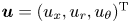 $\boldsymbol {u}=(u_x,u_r,u_\theta )^{\mathrm {T}}$ and pressure
  $p$ fields, which together evolve in the domain according to the incompressible Navier–Stokes and continuity equations,
 \begin{gather} \frac{\partial\boldsymbol{u}}{\partial t}+\boldsymbol{u}\boldsymbol{\cdot}\boldsymbol{\nabla}\boldsymbol{u}={-}\boldsymbol{\nabla} p+\frac{1}{\textit{Re}}\nabla^{2}\boldsymbol{u}, \end{gather}
 \begin{gather}0= \boldsymbol{\nabla}\boldsymbol{\cdot}\boldsymbol{u}. \end{gather}
Figure 1. Schematic of the meridional plane of the axisymmetric domain  $\varOmega$ with boundary
  $\varGamma$.
The swirling jet configuration we have selected has some important distinctions from the experimental set-ups used at LadHyX (Billant et al. Reference Billant, Chomaz and Huerre1998) or by Liang & Maxworthy (Reference Liang and Maxworthy2005, Reference Liang and Maxworthy2008). First, unlike the top hat-like jet profiles seen in these experimental studies, our jet issues from the pipe with a fully developed velocity profile. This choice conveniently eliminates any significant dependence of the jet's velocity profile on the length of the inlet pipe and the Reynolds number. Second, in order to simplify the geometry, we have placed the reservoir wall flush with the pipe exit and included far-field boundary conditions which simulate an unconfined jet. Conversely, the experimental studies cited above have injected the jet some distance past the containing wall into a closed tank with a lateral and axial extent of the order of ten times the jet diameter.
A complete listing of the boundary conditions associated with (2.1) are given in . Axial flow is controlled by a prescribed steady mass flux through the pipe, and no-slip conditions are enforced for all velocity components on the rotating pipe wall  $\varGamma _p$ and the fixed exit-plane wall
  $\varGamma _w$. Conceptually, the inlet pipe is sufficiently long such that a region exists where the flow is fully developed but exit effects are negligible. The upstream boundary
  $\varGamma _i$ is located at some
  $x=-\ell$ in this region where the distribution of axial and azimuthal velocity is fixed to match the Poiseuille solution. Note that instead of rigidly enforcing a parallel inflow at
  $\varGamma _i$, less-restrictive Neumann conditions are enforced on the radial component of velocity to minimise inlet reflections and scattering of upstream-propagating vorticity disturbances and inertial waves (Rusak Reference Rusak1998). On the central axis
  $\varGamma _{a}$, three-dimensional symmetry constraints based on a Fourier expansion along
  $\theta$ are derived from parity considerations for each velocity component in the limit of
  $r\rightarrow 0$ for each azimuthal wavenumber
  $m$ (Boyd Reference Boyd2013). The jet exits the pipe into a semi-infinite, quiescent reservoir which is truncated to the large but finite radius
  $R_\infty$ for practical purposes. The nominal configuration used for this paper is specified by the values
  $\ell =4$ and
  $R_\infty =40$ which were selected on the basis of a parameter sensitivity analysis presented in Appendix A. However, as will be discussed later, many calculations were repeated on meshes with higher
  $\ell$ and
  $R_\infty$ values in order to ensure grid independence.
Table 1. List of boundary conditions.

To accurately model the unconfined flow, transparent constraints along the open boundary  $\varGamma _o$ are required. As emphasised by Ruith, Chen & Meiburg (Reference Ruith, Chen and Meiburg2004) and Vyazmina et al. (Reference Vyazmina, Nichols, Chomaz and Schmid2009), such conditions must not only allow flow to passively exit the domain without generating wave reflection artefacts but must also enable free entrainment from the far field. A constraint which satisfies both of these requirements in non-swirling flows and emerges naturally in the variational formulation of (2.1) is the well-known free-outflow condition given by
 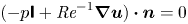 $(-p{\boldsymbol{\mathsf{I}}}+\textit {Re}^{-1}\boldsymbol {\nabla }\boldsymbol {u})\boldsymbol {\cdot }\boldsymbol {n}=0$, where
  ${\boldsymbol{\mathsf{I}}}$ is the identity matrix and
  $\boldsymbol {n}$ is the outward unit normal vector. However, this condition raises two major concerns for the strongly swirling and recirculating flows considered here. First, the free-outflow condition requires the normal derivative of the normal flow component to exactly balance the pressure along the boundary. In a scenario where centrifugal effects due to swirl induce a physical variation in pressure along the open boundary, the free-outflow condition will generate non-physical flow gradients to match this variation. Second, when there is inward flow across the boundary, the free-outflow condition does not restrict the energy entering the domain and may lead to ill-posedness.
To mitigate these problems, other studies employing free-outflow conditions for investigations of open swirling flows have employed extended computational domains with artificial sponge layers. This approach seeks to avoid the aforementioned concerns by using large amounts of artificial dissipation to rapidly develop the flow to a purely outward Poiseuille form with negligible azimuthal velocity before it reaches the outflow boundary. While effective, such treatment adds design challenges and computational expenses associated with the parameters of the sponge layer and the increased domain size. We have taken a different approach. The boundary stress issue is avoided by excluding the centrifugal pressure variations from the normal stress balance on the boundary, while ill-posedness is avoided using a robust directional outflow condition which remains well-posed even with substantial entrainment from the domain exterior. To decouple the centrifugal pressure from the outflow boundary condition, we proceed by defining the modified pressure  $\tilde {p}=p-p_o$ along the open boundary. Here,
  $p_o$ is a scalar potential which characterises the centrifugal pressure variations along
  $\varGamma _o$ via the relation
 \begin{equation} \boldsymbol{\nabla} p_o\boldsymbol{\cdot}\boldsymbol{t}=\left.\frac{u_\theta^{2}}{r}\right|_{\varGamma_o}, \end{equation}
where  $\boldsymbol {t}$ is the positively oriented unit tangent vector along
  $\varGamma _o$. Since (2.1c) only defines
  $p_o$ up to a constant, we take
  $p_o=0$ at
  $\varGamma _w\cap \varGamma _o$ for uniqueness. Then, saving the details for the next section,
  $p_o$ is excluded from the pressure term in the open boundary condition so that centrifugal pressure variations are decoupled from the flow gradients on the boundary.
Next, to address the issue of recirculating flow from the domain exterior, we adopt the directional outflow condition  $(-p{\boldsymbol{\mathsf{I}}}+\textit {Re}^{-1}\boldsymbol {\nabla }\boldsymbol {u})\boldsymbol {\cdot }\boldsymbol {n}- \frac {1}{2}\boldsymbol {u}\min (0,\boldsymbol {u}\boldsymbol {\cdot }\boldsymbol {n})=0$, following Bruneau & Fabrie (Reference Bruneau and Fabrie1994). This condition, reviewed recently by Bertoglio et al. (Reference Bertoglio, Caiazzo, Bazilevs, Braack, Esmaily, Gravemeier, Marsden, Pironneau, Vignon-Clementel and Wall2018), is identical to the conventional Neumann-type free-outflow condition along any part of the open boundary with a local outflow, but exhibits dissipation related to the weak form of the advection term wherever back flow (i.e.
  $\boldsymbol {u}\boldsymbol {\cdot }\boldsymbol {n}<0$) occurs. This yields a stable Robin-type condition which bounds the energy influx and promotes well-posedness while still respecting the important exchange of mass and momentum across the open boundary (Braack & Mucha Reference Braack and Mucha2014).
Combining the directional outflow condition with the centrifugal pressure decoupling approach yields the modified directional outflow boundary condition given in . This condition is applied along the entirety of the open boundary  $\varGamma _o$. In the absence of swirl, this constraint reduces exactly to the directional outflow condition and further to the free-outflow condition if the flow is also purely outward across
  $\varGamma _o$.
3. Problem formulation
3.1. Numerical method
Our numerical methods are derived from the variational form of (2.1) and the boundary conditions of including (2.1c). To remove the coordinate singularity at  $r=0$, (2.1a) is first multiplied by the radial coordinate (Meliga & Gallaire Reference Meliga and Gallaire2011). Then, taking the standard real or complex
  $L^{2}$ inner product
  $\langle \bullet ,\bullet \rangle _\varOmega$ and introducing test functions
 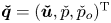 $\boldsymbol {\check {q}}=(\boldsymbol {\check {u}},\check {p},\check {p}_o)^{\mathrm {T}}$, we integrate over the domain, seeking in the appropriate spaces
  $\boldsymbol {q}=(\boldsymbol {u},p,p_o)^{\mathrm {T}}$ such that
  $\forall \boldsymbol {\check {q}}$
 \begin{align} &\left\langle r\boldsymbol{\check{u}},\frac{\partial\boldsymbol{u}}{\partial t} +\boldsymbol{u}\boldsymbol{\cdot}\boldsymbol{\nabla}\boldsymbol{u}\right\rangle_{\varOmega} +\left\langle\boldsymbol{\nabla}(r\boldsymbol{\check{u}}),-p{\boldsymbol{\mathsf{I}}} +\frac{1}{\textit{Re}}\boldsymbol{\nabla}\boldsymbol{u}\right\rangle_{\varOmega} +\langle \check{p},\boldsymbol{\nabla}\boldsymbol{\cdot}\boldsymbol{u}\rangle_{\varOmega}\nonumber\\ &\quad +\left\langle r\boldsymbol{\check{u}},p_o\boldsymbol{n}- \frac{1}{2}\boldsymbol{u}\min(0,\boldsymbol{u}\boldsymbol{\cdot}\boldsymbol{n}) \right\rangle_{\varGamma_o}+\left\langle \check{p}_o,\boldsymbol{\nabla} p_o\boldsymbol{\cdot} \boldsymbol{t}-\frac{u_\theta^{2}}{r}\right\rangle_{\varGamma_o}=0. \end{align}
Note that weak form of the modified directional outflow condition described above results in a boundary integral along  $\varGamma _o$ which is simplified by the application of the divergence theorem to the viscous and pressure terms of (2.1).
The spatial discretisation consists of a Delaunay triangulation of the meridional plane constructed using GMSH (Geuzaine & Remacle Reference Geuzaine and Remacle2009). After experimentation with several different meshes, we selected a primary triangulation for  $\varOmega$ with
  $\ell =4$ and
  $R_\infty =40$ which features
  $140\ 055$ elements, although many key calculations were also repeated on larger meshes to ensure mesh convergence. Finally, an inf-sup stable discrete problem is formed by projecting the weak formulation of (3.1) onto the basis of Taylor–Hood
  $(\mathbb {P}_2\times \mathbb {P}_1)$ finite elements associated with the mesh using FreeFEM (Hecht Reference Hecht2012). The velocity
  $\boldsymbol {u}$ and pressure
  $p$ are defined respectively on bi-quadratic and bi-linear elements over the full domain
  $\varOmega$, while the centrifugal pressure
  $p_o$ is defined on linear elements along only the boundary
  $\varGamma _o$. The resulting discrete flow states have
  $915\ 839$ total degrees of freedom on the primary mesh. Further details of the mesh and an assessment of the robustness of our results to the selected discretisation are provided in Appendix A.
3.2. Solution methodologies
Although our actual implementation is based on the weak form of the autonomous nonlinear system (3.1), for convenience of notation, further discussion will make use of the strong state-space form,
 \begin{equation} {\boldsymbol{\mathsf{M}}}\frac{\partial\boldsymbol{q}}{\partial t}+\mathcal{R} (\boldsymbol{q};\textit{Re},S)=0, \end{equation}
where  $\textit {Re}$ and
  $S$ are parameters and the strong forms of the mass matrix and steady Navier–Stokes operators are, respectively,
 \begin{equation} {\boldsymbol{\mathsf{M}}}=\begin{pmatrix} {\boldsymbol{\mathsf{I}}} & 0 & 0\\0 & 0 & 0\\0 & 0 & 0\end{pmatrix}\quad \mbox{and} \quad\mathcal{R}(\boldsymbol{q})=\begin{pmatrix} \boldsymbol{u}\boldsymbol{\cdot}\boldsymbol{\nabla}\boldsymbol{u}+\boldsymbol{\nabla} p-\dfrac{1}{\textit{Re}}\nabla^{2}\boldsymbol{u}\\ \boldsymbol{\nabla}\boldsymbol{\cdot}\boldsymbol{u}\\ \boldsymbol{\nabla} p_o\boldsymbol{\cdot}\boldsymbol{t}-\dfrac{u_\theta^{2}}{r} \end{pmatrix}. \end{equation}
This notation neglects several important aspects of the weak form, including the boundary conditions and the restriction of (2.1c) to  $\varGamma _o$. In our parallel implementation, all problems are abstracted to the linear algebra level by FreeFEM (Hecht Reference Hecht2012; Moulin, Jolivet & Marquet Reference Moulin, Jolivet and Marquet2019) and solved in a distributed manner using PETSc (Balay et al. Reference Balay2020) based on direct factorisation via MUMPS (Amestoy et al. Reference Amestoy, Duff, Koster and L'Excellent2001) except where noted otherwise.
3.2.1. Identification and continuation of equilibrium states
Since the geometry and boundary conditions are independent of  $\theta$ and
  $t$, the steady states
  $\boldsymbol {q}_0(x,r)$ of this flow represent axisymmetric fixed points of (3.2). Such solutions are commonly termed ‘base flows’ or ‘steady states’ in the stability literature; we will refer to them as the latter in this paper. Hence,
  $\boldsymbol {q}_0$ is defined as an equilibrium satisfying
 \begin{equation} \mathcal{R}_{0}(\boldsymbol{q}_0;\textit{Re},S)=0, \end{equation}
where the 0-subscript on  $\mathcal {R}_0$ is used to indicate a restriction of the steady three-dimensional operator
  $\mathcal {R}$ to its axisymmetric Fourier component. A similar
  $m$-subscript convention is used throughout this paper to indicate the restriction of any three-dimensional operator to the
  $m$th component of its azimuthal Fourier decomposition by formally replacing any partial derivatives along
  $\theta$ with the product
  $\mathrm {i}m$.
One simple strategy to find  $\boldsymbol {q}_0$ is by locking the values of all parameters and using Newton's method to iteratively refine an initial guess for the steady flow. In this approach, the correction
  $\delta \boldsymbol {q}_0$ to the initial guess
  $\boldsymbol {q}_0$ is then determined by solving the linear problem,
 \begin{equation} {\boldsymbol{\mathsf{J}}}_{0}(\boldsymbol{q}_0)\delta\boldsymbol{q}_0=\mathcal{R}_0(\boldsymbol{q}_0), \end{equation}
where the action of the Jacobian matrix is
 \begin{equation} {\boldsymbol{\mathsf{J}}}_{m}(\boldsymbol{q}_0)\delta\boldsymbol{q}_m=\begin{pmatrix} \boldsymbol{u}_0\boldsymbol{\cdot}\boldsymbol{\nabla}_m({\bullet})+({\bullet})\boldsymbol{\cdot} \boldsymbol{\nabla}_0\boldsymbol{u}_0-\dfrac{1}{\textit{Re}}\nabla_m^{2}({\bullet}) & \boldsymbol{\nabla}_m({\bullet}) & 0\\ \boldsymbol{\nabla}_m\boldsymbol{\cdot}({\bullet}) & 0 & 0\\ -\dfrac{2u_{\theta,0}}{r}({\bullet})\boldsymbol{\cdot}\boldsymbol{e}_\theta & 0 & \boldsymbol{\nabla}_m({\bullet})\boldsymbol{\cdot}\boldsymbol{t} \end{pmatrix}\begin{pmatrix} \delta\boldsymbol{u}\\\delta p\\\delta p_o \end{pmatrix}_m, \end{equation}
and  $\boldsymbol {e}_\theta$ refers to a unit vector along
  $\theta$. Following each iteration, the state is updated as
  $\boldsymbol {q}_0\leftarrow \boldsymbol {q}_0-\delta \boldsymbol {q}_0$, and the process is repeated until the norm of the residual converges within
  $\|\mathcal {R}_0\|<10^{-10}$.
While sufficient for such purposes as initialising a solution branch, the straightforward approach outlined above is not always robust for continuation of a branch along a parameter. In general, nonlinear systems may exhibit multiple solutions at identical parameter values, and the domain of convergence for Newton's method shrinks as the Jacobian matrix becomes singular near a bifurcation point. A more suitable approach for such systems involves tracing branches of  $\boldsymbol {q}_0$ using a predictor–corrector scheme which can ‘jump’ over singularities (Keller Reference Keller1978). Methods of this type treat both the state vector
  $\boldsymbol {q}_0$ and a continuation parameter
  $\alpha$ (here either
  $S$ or
  $\textit {Re}$) as unknowns in (3.4), and require an additional constraint to compensate for this new degree of freedom.
Our continuation approach relies on a predictor–corrector scheme with a tangent predictor step and a Moore–Penrose corrector sequence. For the predictor step, we exploit the fact that the null vector associated with the augmented Jacobian matrix at a point on the solution curve lies tangent to the solution curve at that point. More precisely, the null vector  $\boldsymbol {y}=(\boldsymbol {y}_{\boldsymbol {q}},y_\alpha )^{\mathrm {T}}$ satisfies
 \begin{equation} \boldsymbol{y}\in\ker\left(\left[{\boldsymbol{\mathsf{J}}}_{0}(\boldsymbol{q}_0,\alpha), \frac{\partial\mathcal{R}_0(\boldsymbol{q}_0,\alpha)}{\partial\alpha}\right]\right), \end{equation}
where the vector  $\partial \mathcal {R}_0/\partial \alpha$ is approximated via finite differences. To determine
  $\boldsymbol {y}$ and fix its orientation with respect to the parameter, we set
  $y_\alpha =-1$ and solve
 \begin{equation} {\boldsymbol{\mathsf{J}}}_{0}(\boldsymbol{q}_0,\alpha) \boldsymbol{y}_{\boldsymbol{q}}=\frac{\partial\mathcal{R}_0 (\boldsymbol{q}_0,\alpha)}{\partial\alpha}. \end{equation}
Thus, a linear prediction for a new point on the solution curve is obtained by taking  $(\boldsymbol {q}_0,\alpha )=(\boldsymbol {q}_0,\alpha ) +h(\boldsymbol {y}_{\boldsymbol {q}},y_\alpha )/\|\boldsymbol {y}\|$, where
  $h$ is a parameter which controls the size and orientation of the predictor step. To enable accurate branch tracing without the expense of needlessly small steps, the magnitude of
  $h$ must be consistently adjusted throughout the continuation process. Our approach uses an adaptive scaling for
  $h$ based on the convergence behaviour of the previous corrector sequence following Allgower & Georg (Reference Allgower and Georg1990) and described below. Furthermore, to ensure a consistent sense of direction along the solution branch, the sign of
  $h$ must be flipped when a saddle-node bifurcation is traversed. We achieve this by monitoring the sign of the inner product between the null vectors associated with each consecutive pair of solution points. When these points lie on either side of a limit point, the inner product is negative and the sign of
  $h$ is reversed.
Following each predictor step, a nonlinear correction sequence is required to converge from the predicted point to a true equilibrium solution  $\boldsymbol {q}_0$. For this we have adopted a Moore–Penrose approach where each Newton iteration of the corrector is constrained to be orthogonal to the kernel of the augmented Jacobian matrix at the current point. Thus, at each iteration, we are faced with the bordered linear system,
 \begin{equation} \begin{pmatrix} {\boldsymbol{\mathsf{J}}}_{0}(\boldsymbol{q}_0,\alpha) & \dfrac{\partial\mathcal{R}_0(\boldsymbol{q}_0,\alpha)}{\partial\alpha}\\ \boldsymbol{y}_{\boldsymbol{q}}^{\mathrm{T}} & y_{\alpha} \end{pmatrix} \begin{pmatrix} {\rm \Delta} \boldsymbol{q}_0\\ {\rm \Delta} \alpha \end{pmatrix} =\begin{pmatrix} \mathcal{R}_0(\boldsymbol{q}_0,\alpha)\\ 0 \end{pmatrix}. \end{equation}
 While (3.9) could be directly assembled and solved at each iteration, this approach is avoided for two reasons. First, since it contains  $\boldsymbol {y}$, the augmented system matrix in (3.9) requires the solution of (3.8) prior to its assembly at each iteration. Second, the presence of the dense vectors
  $\boldsymbol {y}_{\boldsymbol {q}}^{\mathrm {T}}$ and
  ${\boldsymbol{\mathsf{J}}}_\alpha$ on the borders of this augmented system matrix greatly complicate its overall structure in comparison to the sparse Jacobian matrix
  ${\boldsymbol{\mathsf{J}}}_0$ underlying the conventional system in (3.5).
Instead, we have adopted a block elimination strategy to treat (3.9) without explicitly forming the bordered system. We begin by separately solving (3.8) and (3.5). Since these systems involve the same  ${\boldsymbol{\mathsf{J}}}_{0}$, only a single sparse matrix must be assembled and factored to solve both problems. Then, using some algebra based on the Schur complement, the solution to (3.9) is deduced as
 \begin{gather} {\rm \Delta} \alpha= \frac{\boldsymbol{y}_{\boldsymbol{q}}^{\mathrm{T}} \delta\boldsymbol{q}_0}{1+\boldsymbol{y}_{\boldsymbol{q}}^{\mathrm{T}} \boldsymbol{y}_{\boldsymbol{q}}}, \end{gather}
 \begin{gather}{\rm \Delta} \boldsymbol{q}_0= \delta\boldsymbol{q}_0- \boldsymbol{y}_{\boldsymbol{q}} {\rm \Delta} \alpha. \end{gather}
From here, the state is updated as  $(\boldsymbol {q}_0,\alpha )^{\mathrm {T}}\leftarrow (\boldsymbol {q}_0, \alpha )^{\mathrm {T}}-( {\rm \Delta} \boldsymbol {q}_0, {\rm \Delta} \alpha )^{\mathrm {T}}$ and the process is repeated until reaching the same convergence tolerance of
  $\|\mathcal {R}_0\|<10^{-10}$. For further efficiency gains, we treat this corrector sequence as a Newton-chord iteration where a single factorisation of
  ${\boldsymbol{\mathsf{J}}}_{0}$ from the first corrector iteration is reapplied to the remaining iterations until convergence. Once convergence is achieved, the null vector from the last corrector iteration is then reused in the next predictor step.
As indicated above, well-designed adaptive step controls for the predictor are a key aspect of robust continuation methods. Nonetheless, strict convergence conditions are also needed for the corrector to ensure robust and accurate branch tracing. Our requirements include: (i) a monotonic convergence of the residual norm during the corrector iterations, (ii) a decrease in the norm of the correction by at least a factor of two in each iteration, (iii) a norm of the first correction smaller than one, (iv) an angle between consecutive tangent vectors of less than  $30^{\circ }$ and (v) no more than ten corrector iterations per step. If any of these conditions fail to be met during the corrector process before the residual norm reaches the allowed tolerance, the step is rejected, and a new corrector sequence begins from a predictor with half the original step size. Otherwise, the converged step is accepted, and the step size for the next predictor is scaled based on requirements (ii–iv) as described in Allgower & Georg (Reference Allgower and Georg1990).
3.2.2. Stability analysis of steady states
The stability of axisymmetric equilibrium solutions to (3.2) is assessed by the long-time asymptotic evolution of superimposed three-dimensional infinitesimal perturbations  $\boldsymbol {\acute {q}}$ to
  $\boldsymbol {q}_0$. Due to the underlying symmetries of the flow system, any solution to (3.2) can be expanded as a superposition of modes
  $\boldsymbol {\hat {q}}_m$ associated with azimuthal wavenumber
  $m$, growth rate
  $\sigma$ and frequency
  $f$ according to
 \begin{equation} \boldsymbol{\acute{q}}(x,r,\theta,t)\propto \boldsymbol{\hat{q}}_m(x,r)\, \textrm{e}^{\mathrm{i}m\theta+ (\sigma+\mathrm{i}2{\rm \pi} f)t}+\boldsymbol{\hat{q}}_{m}^{*} (x,r)\, \textrm{e}^{-\mathrm{i}m\theta+(\sigma-\mathrm{i}2{\rm \pi} f)t}, \end{equation}
where  $^{*}$ denotes complex conjugation and
  $\boldsymbol {\acute {q}}$ is arbitrarily small. In general, the modal decomposition given above is not immediately useful for analysis as the modes are nonlinearly coupled and may be strongly non-orthogonal at finite times. However, under the particular circumstances associated with our stability analysis, namely the arbitrary smallness of the disturbances and the asymptotic scaling of time, the modes in (3.11) are both independent and orthogonal. From this standpoint, they are therefore equivalent to the eigenmodes of (3.2) when linearised about
  $\boldsymbol {q}_0$ and subjected to homogeneous forms of the boundary conditions listed in . As a result, the overall stability characteristics of any
  $\boldsymbol {q}_0$ can be deduced from the spectrum of the generalised eigenvalue problem,
 \begin{equation} \lambda{\boldsymbol{\mathsf{M}}}\boldsymbol{\hat{q}}_m+{\boldsymbol{\mathsf{J}}}_{m}(\boldsymbol{q}_0) \boldsymbol{\hat{q}}_m=0, \end{equation}
where  $\lambda =\sigma +\mathrm {i}2{\rm \pi} f$ is the eigenvalue. If the real part of every eigenvalue of (3.12) satisfies
  $\sigma <0$, then
  $\boldsymbol {q}_0$ is stable; otherwise, it is unstable. For broad-spectrum calculations, (3.12) is solved with the shift-and-invert technique using the Krylov–Schur method in SLEPc to within a tolerance of
  $\|\lambda {\boldsymbol{\mathsf{M}}}\boldsymbol {\hat {q}}_m+{\boldsymbol{\mathsf{J}}}_m \boldsymbol {\hat {q}}_m\|<10^{-6}\|\boldsymbol {\hat {q}}_m\|$ (Hernandez, Roman & Vidal Reference Hernandez, Roman and Vidal2005). Then, if needed, the dominant eigenvalues are refined individually using power iteration to ensure convergence within a tolerance of
  $10^{-10}$.
It is worth pointing out here that even if  $\boldsymbol {q}_0$ is classified as stable according to the definition above, some perturbations may exhibit very large transient growth due to non-normality before eventually converging to the dominant eigenmode in the long-time limit (Trefethen et al. Reference Trefethen, Trefethen, Reddy and Driscoll1993; Schmid Reference Schmid2007). As exemplified by the study of harmonically forced coaxial jets at low swirl by Montagnani & Auteri (Reference Montagnani and Auteri2019), this linear transient growth mechanism opens pathways for subcritical and non-critical exchanges of stability for certain perturbations of small but finite size through nonlinear processes. Additionally, as demonstrated by Garnaud et al. (Reference Garnaud, Lesshafft, Schmid and Huerre2013) and Coenen et al. (Reference Coenen, Lesshafft, Garnaud and Sevilla2017), convective non-normality can lead to inaccurate or unphysical modal representations of the linear dynamics in truncated computational flow domains due to spatial disturbance amplification, floating-point numerical errors, and interactions between upstream and downstream boundary conditions (Lesshafft Reference Lesshafft2018). Although the Reynolds numbers we will investigate lie far below the values considered in those studies, we have nonetheless carefully checked our results for convergence with respect to the domain length on a sequence of larger meshes with
  $R_\infty$ up to 400.
Some comments are also worthwhile in regards to the morphology of the eigenmodes. First, it should be emphasised that the form of (3.11) is fully general for the system at hand and does not constrain the three-dimensional structure of the perturbations. As a result, the sense of winding of non-axisymmetric disturbance modes is not always clear. This is in contrast to ‘weakly global’ approaches which restrict perturbations to strictly helical forms constrained by a uniform axial wavenumber (i.e. helical pitch) across each axial station, thereby imposing a definite sense of winding. Second, due to fact that the perturbations are real, the conjugate symmetry  $\boldsymbol {\hat {q}}_m=\boldsymbol {\hat {q}}_{-m}^{*}$ holds for the modes of (3.11). This guarantees that any mode associated with properties
  $(m,\sigma ,f)$ has an equivalent conjugate with
  $(-m,\sigma ,-f)$. Consequently, we restrict our attention to
  $m\leq 0$ without loss of generality.
Finally, we remark on the sense of rotation of the perturbations. The azimuthal phase velocity of the perturbations is given by  $-2{\rm \pi} f/m$ according to (3.11). Since the rotation of the pipe is positive with respect to the right hand rule along the
  $x$-axis, non-axisymmetric structures with
  $f>0$ rotate in the same direction as the pipe due to our choice of
  $m\leq 0$. Henceforth, such structures will be simply referred to as co-rotating, while those with
  $f<0$ will be termed counter-rotating. Unsteady
  $m=0$ structures do not have a sense of rotation due to axisymmetry. In order to avoid confusion with regards to the various sign conventions used in existing studies, we will report our results exclusively in terms of unsigned values for the azimuthal periodicity
  $|m|$ and use the frequency to indicate the rotation direction of non-axisymmetric structures with respect to the pipe's rotation.
3.2.3. Identification and continuation of local bifurcation points
By definition, a generic local bifurcation point simultaneously satisfies (3.4) and (3.12) with  $\sigma =0$. Thus, bifurcation points correspond to solutions of the system,
 \begin{gather} \mathcal{R}_0(\boldsymbol{q}_0,\alpha)= 0, \end{gather}
 \begin{gather}{\boldsymbol{\mathsf{L}}}_{m}(\boldsymbol{q}_0,f,\alpha)\boldsymbol{\hat{q}}_m= 0, \end{gather}
where  ${\boldsymbol{\mathsf{L}}}_{m}(\boldsymbol {q}_0,f,\alpha )=\mathrm {i}2{\rm \pi} f{\boldsymbol{\mathsf{M}}}+{\boldsymbol{\mathsf{J}}}_{m}(\boldsymbol {q}_0,\alpha )$. With the addition of a normalisation condition to fix the amplitude and phase of the bifurcating eigenmode, a Newton method to solve (3.13) can be easily derived. However, the most straightforward approach requires the explicit formation and factorisation of a large bordered matrix associated with a fully augmented linearised system at each iteration. To reduce computational cost, our implementation leverages an exact block Crout decomposition similar to that of Salinger et al. (Reference Salinger, Bou-Rabee, Pawlowsky, Wilkes, Burroughs, Lehoucq and Romero2002) which breaks the large system into smaller, more tractable pieces.
In the general case of a non-axisymmetric Hopf bifurcation (i.e. a codimension-1 bifurcation associated with non-zero  $m$ and
  $f$), the solution process requires the resolution of (3.5), (3.8), and three complex sub-problems given by
 \begin{gather} {\boldsymbol{\mathsf{L}}}_{m}(\boldsymbol{q}_0,f,\alpha)\boldsymbol{\hat{w}}_m = {\boldsymbol{\mathsf{H}}}_m(\boldsymbol{\hat{q}}_m)\delta\boldsymbol{q}_0, \end{gather}
 \begin{gather}{\boldsymbol{\mathsf{L}}}_{m}(\boldsymbol{q}_0,f,\alpha)\boldsymbol{\hat{b}}_m = \frac{\partial{\boldsymbol{\mathsf{L}}}_{m}(\boldsymbol{q}_0,f,\alpha) \boldsymbol{q}_m}{\partial\alpha}-{\boldsymbol{\mathsf{H}}}_m (\boldsymbol{\hat{q}}_m)\boldsymbol{y}_{\boldsymbol{q}}, \end{gather}
 \begin{gather}{\boldsymbol{\mathsf{L}}}_{m}(\boldsymbol{q}_0,f,\alpha)\boldsymbol{\hat{c}}_m= \mathrm{i}2{\rm \pi} {\boldsymbol{\mathsf{M}}}\boldsymbol{\hat{q}}_m, \end{gather}
where  $\boldsymbol {\hat {w}}_m$,
  $\boldsymbol {\hat {b}}_m$ and
  $\boldsymbol {\hat {c}}_m$ are intermediate solution vectors. In (3.14), the vector
  $\partial {\boldsymbol{\mathsf{L}}}_{m}\boldsymbol {q}_m/\partial \alpha$ is approximated via finite differences and the action of the Hessian tensor is
 \begin{equation} {\boldsymbol{\mathsf{H}}}_{m+n}(\boldsymbol{\hat{q}}_m)\delta\boldsymbol{q}_n= \begin{pmatrix} \boldsymbol{\hat{u}}_m\boldsymbol{\cdot}\boldsymbol{\nabla}_n\delta\boldsymbol{u}_n+ \delta\boldsymbol{u}_n\boldsymbol{\cdot}\boldsymbol{\nabla}_m\boldsymbol{\hat{u}}_m, & 0, & -\dfrac{2\hat{u}_{\theta,m}\delta u_{\theta,n}}{r}\end{pmatrix}^{\mathrm{T}}. \end{equation}
Importantly, this forward substitution process only requires the sparse matrices  ${\boldsymbol{\mathsf{J}}}_{0}$ and
  ${\boldsymbol{\mathsf{L}}}_{m}$ to be assembled and factored once at each iteration. Then, the required correction can be deduced from back substitution as
 \begin{gather} {\rm \Delta} f= \frac{\textrm{Im}\{\boldsymbol{\hat{q}}_m^{\mathrm{H}}\boldsymbol{\hat{b}}_{m}\}(1-\textrm{Re}\{\boldsymbol{\hat{q}}_m^{\mathrm{H}}\boldsymbol{\hat{w}}_m\})+\textrm{Re}\{\boldsymbol{\hat{q}}_m^{\mathrm{H}}\boldsymbol{\hat{b}}_m\}\textrm{Im}\{\boldsymbol{\hat{q}}_m^{\mathrm{H}}\boldsymbol{\hat{w}}_m\}}{\textrm{Im}\{\boldsymbol{\hat{q}}_m^{\mathrm{H}}\boldsymbol{\hat{b}}_m\}\textrm{Re}\{\boldsymbol{\hat{q}}_m^{\mathrm{H}}\boldsymbol{\hat{c}}_m\}-\textrm{Re}\{\boldsymbol{\hat{q}}_m^{\mathrm{H}}\boldsymbol{\hat{b}}_m\}\textrm{Im}\{\boldsymbol{\hat{q}}_m^{\mathrm{H}} \boldsymbol{\hat{\hat{c}}}_{m}\}}, \end{gather}
 \begin{gather}{\rm \Delta} \alpha= \frac{1-\textrm{Re}\{\boldsymbol{\hat{q}}_m^{\mathrm{H}}\boldsymbol{\hat{w}}_m\}-\textrm{Re}\{\boldsymbol{\hat{q}}_m^{\mathrm{H}}\boldsymbol{\hat{c}}_m\} {\rm \Delta} f}{\textrm{Re}\{\boldsymbol{\hat{q}}_m^{\mathrm{H}}\boldsymbol{\hat{b}}_m\}}, \end{gather}
 \begin{gather}{\rm \Delta} \boldsymbol{q}_0= \delta\boldsymbol{q}_0-\boldsymbol{y}_{\boldsymbol{q}} {\rm \Delta} \alpha, \end{gather}
 \begin{gather}\boldsymbol{\hat{q}}_m= \boldsymbol{\hat{w}}_m+\boldsymbol{\hat{b}}_m {\rm \Delta} \alpha-\boldsymbol{\hat{c}}_m {\rm \Delta} f. \end{gather}
To complete the iteration, the state is updated as  $(\boldsymbol {q}_0,\alpha ,f)^{\mathrm {T}}\leftarrow (\boldsymbol {q}_0,\alpha ,f)^{\mathrm {T}}-( {\rm \Delta} \boldsymbol {q}_0, {\rm \Delta} \alpha , {\rm \Delta} f)^{\mathrm {T}}$ and
  $\boldsymbol {\hat {q}}_m\leftarrow \boldsymbol {\hat {q}}_m/\|\boldsymbol {\hat {q}}_m\|$. This procedure is repeated until the norm of the residual of (3.13) converges within the tolerance, (i.e. until
  $\sqrt {\|\mathcal {R}_0\|^{2}+\|{\boldsymbol{\mathsf{L}}}_m\boldsymbol {\hat {q}}_m\|^{2}}<10^{-10}$).
Note that in the special case of a limit point, the algorithm above can be significantly simplified. In that case, all arithmetic is real and  ${\boldsymbol{\mathsf{J}}}_{0}={\boldsymbol{\mathsf{L}}}_{m}$ since
  $m=f=0$. Thus, only one matrix is required, and (3.14c) and (3.16a) can be omitted since
  $\boldsymbol {\hat {c}}_m$ and
  $\delta f$ are zero.
After a bifurcation point is identified with respect to the primary parameter  $\alpha$, its associated neutral curve may be traced along a second parameter
  $\beta$ using predictor–corrector methods. We have adopted a zeroth-order approach where the predictor increments
  $\beta$ by some amount
  $h$ and takes the first step in the Newton scheme for (3.13) using (3.14) and (3.16). Then, the corrector completes the remaining Newton iterations subject to the same requirements given in § 3.2.1, and
  $h$ is adjusted according to the same adaptive strategy. When necessary, continuation around codimension-2 bifurcation points is achieved by exchanging the roles of the parameters
  $\alpha$ and
  $\beta$ in this procedure.
3.2.4. Identification and continuation of periodic orbits
Following a Hopf bifurcation, a family of periodic solutions to (3.2) branches from the axisymmetric equilibrium. Expanding these solutions into a temporal–azimuthal Fourier series truncated at level  $N$ allows the discrete representation,
 \begin{equation} \boldsymbol{q}(x,r,\theta,t)=\boldsymbol{\bar{q}}_0 (x,r)+\sum_{j=1}^{N}[\boldsymbol{\hat{q}}_{jm}(x,r)\, \textrm{e}^{\mathrm{i}jm\theta +\mathrm{i}2j{\rm \pi} ft}+\boldsymbol{\hat{q}}_{jm}^{*}(x,r)\, \textrm{e}^{-\mathrm{i}jm\theta-\mathrm{i}2j{\rm \pi} ft}], \end{equation}
where  $\boldsymbol {\bar {q}}_0$ represents the time- and azimuth-mean flow and the
  $\boldsymbol {\hat {q}}_{jm}$ represent the various harmonic components of the nonlinear oscillation. Note that the comments regarding the morphology and rotation of the eigenmodes given in § 3.2.2 also apply to the Fourier components in this expansion.
Substituting the expansion (3.17) into (3.2) and evaluating the result in Fourier space yields a discrete time–azimuthal spectral representation of the unsteady Navier–Stokes system governing periodic orbits. The resulting ‘harmonic-balance’ system (Hall et al. Reference Hall, Ekici, Thomas and Dowell2013) is
 \begin{gather} \mathcal{R}_0(\boldsymbol{\bar{q}}_0)+\sum_{j=1}^{N}{\boldsymbol{\mathsf{H}}}_{0}(\boldsymbol{\hat{q}}_{jm}^{*})\boldsymbol{\hat{q}}_{jm}= 0, \end{gather}
 \begin{gather}\frac{1}{2}\sum_{j=1}^{k-1}{\boldsymbol{\mathsf{H}}}_{km}(\boldsymbol{\hat{q}}_{(k-j)m})\boldsymbol{\hat{q}}_{jm}+{\boldsymbol{\mathsf{L}}}_{km}(\boldsymbol{\bar{q}}_0,kf)\boldsymbol{\hat{q}}_{km}+\sum_{j=k+1}^{N}{\boldsymbol{\mathsf{H}}}_{km}(\boldsymbol{\hat{q}}_{(j-k)m}^{*})\boldsymbol{\hat{q}}_{jm}= 0, \end{gather}
where (3.18b) is written for  $k=1,2,\ldots ,N$ and any terms involving harmonics higher than level
  $N$ are discarded by the truncation. Here, the summations account for the coupling effect of Reynolds stresses resulting from nonlinear interactions among the various harmonics. More specifically, the mean Reynolds stress term in (3.18a) describes the steady, axisymmetric forcing generated by accumulating the interactions of each unsteady component with its corresponding conjugate. Similarly, the oscillatory Reynolds stress terms in (3.18b) describe the unsteady forcing associated with each Fourier component via sum and difference harmonic interactions.
Since (3.2) is autonomous, the frequency  $f$ of the orbit is unknown and must be determined in a coupled manner with
  $\boldsymbol {q}$ during the solution process. To uniquely define the solution with respect to a fixed phase reference along the orbit, we use the integral phase condition (Kuznetsov Reference Kuznetsov1998) which yields the additional constraint
 \begin{equation} \sum_{j=1}^{N}j(\boldsymbol{\hat{q}}_{jm}^{\mathrm{H}}{\boldsymbol{\mathsf{M}}}\boldsymbol{\hat{q}}_{jm}^{*}-\boldsymbol{\hat{q}}_{jm}^{\mathrm{T}}{\boldsymbol{\mathsf{M}}}\boldsymbol{\hat{q}}_{jm})=0. \end{equation}
Accordingly, the nonlinear system (3.18) is fully specified.
The solution process for (3.18) is handled entirely in the spectral domain. For each cycle, the order  $N$ of the scheme is initialised at
  $N=4$ and refined based on an iterative process which ensures that the highest resolved harmonic contains less than 1 % of the total unsteady kinetic energy in the domain. If the amplitude of the highest harmonic exceeds this threshold, the value of
  $N$ is increased by 1 and the continuation process for that cycle is repeated from the beginning. Using this approach, the highest order required for any limit cycle considered in this paper was
  $N=6$, with higher oscillation amplitudes and lower frequencies typically requiring higher
  $N$. The numerical procedure itself is based on straightforward extensions of the fixed-parameter and predictor–corrector methods discussed in § 3.2.1. Nonetheless, unlike the earlier systems which could be efficiently solved using distributed direct methods combined with block factorisation algorithms, (3.18) is not amenable to direct Newton approaches due to the large size and block-dense structure of its associated Jacobian matrix (see (B3) in Appendix B). To avoid such costs, we have resorted to iterative Newton–Krylov approaches based on a right-preconditioned generalised minimal residual (GMRES) scheme using PETSc (Balay et al. Reference Balay2020). As far as the results are concerned, however, these numerical details are of little importance since convergence of (3.18) is defined using the same threshold as the previous systems (i.e. an overall residual norm below
  $10^{-10}$). Further details about these numerics and the specific solution algorithms are provided in Appendix B.
4. Characterisation of steady states
This section characterises the equilibrium solutions represented by the steady axisymmetric flow in the  $(\textit {Re},S)$-parameter space. These nonlinear solution branches are traced using the Moore–Penrose continuation method described in § 3.2.1 with either
  $S$ or
  $\textit {Re}$ as the free parameter. Once identified, the stability of the steady solutions is determined using eigenvalue calculations as outlined in § 3.2.2, and any apparent instabilities are tracked to their corresponding bifurcation points following § 3.2.3. In order to monitor the evolution of the steady flow as the parameters are varied, the minimum of the velocity along the central axis,
  $\min u_{x}(x,0)$, is extracted from each equilibrium solution. This allows steady solutions exhibiting centrally located recirculation features to be easily identified as those having
  $\min u_{x}(x,0)<0$.
4.1. Rotation effects
We begin by characterising the development of the steady flow with varying  $S$ at a fixed Reynolds number of
  $\textit {Re}=100$. A bifurcation diagram, synthesised from a total of 155 distinct steady solutions and eigenvalue calculations, is shown in figure 2 along with visualisations of representative flow and eigenmode patterns. The diagram reveals a solution curve which may be divided into three segments connected by two saddle-node bifurcations at
  $S_B=2.103$ and
  $S_F=2.046$. At this Reynolds number, the only unstable eigenvalues are associated with
  $m=0$ and appear on the real axis such that
  $f=0$. Thus, the steady flow is everywhere stable toward both non-axisymmetric and oscillatory disturbances, and the eigenvectors associated with the unstable eigenvalues are real and axisymmetric.

Figure 2. (a) Bifurcation diagrams at  $\textit {Re}=100$ showing how the minimum centreline velocity of the steady flow and the growth rate of the non-stable eigenvalues change with
  $S$. Frequencies are not shown since all non-stable eigenvalues have
  $f=0$. Thick black and thin grey curves indicate the respective stable and unstable solution branches. Saddle-node bifurcation points (labelled 4 and 6) are filled in grey. (b) Meridional projections of axisymmetric streamfunction isolines and azimuthal vorticity contours over
  $(x,r)\in [-1,9]\times [0,5]$ for selected steady flow fields (upper half-plane) and, when non-stable, eigenmodes (lower half-plane) as indicated in the diagrams. Stagnation streamlines are shown in black.
The first portion of the solution branch exists on the interval  $0\leq S\leq S_B$ and is linearly stable. At
  $S=0$, the solution (point 1 in figure 2) represents a non-swirling, quasi-columnar jet which dissipates as it proceeds downstream and entrains the ambient fluid. As
  $S$ is increased from
  $0$, rotation enhances entrainment in the shear layer surrounding the jet, decreasing
  $\min u_{x}(x,0)$ as
  $S$ increases. Despite this additional mixing, the jet remains quasi-columnar (point 2 in figure 2) until
  $S\sim 2.06$, when a central deceleration region characterised by streamlines bulging away from the jet axis gradually starts to emerge. At
  $S=2.089$ (point 3 in figure 2), the deceleration in this region becomes sufficient to form a stagnation point on the central axis at
  $x=2.54$, followed immediately by the emergence of a small central pocket of recirculating flow. This recirculation zone, a clear manifestation of vortex breakdown, swells and creeps upstream as the rotation increases until reaching
  $S=S_B$, where the first segment terminates as the solution curve turns backwards on itself with respect to
  $S$ at a saddle-node bifurcation.
The saddle-node bifurcation at  $S_B$ also marks the upper bound of the second portion of the solution curve which exists for
  $S_F< S< S_B$. Along this segment, the radial and axial extent of the ellipsoidal recirculation zone apparent in the solution at
  $S_B$ (point 4 in figure 2) expands dramatically as the rotation decreases. This expansion is accompanied by a gradual reduction in the concavity of the forward portion of the central recirculation zone, causing the jet to flatten into a conically spreading sheet as it flows around the front of the stagnation region (point 5 in figure 2). By
  $S=2.05$, the widening recirculation region becomes mildly convex, spreading the jet outwards along an increasingly diverging trajectory with respect to the axis, due to the increasing entrainment of the ambient fluid. During this transition, intensifying recirculation between the diverging jet and the wall develops into a pronounced outer ring vortex surrounding the jet. With only a slight further decrease in rotation, the jet flares open even further, bending back toward the wall, impinging upon it, and then attaching to it via the Coandă effect. The point of intersection between the wall and the outer stagnation streamline moves rapidly inwards as
  $S$ makes its final approach to
  $S_F$. When the second segment ends at
  $S=S_F$ (point 6 in figure 2), the stagnation streamline delimiting the boundary between the outer ring vortex and the jet intersects the wall at
  $r=11.3$. Notably, this reattachment point is similar in radius to the vessels commonly used for controlled experimental studies (Billant et al. Reference Billant, Chomaz and Huerre1998; Liang & Maxworthy Reference Liang and Maxworthy2005), suggesting that non-small confinement effects will be present even for large experimental domains.
As indicated by the positive real eigenvalues shown in figure 2, the solutions along the second segment of the solution curve are unstable and repel disturbances. Because of their saddle nature, these solutions do not correspond to practically observable flow states. Nonetheless, important physical insights can still be gleaned from their behaviour. In particular, no steady solutions containing a bubble-type recirculation zone (point 4 in figure 2) exist for  $S>S_B$, indicating that the flow transitions abruptly to a new nonlinear attractor as the rotation is increased beyond
  $S_B$. Similarly, the steady solutions exhibiting strong outer recirculation zones (point 6 in figure 2) do not exist at rotation rates below
  $S_F$. Furthermore, the inward curvature apparent in the structure of the critical eigenvector at
  $S=S_F$ bears a distinct qualitative resemblance to the quasi-columnar flow states along the first solution segment (e.g. point 3 in figure 2). The same is true of the critical eigenvector at
  $S=S_B$ with respect to the third segment described below. Overall, these results clearly demonstrate that an interval of hysteresis exists between the bistable steady states from
  $S_F$ to
  $S_B$ as indicated by the background shading in the bifurcation diagram of figure 2.
The third and final segment along the  $\textit {Re}=100$ solution curve exists as a stable solution for
  $S\geq S_F$. As
  $S$ increases following the second saddle-node bifurcation, the separation vortex surrounding the jet contracts, and the jet is pulled even more strongly towards the wall. Beyond
  $S\sim 2.4$, the axial flow beyond the pipe is almost completely suppressed, and the jet instead proceeds radially outward along the wall immediately after exiting the pipe. At even higher
  $S>3$, a region of reversed axial flow begins to extend upstream into the inlet pipe, signalling the onset of vortex breakdown within the pipe. In the present case of
  $\textit {Re}=100$, the emergence of pipe breakdown happens smoothly, and the solution segment remains single valued for
  $S>3$. However, at higher
  $\textit {Re}\gtrsim 250$, our investigations showed that the pipe vortex breakdown process involved a sequence of two saddle-node bifurcations separated by a saddle solution, consistent with the theory of Wang & Rusak (Reference Wang and Rusak1997). Nevertheless, as the focus of our study is on swirling jets and since vortex breakdown in pipes has been well-studied elsewhere (e.g. Meliga & Gallaire Reference Meliga and Gallaire2011), we limit the presented results to rotation rates low enough to avoid the issue of vortex breakdown in the pipe. Even so, we did extend our analysis well into the pipe breakdown regime up to
  $S=5$ to search for additional solution folds and branch connections relevant at lower
  $S$ values, finding none.
4.2. Reynolds number effects
Next, we consider the  $\textit {Re}$ dependence of the steady flow at fixed pipe rotation rates. Three bifurcation diagrams, obtained for
  $S=1.8$,
  $S=2.05$ and
  $S=2.3$, are presented in figure 3 along with visualisations of the critical instability modes. In addition, at the suggestion of a referee, we have provided maps of the regions of high structural sensitivity (Giannetti & Luchini Reference Giannetti and Luchini2007; Qadri et al. Reference Qadri, Mistry and Juniper2013) which were computed based on a discrete adjoint approach. Note that calculations were extended up to
  $\textit {Re}=1000$ in each case to search for additional solution folds or branch connections relevant to the lower
  $\textit {Re}$ values shown, although none were found. Before detailing the specifics of each case individually, it is worthwhile to highlight how relatively modest changes in the pipe rotation rate can fundamentally change how the steady flow evolves as
  $\textit {Re}$ is varied. Moreover, while there is a clear stabilising effect of viscosity, both the critical
  $\textit {Re}$ and the structure of the critical modes varies significantly from case to case.
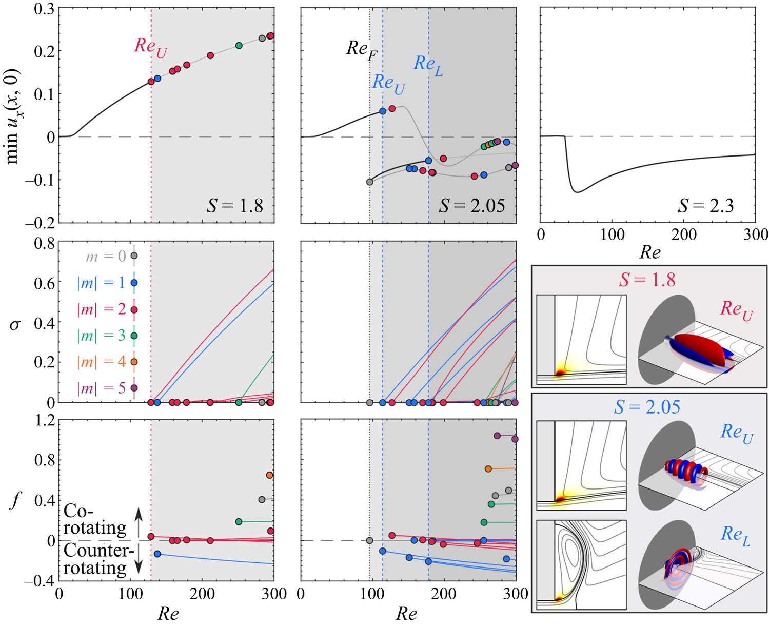
Figure 3. Bifurcation diagrams showing how the steady flow's minimum centreline velocity and the growth rate and frequency of the non-stable disturbances develop with  $\textit {Re}$ for
  $S=1.8$,
  $S=2.05$ and
  $S=2.3$. Bifurcation points are outlined in black and filled according their azimuthal periodicity as indicated. Visualisations of the critical disturbance modes at
  $\textit {Re}_U$ for
  $S=1.8$ and
  $S=2.05$ as well as
  $\textit {Re}_L$ for
  $S=2.05$ are also presented. The visualisations include meridional projections of the structural sensitivity map with overlaid steady flow streamlines and isometric views of the three-dimensional azimuthal vorticity field at isocontour levels corresponding to
  $\pm 20\,\%$ of the maximum.
All of the fixed- $S$ cases exhibit similar behaviour for
  $\textit {Re}\lesssim 10$. Beginning at the Stokes (
 $\textit {Re}\leftarrow 0$) limit, the system is elliptic and linear, and the viscous swirling flow emerges from the pipe and quickly dissipates without ever forming a separating shear layer or recirculation zone. As
  $\textit {Re}$ increases to
  $\sim 10$, a shear layer forms that separates from the pipe's lip at
  $x=0$. In addition, nonlinearity gives rise to centrifugal effects proportional to
  $S^{2}$ which cause the jet to expand radially outward. Note that, as mentioned in § 2, the shape and thickness of the boundary layers in the pipe are essentially independent of the Reynolds number since the incoming flow is fully developed. Instead, the primary effect of increasing
  $\textit {Re}$ is to reduce the role of viscosity after the flow exits the rotating pipe.
With the exception of very low Reynolds numbers, where it dissipates too quickly to form a distinct jet, the steady flow at  $S=1.8$ takes the form of a quasi-columnar swirling jet without any noticeable deceleration along the central axis (see pattern 2 from figure 2). In this case, the value of
  $\min u_x(x,0)$ reported in figure 3 is equivalent to the centreline velocity at the domain exit
  $u_x(R_\infty ,0)$ which slowly rises with increasing
  $\textit {Re}$ as the dissipation decreases. The axisymmetric equilibrium manifold at
  $S=1.8$ is single valued for all relevant
  $\textit {Re}$. However, this steady flow solution only remains stable up to
  $\textit {Re}_U=128.8$. At this point, the steady flow experiences a Hopf bifurcation associated with a co-rotating
  $|m|=2$ mode. As
  $\textit {Re}$ increases further, the flow becomes even more unstable, both due to the rising growth rate of the existing unstable mode and due to new instabilities which occur in subsequent bifurcations.
At  $S=2.05$, the jet has up to three steady solutions for the range of
  $\textit {Re}$ investigated. These include one solution curve connected to the Stokes solution in the
  $\textit {Re}\rightarrow 0$ limit, and a pair of solutions disconnected from the first which stem from a saddle-node bifurcation at
  $\textit {Re}_F=95.82$. Setting aside the issue of instability for a moment, the upper solution branch represents a quasi-columnar jet flow for
  $\textit {Re}\lesssim 140$. As
  $\textit {Re}$ increases beyond this value, the streamlines along the axis bulge outwards until a central bubble-type recirculation zone gradually emerges at
  $\textit {Re}\sim 168$ without bifurcation. For
  $\textit {Re}>168$, the recirculation zone enlarges and eventually gives way to various multi-cellular recirculation features similar to those found in the axisymmetric simulations of Ruith et al. (Reference Ruith, Chen, Meiburg and Maxworthy2003). However, since these steady solutions are linearly unstable to a broad range of three-dimensional disturbances, we will not investigate them in detail here. In contrast to the upper solution branch, both solutions of the pair which appear at
  $\textit {Re}_F$ always exhibit at least one central stagnation point. At
  $\textit {Re}=100$, these fixed-
 $S$ solutions correspond to the second and third solution segments from the fixed-
 $\textit {Re}$ results described in the previous subsection. As was the case there, the saddle solution (lower grey curve in figure 3) exhibits a transitional structure between bubble-type and cone-type central recirculation features (see pattern 5 and 6 from figure 2), while the node solution (lower black curve in figure 3) represents a flared-open cone structure dominated by a strong outer ring vortex (see patterns 6 and 7 from figure 2). Qualitatively, these structures persist as
  $\textit {Re}$ varies, although the recirculation zones become significantly larger as
  $\textit {Re}$ increases.
Returning to the question of stability, the steady flow at  $S=2.05$ is stable and single valued until the saddle-node bifurcation at
  $\textit {Re}_F$. The newly born saddle solution branch is unstable with respect to non-oscillatory
  $m=0$ perturbations throughout its existence, but both of the other branches remain linearly stable until Hopf bifurcations occur at
  $\textit {Re}_U=113.8$ on the quasi-columnar solution branch and at
  $\textit {Re}_L=177.6$ on the lower branch. Unlike the
  $S=1.8$ case which had a leading instability associated with
  $|m|=2$, the bifurcations in this case are both associated with counter-rotating
  $|m|=1$ modes. Shortly after their leading
  $|m|=1$ instability, both of the now-unstable branches experience additional bifurcations associated with co-rotating
  $|m|=2$ modes followed by a variety of others.
Finally, we consider the case of  $S=2.3$. At this high level of rotation, the steady solution curve is again single valued over the relevant range of Reynolds numbers. As
  $\textit {Re}$ increases away from the Stokes limit, the flow quickly transitions into a radial wall-jet solution with an enormous central recirculation zone (similar to pattern 8 from figure 2). The fluid's inertia increasingly resists this abrupt lateral reorientation of the flow, resulting in the formation of a ring-shaped separation vortex surrounding the pipe exit (similar to pattern 7 from figure 2) which grows with
  $\textit {Re}$. The strongly swirling flow remains stable well beyond the critical Reynolds numbers of previous cases, eventually succumbing to a co-rotating
  $|m|=1$ Hopf bifurcation at
  $\textit {Re}=348.4$.
4.3. Discussion: overall steady flow characteristics
Having separately considered the steady flow's behaviour at constant  $\textit {Re}$ and
  $S$, we conclude our analysis of the steady flow with a more holistic perspective toward its overall dynamics. The single-parameter bifurcation curves discussed previously represent one-dimensional slices cut from a two-dimensional manifold of steady solutions over the
  $(\textit {Re},S)$ parameter space. Likewise, the bifurcation points from the earlier diagrams are extended into neutral curves delimiting the steady flow's dynamically distinct regions. Taken together, this analysis synthesises calculations from over 20 000 distinct steady states. The resulting three-dimensional bifurcation diagram is presented in figure 4 along with a stability map formed by projecting the neutral curves from the solution manifold onto the
  $\textit {Re}$–
 $S$ plane. The stability map provides a comprehensive overview of the dynamics of the free swirling jet steady flow over the region
  $(\textit {Re},S)\in [0,0]\times [300,3]$ while the bifurcation diagram provides a more detailed representation of the state-space topology for
  $(\textit {Re},S)\in [40,1.8]\times [200,2.3]$.

Figure 4. (a) Three-dimensional bifurcation diagram and (b) two-dimensional stability map for the swirling jet steady flow. Each neutral curve delimits the locus of critical points corresponding to each value of  $m$. Thus, criticality occurs at the outermost neutral curve along the manifold. Points where the neutral curves of the leading and secondary eigenmodes cross are indicated by small filled circles.
Figure 4 indicates that bistability between two distinct axisymmetric steady states exists over a range of swirl and Reynolds numbers. This transition to bistable behaviour is triggered by a codimension-2 cusp bifurcation at  $(\textit {Re},S)=(47.10,2.175)$, well before any of the oscillatory linear modes are destabilised. These results shed light on the different physics and sequences of bifurcations between laterally confined and unconfined flows. In confined flow situations, bistability typically occurs between steady columnar and breakdown states, as demonstrated theoretically (Lopez Reference Lopez1994; Wang & Rusak Reference Wang and Rusak1997; Meliga & Gallaire Reference Meliga and Gallaire2011) and evidenced experimentally (Sarpkaya Reference Sarpkaya1971). Thus, vortex breakdown in confined flows is typically associated with an abrupt, hysteretic transition as the swirl parameter increases. In this unconfined flow, however, bistability is not associated with the initial occurrence of vortex breakdown. Rather, it results from a competition and interaction between the secondary recirculating flow surrounding the jet and the central recirculation zone as described in § 4.1. As the central recirculation zone grows in size, its relative strength compared with the outer recirculation zone decreases, resulting in a sudden transition from a breakdown state with a small central bubble to a cone or wall-jet state with a ring-shaped separation vortex around the pipe exit as
  $S$ increases beyond
  $S_B$. This distinction raises an important practical consideration: What radius is required of a closed experimental apparatus to approximate an unconfined flow? While we have not directly studied the effect of lateral confinement, our results along the intermediate and lower solution manifolds show significant radial flow across the open boundary which would clearly be affected by the introduction of a solid lateral wall. This suggests that any experimental device attempting to avoid confinement effects should at least exceed the radial extent of the unconfined domain used in this study.
Our results should also be contrasted with results from unconfined swirling flows with widespread axial co-flow. Meliga et al. (Reference Meliga, Gallaire and Chomaz2012) have shown that the steady solution manifold for the Grabowski–Berger vortex is single valued for  $\textit {Re}\leq 300$ and that a central recirculation zone appears gradually in the flow field as the swirl parameter increases. This qualitatively different result from those reported here appears to stem from the axial co-flow surrounding the vortex centre in that model, which suppresses the formation of an outer recirculation zone. This, in turn, prevents the competing physics which lead to bistability and hysteresis of the steady flow. This suggests that if the velocity of the co-flow surrounding the jet is decreased, a threshold will be reached where an outer recirculation region can form and potentially give rise to bistable behaviour. While we are not aware of any studies which have directly investigated this idea, Moise & Mathew (Reference Moise and Mathew2019) have explored the dynamics of the more jet-like ‘Maxworthy’ swirling flow model with a widespread, but very weak axial co-flow fixed to 1 % of the core velocity. They presented evidence of hysteresis between bistable breakdown states similar to those detailed in this study, supporting the idea that the presence of an outer recirculation zone, enabled by a sufficiently weak axial co-flow, is necessary for bistability of the unconfined steady flow.
The diagrams in figure 4 also reveal that, for  $S\leq 3$ and
  $\textit {Re}\leq 300$, the initial transition to unsteady behaviour always originates at Hopf bifurcations associated with either
  $|m|=1$ or
  $|m|=2$ depending on the local flow state and parameter values. Nonetheless, particularly at higher
  $\textit {Re}$, additional instabilities of other azimuthal periodicities bifurcate from the unstable steady flow at parameter values beyond the primary
  $|m|=1$ or
  $|m|=2$ instabilities. For example, the Hopf bifurcations associated with
  $m=0$ occur at parameter values well beyond the critical values of the leading non-axisymmetric modes. Even though
  $|m|=1$ has a lower minimum critical
  $\textit {Re}$, it is clear from the diagrams that
  $|m|=2$ is typically destabilised at lower values of swirl on the upper manifold. Regardless, the steady solution manifold is unstable toward both modes over an appreciable portion of the parameter space which is not limited to the quasi-columnar flow regime. This will be explored further in the following section which focuses on the periodic solution branches.
5. Characterisation of limit cycle states
In this section, we turn our attention to the structure and dynamics of the time-periodic solutions originating from Hopf bifurcations of the steady flow. These nonlinear solution branches are traced using the continuation method described in § 3.2.4 which plainly reveals saddle-node bifurcations of limit cycles and allows identification of multi-stable periodic states. However, temporal behaviours beyond those characterised here are certainly likely, as we have not sought periodic orbits which are disconnected from the steady flow solution manifold, determined the Floquet stability of the identified periodic states, or considered quasiperiodic or chaotic dynamics.
Compared with the steady flows examined previously, the flow topology and nonlinear dynamics of the periodic solution branches tend to be significantly more complex. Nonetheless, as in § 4,  $\min u_x(x,0)$ is again useful for monitoring the evolution of the overall flow structure as the parameters are varied due to its relation to the vortex breakdown phenomenon. Importantly, even though the flow fields are unsteady, this minimum represents a static value corresponding to the axisymmetric mean flow component in order to satisfy continuity for non-axisymmetric oscillations. In addition to the minimum axial velocity along the centreline, we also monitor periodic solutions through the frequency and amplitude of the oscillation. Henceforth, the reported frequency and azimuthal periodicity values for a given limit cycle correspond to its fundamental oscillation. It should be noted, however, that the limit cycles do contain higher temporal and azimuthal harmonics due to nonlinearity which are accounted for in our results. The limit cycle amplitude is defined by the unsteady energy norm
  $\|\boldsymbol {\acute {u}}\|=\|\boldsymbol {u}-\boldsymbol {\bar {u}}\|$ which includes contributions from the fundamental oscillation and all resolved harmonics over the full domain.
5.1. The quasi-columnar jet regime
We begin our study of the periodic orbits by characterising their dynamics in the quasi-columnar flow regime. As apparent from the previous section, and particularly figure 4, for  $S\lesssim 2$, the flow assumes a quasi-columnar jet structure, and the steady solution manifold is single valued. In this low-swirl regime, the steady flow experiences its primary linear instability via Hopf bifurcations associated with
  $|m|=1$ and
  $|m|=2$ modes above certain critical parameter values. According to figure 3, as the Reynolds number increases beyond
  $\sim$160, a number of additional
  $|m|=2$ (and, eventually,
  $|m|=3$ and other) modes bifurcate from the quasi-columnar steady flow, which each give rise to their own distinct periodic solution branches. To start, we will consider relatively low Reynolds number to focus our analysis on the leading
  $|m|=1$ and
  $|m|=2$ periodic orbits in the quasi-columnar regime. The bifurcation diagrams for this case are presented in figure 5. The dynamics of the quasi-columnar flow at higher-
 $\textit {Re}$ will be considered near the end of this section.

Figure 5. Bifurcation diagrams showing the evolution of the minimum centreline velocity, amplitude and frequency of the periodic solutions (left) with varying  $S$ for
  $\textit {Re}=125$ and
  $\textit {Re}=150$ and (right) with varying
  $\textit {Re}$ for
  $S=2$. The steady solution curves are shown for reference in black, while the blue and red curves correspond to the
  $|m|=1$ and
  $|m|=2$ periodic solution curves, respectively. Outlined circles represent Hopf bifurcation points. The dotted light vertical lines indicate the intersections of the parameter sweeps at
  $(\textit {Re},S)=(125,2)$ and
  $(150,2)$. The periodic solutions at
  $(\textit {Re},S)=(150,2)$ are visualised in figure 6.

Figure 6. Visualisations of  $|m|=1$ (top two rows) and
  $|m|=2$ (bottom two rows) limit cycle oscillations at
  $(\textit {Re},S)=(150,2)$ via streamlines and axial velocity contours over
  $(x,r,\theta )\in [-1,5]\times [0,3]\times [0,2{\rm \pi} ]$. The top and bottom image sequences show (from left to right) axial slice planes at
  $x=1/2,1,2$ of the instantaneous flow as viewed from downstream along with a three-dimensional isometric view. The middle image sequences show meridional slice planes at three equally spaced phase points with time increasing from left to right, followed by a comparison of the associated mean (top half) and steady (bottom half) flow. The dashed circle on each axial slice plane indicates the position of the pipe wall. The dotted lines show the intersection of the axial and meridional planes at each point of phase, with arrows in the axial planes indicating how these lines move with time. The yellow and black surfaces in the isometric views represent the respective positive and negative isocontour values indicated in the figure.
Figure 5 demonstrates distinct bifurcation behaviours for the  $|m|=1$ and
  $|m|=2$ critical modes. For the
  $|m|=1$ oscillation, the limit cycle consistently departs from the steady solution manifold via supercritical Hopf bifurcations. Conversely, for
  $|m|=2$, the bifurcation is subcritical, as finite-amplitude limit cycle states exist prior to the
  $|m|=2$ Hopf points. In both cases, the oscillation frequency is insensitive to
  $S$ but decreases noticeably with increasing
  $\textit {Re}$. The multivaluedness displayed by the solution curves in the bifurcation diagram indicates the possibility of multistability with respect to the steady flow and the
  $|m|=1$ and
  $|m|=2$ cycles. In addition, the fact that the
  $|m|=1$ and
  $|m|=2$ cycles coexist for an appreciable range of swirl suggests that a quasiperiodic orbit containing elements of both cycles could exist nearby in the state space.
We now move on to describing the morphology of the periodic flow states in this flow regime. At the parameter values discussed in this section, the mean flow structure of all limit cycles remains quasi-columnar (i.e.  $\min u_x(x,0)=u_x(R_{\infty },0)$), and the unsteady flow patterns are not strongly affected by the parameters. Figure 6 presents mean and instantaneous flow visualisations of the
  $|m|=1$ and
  $|m|=2$ limit cycles at
  $(\textit {Re},S)=(150,2)$ along with a depiction of the corresponding steady flow. Animated visualisations of these periodic flow states have also been provided in supplementary movies 1 and 2, available at https://doi.org/10.1017/jfm.2021.615, respectively. Note that the phase references selected to define
  $\theta =0$ and
  $t=0$ for these visualisations are arbitrary due to the system's
  $\theta$ and
  $t$ invariance. This invariance property also allows the time evolution of non-axisymmetric structures to be understood equivalently by rotation. In forward time, translation along
  $\theta$ proceeds in the opposite direction as the motion of the unsteady structures due to our convention that the signed value of
  $m$ be non-positive.
Beyond their distinct azimuthal periodicities, the  $|m|=1$ and
  $|m|=2$ limit cycles correspond to completely different patterns of unsteady flow which lead to major differences in their overall structure and dynamics. The leading
  $|m|=1$ limit cycle is associated with Kelvin–Helmholtz-like roll-up of the shear layer surrounding the jet. On an instantaneous basis, this limit cycle manifests itself as a nearly helical, counter-rotating, co-winding flow structure concentrated near the pipe exit. Based on this topology, it seems likely that the
  $|m|=1$ oscillation is driven primarily by the shear mechanism discussed in § 1. The
  $|m|=1$ oscillation does not significantly alter the quasi-columnar jet's mean momentum distribution over the parameter range studied here as there is relatively small topological difference between the axisymmetric mean flow associated with the
  $|m|=1$ limit cycle and the corresponding steady flow at identical parameter values. This similarity between the steady and mean flow fields is further demonstrated by the small effect of the
  $|m|=1$ oscillation on
  $\min u_x(x,0)$ as apparent in the bifurcation diagrams of figure 5.
The leading  $|m|=2$ limit cycle represents an oscillation of the swirling jet which is strikingly similar to the pre-breakdown
  $|m|=2$ instability described in the experiments of Billant et al. (Reference Billant, Chomaz and Huerre1998). The unsteady flow features a large, slowly co-rotating spiral structure which yields distinctive trident- and S-shaped flow patterns when visualised via meridional and axial slice planes, respectively. Unlike the relatively small and almost helical vortex roll-up associated with the
  $|m|=1$ oscillations, the
  $|m|=2$ limit cycle features substantial velocity fluctuations which extend several diameters axially and radially from the pipe exit. This reach leads to much higher entrainment of the fluid surrounding the jet than is present in either the steady flow or the
  $|m|=1$ limit cycle states. Because the jet's momentum is vigorously redistributed radially outward by these oscillations, there are significant differences between the topology of the mean flow states and the corresponding steady flow states. Even though the mean flow associated with the
  $|m|=2$ oscillations is quasi-columnar at
  $\textit {Re}=150$ in the sense that there is no centreline stagnation zone, the additional mixing provided by the unsteady flow leads to a region of strongly non-parallel flow in the vicinity of the pipe exit. This abrupt deflection of the mean flow leads to a significant reduction in the minimum centreline velocity associated with the
  $|m|=2$ limit cycle as shown in figure 5. Nonetheless, as the Reynolds number increases and the oscillation amplitude rises, the growing momentum deficit near the centreline eventually gives rise to an off-axis precessing stagnation point, triggering vortex breakdown.
Before ending this section, we briefly address the periodic solutions present in the quasi-columnar regime at higher Reynolds numbers. Many of these periodic orbits feature multi-valued solution manifolds, and their structures are associated with a broad range of wavenumbers and frequencies. For this reason, we only provide some illustrative examples of the numerous limit cycles which come into existence as  $\textit {Re}$ increases. Figure 7 displays a bifurcation diagram showing the dynamics of the quasi-columnar flow oscillations at
  $\textit {Re}=300$ alongside corresponding visualisations at selected points. Animations are also given for the
  $m=0$ and
  $|m|=3$ oscillations in supplementary movies 3 and 4, respectively.

Figure 7. Visualisations of selected limit cycles at  $\textit {Re}=300$ at the points indicated by the small points in the corresponding bifurcation diagram. Flow visualisations follow the format of figure 6, although only a single meridional and axial slice plane is shown for each solution. Recall that the arrows on the axial slice planes indicate the motion of the dotted line showing the plane intersections, not the motion of the flow field. Three-dimensional representations are also provided in the case of the
  $m=0$ and
  $|m|=3$ limit cycles.
The counter-rotating  $|m|=1$ and co-rotating
  $|m|=2$ limit cycles shown in the bifurcation diagram of figure 7 exhibit similar dynamics and structures to their lower-
 $\textit {Re}$ analogues, albeit with higher oscillation amplitudes. One key distinction, however, is that an entire ‘family’ of structurally similar, slowly co-rotating
  $|m|=2$ cycles are apparent rather than a single
  $|m|=2$ oscillation, testifying to the strong non-normality arising in the system as
  $\textit {Re}$ increases. Moreover, the diagram also indicates the presence of new counter-rotating
  $|m|=2$ limit cycles. These oscillations are associated with a separate instability which will be discussed below alongside figure 10.
For now, we will turn our attention to solutions with other wavenumbers, beginning with  $m=0$. The axisymmetric oscillation bifurcates in a subcritical manner from the steady flow at
  $S=1.718$ but its solution curve almost immediately turns forward in a saddle-node bifurcation. This oscillation leads to the formation of axisymmetric vortex rings near the pipe exit which, as shown in supplementary movie 3, propagate downstream along the jet's shear layers. Like the
  $|m|=1$ shear layer oscillations studied above, the
  $m=0$ limit cycle has an almost negligible effect on the mean flow. However, compared with the ‘bending’
  $|m|=1$ oscillations, these ‘bulging’
  $m=0$ structures are both more stable (in the sense that they require higher
  $\textit {Re}$ and
  $S$ values to bifurcate) and weaker (as their overall amplitude is smaller). The clear difference between these results and those in experiments which often include axisymmetric vortex shedding at pre-breakdown conditions (Billant et al. Reference Billant, Chomaz and Huerre1998; Loiseleux & Chomaz Reference Loiseleux and Chomaz2003; Liang & Maxworthy Reference Liang and Maxworthy2005) is noteworthy. This distinction may be related to the jet exit profile, as those experiments tend to have thinner boundary layers while the jet profile used here is fully developed. As shown by Michalke (Reference Michalke1984), the inviscid linear dynamics of fully developed jets is dominated by
  $|m|=1$ disturbances, while jets with thinner boundary layers tend to prefer
  $m=0$ modes. In either case, Reference MichalkeMichalke's (Reference Michalke1984) review for non-swirling jets suggests only passive convective instability, a viewpoint also supported by the experiments mentioned in § 1. Nonetheless, as our results do show evidence of self-excited behaviour for both
  $m=0$ and
  $|m|=1$ modes at moderate swirl levels, it seems likely that sharper shear layers would preferentially promote the axisymmetric oscillation.
Figure 7 also highlights the role of higher-wavenumber oscillations in the dynamics at  $\textit {Re}=300$. While the amplitudes of these
  $|m|\geq 3$ instabilities are clearly dwarfed by the
  $|m|=2$ ‘Billant’ instability discussed earlier for all relevant
  $S$, their dynamics may still be relevant to physical situations. In particular, the emergence of the
  $|m|=3$ oscillation at relatively low
  $S$ and high
  $\textit {Re}$ in our results is qualitatively consistent with the experimental observations of Billant et al. (Reference Billant, Chomaz and Huerre1998) and Liang & Maxworthy (Reference Liang and Maxworthy2005), although their transitions occurred at significantly higher Reynolds numbers. This indicates that a periodic attractor with
  $|m|=3$ which bifurcates from the steady flow could be responsible for their observed transition. Furthermore, the demonstrated existence of other limit cycle states with even higher periodicities suggests that such structures may represent relevant attractors for certain other high-
 $\textit {Re}$ conditions.
5.2. The vortex breakdown regime
In this section, we turn our focus to the various periodic states present at intermediate swirl levels where the steady flow transitions from a quasi-columnar jet to a lateral jet along the dump plane wall. According to figure 4, the steady flow solution manifold in this regime is characterised by multivaluedness over  $2\lesssim S\lesssim 2.1$. The drastic changes in steady flow topology and recirculation characteristics associated with the vortex breakdown phenomenon correspond to similarly dramatic shifts in the behaviour of the periodic solutions. As before, the number of periodic solutions present at intermediate swirl rises dramatically as the Reynolds number increases. For practical reasons, we have therefore limited our analysis in this section to
  $\textit {Re}\leq 200$.
Beginning with the case of  $\textit {Re}=150$, the evolution of the periodic solutions with changing
  $S$ are shown in the bifurcation diagrams and visualisations of figure 8. The solutions detailed in this diagram begin near the end of the quasi-columnar flow regime at
  $S=2$. As the rotation is increased beyond this value, the vortex breakdown phenomenon begins to manifest itself on the periodic and steady solutions. However, compared to the steady solutions, the periodic solutions clearly require a higher value of
  $S$ in order to form a central recirculation zone. We suspect that this may be attributed to the increased mixing associated with the oscillations resisting the central momentum deficit required to yield an internal stagnation point. Nonetheless, once the central recirculation zone does form, the
  $|m|=1$ and
  $|m|=2$ oscillations are both rapidly quenched as the bubble enlarges. Both the
  $|m|=1$ and
  $|m|=2$ oscillations restabilise before the first saddle-node bifurcation of the steady flow is encountered at
  $S_B$, leading to a brief interval of stability of the steady flow corresponding to a steady ‘bubble’ breakdown state.

Figure 8. Bifurcation diagram for  $\textit {Re}=150$ at intermediate swirl showing the evolution of the minimum centreline velocity, amplitude and frequency with
  $S$ along with instantaneous and mean flow visualisations using the format of figure 6 at the indicated points. Only one phase point of the instantaneous flow is shown. Note that the three-dimensional isocontours from this figure onward correspond to radial velocity fluctuations, unlike the isocontours for axial velocity fluctuations shown in § 5.1.
As  $S$ decreases along the intermediate solution manifold after reaching
  $S_B$, the steady solution curve is initially only unstable with respect to a non-oscillatory
  $m=0$ mode as discussed in § 4.1. However,
  $|m|=1$ and 2 Hopf bifurcations eventually do give rise to non-axisymmetric periodic solutions which branch from the steady solution. These limit cycle oscillations feature cone-shaped central recirculation zones which are clearly different from the bubble-shaped recirculation zones associated with their analogues along the upper solution manifold. Nonetheless, the unsteady structures and frequencies associated with both oscillations remain qualitatively similar to the
  $|m|=1$ and
  $|m|=2$ structures from before.
We now proceed to a higher Reynolds number case at  $\textit {Re}=200$. Figure 9 includes all of the periodic solution branches detected on the presented interval. Clearly, many more distinct limit cycles are present at
  $\textit {Re}=200$ than at
  $\textit {Re}=150$, indicating a dramatic rise in complexity. Nonetheless, it should again be emphasised that even more complex behaviour is possible. The system may support or favour quasiperiodic and/or chaotic attractors over the purely periodic solutions considered here.

Figure 9. Bifurcation diagram for the steady and periodic solutions at  $\textit {Re}=200$ and intermediate swirl showing the evolution of the minimum centreline velocity, amplitude and frequency with
  $S$. The periodic solution branches are labelled sequentially in the order of appearance of their terminal bifurcation points along the steady flow solution curve.
The analysis in § 4 indicated that several different instabilities with  $|m|=1$ and
  $|m|=2$ exist at
  $\textit {Re}=200$. The periodic solutions present in the quasi-columnar flow regime before breakdown can be seen in figure 9 as the periodic solution curves with non-zero amplitude at
  $S=2$, i.e. curves 1–5. The solutions numbered 1 through 3 consist of a family of slowly co-rotating
  $|m|=2$ oscillations which include the
  $|m|=2$ instability described in § 5.1 on branch 1 and other similar, but more spatially extended oscillations on branches 2 and 3. These branches disappear as the penetration depth of the jet decreases with increasing
  $S$ due to the higher entrainment and, eventually, the emergence of the central stagnation region. Similarly, solution branch 4, an
  $|m|=1$ oscillation, represents the same
  ${|m|=1}$ instability of the quasi-columnar flow seen in figure 8. Neither the morphology nor the frequency of the
  $|m|=1$ oscillation changes significantly from the
  $\textit {Re}=150$ case, although its dynamics does show a pleated pair of saddle-node bifurcations at
  $\textit {Re}=200$ which was not present before. Finally, solution branch 5 corresponds to a counter-rotating
  $|m|=2$ oscillation which was also apparent in figure 7.
Visualisations of the flow structures on branch 5 are shown in figure 10 and animated in supplementary movie 5. In the quasi-columnar flow regime, its unsteady motion takes the form of a long, counter-rotating, co-winding double spiral. As the rotation increases, this structure gradually moves upstream until it eventually interacts with the recirculating flow along the wall near the pipe exit. Even when the flow along the centreline is everywhere positive, these strong near-wall velocity fluctuations produce powerful Reynolds stresses which greatly assist entrainment and dramatically distort the mean flow near the pipe exit in comparison with the steady flow. As  $S$ increases further, the growing interactions between the near-wall fluctuations and the mean flow reduce the penetration of the jet and cause the outer recirculation features to further dominate the flow dynamics. Eventually, this dynamics reaches a crux signalled by the appearance of a saddle-node bifurcation concurrent with stagnation of the on-axis flow. From this point onwards, the separation vortex overwhelmingly dominates the flow behaviour, rapidly pulling the initial stagnation point open into a massive region of reversed flow which deflects the jet radially outwards until it attains a wall-jet morphology and eventually terminates along the lower part of the steady solution manifold.

Figure 10. Visualisation of the flow structures at two points along branch 5 of figure 9. Both representations are extracted from the volume  $(x,r,\theta )\in [-2,10]\times [0,6]\times [0,2{\rm \pi} ]$.
After the emergence of the central recirculation zone, the periodic solution curves consist of co- and counter-rotating  $|m|=1$ and
  $|m|=2$ oscillations superposed upon non-columnar mean flow fields. For example, representative visualisations of solution branch 6, which corresponds to a co-rotating
  $|m|=1$ oscillation, are shown in figure 11 and supplementary movie 6. Initially, the morphology of the solutions on branch 6 take the form of a gently azimuthally precessing ellipsoidal ‘bubble’ recirculation region with a counter-winding spiral tail similar to the structure described in the simulations of Ruith et al. (Reference Ruith, Chen, Meiburg and Maxworthy2003). It is clear by comparison with the steady flow solutions along the intermediate manifold that these
  $|m|=1$ oscillations dramatically limit the size of the mean recirculation zone. However, as
  $S$ decreases in this unconfined flow, the small recirculation bubble rapidly opens up into a much larger asymmetric cone structure resembling the observations of Billant et al. (Reference Billant, Chomaz and Huerre1998).

Figure 11. Visualisation of the flow structures at  $S=2.05$ along branch 6 of figure 9. The visualised volume is
  $(x,r,\theta )\in [-2,10]\times [0,6]\times [0,2{\rm \pi} ]$.
As another example, solution branch 7, which corresponds to counter-rotating  ${|m|=2}$ oscillations, is visualised in figure 12 and supplementary movie 7. The unsteady structures on curve 7 take the form of vortex filaments arranged in a co-winding double spiral concentrated along the shear layers between the jet and the inner and outer recirculation zones. These shear layer fluctuations greatly enhance mixing of the jet fluid with its surroundings. At first, these oscillations primarily entrain fluid from the central recirculation zone, causing the time-averaged central recirculation zone to radially compress and axially elongate relative to the corresponding steady flow field. This ‘squeezing’ of the central bubble allows the solutions along curve 7 to exhibit more negative velocities along the axis than the steady flow and stalls the expansion of the central bubble with decreasing swirl. However, as rotation further decreases and the central recirculation bubble begins to swell, these oscillations begin to instead favour entrainment from the outer recirculation zone. This transition reverses the previous trend whereby the mean central vortex bubble is compressed, rather causing the central recirculation zone to expand to a larger size than is seen in the steady flow. Nonetheless, this expansion of the central vortex weakens the oscillation, leading to a complex chain of nonlinear behaviours which manifest a pleated pair of saddle-node bifurcations and ultimately result in the demise of the solution curve.

Figure 12. Visualisation of the flow structures at two points along branch 7 of figure 9. In both cases, the visualised volume is  $(x,r,\theta )\in [-2,10]\times [0,6]\times [0,2{\rm \pi} ]$.
For completeness, we also briefly describe the solutions along branches 8–10. Solution branch 8 is a co-rotating  $|m|=2$ instability as shown by the representative visualisations in figure 13 and supplementary movie 8. The solutions on branch 8 can be interpreted as the
  $|m|=2$ analogue of the
  $|m|=1$ solutions on branch 6. That is, they correspond to oscillatory motions featuring a pulsating, non-axisymmetric ellipsoidal recirculation bubble with a counter-winding spiral tail. This structure closely resembles the ‘double-helical’ breakdown mode described in the Grabowski–Berger vortex simulations of Ruith et al. (Reference Ruith, Chen, Meiburg and Maxworthy2003). Much like the solutions on branch 6, these oscillations retard the expansion of the time-average central recirculation zone as
  $S$ decreases in comparison with the corresponding steady flow solutions. Visualisations of representative solutions along curve 9 are also shown in figure 13 and in supplementary movie 9. Unlike branch 8, the
  $|m|=1$ oscillations on branch 9 do not have a significant influence on the overall size of the recirculation zone of the mean flow. Nonetheless, these oscillations do introduce a sizeable non-axisymmetric component to the central recirculation zone which causes a gentle, large-scale precession resulting in an asymmetric cone state similar to that described by Billant et al. (Reference Billant, Chomaz and Huerre1998). Finally, solution branch 10 represents a higher-
 $\textit {Re}$ occurrence of the same post-breakdown
  $|m|=1$ oscillation shown at
  $\textit {Re}=150$ in figure 8.

Figure 13. Visualisation of the flow structures of branches 8 (top row) and 9 (bottom row) of figure 9. The representations correspond to the visualisation volumes  $(x,r,\theta )\in [-2,10]\times [0,6]\times [0,2{\rm \pi} ]$ and
  $(x,r,\theta )\in [-4,20]\times [0,12]\times [0,2{\rm \pi} ]$, respectively.
5.3. The wall-jet regime
After the flow transitions from a quasi-columnar jet to the wall-jet regime, the steady flow solution manifold once again becomes single valued for  $S\gtrsim 2.2$. As shown in figure 4, a co-rotating
  $|m|=1$ instability appears in this high-swirl regime for sufficiently high
  $\textit {Re}$. Note that this instability belongs to a different neutral curve than the other
  $|m|=1$ modes described in this study. Although other instabilities will certainly appear in this flow regime at higher parameter values, we detected no additional bifurcations for
  $S\leq 3$ and
  $\textit {Re}\leq 300$.
A bifurcation diagram and visualisation of the mean and instantaneous flow for the  $|m|=1$ limit cycle in the wall-jet regime at
  $\textit {Re}=300$ is presented in figure 14. A video showing the periodic motion through a complete oscillation is also included in supplementary movie 10. This limit cycle bifurcates in a supercritical manner with respect to its neutral curve and consists of a co-rotating, counter-winding radial spiral structure along the shear layer separating the spreading jet from the centrally recirculating fluid. This is clearly different from the
  $|m|=1$ shear layer instabilities covered earlier (e.g. at
  $S=2.05$,
  $\textit {Re}_L$ in figure 3) which instead feature oscillations localised to the shear layer separating the jet from the outer recirculating fluid. Nonetheless, this oscillation does not significantly influence the mean distribution of momentum, as can be seen by comparing the steady and time-averaged flows. Unlike the instabilities analysed earlier, this limit cycle generates a small, but noticeable, motion in the pipe immediately upstream of the dump plane due to a slight precession of the leading stagnation point near the exit plane. This suggests that at parameter values beyond those investigated here, the onset of breakdown in the pipe may be linked to three-dimensional (rather than axisymmetric) motions due to downstream conditions related to the dynamics of the free jet after it exits the pipe. This bears certain similarities to the three-dimensional scenarios for vortex breakdown of columnar flows in finite-length rotating pipes discussed by Wang et al. (Reference Wang, Rusak, Gong and Liu2016). Their linear analysis focused on the dynamics of propagating Kelvin waves which are trapped by the asymmetric streamwise boundary conditions and showed that, in certain cases, the primary instability in swirling pipe flow is non-axisymmetric. The configuration studied here, on the other hand, is much more complex, involving additional physical mechanisms both within and beyond the pipe as well as nonlinear effects.

Figure 14. Bifurcation diagram and visualisations for the  $|m|=1$ limit cycle in the wall-jet regime at
  $\textit {Re}=300$.
5.4. Discussion: overall limit cycle characteristics
This subsection reviews the results of our analysis of the swirling jet's periodic solutions and discusses them in the context of existing literature. Just as in § 4.3, the various limit cycle solution curves can be interpreted as solution manifolds over the ( $\textit {Re},S$) parameter space. However, many of these solution manifolds are multivalued over a significant portion of the parameter space due to subcritical bifurcation behaviours or other nonlinear effects and almost all overlap with other limit cycle manifolds in the
  $(\textit {Re},S)$ space. These qualities make a clear, global visualisation of the limit cycle dynamics analogous to figure 4 difficult to realise. Nonetheless, the results show that a variety of different limit cycle structures ranging in periodicity from
  $0\leq |m|\leq 5$ and exhibiting both co- and counter-rotating temporal behaviours and diverse spatial structures exist over a large portion of the parameter space.
The fact that limit cycle states with different periodicities, rotation directions, and winding orientations exist at identical points in the parameter space is remarkable. Throughout the literature of swirling flows, there is a wide range of reported properties of the observed periodic structures. For example, Ruith et al. (Reference Ruith, Chen, Meiburg and Maxworthy2003) noted in their survey that confined experiments have typically reported co-winding spiral structures while unconfined experiments have favoured the counter-winding orientation. Liang & Maxworthy (Reference Liang and Maxworthy2005) have similarly emphasised differences in the structures’ observed rotation direction and speed across different studies. In our study, we have not found any evidence to support the idea that the limit cycle states have a global preference toward a single rotation or winding direction. However, we have not carried out the Floquet analyses necessary to ascertain the limit cycles’ stability characteristics, which could be biased toward particular rotation or winding traits. This indicates an important direction for future work.
Another important takeaway from this section is the significance of high-order bifurcation behaviours. Limit cycle oscillations stemming from supercritical Hopf bifurcations with a third-order normal form have been documented in swirling jets by several authors (Liang & Maxworthy Reference Liang and Maxworthy2005; Oberleithner et al. Reference Oberleithner, Sieber, Nayeri, Paschereit, Petz, Hege, Noack and Wygnanski2011; Meliga et al. Reference Meliga, Gallaire and Chomaz2012; Manoharan et al. Reference Manoharan, Frederick, Clees, O'Connor and Hemchandra2020). However, we are not aware of swirling jet studies which have conclusively demonstrated the type of fifth- or higher-order Hopf bifurcations recorded here, although hysteresis behaviour consistent with this idea has been reported (Billant et al. Reference Billant, Chomaz and Huerre1998; Moise Reference Moise2020). Aside from its physical implications, this is an important distinction because standard weakly nonlinear methods which employ a third-order Stuart–Landau amplitude (Sipp & Lebedev Reference Sipp and Lebedev2007; Meliga et al. Reference Meliga, Gallaire and Chomaz2012; Manoharan et al. Reference Manoharan, Frederick, Clees, O'Connor and Hemchandra2020) cannot capture these types of bifurcation behaviours. Several of the bifurcations recorded in our study would require a higher-order weakly nonlinear expansion (e.g. Barkley, Tuckerman & Golubitsky Reference Barkley, Tuckerman and Golubitsky2000) to be modelled appropriately. Moreover, our results did not show any specific link between the nature of a bifurcation and the azimuthal periodicity, rotation direction, or winding orientation of its ensuing limit cycle structures. Indeed, the super- or sub-critical nature of a bifurcation is determined by nonlinear effects stemming from interactions among the limit cycle fundamental, its harmonics and the mean flow. Such behaviours cannot be understood based purely on linear dynamics, although, as pointed out by a referee, the presence of subcritical dynamics in swirling jets does underscore the significance of the linear transient growth phenomena due to non-normality.
Lastly, we consider the role of unsteady nonlinear interactions in the jet's limit cycle dynamics. Harmonic interactions represent a key aspect of any nonlinear oscillation. However, as evidenced by Sipp & Lebedev (Reference Sipp and Lebedev2007), in certain cases, their dominant effect amounts to a steady Reynolds stress which only impacts the mean flow, while, in others, they also lead to significant Reynolds stress oscillations which directly influence the flow's oscillatory behaviour. While modelling the latter situation requires nonlinear methods, in the former case, a linear analysis about the mean flow (based upon either a nonlinear calculation or an experimental measurement) can often assess some aspects of the oscillation such as its linear stability, relative shape and frequency with fair accuracy (Barkley Reference Barkley2006). This raises an important practical question: Is mean flow stability analysis a robust technique for characterising certain features of limit cycle oscillations in swirling jets? A recent analysis by Manoharan et al. (Reference Manoharan, Frederick, Clees, O'Connor and Hemchandra2020) has demonstrated that, in the specific situation of a turbulent swirling jet where the limit cycle oscillation appears at a supercritical Hopf bifurcation, the mean flow analysis approach is effective. However, it remains to be seen whether the same is true in general.
This question was addressed by performing linear stability calculations on mean flow fields associated with the limit cycle states presented above at several representative conditions, and comparing them with linear calculations from the steady flow and the fully nonlinear results. The results of this analysis are given in table 2, along with the percentage of the unsteady kinetic energy contained in the limit cycle fundamental. Many of these cycles clearly do not satisfy the marginal stability property (Sipp & Lebedev Reference Sipp and Lebedev2007), (i.e.  $\sigma _M=0$) implying that unsteady harmonic interactions do influence the limit cycle dynamics. Nonetheless, the results also indicate that, in most cases, surprisingly accurate estimates of the limit cycle oscillation frequency can be obtained using mean flow stability analysis, even when the growth rate is not small. Similar determinations have been reached for swirling jets in the turbulent regime by Oberleithner et al. (Reference Oberleithner, Sieber, Nayeri, Paschereit, Petz, Hege, Noack and Wygnanski2011), Tammisola & Juniper (Reference Tammisola and Juniper2016) and Mukherjee et al. (Reference Mukherjee, Muthichur, More, Gupta and Hemchandra2021), in addition to the more formal demonstration mentioned above by Manoharan et al. (Reference Manoharan, Frederick, Clees, O'Connor and Hemchandra2020). This outcome is particularly convenient for the interpretation of experimental data, where time averages are readily accessible. Of course, for computations, the mean flow itself must be determined prior to applying this analysis.
Table 2. Comparison of selected nonlinear limit cycle results with frequency predictions from linear stability calculations about the mean flow and steady flow. Here, % $KE_f$ is the percentage of the unsteady kinetic energy contained in the limit cycle fundamental,
  $f$ is the nonlinear limit cycle frequency,
  $\sigma _{M}$ and
  $f_{M}$ are the growth rate and frequency of the mean flow eigenvalue and
  $\sigma _{S}$ and
  $f_{S}$ are the growth rate and frequency of the steady flow eigenvalue. Movies are available at https://doi.org/10.1017/jfm.2021.615.
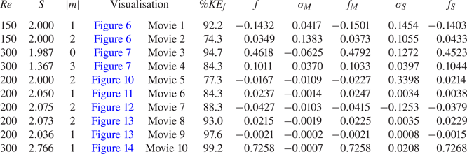
6. Conclusion
This investigation characterises the dynamics of an unconfined, fully developed swirling jet using bifurcation analysis. It shows how variations in the swirl ratio  $S$ and Reynolds number
  $\textit {Re}$ affect the morphology of the system's steady and time-periodic solutions and how the state-space topology of the associated solution manifolds are linked to the physical structure of the flow. The swirling jet transitions from a quasi-columnar jet along the central axis at low
  $S$ to a radial jet along the dump plane wall at high
  $S$. In between these limits, a nonlinear exchange of stability occurs due to a competition between two low pressure regions: a central region which is associated with vortex breakdown, and an outer region which forms due to entrainment of the ambient fluid exterior to the jet. This transition in flow structure is linked to a cusp bifurcation within the steady solution manifold which manifests parameter hysteresis over a small range of
  $S\sim 2$ for
  $\textit {Re}>47.1$.
Beyond certain critical parameter values, the steady solution manifold becomes unstable toward infinitesimal perturbations which break the time and azimuthal symmetry of the steady system. Over the range of parameters investigated, the initial Hopf bifurcations are always associated with  $|m|=1$ or
  $|m|=2$ disturbance modes. Additional instabilities corresponding to unsteady
  $m=0$ and
  $|m|\geq 3$ perturbations only occur at points on the solution manifold where at least one
  $|m|=1$ or
  $|m|=2$ mode is already unstable. The neutral curves associated with each linear disturbance mode represent the intersections of the various periodic solution manifolds and the steady solution manifold in the state space. The nonlinear limit cycle solutions which stem from these neutral curves are associated with both super- and sub-critical bifurcation behaviour. In the physical space, the limit cycle solutions display a wide array of three-dimensional, co- and counter-rotating flow structures which often exhibit very different time-averaged flow patterns compared against their steady counterparts at identical parameter values. Many of these structures bear strong resemblances to coherent structures reported in previous experiments. For example, the
  $|m|=2$ limit cycle in the pre-breakdown regime at
  $Re=150$ (see figure 6) is reminiscent of the
  $|m|=2$ instability detailed by Billant et al. (Reference Billant, Chomaz and Huerre1998). Similar parallels may also be drawn between the
  $|m|=1$ (figure 11) and
  $|m|=2$ (figure 13) periodic solutions which occur in the vortex breakdown regime at
  $Re=200$ and the single and double spiral forms of vortex breakdown reported in a broad range of swirling flows including top-hat jets (Liang & Maxworthy Reference Liang and Maxworthy2005), the Grabowski–Berger vortex (Ruith et al. Reference Ruith, Chen, Meiburg and Maxworthy2003) and confined vortex tubes (Sarpkaya Reference Sarpkaya1971), among others.
As remarked in § 1 and the previous paragraph, a unified framework that allows a global understanding of a general swirling flow configuration, and the similarities or distinctions between flow patterns across different flow configurations and parameter spaces, remains a key open challenge for the community. The present work contributes to this broader aim by definitively relating a suite of steady and time-periodic states in fully developed laminar swirling jets with flush injection into a semi-infinite reservoir. Nonetheless, further work will be necessary to extend these conclusions to a broader suite of swirling jet arrangements including, in particular, jets with thinner boundary layers and with varying levels of lateral and axial confinement. Additionally, limit cycle stability calculations (i.e. Floquet analysis) should be performed to identify transition to quasiperiodic and other higher dimensional dynamical behaviours.
Supplementary movies
Supplementary movies are available at https://doi.org/10.1017/jfm.2021.615.
Acknowledgements
C.D. acknowledges helpful discussions with Dr P. Jolivet from the Toulouse Institute of Computer Science Research and Dr V. Acharya from the Georgia Institute of Technology regarding the algorithms and parallel FreeFEM implementation used in this work.
Funding
This research has been partially funded by the U.S. Air Force Office of Scientific Research (contract number FA9550-16-1-0442, contract monitor Dr C. Li) and the University Turbine Systems Research Program (contract number DE-FE0031285, contract monitor Dr M. Freeman). The authors would also like to acknowledge high-performance computing support from Cheyenne (https://doi.org/10.5065/D6RX99HX) provided by NCAR's Computational and Information Systems Laboratory under project code UGIT0028 and sponsored by the National Science Foundation.
Declaration of interest
The authors report no conflict of interest.
Appendix A. Mesh sensitivity analysis
This appendix serves to assess the sensitivity of the presented results to the properties of the computational mesh. To achieve this, comparative calculations were performed against the primary mesh  $M$ using four test meshes
  $A_0$–
 $A_3$ listed in table 3. The properties of these test meshes were selected to separately assess specific details of the discretisation. In particular, the meshes
  $A_0$ and
  $A_1$ are used to assess the sensitivity of the results to the position of the respective inlet and open boundaries, while
  $A_2$ and
  $A_3$ gauge the sensitivity of the results to refining and coarsening the mesh, respectively.
Table 3. Comparison of mesh properties and critical  $S$ and
  $f$ values along the
  $Re=200$ steady solution curve. Here,
  $r_h$ is the mesh refinement factor relative to
  $M$ based on edge vertex density,
  $n_t$ is the total number of triangles and DOF is the total number of discrete degrees of freedom. As indicated in § 4, the saddle-node bifurcations at
  $S_B$ and
  $S_F$ are associated with non-oscillatory
  $m=0$ modes, while the Hopf bifurcations at
  $S_U$ and
  $S_L$ are associated with oscillatory
  $|m|=2$ and
  $|m|=1$ modes, respectively.

Bifurcation diagrams for  $Re=200$ with varying
  $S$ were computed on each mesh to quantify the dependence of the results on the mesh properties. The curves are almost indistinguishable from each other due to their similarity. To illustrate, the critical
  $S$ and
  $f$ values associated with the bifurcation points are tabulated in table 3. These data indicate excellent agreement across the various meshes as most numerical values are identical down to at least three significant digits. Consequently, we consider the results obtained on mesh
  $M$ to be well converged.
Appendix B. Numerical methods for periodic orbits
This appendix further details the algorithms and numerical tools used to solve (3.18) and allow the identification and continuation of periodic solutions as discussed in § 3.2.4. We first direct our attention to the algorithms, beginning with the fixed-parameter solver which iteratively refines an initial guess for a periodic orbit. This is analogous to the procedure for steady states associated with (3.5). For convenience, we introduce the following notation for the  $N$th-order discrete Fourier representation of a harmonic-balanced quantity with an azimuthally
  $m$-periodic fundamental component in real arithmetic,
 \begin{equation} \boldsymbol{\tilde{q}}_m^{N}= (\boldsymbol{\bar{q}}_0,\textrm{Re} \{\boldsymbol{\hat{q}}_m \},\textrm{Im} \{\boldsymbol{\hat{q}}_m \},\ldots,\textrm{Re} \{\boldsymbol{\hat{q}}_{Nm} \},\textrm{Im} \{\boldsymbol{\hat{q}}_{Nm} \})^{\mathrm{T}}. \end{equation}
 The solution process is based on a block factorisation scheme which algebraically isolates (3.18c) from the augmented system. In each step, we first find  $\boldsymbol {\tilde {v}}_m^{N}$ and
  $\boldsymbol {\tilde {a}}_m^{N}$ which satisfy
 \begin{gather} \mathcal{\tilde{J}}_m^{N} (\boldsymbol{\tilde{q}}_m^{N},f )\boldsymbol{\tilde{v}}_m^{N}= \mathcal{\tilde{R}}_m^{N} (\boldsymbol{\tilde{q}}_m^{N},f ), \end{gather}
 \begin{gather}\mathcal{\tilde{J}}_{m}^{N} (\boldsymbol{\tilde{q}}_m^{N},f )\boldsymbol{\tilde{a}}_m^{N}= \frac{\partial\mathcal{\tilde{R}}_m^{N} (\boldsymbol{\tilde{q}}_m^{N},f )}{\partial f}, \end{gather}
where  $\mathcal {\tilde {R}}_m^{N}(\boldsymbol {\tilde {q}}_m^{N},f)$ is the combined residual of (3.18a) and (3.18b) in real arithmetic,
  $\mathcal {\tilde {J}}_m^{N}(\boldsymbol {\tilde {q}}_m^{N},f)= \partial \mathcal {\tilde {R}}_m^{N}/\partial \boldsymbol {\tilde {q}}_m^{N}$ is the associated real Jacobian matrix given by
 \begin{equation} \begin{bmatrix} {\boldsymbol{\mathsf{J}}}_0 (\boldsymbol{\bar{q}}_0 ) & \textrm{Re} \{{\boldsymbol{\mathsf{H}}}_{0} (\boldsymbol{\hat{q}}_{m}^{*} )+{\boldsymbol{\mathsf{H}}}_{0}^{*} (\boldsymbol{\hat{q}}_{m} ) \}& \textrm{Im} \{-{\boldsymbol{\mathsf{H}}}_{0} (\boldsymbol{\hat{q}}_{m}^{*} )+{\boldsymbol{\mathsf{H}}}_{0}^{*} (\boldsymbol{\hat{q}}_{m} ) \}& \ldots \\ \textrm{Re} \{{\boldsymbol{\mathsf{H}}}_{m} (\boldsymbol{\hat{q}}_{m} ) \}& \textrm{Re} \{{\boldsymbol{\mathsf{L}}}_{m} (\boldsymbol{\bar{q}}_0,f )+{\boldsymbol{\mathsf{H}}}_{m}^{*} (\boldsymbol{\hat{q}}_{2m} ) \}& \textrm{Im} \{-{\boldsymbol{\mathsf{L}}}_{m} (\boldsymbol{\bar{q}}_0,f )+{\boldsymbol{\mathsf{H}}}_{m}^{*} (\boldsymbol{\hat{q}}_{2m} ) \}& \ldots \\ \textrm{Im} \{{\boldsymbol{\mathsf{H}}}_{m} (\boldsymbol{\hat{q}}_{m} ) \}& \textrm{Im} \{{\boldsymbol{\mathsf{L}}}_{m} (\boldsymbol{\bar{q}}_0,f )+{\boldsymbol{\mathsf{H}}}_{m}^{*} (\boldsymbol{\hat{q}}_{2m} ) \}& \textrm{Re} \{{\boldsymbol{\mathsf{L}}}_{m} (\boldsymbol{\bar{q}}_0,f )-{\boldsymbol{\mathsf{H}}}_{m}^{*} (\boldsymbol{\hat{q}}_{2m} ) \}& \ddots \\ \vdots & \vdots & \ddots & \ddots \end{bmatrix}, \end{equation}
and  $\partial \mathcal {\tilde {R}}_m^{N}/\partial f=2{\rm \pi} (0,-{\boldsymbol{\mathsf{M}}}\textrm {Im}\{\boldsymbol {\hat {q}}_{m}\}, {\boldsymbol{\mathsf{M}}}\textrm {Re}\{\boldsymbol {\hat {q}}_{m}\},\ldots ,-N{\boldsymbol{\mathsf{M}}} \textrm {Im}\{\boldsymbol {\hat {q}}_{Nm}\},N{\boldsymbol{\mathsf{M}}}\textrm {Re} \{\boldsymbol {\hat {q}}_{Nm}\})^{\mathrm {T}}$. The resolution of (B2) relies on iterative Krylov subspace methods as discussed below, and a significant savings is realised by applying the same factorisation of the preconditioner during the iterations for both equations.
Once intermediate vectors are obtained from (B2), the corrections which complete the Newton step for (3.18) are determined via
 \begin{gather} \delta f= \frac{(\boldsymbol{\tilde{\phi}}_m^{N})^{\mathrm{T}} \boldsymbol{\tilde{v}}_m^{N}}{(\boldsymbol{\tilde{\phi}}_m^{N})^{\mathrm{T}} \boldsymbol{\tilde{a}}_m^{N}}, \end{gather}
 \begin{gather}\delta\boldsymbol{\tilde{q}}_m^{N}= \boldsymbol{\tilde{v}}_m^{N}- \boldsymbol{\tilde{a}}_m^{N}\delta f, \end{gather}
where  $\boldsymbol {\tilde {\phi }}_m^{N}=(0,{\boldsymbol{\mathsf{M}}} \Re \{\boldsymbol {\hat {q}}_{m}\},-{\boldsymbol{\mathsf{M}}}\Im \{\boldsymbol {\hat {q}}_{m}\}, \ldots ,N{\boldsymbol{\mathsf{M}}}\Re \{\boldsymbol {\hat {q}}_{Nm}\},-N{\boldsymbol{\mathsf{M}}} \Im \{\boldsymbol {\hat {q}}_{Nm}\})^{\mathrm {T}}$ is a phase reference derived by linearising (3.18c). Then, the solution is updated as
  $(\boldsymbol {\tilde {q}}_m^{N},f)\leftarrow (\boldsymbol {\tilde {q}}_m^{N},f)- (\delta \boldsymbol {\tilde {q}}_m^{N},\delta f)$, and the process is repeated until the norm of the residual of (3.18) converges within the tolerance.
After a branch of periodic solutions has been identified, parametric continuation is performed using a Moore–Penrose predictor–corrector scheme in a similar manner to the approach based on (3.9). In the case where the periodic state is initialised from a Hopf point, the initial null vector is simply the bifurcating eigenvector. However, in general, the harmonic-balanced null vector  $\boldsymbol {\tilde {y}}=(\boldsymbol {\tilde {y}}_{\boldsymbol {q},m}^{N}, \tilde {y}_f,\tilde {y}_\alpha )^{\mathrm {T}}\in \ker (\mathcal {\tilde {J}}_{m}^{N}, \partial \mathcal {\tilde {R}}_0^{N}/\partial f,\partial \mathcal {\tilde {R}}_{m}^{N}/\partial \alpha )$ is determined by setting
  $\tilde {y}_\alpha =-1$ and solving (B2b) and
 \begin{equation} \mathcal{\tilde{J}}_{m}^{N}(\boldsymbol{\tilde{q}}_m^{N},f,\alpha) \boldsymbol{\tilde{b}}_m^{N}=\frac{\partial\mathcal{\tilde{R}}_{0}^{N} (\boldsymbol{\tilde{q}}_m^{N},f,\alpha)}{\partial\alpha}, \end{equation}
where  $\partial \mathcal {\tilde {R}}_{m}^{N}/\partial \alpha$ is approximated via finite differences. With a bit of algebra, we then find
 \begin{gather} \tilde{y}_f= \frac{(\boldsymbol{\tilde{\phi}}_m^{N})^{\mathrm{T}} \boldsymbol{\tilde{b}}_m^{N}}{(\boldsymbol{\tilde{\phi}}_m^{N})^{\mathrm{T}} \boldsymbol{\tilde{a}}_m^{N}}, \end{gather}
 \begin{gather}\boldsymbol{\tilde{y}}_{\boldsymbol{q},m}^{N}= \boldsymbol{\tilde{b}}_m^{N}-\boldsymbol{\tilde{a}}_m^{N}\tilde{y}_f. \end{gather}
Once the null vector is known, the prediction is obtained as in § 3.2.1 using the step parameter  $h$. Next, the Moore–Penrose correction orthogonal to the null vector is determined by solving the augmented problem,
 \begin{equation} \begin{pmatrix} \mathcal{\tilde{J}}^{N}_{m}(\boldsymbol{\tilde{q}}_m^{N},f,\alpha) & \dfrac{\partial\mathcal{\tilde{R}}_m^{N}(\boldsymbol{\tilde{q}}_m^{N},f,\alpha)}{\partial f} & \dfrac{\partial\mathcal{\tilde{R}}_{m}^{N}(\boldsymbol{\tilde{q}}_m^{N},f,\alpha)}{\partial\alpha}\\ (\boldsymbol{\tilde{\phi}}_m^{N})^{\mathrm{T}} & 0 & 0\\ (\boldsymbol{\tilde{y}}_{\boldsymbol{q},m}^{N})^{\mathrm{T}} & \tilde{y}_f & \tilde{y}_\alpha\\ \end{pmatrix}\begin{pmatrix} {\rm \Delta} \boldsymbol{\tilde{q}}_m^{N}\\ {\rm \Delta} f\\ {\rm \Delta} \alpha \end{pmatrix}=\begin{pmatrix} \mathcal{R}^{N}_{m}(\boldsymbol{\tilde{q}}_m^{N},f,\alpha)\\ 0\\ 0 \end{pmatrix}. \end{equation}
As in the steady case, (B7) is broken up and solved using a bordering algorithm. The null vector is determined using (B2b), (B5), (B6), and (B4a) to find  $\boldsymbol {\tilde {a}}_m^{N}$,
  $\boldsymbol {\tilde {b}}_m^{N}$,
  $\tilde {y}_f$,
  $\boldsymbol {\tilde {y}}_{\boldsymbol {q},m}^{N}$ and
  $\delta f$. We then solve (B2a) and back out the Moore–Penrose Newton correction algebraically via
 \begin{gather} {\rm \Delta} \alpha= \frac{(\boldsymbol{\tilde{y}}_{\boldsymbol{q},m}^{N})^{\mathrm{T}} \boldsymbol{\tilde{v}}_m^{N}+[y_f-(\boldsymbol{\tilde{y}}_{\boldsymbol{q},m}^{N})^{\mathrm{T}} \boldsymbol{\tilde{a}}_m^{N}]\delta f}{1+(\boldsymbol{\tilde{y}}_{\boldsymbol{q}, m}^{N})^{\mathrm{T}}\boldsymbol{\tilde{y}}_{\boldsymbol{q}}+y_f^{2}}, \end{gather}
 \begin{gather}{\rm \Delta} f= \delta f-y_f {\rm \Delta} \alpha, \end{gather}
 \begin{gather}{\rm \Delta} \boldsymbol{\tilde{q}}_m^{N}= \boldsymbol{\tilde{v}}_m^{N}- \boldsymbol{\tilde{a}}_m^{N} {\rm \Delta} f-\boldsymbol{\tilde{b}}_m^{N} {\rm \Delta} \alpha. \end{gather}
Finally, the solution and null vector are updated as before until reaching convergence. For efficiency, the same factorisation of the preconditioner is applied for all of the corrector iterations, and the continuation process follows the same convergence requirements and adaptive sizing strategy as described in § 3.2.1.
To conclude, we describe the preconditioned iterative methods used to resolve the linear systems arising at each Newton step in the above algorithms. While a detailed analysis and optimisation of these numerics is beyond the scope of this study, we have found the GMRES algorithm (Saad & Schultz Reference Saad and Schultz1986) to be both a computationally tractable and numerically robust approach when used in conjunction with a suitable preconditioner and a backward-stable projection step. Our implementation leverages a block-Jacobi right preconditioner based on memory-efficient low-rank approximate factorisations for the blocks along the main diagonal of the Jacobian matrix using the block low-rank capability of MUMPS (Amestoy et al. Reference Amestoy, Duff, Koster and L'Excellent2001). After applying the preconditioner, the Arnoldi iterations are performed using the iteratively refined Gram–Schmidt routine available in PETSc (Balay et al. Reference Balay2020). With this approach, the dimension of the Krylov subspace required to attain convergence of the linear systems ranges from O(10) to O(100), with faster convergence occurring when harmonic interactions are small and the diagonal blocks are dominant.


 Open access