


1 Introduction
1.1 Cluster Structures on Double Bott–Samelson Cells
Bott–Samelson varieties were introduced by Bott and Samelson [Reference Bott and SamelsonBS58] in the context of compact Lie groups and were reformulated by Hansen [Reference HansenHan73] and Demazure [Reference DemazureDem74] independently in the reductive algebraic group setting. Bott–Samelson varieties give resolutions of singularities of Schubert varieties and have many applications in geometric representation theory. Webster and Yakimov [Reference Webster and YakimovWY07] considered the product of two Bott–Samelson varieties and gave a stratification whose strata are parametrised by a triple of Weyl group elements and observed that a family of strata are isomorphic to double Bruhat cells introduced by Fomin and Zelevinsky [Reference Fomin and ZelevinskyFZ99]. Lu and Mouquin [Reference Lu and MouquinLM17] introduced a Poisson variety called generalised double Bruhat cells, which is defined by a conjugate class in a semisimple Lie group together with two n-tuples of Weyl group elements. Elek and Lu [Reference Elek and J.-H.EL19] further studied the special case of generalised Bruhat cells where one of the n-tuples was trivial and proved that their coordinate rings, as Poisson algebras, are examples of symmetric Poisson Cauchon-Goodearl-Letzter (CGL) extension defined by Goodearl and Yakimov [Reference Goodearl and YakimovGY18].
Motivated by the positivity phenomenon on double Bruhat cells, Fomin and Zelevinsky [Reference Fomin and ZelevinskyFZ02] introduced a class of commutative algebras called cluster algebras. Fock and Goncharov [Reference Fock and GoncharovFG09a] introduced cluster varieties as the geometric counterparts of cluster algebras and conjectured that the coordinate rings of cluster varieties admit canonical bases parametrised by the integral tropical set of their dual cluster varieties. The cluster structures on double Bruhat cells have been studied extensively in [Reference Berenstein, Fomin and ZelevinskyBFZ05, Reference Fock and GoncharovFG06, Reference Gekhtman, Shapiro and VainshteinGSV10].
In this article, we introduce a new family of varieties called double Bott–Samelson cells as a natural generalisation of double Bruhat cells and study their cluster structures.
Our generalisation goes in two directions: first, we extend the groups from semisimple types to Kac–Peterson groups, whose double Bruhat cells have been studied by Williams [Reference WilliamsWil13]; second, we replace a pair of Weyl group elements
 $(u,v)$
by a pair of positive braids
$(u,v)$
by a pair of positive braids
 $(b,d)$
, which we believe is a new construction. In particular, our double Bott–Samelson cells further generalise Lu and Mouquin’s generalised double Bruhat cells associated to the identity conjugacy class [Reference Lu and MouquinLM17] by dropping the additional data of partitioning the positive braids b and d as two n-tuples of Weyl group elements and extending the family to include the Kac-Peterson cases.
$(b,d)$
, which we believe is a new construction. In particular, our double Bott–Samelson cells further generalise Lu and Mouquin’s generalised double Bruhat cells associated to the identity conjugacy class [Reference Lu and MouquinLM17] by dropping the additional data of partitioning the positive braids b and d as two n-tuples of Weyl group elements and extending the family to include the Kac-Peterson cases.
We present three versions of double Bott–Samelson cells, an undecorated one,
 $\mathrm {Conf}^b_d(\mathcal {B})$
, and two decorated ones,
$\mathrm {Conf}^b_d(\mathcal {B})$
, and two decorated ones,
 $\mathrm {Conf}^b_d\left (\mathcal {A}_{\mathrm {sc}}\right )$
and
$\mathrm {Conf}^b_d\left (\mathcal {A}_{\mathrm {sc}}\right )$
and
 $\mathrm {Conf}^b_d\left (\mathcal {A}_{\mathrm {ad}}\right )$
. The difference between the two decorated versions is similar to the difference between double Bruhat cells associated to simply connected forms and adjoint forms. There is one more version of double Bott–Samelson cell
$\mathrm {Conf}^b_d\left (\mathcal {A}_{\mathrm {ad}}\right )$
. The difference between the two decorated versions is similar to the difference between double Bruhat cells associated to simply connected forms and adjoint forms. There is one more version of double Bott–Samelson cell
 $\mathrm {Conf}^b_d\left (\mathcal {A}_{\mathrm {sc}}^{\mathrm {fr}}\right )$
, but it will not play a significant role in the present article.
$\mathrm {Conf}^b_d\left (\mathcal {A}_{\mathrm {sc}}^{\mathrm {fr}}\right )$
, but it will not play a significant role in the present article.
We prove the following result on cluster structures of double Bott–Samelson cells.
Theorem 1.1 Theorems 2.30, 3.45 and 3.46
The double Bott–Samelson cells
 $\mathrm {Conf}^b_d\left (\mathcal {A}_{\mathrm {sc}}\right )$
and
$\mathrm {Conf}^b_d\left (\mathcal {A}_{\mathrm {sc}}\right )$
and
 $\mathrm {Conf}^b_d\left (\mathcal {A}_{\mathrm {ad}}\right )$
are smooth affine varieties. The coordinate ring
$\mathrm {Conf}^b_d\left (\mathcal {A}_{\mathrm {ad}}\right )$
are smooth affine varieties. The coordinate ring
 $\mathcal {O}\left (\mathrm {Conf}^b_d\left (\mathcal {A}_{\mathrm {sc}}\right )\right )$
is an upper cluster algebra and
$\mathcal {O}\left (\mathrm {Conf}^b_d\left (\mathcal {A}_{\mathrm {sc}}\right )\right )$
is an upper cluster algebra and
 $\mathcal {O}\left (\mathrm {Conf}^b_d\left (\mathcal {A}_{\mathrm {ad}}\right )\right )$
is a cluster Poisson algebra.Footnote
1
The pair
$\mathcal {O}\left (\mathrm {Conf}^b_d\left (\mathcal {A}_{\mathrm {ad}}\right )\right )$
is a cluster Poisson algebra.Footnote
1
The pair
 $\left (\mathrm {Conf}^b_d\left (\mathcal {A}_{\mathrm {sc}}\right ),\mathrm {Conf}^b_d\left (\mathcal {A}_{\mathrm {ad}}\right )\right )$
forms a cluster ensemble.
$\left (\mathrm {Conf}^b_d\left (\mathcal {A}_{\mathrm {sc}}\right ),\mathrm {Conf}^b_d\left (\mathcal {A}_{\mathrm {ad}}\right )\right )$
forms a cluster ensemble.
Because double Bruhat cells are special cases of double Bott–Samelson cells, it follows from our result that the cluster structures on double Bruhat cells in the symmetrisable cases are canonical in the sense that they do not depend on the choice of reduced words (initial seeds), solving a conjecture of Berenstein, Fomin and Zelevinsky [Reference Berenstein, Fomin and ZelevinskyBFZ05, Remark 2.14].
Inside a given upper cluster algebra, the subalgebra generated by all cluster variables is called its cluster algebra Footnote 2 [Reference Fomin and ZelevinskyFZ02, Reference Berenstein, Fomin and ZelevinskyBFZ05]. An interesting question to ask is whether an upper cluster algebra coincides with its cluster algebra. Sufficient conditions to prove this equality include acyclicity [Reference Berenstein, Fomin and ZelevinskyBFZ05], local acyclicity [Reference MullerMul14] and CGL extensions [Reference Goodearl and YakimovGY18]. In this article, we provide a new family of cluster varieties for which this equality holds.
Theorem 1.2 Theorem 4.13
The upper cluster alegbra
 $\mathcal {O}(\mathrm {Conf}^b_d(\mathcal {A}_{\mathrm {sc}}))$
coincides with its cluster algebra.
$\mathcal {O}(\mathrm {Conf}^b_d(\mathcal {A}_{\mathrm {sc}}))$
coincides with its cluster algebra.
1.2 Donaldson–Thomas Transformation and Periodicity Conjecture
On every cluster variety there is a special formal automorphism called the Donaldson–Thomas transformation, which is closely related to the Donaldson–Thomas invariants of certain 3D Calabi–Yau category with stability conditions considered by Kontsevich and Soibelman [Reference Kontsevich and SoibelmanKS08]. Following the work of Gross et al. [Reference Gross, Hacking, Keel and KontsevichGHKK18], if the Donaldson–Thomas transformation is a cluster transformation, then the Fock–Goncharov cluster duality conjecture holds. The cluster nature of Donaldson–Thomas transformations has been verified on many examples of cluster ensembles, including moduli spaces of
 $\mathsf {G}$
-local systems [Reference Goncharov and ShenGS18], Grassmannians [Reference WengWen21] and double Bruhat cells [Reference WengWen20]. As a direct consequence, the cluster duality conjecture holds in those cases.
$\mathsf {G}$
-local systems [Reference Goncharov and ShenGS18], Grassmannians [Reference WengWen21] and double Bruhat cells [Reference WengWen20]. As a direct consequence, the cluster duality conjecture holds in those cases.
In the present article we explicitly realise the Donaldson–Thomas transformation of the double Bott–Samelson cell
 $\mathrm {Conf}^b_d(\mathcal {B})$
as a sequence of reflection maps followed by a transposition map (see Subsection 2.3 for their definitions). We prove the following statement.
$\mathrm {Conf}^b_d(\mathcal {B})$
as a sequence of reflection maps followed by a transposition map (see Subsection 2.3 for their definitions). We prove the following statement.
Theorem 1.3 Theorems 4.8, 4.10
The Donaldson–Thomas transformation of
 $\mathrm {Conf}^b_d(\mathcal {B})$
is a cluster transformation. The Fock–Goncharov duality conjectureFootnote
3
holds for
$\mathrm {Conf}^b_d(\mathcal {B})$
is a cluster transformation. The Fock–Goncharov duality conjectureFootnote
3
holds for
 $\left (\mathrm {Conf}^b_d\left (\mathcal {A}_{\mathrm {sc}}\right ), \mathrm {Conf}^b_d\left (\mathcal {A}_{\mathrm {ad}}\right )\right )$
.
$\left (\mathrm {Conf}^b_d\left (\mathcal {A}_{\mathrm {sc}}\right ), \mathrm {Conf}^b_d\left (\mathcal {A}_{\mathrm {ad}}\right )\right )$
.
The key ingredients for constructing Donaldson–Thomas transformations are four reflection maps,
 $^ir$
,
$^ir$
,
 $_ir$
,
$_ir$
,
 $r^i$
and
$r^i$
and
 $r_i$
, which are biregular isomorphisms between double Bott–Samelson cells that differ by the placement of
$r_i$
, which are biregular isomorphisms between double Bott–Samelson cells that differ by the placement of
 $s_i$
:
$s_i$
:

We prove the following result on these reflection maps.
Theorem 1.5 Corollary 4.12
Reflection maps are quasi-cluster transformations and hence are Poisson maps.
In Section 5 we investigate the periodicity of Donaldson–Thomas transformations for a class of double Bott–Samelson cells associated to semisimple algebraic groups. We prove the following.
Theorem 1.6 Theorem 5.1
If
 $\mathsf {G}$
is semisimple and the positive braids
$\mathsf {G}$
is semisimple and the positive braids
 $(b,d)$
satisfy
$(b,d)$
satisfy
 $\left (db^\circ \right )^m=w_0^{2n}$
, then the Donaldson–Thomas transformation of
$\left (db^\circ \right )^m=w_0^{2n}$
, then the Donaldson–Thomas transformation of
 ${\mathrm {Conf}^b_d(\mathcal {B})}$
is of a finite order dividing
${\mathrm {Conf}^b_d(\mathcal {B})}$
is of a finite order dividing
 $2(m+n)$
.
$2(m+n)$
.
Zamolodchikov’s periodicity conjecture asserts that the solution of the Y-system associated to a pair of Dynkin diagrams is periodic with period relating to the Coxeter numbers of the two Dynkin diagrams. Keller gave a categorical proof of the conjecture in full generality in [Reference KellerKel13].
Let
 $\Delta $
be a Dynkin diagram of finite type and let
$\Delta $
be a Dynkin diagram of finite type and let
 $\mathsf {G}$
be a group of type
$\mathsf {G}$
be a group of type
 $\Delta $
. In this article we relate the product
$\Delta $
. In this article we relate the product
 $\Delta \square \mathrm {A}_n$
to a double Bott–Samelson cell associated to
$\Delta \square \mathrm {A}_n$
to a double Bott–Samelson cell associated to
 $\mathsf {G}$
and give a new geometric proof of Zamolodchikov’s periodicity conjecture (Corollary 5.10).
$\mathsf {G}$
and give a new geometric proof of Zamolodchikov’s periodicity conjecture (Corollary 5.10).
As explained in [Reference KellerKel11, Section 5.7], Zamolodchikov’s periodicity implies a result on the periodicity of the Donaldson–Thomas transformation. Weng [Reference WengWen21] gave a direct geometric proof of the periodicity of
 $\mathrm {DT}$
in the case of
$\mathrm {DT}$
in the case of
 $\mathrm {A}_m\square \mathrm {A}_n$
by realizing the Donaldson–Thomas transformation as a biregular automorphism on a configuration space of lines.
$\mathrm {A}_m\square \mathrm {A}_n$
by realizing the Donaldson–Thomas transformation as a biregular automorphism on a configuration space of lines.
Theorem 1.6 gives a new geometric proof of the periodicity of
 $\mathrm {DT}$
in the cases of
$\mathrm {DT}$
in the cases of
 $\Delta \square \mathrm {A}_n$
.
$\Delta \square \mathrm {A}_n$
.
Theorem 1.7 Corollary 5.11
Let
 $\Delta $
be a Dynkin quiver of finite type. Then
$\Delta $
be a Dynkin quiver of finite type. Then
 $\mathrm {DT}_{\Delta \square \mathrm {A}_n}$
is of a finite order dividing
$\mathrm {DT}_{\Delta \square \mathrm {A}_n}$
is of a finite order dividing
 $\frac {2(h+n+1)}{\gcd (h,n+1)}$
where h is the Coxeter number of
$\frac {2(h+n+1)}{\gcd (h,n+1)}$
where h is the Coxeter number of
 $\Delta $
.
$\Delta $
.
1.3 Positive Braids Closures
Let
 $(b,d)$
be a pair of positive braids in the braid group of type
$(b,d)$
be a pair of positive braids in the braid group of type
 $\mathrm {A}_r$
. Every word
$\mathrm {A}_r$
. Every word
 $(\mathbf {i},\mathbf {j})$
of
$(\mathbf {i},\mathbf {j})$
of
 $(b, d)$
encodes two sequences of crossings at the top and at the bottom of a Legendrian link
$(b, d)$
encodes two sequences of crossings at the top and at the bottom of a Legendrian link
 $\Lambda ^{\mathbf {i}}_{\mathbf {j}}$
embedded in the standard contact
$\Lambda ^{\mathbf {i}}_{\mathbf {j}}$
embedded in the standard contact
 $\mathbb {R}^3$
(see Subsection 6.2). Legendrian links obtained from different words of
$\mathbb {R}^3$
(see Subsection 6.2). Legendrian links obtained from different words of
 $(b,d)$
are related by Legendrian Reidemeister moves and therefore are Legendrian isotopic. Abusing notations we denote the corresponding isotopic class of Legendrian links by
$(b,d)$
are related by Legendrian Reidemeister moves and therefore are Legendrian isotopic. Abusing notations we denote the corresponding isotopic class of Legendrian links by
 $\Lambda _d^b$
.
$\Lambda _d^b$
.
The reflection maps (1.4) correspond to Legendrian isotopies that move a crossing from top to bottom or vice versa at the two ends of the link diagram. The following picture depicts such a move for the reflection maps
 $^1r\circ r^2:\mathrm {Conf}^{s_1s_2}_{s_1}(\mathcal {A})\rightarrow \mathrm {Conf}_{s_1s_1s_2}^e(\mathcal {A})$
of Dynkin type
$^1r\circ r^2:\mathrm {Conf}^{s_1s_2}_{s_1}(\mathcal {A})\rightarrow \mathrm {Conf}_{s_1s_1s_2}^e(\mathcal {A})$
of Dynkin type
 $\mathrm {A}_2$
.
$\mathrm {A}_2$
.

 $$ \begin{align*} \downarrow \quad \quad \quad \quad \quad \quad \quad \quad \end{align*} $$

Shende, Treumann and Zaslow Reference Shende, Treumann and ZaslowSTZ17] introduced a moduli space of microlocal rank-1 sheaves
 $\mathcal {M}_1\left (\Lambda \right )$
associated to any Legendrian link
$\mathcal {M}_1\left (\Lambda \right )$
associated to any Legendrian link
 $\Lambda $
. By a result of Guillermou, Kashiwara and Schapira [Reference Guillermou, Kashiwara and SchapiraGKS12], the moduli spaces
$\Lambda $
. By a result of Guillermou, Kashiwara and Schapira [Reference Guillermou, Kashiwara and SchapiraGKS12], the moduli spaces
 $\mathcal {M}_1\left (\Lambda \right )$
and
$\mathcal {M}_1\left (\Lambda \right )$
and
 $\mathcal {M}_1\left (\Lambda '\right )$
are isomorphic if
$\mathcal {M}_1\left (\Lambda '\right )$
are isomorphic if
 $\Lambda $
and
$\Lambda $
and
 $\Lambda '$
are Legendrian isotopic [Reference Shende, Treumann and ZaslowSTZ17, Theorem 1.1]. However, one should keep in mind that the isomorphisms between such moduli spaces depends on the Legendrian isotopies.
$\Lambda '$
are Legendrian isotopic [Reference Shende, Treumann and ZaslowSTZ17, Theorem 1.1]. However, one should keep in mind that the isomorphisms between such moduli spaces depends on the Legendrian isotopies.
By comparing the definitions of
 $\mathcal {M}_1\left (\Lambda ^{\mathbf {i}}_{\mathbf {j}}\right )$
and
$\mathcal {M}_1\left (\Lambda ^{\mathbf {i}}_{\mathbf {j}}\right )$
and
 $\mathrm {Conf}^b_d(\mathcal {B})$
we obtain the following result.
$\mathrm {Conf}^b_d(\mathcal {B})$
we obtain the following result.
Theorem 1.8 Theorem 6.14
There is a natural isomorphism
 $\mathcal {M}_1\left (\Lambda ^{\mathbf {i}}_{\mathbf {j}}\right )\cong \mathrm {Conf}^b_d(\mathcal {B})$
.
$\mathcal {M}_1\left (\Lambda ^{\mathbf {i}}_{\mathbf {j}}\right )\cong \mathrm {Conf}^b_d(\mathcal {B})$
.
Theorem 1.8 implies that the automorphisms on the moduli spaces
 $\mathcal {M}_1\left (\Lambda ^b_d\right )$
induced by braid moves are all trivial; therefore, one can canonically identify
$\mathcal {M}_1\left (\Lambda ^b_d\right )$
induced by braid moves are all trivial; therefore, one can canonically identify
 $\mathcal {M}_1\left (\Lambda ^{\mathbf {i}}_{\mathbf {j}}\right )$
for different choices of words for
$\mathcal {M}_1\left (\Lambda ^{\mathbf {i}}_{\mathbf {j}}\right )$
for different choices of words for
 $(b,d)$
and define the moduli space
$(b,d)$
and define the moduli space
 $\mathcal {M}_1\left (\Lambda ^b_d\right )$
for a pair of positive braids
$\mathcal {M}_1\left (\Lambda ^b_d\right )$
for a pair of positive braids
 $(b,d)$
.
$(b,d)$
.
The cells
 $\mathrm {Conf}^b_d(\mathcal {A})$
associated to any generalised Cartan matrices are well defined over any finite field
$\mathrm {Conf}^b_d(\mathcal {A})$
associated to any generalised Cartan matrices are well defined over any finite field
 $\mathbb {F}_q$
. Let
$\mathbb {F}_q$
. Let
 $$ \begin{align*} f^b_d(q):= \left|\mathrm{Conf}^b_d(\mathcal{A})\left(\mathbb{F}_q\right)\right|. \end{align*} $$
In Subsection 6.1 we provide an algorithm for computing
 $f^b_d(q)$
. The cell
$f^b_d(q)$
. The cell
 $\mathrm {Conf}^b_d(\mathcal {B})$
is isomorphic to
$\mathrm {Conf}^b_d(\mathcal {B})$
is isomorphic to
 $\mathrm {Conf}^b_d(\mathcal {A})$
modulo a
$\mathrm {Conf}^b_d(\mathcal {A})$
modulo a
 $\mathsf {T}\times \mathsf {T}$
action. Let r be the rank of the Cartan subgroup
$\mathsf {T}\times \mathsf {T}$
action. Let r be the rank of the Cartan subgroup
 $\mathsf {T}$
. The orbifold counting of
$\mathsf {T}$
. The orbifold counting of
 $\mathbb {F}_q$
-points of
$\mathbb {F}_q$
-points of
 $\mathrm {Conf}^b_d(\mathcal {B})$
is
$\mathrm {Conf}^b_d(\mathcal {B})$
is
 $$ \begin{align*} g^b_d(q):= \left|\mathrm{Conf}^b_d(\mathcal{B})\left(\mathbb{F}_q\right)\right|=\frac{\left|\mathrm{Conf}^b_d(\mathcal{A})\left(\mathbb{F}_q\right)\right|}{\left|\mathsf{T}\times \mathsf{T} \left(\mathbb{F}_q\right)\right|}=\frac{f^b_d(q)}{(q-1)^{2r}}. \end{align*} $$
In general,
 $g^b_d(q)$
is a rational function, with possible poles at
$g^b_d(q)$
is a rational function, with possible poles at
 $q=1$
.
$q=1$
.
Theorem 1.9 Corollary 6.15
Let
 $(b,d)$
be a pair of positive braids in the braid group of type
$(b,d)$
be a pair of positive braids in the braid group of type
 $\mathrm {A}_r$
. The double Bott–Samelson cell
$\mathrm {A}_r$
. The double Bott–Samelson cell
 $\mathrm {Conf}^b_d(\mathcal {B})$
(as an algebraic stack) and the rational function
$\mathrm {Conf}^b_d(\mathcal {B})$
(as an algebraic stack) and the rational function
 $g^b_d(q)$
are Legendrian link invariants for the positive braid closure
$g^b_d(q)$
are Legendrian link invariants for the positive braid closure
 $\Lambda ^b_d$
.
$\Lambda ^b_d$
.
1.4 Further Questions
Comparison with Generalised Double Bruhat Cells. Let
 $\mathbf {u}=\left (u_1,u_2,\dots , u_n\right )$
and
$\mathbf {u}=\left (u_1,u_2,\dots , u_n\right )$
and
 $\mathbf {v}=\left (v_1,v_2,\dots , v_n\right )$
be two n-tuples of Weyl group elements and let C be a conjugacy class in
$\mathbf {v}=\left (v_1,v_2,\dots , v_n\right )$
be two n-tuples of Weyl group elements and let C be a conjugacy class in
 $\mathsf {G}$
. Define
$\mathsf {G}$
. Define
 $$ \begin{align*} \mathsf{B}_+\mathbf{u}\mathsf{B}_+:=\left\{\left[x_1,\dots, x_n\right]\in \mathsf{G}\underset{\mathsf{B}_+}{\times}\dots \underset{\mathsf{B}_+}{\times}\mathsf{G} \ \middle| \ x_i\in \mathsf{B}_+u_i\mathsf{B}_+\right\} \end{align*} $$
and define
 $\mathsf {B}_-\mathbf {v}\mathsf {B}_-$
similarly. Lu and Mouquin [Reference Lu and MouquinLM17] defined a generalised double Bruhat cell as
$\mathsf {B}_-\mathbf {v}\mathsf {B}_-$
similarly. Lu and Mouquin [Reference Lu and MouquinLM17] defined a generalised double Bruhat cell as
 $$ \begin{align*} \mathsf{G}^{\mathbf{u},\mathbf{v}}_C:=\left\{\begin{array}{c} [x_1,\dots, x_n,\\ y_1,\dots, y_n]\end{array} \ \middle| \ \begin{array}{c} \left[x_i\right]\in \mathsf{B}_+\mathbf{u}\mathsf{B}_+, \left[y_i\right]\in \mathsf{B}_-\mathbf{v}\mathsf{B}_-, \\ \left(x_1\dots x_n\right)\left(y_1\dots y_n\right)^{-1}\in C\end{array}\right\}. \end{align*} $$
Note that when
 $C=\{e\}$
and
$C=\{e\}$
and
 $n=1$
, it coincides with the ordinary double Bruhat cells.
$n=1$
, it coincides with the ordinary double Bruhat cells.
Let us lift
 $u_i$
and
$u_i$
and
 $v_j$
to positive braid elements and set
$v_j$
to positive braid elements and set
 $b=u_1\dots u_n$
and
$b=u_1\dots u_n$
and
 $d=v_1\dots v_n$
. The generalised double Bruhat cell
$d=v_1\dots v_n$
. The generalised double Bruhat cell
 $\mathsf {G}_{\{e\}}^{\mathbf {u},\mathbf {v}}$
is biregularly isomorphic to our decorated double Bott–Samelson cell
$\mathsf {G}_{\{e\}}^{\mathbf {u},\mathbf {v}}$
is biregularly isomorphic to our decorated double Bott–Samelson cell
 $\mathrm {Conf}^b_d\left (\mathcal {A}\right )$
via the following mapFootnote
4
:
$\mathrm {Conf}^b_d\left (\mathcal {A}\right )$
via the following mapFootnote
4
:

In particular, this isomorphism shows that the generalised double Bruhat cells
 $\mathsf {G}_{\{e\}}^{\mathbf {u},\mathbf {v}}$
admit natural cluster structures. It further implies the following new result on generalised double Bruhat cells.
$\mathsf {G}_{\{e\}}^{\mathbf {u},\mathbf {v}}$
admit natural cluster structures. It further implies the following new result on generalised double Bruhat cells.
Corollary 1.10. Let
 $\mathbf {u}=(u_1,\ldots , u_n)$
,
$\mathbf {u}=(u_1,\ldots , u_n)$
,
 $\mathbf {v}=(v_1, \ldots , v_n)$
,
$\mathbf {v}=(v_1, \ldots , v_n)$
,
 $\mathbf {u'}=(u_1', \ldots , u_m')$
and
$\mathbf {u'}=(u_1', \ldots , u_m')$
and
 $\mathbf {v'}=(v_1', \ldots , v_m')$
. If
$\mathbf {v'}=(v_1', \ldots , v_m')$
. If
 $u_1\dots u_n=u^{\prime }_1\dots u^{\prime }_m$
and
$u_1\dots u_n=u^{\prime }_1\dots u^{\prime }_m$
and
 $v_1\dots v_n=v^{\prime }_1\dots v^{\prime }_m$
in the braid group, then there is a canonical isomorphism between
$v_1\dots v_n=v^{\prime }_1\dots v^{\prime }_m$
in the braid group, then there is a canonical isomorphism between
 $\mathsf {G}_{\{e\}}^{\mathbf {u},\mathbf {v}}$
and
$\mathsf {G}_{\{e\}}^{\mathbf {u},\mathbf {v}}$
and
 $\mathsf {G}_{\{e\}}^{\mathbf {u}',\mathbf {v}'}$
.
$\mathsf {G}_{\{e\}}^{\mathbf {u}',\mathbf {v}'}$
.
Remark 1.11. We conjecture that the same statement holds for other conjugacy classes
 $C\neq \{e\}$
. In [Reference Lu and MouquinLM17], Lu and Mouquin defined a Poisson structure on
$C\neq \{e\}$
. In [Reference Lu and MouquinLM17], Lu and Mouquin defined a Poisson structure on
 $\mathsf {G}_{\{e\}}^{\mathbf {u},\mathbf {v}}$
by pushing forward the Poisson structure on products of flag varieties. In the adjoint form cases
$\mathsf {G}_{\{e\}}^{\mathbf {u},\mathbf {v}}$
by pushing forward the Poisson structure on products of flag varieties. In the adjoint form cases
 $\mathsf {G}=\mathsf {G}_{\mathrm {ad}}$
, the space
$\mathsf {G}=\mathsf {G}_{\mathrm {ad}}$
, the space
 $\mathrm {Conf}^b_d\left (\mathcal {A}_{\mathrm {ad}}\right )$
carries a natural Poisson structure from its cluster Poisson structure. We believe that these two Poisson structures coincide, but a detailed check is needed before we draw any definite conclusion.
$\mathrm {Conf}^b_d\left (\mathcal {A}_{\mathrm {ad}}\right )$
carries a natural Poisson structure from its cluster Poisson structure. We believe that these two Poisson structures coincide, but a detailed check is needed before we draw any definite conclusion.
In a recent work, Mouquin [Reference MouquinMou19] proved that the generalised double Bruhat cell
 $\mathsf {G}^{\mathbf {u},\mathbf {u}}_{\{e\}}$
is a Poisson groupoid over the generalised Bruhat cell
$\mathsf {G}^{\mathbf {u},\mathbf {u}}_{\{e\}}$
is a Poisson groupoid over the generalised Bruhat cell
 $\mathsf {G}^{\mathbf {e},\mathbf {u}}_{\{e\}}$
. We believe that the Poisson groupoid structure coincides with Fock–Goncharov’s symplectic double for cluster varieties [Reference Fock and GoncharovFG09b]. We further observe that the inverse map of this Poisson groupoid resembles the Donaldson–Thomas transformation on
$\mathsf {G}^{\mathbf {e},\mathbf {u}}_{\{e\}}$
. We believe that the Poisson groupoid structure coincides with Fock–Goncharov’s symplectic double for cluster varieties [Reference Fock and GoncharovFG09b]. We further observe that the inverse map of this Poisson groupoid resembles the Donaldson–Thomas transformation on
 $\mathrm {Conf}^e_b\left (\mathcal {A}_{\mathrm {ad}}\right )$
, and we would like to see a further investigation in these directions.
$\mathrm {Conf}^e_b\left (\mathcal {A}_{\mathrm {ad}}\right )$
, and we would like to see a further investigation in these directions.
In general, the decorated double Bott–Samelson cells do not cover the cases when
 $C \neq \{e\}$
. Therefore, we post the following question.
$C \neq \{e\}$
. Therefore, we post the following question.
Problem 1.12. Is there a way to generalise the decorated double Bott–Samelson construction to include all generalised double Bruhat cells? If yes, how do the Poisson structures arising from the two approaches compare to each other?
We expect that such a generalisation (if it exists) is related to the braid cell defined below.
Braid Cell. Let
 $\mathsf {G}$
be a split semisimple algebraic group. The general position condition between Borel subgroups
$\mathsf {G}$
be a split semisimple algebraic group. The general position condition between Borel subgroups
![]() can be rewritten as
can be rewritten as
![]() (see Notation 2.3). In this case, a double Bott–Samelson cell can be defined as a configuration space of Borel subgroups satisfying the following relative position relation:
(see Notation 2.3). In this case, a double Bott–Samelson cell can be defined as a configuration space of Borel subgroups satisfying the following relative position relation:

where the top and bottom dashed arrows represent a chain of flags with relative position conditions imposed by the positive braids b and d, respectively. When the words of b and d are reduced, the double Bott–Samelson cell
 $\mathrm {Conf}^u_v(\mathcal {A})$
is naturally isomorphic to the double Bruhat cells
$\mathrm {Conf}^u_v(\mathcal {A})$
is naturally isomorphic to the double Bruhat cells
 $\mathsf {G}^{u,v}$
.
$\mathsf {G}^{u,v}$
.
In [Reference Webster and YakimovWY07], Webster and Yakimov introduced a variety
 $\mathcal {P}^u_{v,w}$
associated to a triple of Weyl group elements
$\mathcal {P}^u_{v,w}$
associated to a triple of Weyl group elements
 $(u,v,w)$
, which can be defined as the configuration space of Borel subgroups satisfying the following relative position relation:
$(u,v,w)$
, which can be defined as the configuration space of Borel subgroups satisfying the following relative position relation:

where
 $w^*:=w_0ww_0^{-1}$
in the Weyl group. Because
$w^*:=w_0ww_0^{-1}$
in the Weyl group. Because
 is equivalent to
 , the above relative position relation diagram is equivalent to the following one:

The chain
 can be treated as a chain of Borel subgroups with relative position condition imposed by a braid b, where b is the concatenation of any triple of reduced words of v,
 $uw_0$
and
$uw_0$
and
 $w^{*-1}$
. The above relative position relation diagram reduces to the following one:
$w^{*-1}$
. The above relative position relation diagram reduces to the following one:

Let us take one step further by allowing b to be any positive braid. The moduli space parametrising the configuration (1.13) is called a braid cell
 $\mathrm {Conf}_b(\mathcal {B})$
. By putting decorations on
$\mathrm {Conf}_b(\mathcal {B})$
. By putting decorations on
 $\mathsf {B}_0$
and
$\mathsf {B}_0$
and
 $\mathsf {B}_1$
we can define its decorated version
$\mathsf {B}_1$
we can define its decorated version
 $\mathrm {Conf}_b(\mathcal {A})$
. The cells
$\mathrm {Conf}_b(\mathcal {A})$
. The cells
 $\mathrm {Conf}_b(\mathcal {A})$
generalise the open Richardson varieties [Reference Lam and SpeyerLS16]. Following the proof of Theorem 1.1, one can show that
$\mathrm {Conf}_b(\mathcal {A})$
generalise the open Richardson varieties [Reference Lam and SpeyerLS16]. Following the proof of Theorem 1.1, one can show that
 $\mathrm {Conf}_b(\mathcal {A})$
is an affine variety. We make the following conjecture.
$\mathrm {Conf}_b(\mathcal {A})$
is an affine variety. We make the following conjecture.
Conjecture 1.14. The coordinate ring of
 $\mathrm {Conf}_b(\mathcal {A}_{\textrm {sc}})$
is an upper cluster algebra.
$\mathrm {Conf}_b(\mathcal {A}_{\textrm {sc}})$
is an upper cluster algebra.
Legendrian Link Invariants. As stated earlier, the double Bott–Samelson cell
 $\mathrm {Conf}^b_d(\mathcal {B})$
associated to Dynkin type
$\mathrm {Conf}^b_d(\mathcal {B})$
associated to Dynkin type
 $\mathrm {A}_r$
is a Legendrian link invariant for positive braids closures. Furthermore, Legendrian isotopies between the positive braid closures
$\mathrm {A}_r$
is a Legendrian link invariant for positive braids closures. Furthermore, Legendrian isotopies between the positive braid closures
 $\Lambda _d^b$
and
$\Lambda _d^b$
and
 $\Lambda _{d'}^{b'}$
give rise to isomorphisms between
$\Lambda _{d'}^{b'}$
give rise to isomorphisms between
 $\mathrm {Conf}^b_d(\mathcal {B})$
and
$\mathrm {Conf}^b_d(\mathcal {B})$
and
 $\mathrm {Conf}^{b'}_{d'}(\mathcal {B})$
. We propose the following conjecture.
$\mathrm {Conf}^{b'}_{d'}(\mathcal {B})$
. We propose the following conjecture.
Conjecture 1.15. The isomorphisms
 $\mathrm {Conf}^b_d(\mathcal {B})\overset {\cong }{\longrightarrow }\mathrm {Conf}^{b'}_{d'}(\mathcal {B})$
associated to Legendrian isotopies between
$\mathrm {Conf}^b_d(\mathcal {B})\overset {\cong }{\longrightarrow }\mathrm {Conf}^{b'}_{d'}(\mathcal {B})$
associated to Legendrian isotopies between
 $\Lambda ^b_d$
and
$\Lambda ^b_d$
and
 $\Lambda ^{b'}_{d'}$
are cluster Poisson transformations.
$\Lambda ^{b'}_{d'}$
are cluster Poisson transformations.
One strategy to prove this conjecture is to equip
 $\mathcal {M}_1(\Lambda )$
with a cluster Poisson structure for any Legendrian link
$\mathcal {M}_1(\Lambda )$
with a cluster Poisson structure for any Legendrian link
 $\Lambda $
and then show that the Legendrian versions of the Reidemeister moves induce isomorphisms that preserve the cluster Poisson structures. Note that this is already true for the third Legendrian Reidemeister moves – that is, the braid moves – but defining a cluster Poisson structure on
$\Lambda $
and then show that the Legendrian versions of the Reidemeister moves induce isomorphisms that preserve the cluster Poisson structures. Note that this is already true for the third Legendrian Reidemeister moves – that is, the braid moves – but defining a cluster Poisson structure on
 $\mathcal {M}_1(\Lambda )$
and showing the cluster-ness of the remaining two Legendrian Reidemeister moves still seem to be quite difficult tasks.
$\mathcal {M}_1(\Lambda )$
and showing the cluster-ness of the remaining two Legendrian Reidemeister moves still seem to be quite difficult tasks.
Theorem 1.8 naturally induces a cluster Poisson structure on
 $\mathcal {M}_1\left (\Lambda ^b_d\right )$
. In [Reference Shende, Treumann, Williams and ZaslowSTWZ19], Shende et al. studied cluster Poisson structures on
$\mathcal {M}_1\left (\Lambda ^b_d\right )$
. In [Reference Shende, Treumann, Williams and ZaslowSTWZ19], Shende et al. studied cluster Poisson structures on
 $\mathcal {M}_1(\Lambda )$
for Lengendrian links
$\mathcal {M}_1(\Lambda )$
for Lengendrian links
 $\Lambda \subset T^\infty \mathbb {R}^2$
that come from conormal lifts of immersed curves in
$\Lambda \subset T^\infty \mathbb {R}^2$
that come from conormal lifts of immersed curves in
 $\mathbb {R}^2$
. Although their ambient contact manifold
$\mathbb {R}^2$
. Although their ambient contact manifold
 $T^\infty \mathbb {R}^2$
is different from ours (which is the standard contact
$T^\infty \mathbb {R}^2$
is different from ours (which is the standard contact
 $\mathbb {R}^3$
), it is still worthwhile to compare these two setups and the resulting cluster Poisson structures. Therefore, we pose the following question.
$\mathbb {R}^3$
), it is still worthwhile to compare these two setups and the resulting cluster Poisson structures. Therefore, we pose the following question.
Problem 1.16. How much does
 $\mathcal {M}_1(\Lambda )$
depend on the ambient contact manifold of
$\mathcal {M}_1(\Lambda )$
depend on the ambient contact manifold of
 $\Lambda $
? Do the cluster Poisson structures obtained from double Bott–Samelson cells coincide with those in [Reference Shende, Treumann, Williams and ZaslowSTWZ19] for Legendrian links that can be embedded in both ways?
$\Lambda $
? Do the cluster Poisson structures obtained from double Bott–Samelson cells coincide with those in [Reference Shende, Treumann, Williams and ZaslowSTWZ19] for Legendrian links that can be embedded in both ways?
Shende, Treumann and Zaslow [Reference Shende, Treumann and ZaslowSTZ17] introduced a category
 $\textbf {Sh}_{\Lambda }^\bullet (\mathbb {R}^2)$
of constructible sheaves with singular support controlled by
$\textbf {Sh}_{\Lambda }^\bullet (\mathbb {R}^2)$
of constructible sheaves with singular support controlled by
 $\Lambda $
, which can be viewed as a ‘categorification’ of
$\Lambda $
, which can be viewed as a ‘categorification’ of
 $\mathrm {Conf}^b_d(\mathcal {B})\cong \mathcal {M}_1\left (\Lambda ^b_d\right )$
. Conjecture 1.15 implies that the cluster
$\mathrm {Conf}^b_d(\mathcal {B})\cong \mathcal {M}_1\left (\Lambda ^b_d\right )$
. Conjecture 1.15 implies that the cluster
 $\mathrm {K}_2$
counterpart of
$\mathrm {K}_2$
counterpart of
 $\mathrm {Conf}^b_d(\mathcal {B})$
, namely,
$\mathrm {Conf}^b_d(\mathcal {B})$
, namely,
 $\mathrm {Conf}^b_d\left (\mathcal {A}_{\mathrm {sc}}^{\mathrm {fr}}\right )$
, is a Legendrian link invariant as well. We further ask the following.
$\mathrm {Conf}^b_d\left (\mathcal {A}_{\mathrm {sc}}^{\mathrm {fr}}\right )$
, is a Legendrian link invariant as well. We further ask the following.
Problem 1.17. Is there a categorification of
 $\mathrm {Conf}^b_d\left (\mathcal {A}_{\mathrm {sc}}^{\mathrm {fr}}\right )$
associated to
$\mathrm {Conf}^b_d\left (\mathcal {A}_{\mathrm {sc}}^{\mathrm {fr}}\right )$
associated to
 $\Lambda _d^b$
?
$\Lambda _d^b$
?
As observed from the examples, we conjecture that the number of components in
 $\Lambda ^b_d$
is equal to
$\Lambda ^b_d$
is equal to
 $1-\mathrm {ord}_{q=1}g^b_d(q)$
. In particular,
$1-\mathrm {ord}_{q=1}g^b_d(q)$
. In particular,
 $g^b_d(q)$
is a polynomial when
$g^b_d(q)$
is a polynomial when
 $\Lambda ^b_d$
is a knot.
$\Lambda ^b_d$
is a knot.
2 Double Bott–Samelson Cells
2.1 Flags, Decorated Flags, Relative Position and Compatibility
In this section, we fix notations and investigate several elementary properties of flag varieties.
Let
 $\mathsf {C}$
be an
$\mathsf {C}$
be an
 $r\times r$
symmetrisable generalised Cartan matrix of corank l. Let
$r\times r$
symmetrisable generalised Cartan matrix of corank l. Let
 $\tilde {r}:=r+l$
.
$\tilde {r}:=r+l$
.
Let
 $(\mathsf {G}, \mathsf {B}_+, \mathsf {B}_-, \mathsf {N}, \mathsf {S})$
be a twin Tits system
Footnote
5
associated to
$(\mathsf {G}, \mathsf {B}_+, \mathsf {B}_-, \mathsf {N}, \mathsf {S})$
be a twin Tits system
Footnote
5
associated to
 $\mathsf {C}$
. Here
$\mathsf {C}$
. Here
 $\mathsf {G}$
is a Kac–Peterson group,
$\mathsf {G}$
is a Kac–Peterson group,
 $\mathsf {B}_+$
and
$\mathsf {B}_+$
and
 $\mathsf {B}_-$
are opposite Borel subgroups of
$\mathsf {B}_-$
are opposite Borel subgroups of
 $\mathsf {G}$
,
$\mathsf {G}$
,
 $\mathsf {N}$
is the normaliser of
$\mathsf {N}$
is the normaliser of
 $\mathsf {T}:=\mathsf {B}_+\cap \mathsf {B}_-$
in
$\mathsf {T}:=\mathsf {B}_+\cap \mathsf {B}_-$
in
 $\mathsf {G}$
and
$\mathsf {G}$
and
 $\mathsf {S}$
is a set of Coxeter generators for the Weyl group
$\mathsf {S}$
is a set of Coxeter generators for the Weyl group
 $\mathsf {W}:=\mathsf {N}/\mathsf {T}$
.
$\mathsf {W}:=\mathsf {N}/\mathsf {T}$
.
Let
 $\varepsilon \in \{+,-\}$
. We define two flag varieties:
$\varepsilon \in \{+,-\}$
. We define two flag varieties:
 $$ \begin{align*} \mathcal{B}_\varepsilon:=\left\{\text{Borel subgroups of}\ \mathsf{G}\ \text{that are conjugate to}\ \mathsf{B}_\varepsilon\right\}. \end{align*} $$
The group
 $\mathsf {G}$
acts transitively on
$\mathsf {G}$
acts transitively on
 $\mathcal {B}_\varepsilon $
by conjugation, with
$\mathcal {B}_\varepsilon $
by conjugation, with
 $\mathsf {B}_\varepsilon $
self-stabilizing. Therefore, we obtain natural isomorphisms
$\mathsf {B}_\varepsilon $
self-stabilizing. Therefore, we obtain natural isomorphisms
 $$ \begin{align*} \mathcal{B}_\varepsilon \cong \mathsf{G}/\mathsf{B}_\varepsilon \cong \mathsf{B}_\varepsilon\backslash \mathsf{G} \end{align*} $$
that identify Borel subgroups conjugate to
 $\mathsf {B}_\varepsilon $
with left and right cosets of
$\mathsf {B}_\varepsilon $
with left and right cosets of
 $\mathsf {B}_\varepsilon $
. When switching left and right cosets, we get
$\mathsf {B}_\varepsilon $
. When switching left and right cosets, we get
 $x\mathsf {B}_\varepsilon =\mathsf {B}_\varepsilon x^{-1}.$
Abusing notation, we shall use the terms ‘Borel subgroups’ and ‘flags’ interchangeably throughout this article.
$x\mathsf {B}_\varepsilon =\mathsf {B}_\varepsilon x^{-1}.$
Abusing notation, we shall use the terms ‘Borel subgroups’ and ‘flags’ interchangeably throughout this article.
Let
 $\mathsf {U}_\varepsilon =\left [\mathsf {B}_\varepsilon , \mathsf {B}_\varepsilon \right ]$
be the maximal unipotent subgroups inside
$\mathsf {U}_\varepsilon =\left [\mathsf {B}_\varepsilon , \mathsf {B}_\varepsilon \right ]$
be the maximal unipotent subgroups inside
 $\mathsf {B}_\varepsilon $
. Define decorated flag varieties
$\mathsf {B}_\varepsilon $
. Define decorated flag varieties
 $$ \begin{align*} \mathcal{A}_+:=\mathsf{G}/\mathsf{U}_+ \quad \text{and} \quad \mathcal{A}_-:=\mathsf{U}_-\backslash \mathsf{G}. \end{align*} $$
The inclusions
 $\mathsf {U}_\varepsilon \hookrightarrow \mathsf {B}_\varepsilon $
give rise to natural projections
$\mathsf {U}_\varepsilon \hookrightarrow \mathsf {B}_\varepsilon $
give rise to natural projections
 $$ \begin{align*} \mathcal{A}_+=\mathsf{G}/\mathsf{U}_+\rightarrow \mathsf{G}/\mathsf{B}_+ \cong \mathcal{B}_+ \quad \text{and} \quad \mathcal{A}_-=\mathsf{U}_-\backslash \mathsf{G} \rightarrow \mathsf{B}_-\backslash \mathsf{G} \cong \mathcal{B}_-. \end{align*} $$
We say that
 $\mathsf {A}\in \mathcal {A}_\varepsilon $
is a decorated flag over
$\mathsf {A}\in \mathcal {A}_\varepsilon $
is a decorated flag over
 $\mathsf {B}\in \mathcal {B}_\varepsilon $
if
$\mathsf {B}\in \mathcal {B}_\varepsilon $
if
 $\mathsf {B}$
is the image of
$\mathsf {B}$
is the image of
 $\mathsf {A}$
under the above projections.
$\mathsf {A}$
under the above projections.
All
 $\mathsf {G}$
-actions in this article are left actions unless otherwise specified. For example,
$\mathsf {G}$
-actions in this article are left actions unless otherwise specified. For example,
 $g\in \mathsf {G}$
acts on
$g\in \mathsf {G}$
acts on
 $\mathcal {A}_-$
by
$\mathcal {A}_-$
by
 $g.\left (\mathsf {U}_-x\right ):= \mathsf {U}_-xg^{-1}$
.
$g.\left (\mathsf {U}_-x\right ):= \mathsf {U}_-xg^{-1}$
.
The transposition is an anti-involution of
 $\mathsf {G}$
that swaps
$\mathsf {G}$
that swaps
 $\mathsf {B}_+$
and
$\mathsf {B}_+$
and
 $\mathsf {B}_-$
. It induces biregular isomorphisms between (decorated) flag varieties:
$\mathsf {B}_-$
. It induces biregular isomorphisms between (decorated) flag varieties:
 $$ \begin{align*} \mathcal{B}_+\overset{{}^t}{\longleftrightarrow} \mathcal{B}_- \quad \text{and} \quad \mathcal{A}_+\overset{{}^t}{\longleftrightarrow} \mathcal{A}_-. \end{align*} $$
The images of
 $\mathsf {B}$
and
$\mathsf {B}$
and
 $\mathsf {A}$
under transposition are denoted by
$\mathsf {A}$
under transposition are denoted by
 $\mathsf {B}^t$
and
$\mathsf {B}^t$
and
 $\mathsf {A}^t$
, respectively.
$\mathsf {A}^t$
, respectively.
Notation 2.1. We use superscripts for elements in
 $\mathcal {B}_+$
, subscripts for elements in
$\mathcal {B}_+$
, subscripts for elements in
 $\mathcal {B}_-$
and parenthesis notations for elements in either flag variety; for example,
$\mathcal {B}_-$
and parenthesis notations for elements in either flag variety; for example,
-
(1) Elements of
 $\mathcal {B}_+$
:
$\mathsf {B}^0, \mathsf {B}^1, \mathsf {B}^2, \dots $
$\mathcal {B}_+$
:
$\mathsf {B}^0, \mathsf {B}^1, \mathsf {B}^2, \dots $
-
(2) Elements of
$\mathcal {B}_-$
:
$\mathsf {B}_0, \mathsf {B}_1, \mathsf {B}_2, \dots $
-
(3) Elements that are in either
$\mathcal {B}_+$
or
$\mathcal {B}_-$
:
$\mathsf {B}, \mathsf {B}(0), \mathsf {B}(1), \mathsf {B}(2),\dots $


The same rule applies to decorated flags.
In this article we focus on a pair of Kac–Peterson groups
 $\mathsf {G}_{\mathrm {sc}}$
and
$\mathsf {G}_{\mathrm {sc}}$
and
 $\mathsf {G}_{\mathrm {ad}}$
. For semisimple cases,
$\mathsf {G}_{\mathrm {ad}}$
. For semisimple cases,
 $\mathsf {G}_{\mathrm {sc}}$
and
$\mathsf {G}_{\mathrm {sc}}$
and
 $\mathsf {G}_{\mathrm {ad}}$
are the simply connected and adjoint semisimple algebraic groups, respectively. In general, when the Cartan matrix
$\mathsf {G}_{\mathrm {ad}}$
are the simply connected and adjoint semisimple algebraic groups, respectively. In general, when the Cartan matrix
 $\mathsf {C}$
is not invertible, the construction of
$\mathsf {C}$
is not invertible, the construction of
 $\mathsf {G}_{\mathrm {sc}}$
and
$\mathsf {G}_{\mathrm {sc}}$
and
 $\mathsf {G}_{\mathrm {ad}}$
depends on the choices of a lattice
$\mathsf {G}_{\mathrm {ad}}$
depends on the choices of a lattice
 $\mathsf {P}\subset \mathfrak {h}^*$
and a basis
$\mathsf {P}\subset \mathfrak {h}^*$
and a basis
 $\left \{\omega _i\right \}_{i=1}^{\tilde {r}}$
of
$\left \{\omega _i\right \}_{i=1}^{\tilde {r}}$
of
 $\mathsf {P}$
. See Appendix A for details.
$\mathsf {P}$
. See Appendix A for details.
The center of
 $\mathsf {G}_{\mathrm {sc}}$
contains a finite subgroup
$\mathsf {G}_{\mathrm {sc}}$
contains a finite subgroup
 $\mathsf {Z}$
such that
$\mathsf {Z}$
such that
 $\mathsf {G}_{\mathrm {ad}}\cong \mathsf {G}_{\mathrm {sc}}/\mathsf {Z}$
. Note that
$\mathsf {G}_{\mathrm {ad}}\cong \mathsf {G}_{\mathrm {sc}}/\mathsf {Z}$
. Note that
 $\mathsf {Z}\subset \mathsf {B}_\varepsilon $
. Therefore, the flag varieties
$\mathsf {Z}\subset \mathsf {B}_\varepsilon $
. Therefore, the flag varieties
 $\mathcal {B}_\varepsilon $
associated to either group are isomorphic. For the decorated flag varieties, the covering map
$\mathcal {B}_\varepsilon $
associated to either group are isomorphic. For the decorated flag varieties, the covering map
 $\mathsf {G}_{\mathrm {sc}}\rightarrow \mathsf {G}_{\mathrm {ad}}$
induces a
$\mathsf {G}_{\mathrm {sc}}\rightarrow \mathsf {G}_{\mathrm {ad}}$
induces a
 $|\mathsf {Z}|$
-to-1 covering map
$|\mathsf {Z}|$
-to-1 covering map
 $\pi :\mathcal {A}_{\mathrm {sc},\varepsilon }\rightarrow \mathcal {A}_{\mathrm {ad},\varepsilon }$
, respectively.
$\pi :\mathcal {A}_{\mathrm {sc},\varepsilon }\rightarrow \mathcal {A}_{\mathrm {ad},\varepsilon }$
, respectively.
Let
 $\mathsf {G}$
be either
$\mathsf {G}$
be either
 $\mathsf {G}_{\mathrm {sc}}$
or
$\mathsf {G}_{\mathrm {sc}}$
or
 $\mathsf {G}_{\mathrm {ad}}$
. The group
$\mathsf {G}_{\mathrm {ad}}$
. The group
 $\mathsf {G}$
admits Bruhat decompositions
$\mathsf {G}$
admits Bruhat decompositions
 $$ \begin{align*} \mathsf{G}=\bigsqcup_{w\in \mathsf{W}} \mathsf{B}_+ w\mathsf{B}_+=\bigsqcup_{w\in \mathsf{W}} \mathsf{B}_- w\mathsf{B}_- \end{align*} $$
and a Birkhoff decomposition
 $$ \begin{align*} \mathsf{G}=\bigsqcup_{w\in \mathsf{W}} \mathsf{B}_-w\mathsf{B}_+. \end{align*} $$
Every
 $x\in \mathsf {B}_-\mathsf {B}_+=\mathsf {U}_-\mathsf {T}\mathsf {U}_+$
admits a unique decomposition (a.k.a. the Gaussian decomposition)
$x\in \mathsf {B}_-\mathsf {B}_+=\mathsf {U}_-\mathsf {T}\mathsf {U}_+$
admits a unique decomposition (a.k.a. the Gaussian decomposition)
 $$ \begin{align*} x=[x]_-[x]_0[x]_+ \end{align*} $$
with
 $[x]_\varepsilon \in \mathsf {U}_\varepsilon $
and
$[x]_\varepsilon \in \mathsf {U}_\varepsilon $
and
 $[x]_0\in \mathsf {T}$
. Such an element x is called Gaussian decomposable.
$[x]_0\in \mathsf {T}$
. Such an element x is called Gaussian decomposable.
The above decompositions induce two
 $\mathsf {W}$
-valued ‘distance’ functions and a
$\mathsf {W}$
-valued ‘distance’ functions and a
 $\mathsf {W}$
-valued ‘codistance’ function that are invariant under
$\mathsf {W}$
-valued ‘codistance’ function that are invariant under
 $\mathsf {G}$
-diagonal actions.
$\mathsf {G}$
-diagonal actions.
Definition 2.2. A pair of flags
 $\left (x\mathsf {B}_\varepsilon , y\mathsf {B}_\varepsilon \right )$
is of Tits distance
$\left (x\mathsf {B}_\varepsilon , y\mathsf {B}_\varepsilon \right )$
is of Tits distance
 $d_\varepsilon \left (x\mathsf {B}_\varepsilon , y\mathsf {B}_\varepsilon \right )=w$
if
$d_\varepsilon \left (x\mathsf {B}_\varepsilon , y\mathsf {B}_\varepsilon \right )=w$
if
 $x^{-1}y\in \mathsf {B}_\varepsilon w\mathsf {B}_\varepsilon $
.
$x^{-1}y\in \mathsf {B}_\varepsilon w\mathsf {B}_\varepsilon $
.
A pair
 $\left (x\mathsf {B}_-,y\mathsf {B}_+\right )$
is of Tits codistance
$\left (x\mathsf {B}_-,y\mathsf {B}_+\right )$
is of Tits codistance
 $d\left (x\mathsf {B}_-,y\mathsf {B}_+\right )=w$
if
$d\left (x\mathsf {B}_-,y\mathsf {B}_+\right )=w$
if
 $x^{-1}y\in \mathsf {B}_-w\mathsf {B}_+$
.
$x^{-1}y\in \mathsf {B}_-w\mathsf {B}_+$
.
A pair
 $(\mathsf {B}_0, \mathsf {B}^0)$
is said to be in general position (or opposite to each other) if
$(\mathsf {B}_0, \mathsf {B}^0)$
is said to be in general position (or opposite to each other) if
 $d\left (\mathsf {B}_0,\mathsf {B}^0\right )=e$
.
$d\left (\mathsf {B}_0,\mathsf {B}^0\right )=e$
.
Notation 2.3. We shall use the following notations to encode the Tits (co)distances between flags:
-
(1)
means
$d_+\left (\mathsf {B}^0,\mathsf {B}^1\right )=w$
. -
(2)
means
$d_-\left (\mathsf {B}_0,\mathsf {B}_1\right )=w$
. -
(3)
means
$d\left (\mathsf {B}_0,\mathsf {B}^0\right )=w$
.


We often omit w in the diagrams if
 $w=e$
. Similar diagrams with decorated flags placed at one or both ends imply that the pair of underlying flags is of the indicated Tits (co)distance.
$w=e$
. Similar diagrams with decorated flags placed at one or both ends imply that the pair of underlying flags is of the indicated Tits (co)distance.
Lemma 2.4.
-
(1)
if and only if
. -
(2)
if and only if
.


Proof. Obvious from the definition.
The following lemma will be used many times. Its proof is included in the Appendix.
Lemma 2.5. Let
 $u, v, w$
be Weyl group elements such that
$u, v, w$
be Weyl group elements such that
 $uv=w$
and
$uv=w$
and
 $l(u)+l(v)=l(w)$
. In each of the following triangles, the black relative position holds if and only if the blue relative position holds. Furthermore, each blue flag is uniquely determined by the pair of black flags.
$l(u)+l(v)=l(w)$
. In each of the following triangles, the black relative position holds if and only if the blue relative position holds. Furthermore, each blue flag is uniquely determined by the pair of black flags.


Every dominant weight
 $\lambda $
of
$\lambda $
of
 $\mathsf {G}$
gives rise to a regular function
$\mathsf {G}$
gives rise to a regular function
 $\Delta _\lambda $
on
$\Delta _\lambda $
on
 $\mathsf {G}$
such that
$\mathsf {G}$
such that
 $\Delta _{\lambda }(x)=\lambda ([x]_0)$
for every
$\Delta _{\lambda }(x)=\lambda ([x]_0)$
for every
 $x\in \mathsf {U}_-\mathsf {T}\mathsf {U}_+$
. They induce
$x\in \mathsf {U}_-\mathsf {T}\mathsf {U}_+$
. They induce
 $\mathsf {G}$
-invariant functions
$\mathsf {G}$
-invariant functions
 $$ \begin{align*} \Delta_{\lambda}:\mathcal{A}_{-}\times \mathcal{A}_{+}&\rightarrow \mathbb{A}^1\\ \left(\mathsf{U}_-x,~y\mathsf{U}_+\right) & \mapsto \Delta_{\lambda}\left(xy\right). \end{align*} $$
When
 $\mathsf {G}=\mathsf {G}_{\mathrm {sc}}$
, we take the fundamental weights
$\mathsf {G}=\mathsf {G}_{\mathrm {sc}}$
, we take the fundamental weights
 $\omega _1, \ldots , \omega _{\tilde {r}}$
and set
$\omega _1, \ldots , \omega _{\tilde {r}}$
and set
 $\Delta _i:=\Delta _{\omega _i}$
.
$\Delta _i:=\Delta _{\omega _i}$
.
The following result is an easy consequence of the fact that
 $\Delta _{\lambda }$
is invariant under transposition.
$\Delta _{\lambda }$
is invariant under transposition.
Lemma 2.6.
 $\Delta _{\lambda }\left (\mathsf {A}_0,\mathsf {A}^0\right )=\Delta _{\lambda }\left (\left (\mathsf {A}^0\right )^t, \left (\mathsf {A}_0\right )^t\right )$
.
$\Delta _{\lambda }\left (\mathsf {A}_0,\mathsf {A}^0\right )=\Delta _{\lambda }\left (\left (\mathsf {A}^0\right )^t, \left (\mathsf {A}_0\right )^t\right )$
.
A result of Geiss, Leclerc and Schröer (Theorem A.11) allows us to detect that general position of decorated flags based on the
 $\Delta $
functions.
$\Delta $
functions.
Theorem 2.7. A pair
 $(\mathsf {A}_0, \mathsf {A}^0)$
is in general position if and only if
$(\mathsf {A}_0, \mathsf {A}^0)$
is in general position if and only if
 $\Delta _{\lambda }\left (\mathsf {A}_0,\mathsf {A}^0\right )\neq 0$
for every dominant
$\Delta _{\lambda }\left (\mathsf {A}_0,\mathsf {A}^0\right )\neq 0$
for every dominant
 $\lambda $
.
$\lambda $
.
Remark 2.8. It suffices to check the nonvanishing of a finite set of
 $\Delta _\lambda $
. For example, when
$\Delta _\lambda $
. For example, when
 $\mathsf {G}=\mathsf {G}_{\mathrm {sc}}$
, it suffices to check
$\mathsf {G}=\mathsf {G}_{\mathrm {sc}}$
, it suffices to check
 $\Delta _i\neq 0$
for all i.
$\Delta _i\neq 0$
for all i.
Every
 $w\in \mathsf {W}$
admit two special lifts to
$w\in \mathsf {W}$
admit two special lifts to
 $\mathsf {G}$
denoted as
$\mathsf {G}$
denoted as
 $\overline {w}$
and
$\overline {w}$
and
 $\overline {\overline {w}}$
. The following are refined versions of Bruhat and Birkhoff decomposition:
$\overline {\overline {w}}$
. The following are refined versions of Bruhat and Birkhoff decomposition:
 $$ \begin{align*} \mathsf{G}=\bigsqcup_{w\in \mathsf{W}} \mathsf{U}_+\mathsf{T}\overline{w}\mathsf{U}_+=\bigsqcup_{w\in \mathsf{W}}\mathsf{U}_-\overline{\overline{w}}\mathsf{T}\mathsf{U}_-=\bigsqcup_{w\in \mathsf{W}} \mathsf{U}_-\mathsf{T}\overline{w}\mathsf{U}_+. \end{align*} $$
The factor
 $t\in \mathsf {T}$
is uniquely determined for every
$t\in \mathsf {T}$
is uniquely determined for every
 $g\in \mathsf {G}$
in the above decompositions.
$g\in \mathsf {G}$
in the above decompositions.
Definition 2.9.
-
(1) A pair of decorated flags
is compatible if
$x^{-1}y\in \mathsf {U}_+\overline {w}\mathsf {U}_+$
. -
(2) A pair of decorated flags
is compatible if
$xy^{-1}\in \mathsf {U}_-\overline {\overline {w}}\mathsf {U}_-$
.


Lemma 2.10. For
![]() , a decoration on
, a decoration on
 $\mathsf {B}$
uniquely determines a compatible decoration on
$\mathsf {B}$
uniquely determines a compatible decoration on
 $\mathsf {B}'$
and vice versa.
$\mathsf {B}'$
and vice versa.
Proof. It follows from the uniqueness of the
 $\mathsf {T}$
-factor in the refined version of Bruhat decompositions and Birkhoff decomposition.
$\mathsf {T}$
-factor in the refined version of Bruhat decompositions and Birkhoff decomposition.
The following lemma is an analogy of the first case of Lemma 2.5 for decorated flags.
Lemma 2.11. Suppose that
 $uv=w$
and
$uv=w$
and
 $l(u)+l(v)=l(w)$
.
$l(u)+l(v)=l(w)$
.
-
(1) If
and
are compatible, then so is
. -
(2) If
is compatible, then there is a unique
$\mathsf {A}'$
such that
and
are compatible.

Proof. It follows from the fact that
 $\overline {w}=\overline {u}\,\overline {v}$
and
$\overline {w}=\overline {u}\,\overline {v}$
and
 $\overline {\overline {w}}=\overline {\overline {u}}\,\overline {\overline {v}}$
.
$\overline {\overline {w}}=\overline {\overline {u}}\,\overline {\overline {v}}$
.
Definition 2.12. A pinning is a pair of decorated flags
 $(\mathsf {U}_-x, y\mathsf {U}_+)$
such that
$(\mathsf {U}_-x, y\mathsf {U}_+)$
such that
 $xy\in \mathsf {U}_-\mathsf {U}_+$
.
$xy\in \mathsf {U}_-\mathsf {U}_+$
.
Lemma 2.13. The following conditions are equivalent:
-
(1) The pair
$(\mathsf {A}_0, \mathsf {A}^0)$
is a pinning. -
(2) There exists a unique
$z\in \mathsf {G}$
such that
$(\mathsf {A}_0, \mathsf {A}^0)=(\mathsf {U}_-z^{-1}, z\mathsf {U}_+)$
. -
(3) we have
$\Delta _{\lambda }\left (\mathsf {A}_0,\mathsf {A}^0\right )=1$
for every dominant weight
$\lambda $
.


Moreover, condition (2) implies that the action of
 $\mathsf {G}$
on the space of pinnings is free and transitive. When
$\mathsf {G}$
on the space of pinnings is free and transitive. When
 $\mathsf {G}=\mathsf {G}_{\mathrm {sc}}$
, condition (3) can be replaced by showing that
$\mathsf {G}=\mathsf {G}_{\mathrm {sc}}$
, condition (3) can be replaced by showing that
 $\Delta _{\omega _i}\left (\mathsf {A}_0,\mathsf {A}^0\right )=1$
for
$\Delta _{\omega _i}\left (\mathsf {A}_0,\mathsf {A}^0\right )=1$
for
 $1\leq i \leq \tilde {r}$
.
$1\leq i \leq \tilde {r}$
.
Proof. (1)
 $\implies $
(2). Suppose that
$\implies $
(2). Suppose that
 $(\mathsf {A}_0, \mathsf {A}^0)=({\mathsf {U}_-x, y\mathsf {U}_+})$
is a pinning. Then
$(\mathsf {A}_0, \mathsf {A}^0)=({\mathsf {U}_-x, y\mathsf {U}_+})$
is a pinning. Then
 $xy=[xy]_-[xy]_+\in \mathsf {U}^-\mathsf {U}^+$
. Let
$xy=[xy]_-[xy]_+\in \mathsf {U}^-\mathsf {U}^+$
. Let
 $z:=x^{-1}[xy]_-=y[xy]_+^{-1}$
. Then
$z:=x^{-1}[xy]_-=y[xy]_+^{-1}$
. Then
 $\mathsf {U}_-z^{-1}=\mathsf {U}_-[xy]_-^{-1}x=\mathsf {U}_-x$
and
$\mathsf {U}_-z^{-1}=\mathsf {U}_-[xy]_-^{-1}x=\mathsf {U}_-x$
and
 $z\mathsf {U}_+=y[xy]_+^{-1}\mathsf {U}_+=y\mathsf {U}_+$
. Note that
$z\mathsf {U}_+=y[xy]_+^{-1}\mathsf {U}_+=y\mathsf {U}_+$
. Note that
 $\mathsf {U}_-z^{-1}=\mathsf {U}_-z^{\prime -1}$
implies that
$\mathsf {U}_-z^{-1}=\mathsf {U}_-z^{\prime -1}$
implies that
 $z^{-1}z'\in \mathsf {U}_-$
and
$z^{-1}z'\in \mathsf {U}_-$
and
 $z\mathsf {U}_+=z'\mathsf {U}_+$
implies that
$z\mathsf {U}_+=z'\mathsf {U}_+$
implies that
 $z^{-1}z'\in \mathsf {U}_+$
. Therefore,
$z^{-1}z'\in \mathsf {U}_+$
. Therefore,
 $z^{-1}z'\in \mathsf {U}_-\cap \mathsf {U}_+=\{e\}$
and
$z^{-1}z'\in \mathsf {U}_-\cap \mathsf {U}_+=\{e\}$
and
 $z=z'$
. The uniqueness of z follows.
$z=z'$
. The uniqueness of z follows.
(2)
 $\implies $
(3). This is obvious from the definition of
$\implies $
(3). This is obvious from the definition of
 $\Delta _\lambda $
.
$\Delta _\lambda $
.
(3)
 $\implies $
(1). By Theorem 2.7,
$\implies $
(1). By Theorem 2.7,
 $\Delta _\lambda \left (\mathsf {A}_0,\mathsf {A}^0\right )=1$
implies that
$\Delta _\lambda \left (\mathsf {A}_0,\mathsf {A}^0\right )=1$
implies that
 $\mathsf {A}_0,\mathsf {A}^0)$
is in general opposition. Let
$\mathsf {A}_0,\mathsf {A}^0)$
is in general opposition. Let
 $\mathsf {A}_0=\mathsf {U}_-x$
and
$\mathsf {A}_0=\mathsf {U}_-x$
and
 $\mathsf {A}^0=y\mathsf {U}_+$
. The product
$\mathsf {A}^0=y\mathsf {U}_+$
. The product
 $xy$
is Gaussian decomposable; that is,
$xy$
is Gaussian decomposable; that is,
 $xy=[xy]_-[xy]_0[xy]_+$
. The condition
$xy=[xy]_-[xy]_0[xy]_+$
. The condition
 $1=\Delta _\lambda \left (\mathsf {A}_0,\mathsf {A}^0\right )=\Delta _\lambda ([xy]_0)$
implies that
$1=\Delta _\lambda \left (\mathsf {A}_0,\mathsf {A}^0\right )=\Delta _\lambda ([xy]_0)$
implies that
 $[xy]_0=e$
. Therefore,
$[xy]_0=e$
. Therefore,
 $xy\in \mathsf {U}_-\mathsf {U}_+$
.
$xy\in \mathsf {U}_-\mathsf {U}_+$
.
Corollary 2.14. There is a one-to-one correspondence between pinnings and opposite pairs of flags in
 $\mathcal {A}_-\times \mathcal {B}_+$
(respectively
$\mathcal {A}_-\times \mathcal {B}_+$
(respectively
 $\mathcal {B}_-\times \mathcal {A}_+$
) given by the forgetful map.
$\mathcal {B}_-\times \mathcal {A}_+$
) given by the forgetful map.
Proof. Lemma 2.13 asserts that every pinning is of the form
 $\left (\mathsf {U}_-z^{-1}, z\mathsf {U}_+\right )$
. Therefore, the forgetful map is surjective. For injectivity, if
$\left (\mathsf {U}_-z^{-1}, z\mathsf {U}_+\right )$
. Therefore, the forgetful map is surjective. For injectivity, if
 $\left (\mathsf {U}_-z^{-1},z\mathsf {B}_+\right )=\left (\mathsf {U}_-z^{\prime -1},z'\mathsf {B}_+\right )$
in
$\left (\mathsf {U}_-z^{-1},z\mathsf {B}_+\right )=\left (\mathsf {U}_-z^{\prime -1},z'\mathsf {B}_+\right )$
in
 $\mathcal {A}_-\times \mathcal {B}_+$
, then
$\mathcal {A}_-\times \mathcal {B}_+$
, then
 $z^{-1}z'\in \mathsf {U}_-\cap \mathsf {B}_+=\{e\}$
and hence
$z^{-1}z'\in \mathsf {U}_-\cap \mathsf {B}_+=\{e\}$
and hence
 $z=z'$
. A similar proof can be applied to the
$z=z'$
. A similar proof can be applied to the
 $\mathcal {B}_-\times \mathcal {A}_+$
cases.
$\mathcal {B}_-\times \mathcal {A}_+$
cases.
The next lemma shows that notions of compatibility and pinnings respect the transposition.
Lemma 2.15.
-
(1)
is compatible if and only if
is compatible. -
(2)
is a pinning if and only if
is a pinning.

Proof. (1) follows from the fact that
 $\overline {w}^t=\overline {\overline {w^{-1}}}$
and
$\overline {w}^t=\overline {\overline {w^{-1}}}$
and
 $\overline {\overline {w}}^t=\overline {w^{-1}}$
. (2) is trivial.
$\overline {\overline {w}}^t=\overline {w^{-1}}$
. (2) is trivial.
2.2 Double Bott–Samelson Cells
The semigroup
 $\mathsf {Br}_+$
of positive braids is generated by symbols
$\mathsf {Br}_+$
of positive braids is generated by symbols
 $s_i$
subject to the braid relations
$s_i$
subject to the braid relations
 $$ \begin{align} \underbrace{s_i s_j \dots}_{m_{ij}}=\underbrace{s_j s_i\dots}_{m_{ij}}, \end{align} $$
where
 $m_{ij}=2,3,4,6$
or
$m_{ij}=2,3,4,6$
or
 $\infty $
according to whether
$\infty $
according to whether
 $\mathsf {C}_{ij}\mathsf {C}_{ji}$
is
$\mathsf {C}_{ij}\mathsf {C}_{ji}$
is
 $0,1,2,3$
or
$0,1,2,3$
or
 $\geq 4$
.
$\geq 4$
.
A word for a positive braid
 $b\in \mathsf {Br}_+$
is a sequence
$b\in \mathsf {Br}_+$
is a sequence
 $\textbf {i}=\left (i_1, i_2,\dots ,i_n\right )$
such that
$\textbf {i}=\left (i_1, i_2,\dots ,i_n\right )$
such that
 $b=s_{i_1}s_{i_2}\dots s_{i_n}$
. Denote by
$b=s_{i_1}s_{i_2}\dots s_{i_n}$
. Denote by
 $\textbf {H}(b)$
the set of all words for b.
$\textbf {H}(b)$
the set of all words for b.
For an arbitrary Weyl group element, its reduced words are related by braid relations. Hence, there is a set-theoretic lift
 $\mathsf {W}\hookrightarrow \mathsf {Br}_+$
.
$\mathsf {W}\hookrightarrow \mathsf {Br}_+$
.
Definition 2.17. Let
 $\textbf {i}=(i_1, \ldots , i_n) \in \textbf {H}(b)$
. An
$\textbf {i}=(i_1, \ldots , i_n) \in \textbf {H}(b)$
. An
 $\textbf {i}$
-chain of flags is a sequence of flags:
$\textbf {i}$
-chain of flags is a sequence of flags:

Denote by
 $\mathcal {C}(\textbf {i})$
the set of
$\mathcal {C}(\textbf {i})$
the set of
 $\textbf {i}$
-chains of flags.
$\textbf {i}$
-chains of flags.
Lemma 2.5 allows us to do local changes to a chain of flags with prescribed relative positions. If
 $w=u_1u_2=v_1v_2$
in the Weyl group and
$w=u_1u_2=v_1v_2$
in the Weyl group and
 $l(w)=l\left (u_1\right )+l\left (u_2\right )=l\left (v_1\right )+l\left (v_2\right )$
, then for every chain
$l(w)=l\left (u_1\right )+l\left (u_2\right )=l\left (v_1\right )+l\left (v_2\right )$
, then for every chain
 , there is a unique flag
 $\mathsf {B}(3)$
such that
$\mathsf {B}(3)$
such that
 Braid moves are a class of special local changes: whenever the braid relation (2.16) holds, one can change a chain of flags uniquely from

to

Let
 $\textbf {i},\textbf {j}\in \textbf {H}(b)$
. Let
$\textbf {i},\textbf {j}\in \textbf {H}(b)$
. Let
 $\tau $
be a sequence of braid moves taking
$\tau $
be a sequence of braid moves taking
 $\textbf {i}$
to
$\textbf {i}$
to
 $\textbf {j}$
. It further induces a bijection
$\textbf {j}$
. It further induces a bijection
 $$ \begin{align*} \tau_{\textbf{i}}^{\textbf{j}}:~ \mathcal{C}(\textbf{i}) \longrightarrow \mathcal{C}(\textbf{j}). \end{align*} $$
Theorem 2.18. If
 $\textbf {i}=\textbf {j}$
, then
$\textbf {i}=\textbf {j}$
, then
 $\tau _{\textbf {i}}^{\textbf {j}}$
is the identity map.
$\tau _{\textbf {i}}^{\textbf {j}}$
is the identity map.
Proof. Let
 $\textbf {i}=(i_1, \ldots , i_n)$
and
$\textbf {i}=(i_1, \ldots , i_n)$
and
 $\textbf {j}=(j_1, \ldots , j_n)$
. The map
$\textbf {j}=(j_1, \ldots , j_n)$
. The map
 $\tau _{\textbf {i}}^{\textbf { j}}$
takes an
$\tau _{\textbf {i}}^{\textbf { j}}$
takes an
 $\textbf {i}$
-chain
$\textbf {i}$
-chain
 $\mathsf {B}(\textbf {i})=\left (\mathsf {B}(0), \ldots , \mathsf {B}(n)\right )$
to a
$\mathsf {B}(\textbf {i})=\left (\mathsf {B}(0), \ldots , \mathsf {B}(n)\right )$
to a
 $\textbf {j}$
-chain
$\textbf {j}$
-chain
 $\mathsf {B}(\textbf {j})=\left (\mathsf {B}'(0), \ldots , \mathsf {B}'(n)\right )$
. It suffices to prove that if
$\mathsf {B}(\textbf {j})=\left (\mathsf {B}'(0), \ldots , \mathsf {B}'(n)\right )$
. It suffices to prove that if
 ${i_k}=j_k$
for all
${i_k}=j_k$
for all
 $m< k\leq n$
then
$m< k\leq n$
then
 $\mathsf {B}'(m)=\mathsf {B}(m)$
.
$\mathsf {B}'(m)=\mathsf {B}(m)$
.
Without loss of generality, we assume that
 $\mathsf {B}(i)=\mathsf {B}^i\in \mathcal {B}_+$
. Let
$\mathsf {B}(i)=\mathsf {B}^i\in \mathcal {B}_+$
. Let
 $\mathsf {B}_0$
be a flag opposite to
$\mathsf {B}_0$
be a flag opposite to
 $\mathsf {B}^0$
. By the second case of Lemma 2.5 for
$\mathsf {B}^0$
. By the second case of Lemma 2.5 for
 $(u, v, w)=(s_i, e, s_i)$
, we get a unique
$(u, v, w)=(s_i, e, s_i)$
, we get a unique
 $\mathsf {B}_1$
such that
$\mathsf {B}_1$
such that

The third case of Lemma 2.5 implies that
 $(\mathsf {B}_1, \mathsf {B}^1)$
is in general position. Repeating the same construction through the whole sequence, we obtain an
$(\mathsf {B}_1, \mathsf {B}^1)$
is in general position. Repeating the same construction through the whole sequence, we obtain an
 $\textbf {i}$
-chain
$\textbf {i}$
-chain
 $\mathsf {B}(\textbf {i})^{op}=\left (\mathsf {B}_0, \mathsf {B}_1, \ldots , \mathsf {B}_n\right )$
, called an opposite chain of
$\mathsf {B}(\textbf {i})^{op}=\left (\mathsf {B}_0, \mathsf {B}_1, \ldots , \mathsf {B}_n\right )$
, called an opposite chain of
 $\mathsf {B}(\textbf {i})$
, such that
$\mathsf {B}(\textbf {i})$
, such that
 $(\mathsf {B}_k, \mathsf {B}^k)$
is in general position for
$(\mathsf {B}_k, \mathsf {B}^k)$
is in general position for
 $0\leq k \leq n$
. The chain
$0\leq k \leq n$
. The chain
 $\mathsf {B}(\textbf {i})^{op}$
is uniquely determined by the choice of
$\mathsf {B}(\textbf {i})^{op}$
is uniquely determined by the choice of
 $\mathsf {B}_0$
.
$\mathsf {B}_0$
.
Let us apply a braid move
 $\tau $
to
$\tau $
to
 $\mathsf {B}(\textbf {i})$
, obtaining a
$\mathsf {B}(\textbf {i})$
, obtaining a
 $\tau (\textbf {i})$
-chain
$\tau (\textbf {i})$
-chain
 $\mathsf {B}(\tau (\textbf {i}))$
. Applying the same braid move
$\mathsf {B}(\tau (\textbf {i}))$
. Applying the same braid move
 $\tau $
to
$\tau $
to
 $\mathsf {B}(\textbf {i})^{op}$
, we claim that the obtained chain is an opposite chain of
$\mathsf {B}(\textbf {i})^{op}$
, we claim that the obtained chain is an opposite chain of
 $\mathsf {B}(\tau (\textbf {i}))$
. We prove the claim for an
$\mathsf {B}(\tau (\textbf {i}))$
. We prove the claim for an
 $\mathrm {A}_2$
-type braid move below. The same argument works for
$\mathrm {A}_2$
-type braid move below. The same argument works for
 $\mathrm {B}_2$
- and
$\mathrm {B}_2$
- and
 $\mathrm {G}_2$
-type braid moves.
$\mathrm {G}_2$
-type braid moves.

 $$ \begin{align*} \downarrow \end{align*} $$

Note that a priori it is not obvious that the two pairs of flags in the middle are opposite. On the other hand, we may run the opposite chain construction with the new top chain starting with the same choice of
 $\mathsf {B}_0$
, obtaining the following chain:
$\mathsf {B}_0$
, obtaining the following chain:

To show that
 $\mathsf {B}^{\prime }_{k+1}=\mathsf {B}^{\prime \prime }_{k+1}$
,
$\mathsf {B}^{\prime }_{k+1}=\mathsf {B}^{\prime \prime }_{k+1}$
,
 $\mathsf {B}^{\prime }_{k+2}=\mathsf {B}^{\prime \prime }_{k+2}$
and
$\mathsf {B}^{\prime }_{k+2}=\mathsf {B}^{\prime \prime }_{k+2}$
and
 $\mathsf {B}_{k+3}=\mathsf {B}^{\prime \prime }_{k+3}$
, it suffices to show
$\mathsf {B}_{k+3}=\mathsf {B}^{\prime \prime }_{k+3}$
, it suffices to show
 $\mathsf {B}_{k+3}=\mathsf {B}^{\prime \prime }_{k+3}$
, because the other two follow from the uniqueness part of Lemma 2.5. Note that
$\mathsf {B}_{k+3}=\mathsf {B}^{\prime \prime }_{k+3}$
, because the other two follow from the uniqueness part of Lemma 2.5. Note that
 $w:=s_i s_j s_i=s_j s_i s_j$
is a Weyl group element and during the opposite chain construction,
$w:=s_i s_j s_i=s_j s_i s_j$
is a Weyl group element and during the opposite chain construction,
 $\mathsf {B}_{k+3}$
and
$\mathsf {B}_{k+3}$
and
 $\mathsf {B}^{\prime \prime }_{k+3}$
are both determined by the relative position relations
$\mathsf {B}^{\prime \prime }_{k+3}$
are both determined by the relative position relations

Therefore, we can conclude
 $\mathsf {B}_{k+3}=\mathsf {B}^{\prime \prime }_{k+3}$
from the uniqueness part of Lemma 2.5. This concludes the proof of the claim that the opposite chain construction is braid move equivariant.
$\mathsf {B}_{k+3}=\mathsf {B}^{\prime \prime }_{k+3}$
from the uniqueness part of Lemma 2.5. This concludes the proof of the claim that the opposite chain construction is braid move equivariant.
Now after a sequence of braid moves from
 $\textbf {i}$
to
$\textbf {i}$
to
 $\textbf {j}$
, we reach a
$\textbf {j}$
, we reach a
 $\textbf {j}$
-chain
$\textbf {j}$
-chain
 $\mathsf {B}(\textbf {j})= (\mathsf {B}^{\prime 0}, \ldots , \mathsf {B}^{\prime n})$
and its opposite chain
$\mathsf {B}(\textbf {j})= (\mathsf {B}^{\prime 0}, \ldots , \mathsf {B}^{\prime n})$
and its opposite chain
 $\mathsf {B}(\textbf {j})^{op}= (\mathsf {B}^{\prime }_0, \ldots , \mathsf {B}^{\prime }_n)$
. If
$\mathsf {B}(\textbf {j})^{op}= (\mathsf {B}^{\prime }_0, \ldots , \mathsf {B}^{\prime }_n)$
. If
 $i_k= j_k$
for
$i_k= j_k$
for
 $m<k\leq n$
, we prove
$m<k\leq n$
, we prove
 $\mathsf {B}^m=\mathsf {B}^{\prime m}$
by induction.
$\mathsf {B}^m=\mathsf {B}^{\prime m}$
by induction.
For
 $m=n$
, it is clear because braid moves do not change the flags at both ends of the chains. Suppose that inductively we know that
$m=n$
, it is clear because braid moves do not change the flags at both ends of the chains. Suppose that inductively we know that
 $\mathsf {B}^{m+1}=\mathsf {B}^{\prime m+1}$
. Applying the inductive hypothesis to the opposite chain under the same sequence of braid moves we have
$\mathsf {B}^{m+1}=\mathsf {B}^{\prime m+1}$
. Applying the inductive hypothesis to the opposite chain under the same sequence of braid moves we have
 $\mathsf {B}_{m+1}=\mathsf {B}^{\prime }_{m+1}$
. Because the opposite sequence construction is braid move equivariant, we know that the bottom primed sequence can be constructed from the top primed chain as an opposite sequence. By construction,
$\mathsf {B}_{m+1}=\mathsf {B}^{\prime }_{m+1}$
. Because the opposite sequence construction is braid move equivariant, we know that the bottom primed sequence can be constructed from the top primed chain as an opposite sequence. By construction,
 $\mathsf {B}^{\prime m}$
is the unique flag such that
$\mathsf {B}^{\prime m}$
is the unique flag such that
 , and
, and
 $\mathsf {B}^m$
is the unique flag such that
$\mathsf {B}^m$
is the unique flag such that
 . Note that
 $\mathsf {B}^{\prime m+1}=\mathsf {B}^{m+1}$
and
$\mathsf {B}^{\prime m+1}=\mathsf {B}^{m+1}$
and
 $\mathsf {B}^{\prime }_{m+1}=\mathsf {B}_{m+1}$
. If
$\mathsf {B}^{\prime }_{m+1}=\mathsf {B}_{m+1}$
. If
 $i_{m+1}=j_{m+1}$
, then
$i_{m+1}=j_{m+1}$
, then
 $\mathsf {B}^{\prime m}=\mathsf {B}^m$
by Lemma 2.5.
$\mathsf {B}^{\prime m}=\mathsf {B}^m$
by Lemma 2.5.
Theorem 2.18 implies that
 $\tau _{\textbf {i}}^{\textbf {j}}$
is canonical and does not depend on the choice of
$\tau _{\textbf {i}}^{\textbf {j}}$
is canonical and does not depend on the choice of
 $\tau $
. This allows us to replace the word
$\tau $
. This allows us to replace the word
 $\mathbf {i}$
by the positive braid b.
$\mathbf {i}$
by the positive braid b.
Definition 2.19. Given a positive braid b, the set of b-chains of flags is defined as
 $$ \begin{align*} \mathcal{C}(b)=\bigsqcup_{\textbf{i}\in \textbf{H}(b)} \mathcal{C}(\textbf{i}) \left/ \mbox{(bijections}\ \tau_{\mathbf{ i}}^{\mathbf{j}}\mbox{)}\right. \end{align*} $$
where
 $\textbf {i}$
runs through all the words of b. We denote a b-chain as
$\textbf {i}$
runs through all the words of b. We denote a b-chain as
 $\mathsf {B}(b)$
. Similarly, let
$\mathsf {B}(b)$
. Similarly, let
 $\mathcal {C}_\pm (b)\subset \mathcal {C}(b)$
be the set of b-chains of flags in
$\mathcal {C}_\pm (b)\subset \mathcal {C}(b)$
be the set of b-chains of flags in
 $\mathcal {B}_\pm $
.
$\mathcal {B}_\pm $
.
Following the proof of Theorem 2.18, braid moves keep the initial and terminal flags of every chain intact. For
 $\mathsf {B}(b) \in \mathcal {C}(b)$
, we denote its initial flag by
$\mathsf {B}(b) \in \mathcal {C}(b)$
, we denote its initial flag by
 $\mathsf {B}(b)_i$
and its terminal flag by
$\mathsf {B}(b)_i$
and its terminal flag by
 $\mathsf {B}(b)_t$
. Because braid moves are equivarient under the
$\mathsf {B}(b)_t$
. Because braid moves are equivarient under the
 $\mathsf {G}$
-actions on
$\mathsf {G}$
-actions on
 $\mathbf {i}$
-chains, one can lift the
$\mathbf {i}$
-chains, one can lift the
 $\mathsf {G}$
-action to
$\mathsf {G}$
-action to
 $\mathcal {C}(b)$
.
$\mathcal {C}(b)$
.
Definition 2.20. Let b and d be positive braids. The double Bott–Samelson cell
 $\mathrm {Conf}^b_d(\mathcal {B})$
is
$\mathrm {Conf}^b_d(\mathcal {B})$
is
 $$ \begin{align*} \mathrm{Conf}^{b}_{d}(\mathcal{B}):=\mathsf{G} \left\backslash \left\{\left(\mathsf{B}(b), \mathsf{B}(d)\right) \in \mathcal{C}_+(b)\times \mathcal{C}_-(d) \middle | ~ \begin{array}{l}\mathsf{B}(d)_i\ \text{is opposite to}\ \mathsf{B}(b)_i\\ \mathsf{B}(d)_t\ \text{is opposite to}\ \mathsf{B}(b)_t \end{array} \right\}. \right. \end{align*} $$
After fixing words
 $\mathbf {i}=\left (i_1, i_2,\dots , i_m\right )$
and
$\mathbf {i}=\left (i_1, i_2,\dots , i_m\right )$
and
 $\mathbf {j}=\left (j_1, j_2,\dots , j_n\right )$
for b and d, one can write a point in
$\mathbf {j}=\left (j_1, j_2,\dots , j_n\right )$
for b and d, one can write a point in
 $\mathrm {Conf}^b_d(\mathcal {B})$
as the
$\mathrm {Conf}^b_d(\mathcal {B})$
as the
 $\mathsf {G}$
-orbit of a collection of flags
$\mathsf {G}$
-orbit of a collection of flags

Definition 2.21. The decorated double Bott–Samelson cell
 $\mathrm {Conf}^b_d\left (\mathcal {A}_{\mathrm {sc}}\right )$
or
$\mathrm {Conf}^b_d\left (\mathcal {A}_{\mathrm {sc}}\right )$
or
 $\mathrm {Conf}^b_d\left (\mathcal {A}_{\mathrm {ad}}\right )$
is defined to be the moduli space of configurations of flags that are points in
$\mathrm {Conf}^b_d\left (\mathcal {A}_{\mathrm {ad}}\right )$
is defined to be the moduli space of configurations of flags that are points in
 $\mathrm {Conf}^b_d(\mathcal {B})$
together with a decorated flag
$\mathrm {Conf}^b_d(\mathcal {B})$
together with a decorated flag
 $\mathsf {A}^0$
over
$\mathsf {A}^0$
over
 $\mathsf {B}^0:= \mathsf {B}(b)_i$
and a decorated flag
$\mathsf {B}^0:= \mathsf {B}(b)_i$
and a decorated flag
 $\mathsf {A}_n$
over
$\mathsf {A}_n$
over
 $\mathsf {B}_n=\mathsf {B}(d)_t$
.
$\mathsf {B}_n=\mathsf {B}(d)_t$
.

Remark 2.22. Alternatively, one may think of
 $\mathrm {Conf}^b_d\left (\mathcal {A}_{\mathrm {sc}}\right )$
as having chains of compatible decorated flags along the horizontal edges, with the top chain determined by
$\mathrm {Conf}^b_d\left (\mathcal {A}_{\mathrm {sc}}\right )$
as having chains of compatible decorated flags along the horizontal edges, with the top chain determined by
 $\mathsf {A}^0$
and the bottom chain determined by
$\mathsf {A}^0$
and the bottom chain determined by
 $\mathsf {A}_n$
, and think of
$\mathsf {A}_n$
, and think of
 $\mathrm {Conf}^b_d\left (\mathcal {A}_{\mathrm {ad}}\right )$
as having two pinnings along the vertical edges, with the left pinning determined by
$\mathrm {Conf}^b_d\left (\mathcal {A}_{\mathrm {ad}}\right )$
as having two pinnings along the vertical edges, with the left pinning determined by
 $\mathsf {A}^0$
and the right pinning determined by
$\mathsf {A}^0$
and the right pinning determined by
 $\mathsf {A}_n$
, as shown below. See Subsections 3.2 and 3.3 for more details.
$\mathsf {A}_n$
, as shown below. See Subsections 3.2 and 3.3 for more details.

Definition 2.23. The framed double Bott–Samelson cell
 $\mathrm {Conf}^b_d\left (\mathcal {A}_{\mathrm {sc}}^{\mathrm {fr}}\right )$
is defined to be the subspace of
$\mathrm {Conf}^b_d\left (\mathcal {A}_{\mathrm {sc}}^{\mathrm {fr}}\right )$
is defined to be the subspace of
 $\mathrm {Conf}^b_d\left (\mathcal {A}_{\mathrm {sc}}\right )$
whose decorated flags
$\mathrm {Conf}^b_d\left (\mathcal {A}_{\mathrm {sc}}\right )$
whose decorated flags
 $\mathsf {A}^0$
and
$\mathsf {A}^0$
and
 $\mathsf {A}_n$
induce a decorated flag over each flag via Lemma 2.10 and Corollary 2.14, so that any two consecutive decorated flags on the perimeter are either compatible or form a pinning.
$\mathsf {A}_n$
induce a decorated flag over each flag via Lemma 2.10 and Corollary 2.14, so that any two consecutive decorated flags on the perimeter are either compatible or form a pinning.

Remark 2.24. Sometimes the indices on the flags in the diagrams of double Bott–Samelson cells may not start from 0, as we will see in the next subsection.
There are canonical maps

where the maps e and q are forgetful maps and
 $\pi $
is induced by the projection
$\pi $
is induced by the projection
 $\pi :\mathcal {A}_{\mathrm {sc}}\rightarrow \mathcal {A}_{\mathrm {ad}}$
.
$\pi :\mathcal {A}_{\mathrm {sc}}\rightarrow \mathcal {A}_{\mathrm {ad}}$
.
Proposition 2.26. Let
 $\mathcal {A}=\mathcal {A}_{\mathrm {sc}}$
or
$\mathcal {A}=\mathcal {A}_{\mathrm {sc}}$
or
 $\mathcal {A}_{\mathrm {ad}}$
. The forgetful map
$\mathcal {A}_{\mathrm {ad}}$
. The forgetful map
 $\mathrm {Conf}^b_d\left (\mathcal {A}\right )\rightarrow \mathrm {Conf}^b_d(\mathcal {B})$
makes
$\mathrm {Conf}^b_d\left (\mathcal {A}\right )\rightarrow \mathrm {Conf}^b_d(\mathcal {B})$
makes
 $\mathrm {Conf}^b_d(\mathcal {A})$
a
$\mathrm {Conf}^b_d(\mathcal {A})$
a
 $\mathsf {T}\times \mathsf {T}$
-principal bundle over
$\mathsf {T}\times \mathsf {T}$
-principal bundle over
 $\mathrm {Conf}^b_d(\mathcal {B})$
.
$\mathrm {Conf}^b_d(\mathcal {B})$
.
Proof. It follows from the fact that
 $\mathsf {T}$
acts freely and transitively on fibres of the projection
$\mathsf {T}$
acts freely and transitively on fibres of the projection
 $\mathcal {A}_\pm \rightarrow \mathcal {B}_\pm $
.
$\mathcal {A}_\pm \rightarrow \mathcal {B}_\pm $
.
2.3 Reflections and Transposition
In this section we introduce five natural biregular morphisms between double Bott–Samelson cells: four reflection maps and a transposition map.
Let us start with the left reflection
 $_i r:\mathrm {Conf}^b_{s_i d}(\mathcal {B})\rightarrow \mathrm {Conf}^{s_i b}_d(\mathcal {B})$
. Recall that elements of
$_i r:\mathrm {Conf}^b_{s_i d}(\mathcal {B})\rightarrow \mathrm {Conf}^{s_i b}_d(\mathcal {B})$
. Recall that elements of
 $\mathrm {Conf}^b_{s_i d}(\mathcal {B})$
are equivalence classes of collections of flags of the following relative pattern:
$\mathrm {Conf}^b_{s_i d}(\mathcal {B})$
are equivalence classes of collections of flags of the following relative pattern:

By Lemma 2.5, there is a unique Borel subgroup
 $\mathsf {B}_{-1}$
such that
$\mathsf {B}_{-1}$
such that

Note that
 $(\mathsf {B}^{-1}, \mathsf {B}_1)$
is in general position. Hence, we get a configuration that belongs to
$(\mathsf {B}^{-1}, \mathsf {B}_1)$
is in general position. Hence, we get a configuration that belongs to
 $\mathrm {Conf}^{s_i b}_d(\mathcal {B})$
:
$\mathrm {Conf}^{s_i b}_d(\mathcal {B})$
:

This defines a left reflection
 $$ \begin{align*} _i r:\mathrm{Conf}_{s_i d}^b(\mathcal{B})\rightarrow \mathrm{Conf}_d^{s_i b}(\mathcal{B}). \end{align*} $$
One can reverse this construction and get another left reflection that is the inverse of
 $_i r$
:
$_i r$
:
 $$ \begin{align*} ^i r:\mathrm{Conf}^{s_i b}_d(\mathcal{B})\rightarrow \mathrm{Conf}_{s_i d}^b(\mathcal{B}). \end{align*} $$
Let us apply the same construction on the right: the flags
 $\mathsf {B}^{m+1}$
and
$\mathsf {B}^{m+1}$
and
 $\mathsf {B}_{n+1}$
uniquely determine each other and hence we can define two right reflections that are inverse of each other:
$\mathsf {B}_{n+1}$
uniquely determine each other and hence we can define two right reflections that are inverse of each other:

 $$ \begin{align*} r_i:\mathrm{Conf}_{ds_i}^b(\mathcal{B})\rightarrow \mathrm{Conf}^{bs_i}_d(\mathcal{B}), \quad \quad \text{and} \quad \quad r^i:\mathrm{Conf}^{bs_i}_d(\mathcal{B})\rightarrow\mathrm{Conf}_{ds_i}^b(\mathcal{B}). \end{align*} $$
Notation 2.27. We adopt the convention of writing the reflection with the index i at one of the four corners, indicating the double Bott–Samelson cell from which the reflection map originates.
For
 $b=s_{i_1}s_{i_2}\cdots s_{i_p} \in \mathsf {Br}_+$
, we set
$b=s_{i_1}s_{i_2}\cdots s_{i_p} \in \mathsf {Br}_+$
, we set
 $b^\circ = s_{i_p}\ldots s_{i_2} s_{i_1}$
. By composing reflection maps in the four possible directions we get the following four biregular isomorphisms:
$b^\circ = s_{i_p}\ldots s_{i_2} s_{i_1}$
. By composing reflection maps in the four possible directions we get the following four biregular isomorphisms:

The reflection maps on
 $\mathrm {Conf}^b_d(\mathcal {B})$
can be naturally extended to reflection maps on
$\mathrm {Conf}^b_d(\mathcal {B})$
can be naturally extended to reflection maps on
 $\mathrm {Conf}^b_d\left (\mathcal {A}\right )$
. Below we present the construction by using the left reflection
$\mathrm {Conf}^b_d\left (\mathcal {A}\right )$
. Below we present the construction by using the left reflection
 $_i r$
as an example. Let us start with the configuration on the left. First we reflect
$_i r$
as an example. Let us start with the configuration on the left. First we reflect
 $\mathsf {B}_0$
from the lower left-hand corner to become
$\mathsf {B}_0$
from the lower left-hand corner to become
 $\mathsf {B}^{-1}$
at the upper left-hand corner; then we find the unique decorated flag
$\mathsf {B}^{-1}$
at the upper left-hand corner; then we find the unique decorated flag
 $\mathsf {A}^{-1}$
over
$\mathsf {A}^{-1}$
over
 $\mathsf {B}^{-1}$
such that
$\mathsf {B}^{-1}$
such that
 $(\mathsf {A}^{-1}, \mathsf {A}^0)$
is compatible (Lemma 2.10); finally, we forget the decoration of
$(\mathsf {A}^{-1}, \mathsf {A}^0)$
is compatible (Lemma 2.10); finally, we forget the decoration of
 $\mathsf {A}^0$
and ‘downgrade’ it to
$\mathsf {A}^0$
and ‘downgrade’ it to
 $\mathsf {B}^0$
.
$\mathsf {B}^0$
.


Below is an illustration of the left reflection
 $^i r$
. It moves the decoration before reflection.
$^i r$
. It moves the decoration before reflection.


The following lemma implies that the reflection maps can be restricted to
 $\mathrm {Conf}^b_d\left (\mathcal {A}_{\mathrm {sc}}^{\mathrm {fr}}\right )$
.
$\mathrm {Conf}^b_d\left (\mathcal {A}_{\mathrm {sc}}^{\mathrm {fr}}\right )$
.
Lemma 2.28. Let
![]() and
and
![]() be compatible pairs. If either of
be compatible pairs. If either of
-
(1)
-
(2)
is true, then
 $\left (\mathsf {A}_1,\mathsf {A}^0\right )$
is a pinning if and only if
$\left (\mathsf {A}_1,\mathsf {A}^0\right )$
is a pinning if and only if
 $\left (\mathsf {A}_0,\mathsf {A}^1\right )$
is a pinning.
$\left (\mathsf {A}_0,\mathsf {A}^1\right )$
is a pinning.
Proof. Due to the symmetry of the cases, it suffices to prove that under (1),
 $\left (\mathsf {A}_0,\mathsf {A}^1\right )$
is a pinning if
$\left (\mathsf {A}_0,\mathsf {A}^1\right )$
is a pinning if
 $\left (\mathsf {A}_1,\mathsf {A}^0\right )$
is. Note that by Lemma 2.5, we know that
$\left (\mathsf {A}_1,\mathsf {A}^0\right )$
is. Note that by Lemma 2.5, we know that
![]() and
and
![]() By Lemma 2.13 we may assume without loss of generality that
By Lemma 2.13 we may assume without loss of generality that
 $\mathsf {A}_1=\mathsf {U}_-$
and
$\mathsf {A}_1=\mathsf {U}_-$
and
 $\mathsf {A}^0=\mathsf {U}_+$
. Then Lemma 2.5 together with the compatibility condition on
$\mathsf {A}^0=\mathsf {U}_+$
. Then Lemma 2.5 together with the compatibility condition on
![]() implies that
implies that
 $\mathsf {A}_0=\mathsf {U}_-\overline {\overline {s}}_i$
. On the other hand, by Lemma A.6 we know that
$\mathsf {A}_0=\mathsf {U}_-\overline {\overline {s}}_i$
. On the other hand, by Lemma A.6 we know that
 $\mathsf {B}^1=e_i(q)\overline {s}_i\mathsf {B}_+$
and hence
$\mathsf {B}^1=e_i(q)\overline {s}_i\mathsf {B}_+$
and hence
 $\mathsf {A}^1=e_i(q)\overline {s}_i\mathsf {U}_+$
. Now to show that
$\mathsf {A}^1=e_i(q)\overline {s}_i\mathsf {U}_+$
. Now to show that
 $\left (\mathsf {A}_0,\mathsf {A}^1\right )$
is a pinning, we just need to notice that
$\left (\mathsf {A}_0,\mathsf {A}^1\right )$
is a pinning, we just need to notice that
 $$ \begin{align*} \mathsf{U}_-\overline{\overline{s}}_ie_i(q)\overline{s}_i\mathsf{U}_+=\mathsf{U}_-e_{-i}(-q)\mathsf{U}_+=\mathsf{U}_-\mathsf{U}_+.\\[-38pt] \end{align*} $$
By Lemma 2.4 and Lemma 2.15, we obtain biregular isomorphisms
 $\left (-\right )^t$
, called the transposition maps, from the double Bott–Samelson cells associated to
$\left (-\right )^t$
, called the transposition maps, from the double Bott–Samelson cells associated to
 $(b, d)$
to the ones associated to
$(b, d)$
to the ones associated to
 $\left (d^\circ , b^\circ \right )$
, as illustrated below:
$\left (d^\circ , b^\circ \right )$
, as illustrated below:

 $$ \begin{align*}\downarrow \left(-\right)^t \end{align*} $$

Proposition 2.29. We have the following commutation relations:
-
(1)
$\left (-\right )^t\circ r_i={^ir}\circ \left (-\right )^t$
; -
(2)
$\left (-\right )^t\circ r^i={_ir}\circ \left (-\right )^t$
; -
(3)
$\left (-\right )^t\circ {_ir}={r^i}\circ \left (-\right )^t$
; -
(4)
$\left (-\right )^t\circ {^ir}={r_i}\circ \left (-\right )^t$
.


Proof. It follows directly from the definitions of the transposition and the reflection morphisms.
2.4 Affineness of Decorated Double Bott–Samelson Cells
Theorem 2.30. Both
 $\mathrm {Conf}^b_d(\mathcal {A})$
and
$\mathrm {Conf}^b_d(\mathcal {A})$
and
 $\mathrm {Conf}^b_d\left (\mathcal {A}_{\mathrm {sc}}^{\mathrm {fr}}\right )$
are affine varieties. In particular,
$\mathrm {Conf}^b_d\left (\mathcal {A}_{\mathrm {sc}}^{\mathrm {fr}}\right )$
are affine varieties. In particular,
 $\mathrm {Conf}^b_d\left (\mathcal {A}\right )$
is the nonvanishing locus of a single function; hence, it is smooth.
$\mathrm {Conf}^b_d\left (\mathcal {A}\right )$
is the nonvanishing locus of a single function; hence, it is smooth.
Proof. Because reflection maps are biregular, it suffices to prove the theorem for the cases when
 $b=e$
. By Corollary 2.13 every element in
$b=e$
. By Corollary 2.13 every element in
 $\mathrm {Conf}^e_d(\mathcal {A})$
admits a unique representative that takes the form
$\mathrm {Conf}^e_d(\mathcal {A})$
admits a unique representative that takes the form

Let us rebuild the above picture by starting with the right edge
![]() , which is parametrised by the maximal torus
, which is parametrised by the maximal torus
 $\mathsf {T}$
. We find
$\mathsf {T}$
. We find
 $\mathsf {B}_{n-1}$
that is
$\mathsf {B}_{n-1}$
that is
 $s_{i_n}$
away from
$s_{i_n}$
away from
 $\mathsf {B}_-$
. By Corollary A.7, the space of
$\mathsf {B}_-$
. By Corollary A.7, the space of
 $\mathsf {B}_{n-1}$
is parametrised by
$\mathsf {B}_{n-1}$
is parametrised by
 $\mathbb {A}^1$
. Then we proceed to find
$\mathbb {A}^1$
. Then we proceed to find
 $\mathsf {B}_{n-2}$
that is
$\mathsf {B}_{n-2}$
that is
 $s_{i_{n-1}}$
away from
$s_{i_{n-1}}$
away from
 $\mathsf {B}_{n-1}$
and so on until arriving at
$\mathsf {B}_{n-1}$
and so on until arriving at
 $\mathsf {B}_0$
. The parameter space is isomorphic to
$\mathsf {B}_0$
. The parameter space is isomorphic to
 $\mathsf {T}\times \mathbb {A}^n$
. Let us propagate the decoration from
$\mathsf {T}\times \mathbb {A}^n$
. Let us propagate the decoration from
 $\mathsf {U}_- t$
to
$\mathsf {U}_- t$
to
 $\mathsf {B}_k$
such that every
$\mathsf {B}_k$
such that every
 $(\mathsf {A}_k, \mathsf {A}_{k-1})$
is compatible:
$(\mathsf {A}_k, \mathsf {A}_{k-1})$
is compatible:

Finally, we require that
 $(\mathsf {A}_0, \mathsf {U}_+)$
is in general position. By Theorem 2.7 and Remark 2.8, it is equivalent to the common nonvanishing locus of a finite collection of regular functions on
$(\mathsf {A}_0, \mathsf {U}_+)$
is in general position. By Theorem 2.7 and Remark 2.8, it is equivalent to the common nonvanishing locus of a finite collection of regular functions on
 $\mathsf {T}\times \mathbb {A}^n$
, which is equivalent to a single nonvanishing locus of the product of these regular functions. This concludes the proof of the affineness and the nonvanishing locus nature of
$\mathsf {T}\times \mathbb {A}^n$
, which is equivalent to a single nonvanishing locus of the product of these regular functions. This concludes the proof of the affineness and the nonvanishing locus nature of
 $\mathrm {Conf}^e_d(\mathcal {A})$
.
$\mathrm {Conf}^e_d(\mathcal {A})$
.
The space
 $\mathrm {Conf}^e_d\left (\mathcal {A}_{\mathrm {sc}}^{\mathrm {fr}}\right )$
can be realised as a subvariety of
$\mathrm {Conf}^e_d\left (\mathcal {A}_{\mathrm {sc}}^{\mathrm {fr}}\right )$
can be realised as a subvariety of
 $\mathrm {Conf}^e_d\left (\mathcal {A}_{\mathrm {sc}}\right )$
by imposing the condition that
$\mathrm {Conf}^e_d\left (\mathcal {A}_{\mathrm {sc}}\right )$
by imposing the condition that
 $(\mathsf {U}_+, \mathsf {U}_-t)$
and
$(\mathsf {U}_+, \mathsf {U}_-t)$
and
 $(\mathsf {U}_+, \mathsf {A}_0)$
in the previous picture are pinnings. By Corollary 2.13, it is equivalent to setting certain regular functions to be 1, which implies the affineness of
$(\mathsf {U}_+, \mathsf {A}_0)$
in the previous picture are pinnings. By Corollary 2.13, it is equivalent to setting certain regular functions to be 1, which implies the affineness of
 $\mathrm {Conf}^e_d\left (\mathcal {A}_{\mathrm {sc}}^{\mathrm {fr}}\right )$
.
$\mathrm {Conf}^e_d\left (\mathcal {A}_{\mathrm {sc}}^{\mathrm {fr}}\right )$
.
3 Cluster Structures on Double Bott–Samelson Cells
3.1 Triangulations, String Diagrams and Seeds
In this section we construct seeds that define the cluster structures on double Bott–Samelson cells. The general definition of a seed can be found in the Appendix. Our main tool is the amalgamation procedure introduced by Fock and Goncharov [Reference Fock and GoncharovFG06].
We start with the definition of a triangulation.
Definition 3.1. Let
 $(b,d)$
be a pair of positive braids. A triangulation associated to
$(b,d)$
be a pair of positive braids. A triangulation associated to
 $(b,d)$
is a trapezoid with bases of lengths
$(b,d)$
is a trapezoid with bases of lengths
 $m=l(b)$
and
$m=l(b)$
and
 $n=l(d)$
together with
$n=l(d)$
together with
-
(1) a word
$\textbf {i}$
of b whose letters label the unit intervals along the top base of the trapezoid; -
(2) a word
$\textbf {j}$
of d whose letters label the unit intervals along the bottom base of the trapezoid; -
(3) a collection of line segments called diagonals, each of which connects a marked point on the top to a marked point on the bottom and they divide the trapezoid into triangles.


Example 3.2. Below is a triangulation associated to the pair of positive braids
 $\left (s_1 s_2 s_3, s_3 s_1 s_1 s_3 s_2\right )$
.
$\left (s_1 s_2 s_3, s_3 s_1 s_1 s_3 s_2\right )$
.

Proposition 3.3. Any two triangulations associated to the positive braids
 $(b,d)$
can be transformed into one another via a sequence of moves of the following types:
$(b,d)$
can be transformed into one another via a sequence of moves of the following types:
-
(1) flipping a diagonal within a quadrilateral;
-
(2) changing the labelling of the unit intervals along the bases locally according to a braid relation.
The construction of seeds involves one more combinatorial gadget called a string diagram, which is obtained from a triangulation as follows:
-
(1) Lay down
$\tilde {r}$
horizontal lines across the trapezoid; call the ith line from the top the ith level. -
(2) For each triangle of the form
we put a node labeled by i on the ith level within the triangle. -
(3) For each triangle of the form
we put a node labeled by
$-i$
on the ith level within the triangle. -
(4) The nodes cut the horizontal lines into line segments called strings. Strings with nodes at both ends are called closed strings. The remaining strings are called open strings.


Example 3.4. The blue diagram below is the string diagram associated to the triangulation in Example 3.2 with
 $r=3$
and
$r=3$
and
 $l=1$
.
$l=1$
.

Notation 3.5. We introduce two ways to denote strings in a string diagram: either by a lowercase Latin letter starting from
 $a,b,c,\dots $
, or by a symbol
$a,b,c,\dots $
, or by a symbol
 $\binom {i}{j}$
with
$\binom {i}{j}$
with
 $1\leq i\leq \tilde {r}$
and
$1\leq i\leq \tilde {r}$
and
 $j=0,1,2,\dots $
. The symbol
$j=0,1,2,\dots $
. The symbol
 $\binom {i}{j}$
indicates that it is the
$\binom {i}{j}$
indicates that it is the
 $(j+1)$
th string on the ith level counting from the left.
$(j+1)$
th string on the ith level counting from the left.
A seed
 $\mathbf {s}$
consists of a finite set I of vertices, a subset
$\mathbf {s}$
consists of a finite set I of vertices, a subset
 $I^{\mathrm {uf}}\subset I$
of unfrozen vertices, an
$I^{\mathrm {uf}}\subset I$
of unfrozen vertices, an
 $I\times I$
matrix
$I\times I$
matrix
 $\epsilon $
called the exchange matrix and a collection of positive integers
$\epsilon $
called the exchange matrix and a collection of positive integers
 $\{d_a\}_{a\in I}$
called multipliers. The entries of
$\{d_a\}_{a\in I}$
called multipliers. The entries of
 $\epsilon $
are integers unless they are in the submatrix
$\epsilon $
are integers unless they are in the submatrix
 $(I\backslash I^{\mathrm {uf}})\times (I\backslash I^{\mathrm {uf}})$
. We further require that
$(I\backslash I^{\mathrm {uf}})\times (I\backslash I^{\mathrm {uf}})$
. We further require that
 $\gcd \left (d_a\right )=1$
and
$\gcd \left (d_a\right )=1$
and
 $\hat {\epsilon }_{ab}:=\epsilon _{ab}d_b^{-1}$
are skew-symmetric. This requirement resembles the data of the extended generalised symmetrisable Cartan matrix: the
$\hat {\epsilon }_{ab}:=\epsilon _{ab}d_b^{-1}$
are skew-symmetric. This requirement resembles the data of the extended generalised symmetrisable Cartan matrix: the
 $\tilde {r}\times \tilde {r}$
matrix
$\tilde {r}\times \tilde {r}$
matrix
 $\mathsf {C}$
is equipped with an integral diagonal matrix
$\mathsf {C}$
is equipped with an integral diagonal matrix
 $\mathsf {D}=\mathrm {diag}\left (\mathsf {D}_1,\dots , \mathsf {D}_r, 1,\dots , 1\right )$
such that
$\mathsf {D}=\mathrm {diag}\left (\mathsf {D}_1,\dots , \mathsf {D}_r, 1,\dots , 1\right )$
such that
 $\gcd \left (\mathsf {D}_i\right )=1$
and
$\gcd \left (\mathsf {D}_i\right )=1$
and
 $\mathsf {D}^{-1}\mathsf {C}$
is symmetric.
$\mathsf {D}^{-1}\mathsf {C}$
is symmetric.
Now we associate a seed to every string diagram (and hence to every triangulation). Let I be the set of strings and let
 $I^{\mathrm {uf}}$
be the subset of closed strings. For a string a on the ith level we set
$I^{\mathrm {uf}}$
be the subset of closed strings. For a string a on the ith level we set
 $d_a:=\mathsf {D}_i$
for
$d_a:=\mathsf {D}_i$
for
 $1\leq i\leq r$
and
$1\leq i\leq r$
and
 $d_a:=1$
if
$d_a:=1$
if
 $i>r$
. The exchange matrix
$i>r$
. The exchange matrix
 $\epsilon $
is
$\epsilon $
is
 $$ \begin{align*} \epsilon=\sum_{\text{nodes}\ n}\epsilon^{(n)}. \end{align*} $$
The matrix
 $\epsilon ^{(n)}$
is defined below for n labelled by
$\epsilon ^{(n)}$
is defined below for n labelled by
 $1\leq i\leq r$
. If n is labelled by
$1\leq i\leq r$
. If n is labelled by
 $-i$
, then
$-i$
, then
 $\epsilon ^{(n)}$
is defined in the same way except that its entries are given by the opposite numbers.
$\epsilon ^{(n)}$
is defined in the same way except that its entries are given by the opposite numbers.
-
• Let a and b be the two strings on the ith level with the node n as an endpoint as below:
Then we define
$$ \begin{align*} \epsilon_{ab}^{(n)}=-\epsilon_{ba}^{(n)}=-1. \end{align*} $$
-
• Let c be a string on the jth level that intersects with the triangle that contains n. We set
$$ \begin{align*} \epsilon^{(n)}_{ac}=-\epsilon^{(n)}_{bc}=-\frac{\mathsf{C}_{ji}}{2}, \hskip 12mm \epsilon^{(n)}_{ca}=-\epsilon^{(n)}_{cb}=\frac{\mathsf{C}_{ij}}{2}. \end{align*} $$
-
• The remaining entries are 0.


Remark 3.6. Although
 $\epsilon ^{(n)}$
have entries with denominator 2, when we sum up all nodes n, the entries of the resulting matrix
$\epsilon ^{(n)}$
have entries with denominator 2, when we sum up all nodes n, the entries of the resulting matrix
 $\epsilon $
are all integers except for those between two open strings.
$\epsilon $
are all integers except for those between two open strings.
When we perform the moves in Proposition 3.3, the corresponding mutations of string diagrams and seeds are described in the following proposition. Its proof is a direct combinatorial check and will be skipped. See [Reference Fock and GoncharovFG06, Theorem 3.15].
Proposition 3.7. (1a) If we flip a diagonal inside a quadrilateral
 with
with
 $i\neq j$
, the corresponding nodes in the string diagram on different levels will slide across each other and the seed remains the same.
$i\neq j$
, the corresponding nodes in the string diagram on different levels will slide across each other and the seed remains the same.
(1b) If we flip a diagonal inside a quadrilateral
 , the corresponding two adjacent nodes in the string diagram are switched and the seed is mutated at the vertex corresponding to the closed string between these two nodes.

(2) If we perform a braid move to the labelling of the intervals along one of the bases of the trapezoid, depending on whether it is of Dynkin type
 $\mathrm {A}_1\times \mathrm {A}_1$
,
$\mathrm {A}_1\times \mathrm {A}_1$
,
 $\mathrm {A}_2$
,
$\mathrm {A}_2$
,
 $\mathrm {B}_2$
or
$\mathrm {B}_2$
or
 $\mathrm {G}_2$
, the corresponding string diagram undergoes changes as described case by case below and the corresponding seed undergoes a sequence of mutations. We will only depict the cases where a braid move takes place along the bottom base of the trapezoid; the top base cases are completely analogous.
$\mathrm {G}_2$
, the corresponding string diagram undergoes changes as described case by case below and the corresponding seed undergoes a sequence of mutations. We will only depict the cases where a braid move takes place along the bottom base of the trapezoid; the top base cases are completely analogous.
-
•
$\mathsf {C}_{ij}=\mathsf {C}_{ji}=0$
: corresponding nodes slide across each other and the seed remains the same. -
•
$\mathsf {C}_{ij}=\mathsf {C}_{ji}=-1$
:
$$ \begin{align*} \mathbf{s} \overset{\mu_a}{\longleftrightarrow} \mathbf{s}' \end{align*} $$
-
•
$\mathsf {C}_{ij}=-2$
and
$\mathsf {C}_{ji}=-1$
:
$$ \begin{align*} \mathbf{s} \overset{\mu_a}{\longleftrightarrow} * \overset{\mu_b}{\longleftrightarrow} * \overset{\mu_a}{\longleftrightarrow} \mathbf{s}' \end{align*} $$
-
•
$\mathsf {C}_{ij}=-3$
and
$\mathsf {C}_{ji}=-1$
:
$$ \begin{align*} \mathbf{s} \overset{\mu_d}{\longleftrightarrow} * \overset{\mu_c}{\longleftrightarrow} * \overset{\mu_b}{\longleftrightarrow} * \overset{\mu_a}{\longleftrightarrow} * \overset{\mu_d}{\longleftrightarrow} * \overset{\mu_b}{\longleftrightarrow} * \overset{\mu_d}{\longleftrightarrow} * \overset{\mu_c}{\longleftrightarrow} * \overset{\mu_a}{\longleftrightarrow} * \overset{\mu_d}{\longleftrightarrow} \mathbf{s}' \end{align*} $$


The picture at the end of Section 2 shows that on the combinatorial level the transposition map rotates the trapezoid by 180 degrees. The rotation gives rise to a bijection between the triangulations associated to (b,d) and to (d,b). Correspondingly, there is a bijection between the string diagrams, given by a horizontal flip plus a change of sign for every node.
Example 3.8. Below are the bijections between triangulations and between string diagrams. Within the two triangulations we point out a pair of corresponding triangles and within the two string diagrams we point out a pair of corresponding strings.

 $$ \begin{align*} \updownarrow \end{align*} $$


 $$ \begin{align*} \updownarrow \end{align*} $$

Proposition 3.9. Transposition induces a seed isomorphism.
Proof. Note that the local exchange matrix
 $\epsilon ^{(n)}$
is invariant under a simultaneous flip of the strings and changing sign of the nodes. The proposition follows.
$\epsilon ^{(n)}$
is invariant under a simultaneous flip of the strings and changing sign of the nodes. The proposition follows.
It will be proved in later sections that the transposition also induces cluster isomorphisms between the associated cluster ensembles.
3.2 Cluster Poisson Structure on
$\mathrm {Conf}^b_d\left (\mathcal {A}_{\mathrm {ad}}\right )$
and
$\mathrm {Conf}^b_d(\mathcal {B})$


In this section we associate a coordinate chart of
 $\mathrm {Conf}^b_d\left (\mathcal {A}_{\mathrm {ad}}\right )$
to every seed
$\mathrm {Conf}^b_d\left (\mathcal {A}_{\mathrm {ad}}\right )$
to every seed
 $\mathbf {s}$
obtained from a triangulation. We show that these coordinate charts are related by the cluster Poisson mutations corresponding to the seed mutations in Proposition 3.7, equipping
$\mathbf {s}$
obtained from a triangulation. We show that these coordinate charts are related by the cluster Poisson mutations corresponding to the seed mutations in Proposition 3.7, equipping
 $\mathrm {Conf}^b_d\left (\mathcal {A}_{\mathrm {ad}}\right )$
with a natural cluster Poisson structure. The space
$\mathrm {Conf}^b_d\left (\mathcal {A}_{\mathrm {ad}}\right )$
with a natural cluster Poisson structure. The space
 $\mathrm {Conf}^b_d(\mathcal {B})$
inherits a cluster Poisson structure from that of
$\mathrm {Conf}^b_d(\mathcal {B})$
inherits a cluster Poisson structure from that of
 $\mathrm {Conf}^b_d\left (\mathcal {A}_{\mathrm {ad}}\right )$
via the projection
$\mathrm {Conf}^b_d\left (\mathcal {A}_{\mathrm {ad}}\right )$
via the projection
 $\mathrm {Conf}^b_d\left (\mathcal {A}_{\mathrm {ad}}\right )\rightarrow \mathrm {Conf}^b_d(\mathcal {B})$
.
$\mathrm {Conf}^b_d\left (\mathcal {A}_{\mathrm {ad}}\right )\rightarrow \mathrm {Conf}^b_d(\mathcal {B})$
.
Recall that points in
 $\mathrm {Conf}^b_d\left (\mathcal {A}_{\mathrm {ad}}\right )$
are configurations of flags of the following form:
$\mathrm {Conf}^b_d\left (\mathcal {A}_{\mathrm {ad}}\right )$
are configurations of flags of the following form:

When we draw certain diagonals on the trapezoid to make a triangulation, we can view each of the extra diagonals as imposing a general position condition on the underlying undecorated flags it connects. The coordinate system we construct will depend on a choice of such triangulation.
By Corollary 2.14 we know that the left edge
![]() is equivalent to a pinning and by Lemma 2.13 we may use the
is equivalent to a pinning and by Lemma 2.13 we may use the
 $\mathsf {G}$
-action to move the whole configuration to a unique representative with
$\mathsf {G}$
-action to move the whole configuration to a unique representative with
 $\mathsf {B}_0=\mathsf {B}_-$
and
$\mathsf {B}_0=\mathsf {B}_-$
and
 $\mathsf {A}^0=\mathsf {U}_+$
. We call such a unique representative the special representative and we will use it heavily for the discussion below. Note that in this particular representative, the underlying undecorated flag of
$\mathsf {A}^0=\mathsf {U}_+$
. We call such a unique representative the special representative and we will use it heavily for the discussion below. Note that in this particular representative, the underlying undecorated flag of
 $\mathsf {A}^0$
is
$\mathsf {A}^0$
is
 $\mathsf {B}_+$
. The key lemma to define the cluster Poisson coordinates is the following.
$\mathsf {B}_+$
. The key lemma to define the cluster Poisson coordinates is the following.
Lemma 3.10. Fix the special representative with
 $\mathsf {A}^0=\mathsf {U}_+$
and
$\mathsf {A}^0=\mathsf {U}_+$
and
 $\mathsf {B}_0=\mathsf {B}_-$
. One can associate a unique unipotent element
$\mathsf {B}_0=\mathsf {B}_-$
. One can associate a unique unipotent element
 $e_{-i}(p)$
to each triangle of the form
$e_{-i}(p)$
to each triangle of the form
 and a unique unipotent element
 $e_i(q)$
to each triangle of the form
$e_i(q)$
to each triangle of the form
 , with
 $p,q\neq 0$
, such that for any diagonal
$p,q\neq 0$
, such that for any diagonal
![]() in the triangulation (including the rightmost edge
in the triangulation (including the rightmost edge
![]() ),
),

where x is the product of unipotent elements
 $e_{-i}(p)$
and
$e_{-i}(p)$
and
 $e_i(q)$
are associated to triangles to the left of the diagonal according to their order from left to right on the triangulation.
$e_i(q)$
are associated to triangles to the left of the diagonal according to their order from left to right on the triangulation.
Example 3.11. Let us convey the meaning of the above lemma in a concrete example. Consider the following triangulation. Suppose we have fixed the special representative with
 $\mathsf {A}^0=\mathsf {U}_+$
and
$\mathsf {A}^0=\mathsf {U}_+$
and
 $\mathsf {B}_0=\mathsf {B}_-$
. Then the lemma claims that there exist unique unipotent elements
$\mathsf {B}_0=\mathsf {B}_-$
. Then the lemma claims that there exist unique unipotent elements
 $e_{-i}(p)$
and
$e_{-i}(p)$
and
 $e_i(q)$
associated to the triangles (with
$e_i(q)$
associated to the triangles (with
 $p,q\neq 0$
), such that any pair of undecorated flags connected by a diagonal can be obtained by moving the pair
$p,q\neq 0$
), such that any pair of undecorated flags connected by a diagonal can be obtained by moving the pair
 $\left (\mathsf {B}_-,\mathsf {B}_+\right )$
by a group element that is the product of those unipotent elements to the left of that diagonal.
$\left (\mathsf {B}_-,\mathsf {B}_+\right )$
by a group element that is the product of those unipotent elements to the left of that diagonal.

For example,
 with
with
 $x=e_3\left (q_1\right )e_1\left (q_2\right ) e_1\left (q_3\right )e_{-1}\left (p_1\right )$
, and
$x=e_3\left (q_1\right )e_1\left (q_2\right ) e_1\left (q_3\right )e_{-1}\left (p_1\right )$
, and
 with
with
 $y=e_3\left (q_1\right )e_1\left (q_2\right ) e_1\left (q_3\right )e_{-1}\left (p_1\right )e_{-2}\left (p_2\right )e_{-3}\left (p_3\right )e_3\left (q_4\right )$
.
$y=e_3\left (q_1\right )e_1\left (q_2\right ) e_1\left (q_3\right )e_{-1}\left (p_1\right )e_{-2}\left (p_2\right )e_{-3}\left (p_3\right )e_3\left (q_4\right )$
.
Proof of Lemma 3.10.
Let us first look at the leftmost triangle. Without loss of generality, we may assume that it is of the following shape (the upside-down case is similar):

We would like to show that
 $\mathsf {B}^1=e_{-i}(p)\mathsf {B}_+$
for some unique
$\mathsf {B}^1=e_{-i}(p)\mathsf {B}_+$
for some unique
 $p\neq 0$
. Suppose that
$p\neq 0$
. Suppose that
 $\mathsf {B}_1=x\mathsf {B}_+$
. Then from
$\mathsf {B}_1=x\mathsf {B}_+$
. Then from
![]() we know that x is Gaussian decomposable; that is,
we know that x is Gaussian decomposable; that is,
 $x=[x]_-[x]_0[x]_+$
. In particular,
$x=[x]_-[x]_0[x]_+$
. In particular,
 $x\mathsf {B}_+=[x]_-\mathsf {B}_+$
, so without loss of generality we may replace x by
$x\mathsf {B}_+=[x]_-\mathsf {B}_+$
, so without loss of generality we may replace x by
 $[x]_-$
and assume that
$[x]_-$
and assume that
 $x\in \mathsf {U}_-$
. Now the top edge also tells us that
$x\in \mathsf {U}_-$
. Now the top edge also tells us that
 $x\in \mathsf {B}_+s_i\mathsf {B}_+$
. But
$x\in \mathsf {B}_+s_i\mathsf {B}_+$
. But
 $\mathsf {U}_-\cap \mathsf {B}_+s_i\mathsf {B}_+=\mathsf {U}_{-i}=\left \{e_{-i}(p) \right \}\cong \mathbb {A}^1_p$
. This shows that
$\mathsf {U}_-\cap \mathsf {B}_+s_i\mathsf {B}_+=\mathsf {U}_{-i}=\left \{e_{-i}(p) \right \}\cong \mathbb {A}^1_p$
. This shows that
 $x=e_{-i}(p)$
for some p and we know that
$x=e_{-i}(p)$
for some p and we know that
 $p\neq 0$
because
$p\neq 0$
because
 $\mathsf {B}_1\neq \mathsf {B}_+$
. Also note that for different values of p,
$\mathsf {B}_1\neq \mathsf {B}_+$
. Also note that for different values of p,
 $e_{-i}(p)\mathsf {B}_+$
are distinct flags. Therefore,
$e_{-i}(p)\mathsf {B}_+$
are distinct flags. Therefore,
 $\mathsf {B}^1=e_{-i}(p)\mathsf {B}_+$
for some unique
$\mathsf {B}^1=e_{-i}(p)\mathsf {B}_+$
for some unique
 $p\neq 0$
.
$p\neq 0$
.
Now we move on to the next triangle. But instead of doing a new argument, we can move the whole configuration by
 $e_{-i}(-p)$
so that
$e_{-i}(-p)$
so that
 $\mathsf {B}^1$
becomes
$\mathsf {B}^1$
becomes
 $\mathsf {B}_+$
and then repeat the same argument above. To be more precise, let us suppose that the second triangle looks like the following:
$\mathsf {B}_+$
and then repeat the same argument above. To be more precise, let us suppose that the second triangle looks like the following:

Then by applying the same argument to the second triangle, we get
 $e_{-i}(-p)\mathsf {B}_1=e_j(q)\mathsf {B}_-$
and hence
$e_{-i}(-p)\mathsf {B}_1=e_j(q)\mathsf {B}_-$
and hence
 $\mathsf {B}_1=e_{-i}(p)e_j(q)\mathsf {B}_-$
.
$\mathsf {B}_1=e_{-i}(p)e_j(q)\mathsf {B}_-$
.
We can repeat the argument again for the third triangle by first moving the special representative by
 $\left (e_{-i}(p)e_j(q)\right )^{-1}$
and similarly for the fourth triangle and so on. Each step will produce a unique unipotent element as required by the lemma.
$\left (e_{-i}(p)e_j(q)\right )^{-1}$
and similarly for the fourth triangle and so on. Each step will produce a unique unipotent element as required by the lemma.
Definition 3.12. The nonzero numbers
 $p_i$
and
$p_i$
and
 $q_i$
are called Lusztig factorisation coordinates.
$q_i$
are called Lusztig factorisation coordinates.
From the construction of
 $\mathsf {G}_{\mathrm {ad}}$
(see Appendix A.1 for more details), we have a basis
$\mathsf {G}_{\mathrm {ad}}$
(see Appendix A.1 for more details), we have a basis
 $\left \{\omega _i^\vee \right \}_{i=1}^{\tilde {r}}$
for the cocharacter lattice of the maximal torus
$\left \{\omega _i^\vee \right \}_{i=1}^{\tilde {r}}$
for the cocharacter lattice of the maximal torus
 $\mathsf {T}_{\mathrm {ad}}$
and we can factor the unipotent elements
$\mathsf {T}_{\mathrm {ad}}$
and we can factor the unipotent elements
 $e_i(q)$
and
$e_i(q)$
and
 $e_{-i}(p)$
as
$e_{-i}(p)$
as
 $$ \begin{align*} e_i(q)=q^{\omega_i^\vee}e_i q^{-\omega_i^\vee} \quad \quad \text{and} \quad \quad e_{-i}(p)=p^{-\omega_i^\vee}e_{-i} p^{\omega_i^\vee}. \end{align*} $$
Therefore, instead of multiplying the unipotent group elements
 $e_{-i}\left (p\right )$
and
$e_{-i}\left (p\right )$
and
 $e_{j}\left (q\right )$
according to their order in the triangulation, we can split each of these unipotent group elements into three factors and associate them to different parts of the corresponding string diagram. More precisely, we associate the maximal torus elements with strings and associate
$e_{j}\left (q\right )$
according to their order in the triangulation, we can split each of these unipotent group elements into three factors and associate them to different parts of the corresponding string diagram. More precisely, we associate the maximal torus elements with strings and associate
 $e_{\pm i}$
with the nodes
$e_{\pm i}$
with the nodes
 $\pm i$
.
$\pm i$
.


We then make the following observation. To a closed string a on the ith level there are two maximal torus elements attached, one at each end; we can multiply them and get a maximal torus element of the form
 $X_a^{\omega _i^\vee }$
. To an open string a on the ith level on the left side of the string diagram there is one maximal torus element attached and we can put it in the form
$X_a^{\omega _i^\vee }$
. To an open string a on the ith level on the left side of the string diagram there is one maximal torus element attached and we can put it in the form
 $X_a^{\omega _i^\vee }$
. Note that these numbers
$X_a^{\omega _i^\vee }$
. Note that these numbers
 $X_a$
are ratios of Lusztig factorisation coordinates and hence they are nonzero.
$X_a$
are ratios of Lusztig factorisation coordinates and hence they are nonzero.
Moreover, any ordered product of unipotent group elements on the triangulation diagram is equal to an ordered product of maximal torus elements of the form
 $X_a^{\omega _i^\vee }$
associated to the strings and the Chevalley generators
$X_a^{\omega _i^\vee }$
associated to the strings and the Chevalley generators
 $e_{\pm i}$
associated to the nodes within the corresponding part of the string diagram, according to their order on the string diagram. Note that because
$e_{\pm i}$
associated to the nodes within the corresponding part of the string diagram, according to their order on the string diagram. Note that because
 $X^{\omega _i^\vee }e_{\pm j}=e_{\pm j}X^{\omega _i^\vee }$
whenever
$X^{\omega _i^\vee }e_{\pm j}=e_{\pm j}X^{\omega _i^\vee }$
whenever
 $i\neq j$
, ambiguous ordering between factors on different levels does not affect the outcome of the products.
$i\neq j$
, ambiguous ordering between factors on different levels does not affect the outcome of the products.
However, the Lusztig factorisation coordinates are not enough to define the cluster Poisson coordinates. After finding all of the Lusztig factorisation coordinates, we can multiply all of the unipotent elements associated to the triangles together according to the order of the triangulation and get a group element g, and by Lemma 3.10, the rightmost edge of the special representative is
 . Because
 $\mathsf {A}_n$
is a decoration over
$\mathsf {A}_n$
is a decoration over
 $\mathsf {B}_n=g\mathsf {B}_-$
, there must be some
$\mathsf {B}_n=g\mathsf {B}_-$
, there must be some
 $t\in \mathsf {T}_{\mathrm {ad}}$
such that
$t\in \mathsf {T}_{\mathrm {ad}}$
such that
 $\mathsf {A}_n=\mathsf {U}_-t^{-1}g^{-1}$
. Furthermore, because
$\mathsf {A}_n=\mathsf {U}_-t^{-1}g^{-1}$
. Furthermore, because
 $\left \{\omega _i^\vee \right \}_{i=1}^{\tilde {r}}$
is a basis for the cocharacter lattice of
$\left \{\omega _i^\vee \right \}_{i=1}^{\tilde {r}}$
is a basis for the cocharacter lattice of
 $\mathsf {T}_{\mathrm {ad}}$
, we can write
$\mathsf {T}_{\mathrm {ad}}$
, we can write
 $t=\prod _{i=1}^{\tilde {r}}t_i^{\omega _i^\vee }$
for
$t=\prod _{i=1}^{\tilde {r}}t_i^{\omega _i^\vee }$
for
 $t_i\in \mathbb {G}_m$
.
$t_i\in \mathbb {G}_m$
.
Now for an open string a on the ith level on the right side of the string diagram, there may be one maximal torus element coming from its left endpoint, which we can write as
 $r_i^{\omega _i^\vee }$
. We then define
$r_i^{\omega _i^\vee }$
. We then define
 $X_a:=r_i t_i\in \mathbb {G}_m$
to be the number we associate to this open string a.
$X_a:=r_i t_i\in \mathbb {G}_m$
to be the number we associate to this open string a.
Definition 3.13. We call the numbers
 $X_a$
the cluster Poisson coordinates associated to the seed (string diagram/triangulation) on
$X_a$
the cluster Poisson coordinates associated to the seed (string diagram/triangulation) on
 $\mathrm {Conf}^b_d\left (\mathcal {A}_{\mathrm {ad}}\right )$
.
$\mathrm {Conf}^b_d\left (\mathcal {A}_{\mathrm {ad}}\right )$
.
Example 3.14. Let us demonstrate the construction of the cluster Poisson coordinates associated to the triangulation in Example 3.11. Remember that we have
 $r=3$
and
$r=3$
and
 $l=1$
.
$l=1$
.

The string diagram of this triangulation is given in Example 3.4. By factoring the unipotent group elements and taking in the extra factor of
 $t=\prod _i t_i^{\omega _i^\vee }$
induced by the decoration
$t=\prod _i t_i^{\omega _i^\vee }$
induced by the decoration
 $\mathsf {A}_n$
, we get the following group elements associated to strings and nodes of the string diagram:
$\mathsf {A}_n$
, we get the following group elements associated to strings and nodes of the string diagram:

where
 $$ \begin{align*} X_{\binom{1}{0}}=&q_2 & X_{\binom{1}{1}}=& \frac{q_3}{q_2} & X_{\binom{1}{2}}=&\frac{1}{q_3p_1} & X_{\binom{1}{3}}=& p_1t_1\\ X_{\binom{2}{0}}=&\frac{1}{p_2} & X_{\binom{2}{1}}=& p_2q_5 & X_{\binom{2}{2}}=&\frac{t_2}{q_5} & & \\ X_{\binom{3}{0}}=&q_1 & X_{\binom{3}{1}}=&\frac{1}{q_1p_3} & X_{\binom{3}{2}}=&p_3q_4 & X_{\binom{3}{3}}=&\frac{t_3}{q_4}\\ X_{\binom{4}{0}}=& t_4. & & & & & & \end{align*} $$
Note that we can recover all of the Lusztig factorisation coordinates from the cluster Poisson coordinates and hence we can determine all of the underlying undecorated flags in the special representative with
 using the cluster Poisson coordinates.
Recall that the transposition map induces a natural bijection between string diagrams of
 $(b,d)$
and string diagrams of
$(b,d)$
and string diagrams of
 $\left (d^\circ , b^\circ \right )$
and a natural bijection between strings inside the two corresponding string diagrams, as well as a seed isomorphism between the associated seeds. Now we would like to lift such correspondence to the level of cluster Poisson coordinate charts.
$\left (d^\circ , b^\circ \right )$
and a natural bijection between strings inside the two corresponding string diagrams, as well as a seed isomorphism between the associated seeds. Now we would like to lift such correspondence to the level of cluster Poisson coordinate charts.
Proposition 3.15. Let
 $\left (X_a\right )$
and
$\left (X_a\right )$
and
 $\left (X^{\prime }_a\right )$
be the cluster Poisson coordinate charts associated to two corresponding string diagrams under transposition. Then under the transposition morphism
$\left (X^{\prime }_a\right )$
be the cluster Poisson coordinate charts associated to two corresponding string diagrams under transposition. Then under the transposition morphism
 $t:\mathrm {Conf}^b_d\left (\mathcal {A}_{\mathrm {ad}}\right )\rightarrow \mathrm {Conf}^{d^\circ }_{b^\circ }\left (\mathcal {A}_{\mathrm {ad}}\right )$
,
$t:\mathrm {Conf}^b_d\left (\mathcal {A}_{\mathrm {ad}}\right )\rightarrow \mathrm {Conf}^{d^\circ }_{b^\circ }\left (\mathcal {A}_{\mathrm {ad}}\right )$
,
 $t^*X^{\prime }_a=X_a$
.
$t^*X^{\prime }_a=X_a$
.
Proof. Because cluster Poisson coordinates are computed using Lusztig factorisation coordinates, let us first take a look at how transposition changes Lusztig factorisation coordinates. Let g be the group element that is the ordered product of the unipotent elements associated to the triangles and let
 $t=\prod _{i=1}^{\tilde {r}}t_i^{\omega _i^\vee }$
be the maximal torus element used to make
$t=\prod _{i=1}^{\tilde {r}}t_i^{\omega _i^\vee }$
be the maximal torus element used to make
 $\mathsf {A}_n=\mathsf {U}_-t^{-1}g^{-1}$
. Without loss of generality, we may assume that the last triangle in the special representative is of the following form:
$\mathsf {A}_n=\mathsf {U}_-t^{-1}g^{-1}$
. Without loss of generality, we may assume that the last triangle in the special representative is of the following form:

Then under transposition, this triangle is mapped to the following triangle (here
 $\overset {tg^t}{\rightsquigarrow }$
means move the whole configuration by
$\overset {tg^t}{\rightsquigarrow }$
means move the whole configuration by
 $tg^t$
):
$tg^t$
):


Therefore, the change of Lusztig factorisation coordinate for such configuration is
 $q\mapsto qt_i^{-1} $
. By similar computations, it is not hard to find that under transposition, the Lusztig factorisation coordinates for corresponding triangles in the two triangulations are related by
$q\mapsto qt_i^{-1} $
. By similar computations, it is not hard to find that under transposition, the Lusztig factorisation coordinates for corresponding triangles in the two triangulations are related by


Because the cluster Poisson coordinates associated to the closed strings are of the form
 $p/p$
,
$p/p$
,
 $q/q$
,
$q/q$
,
 $pq$
or
$pq$
or
 $(pq)^{-1}$
, they do not change under transposition as a result of the formulas above.
$(pq)^{-1}$
, they do not change under transposition as a result of the formulas above.
Let
 $a'$
be an open string on the ith level on the left of the string diagram after transposition. Then
$a'$
be an open string on the ith level on the left of the string diagram after transposition. Then
 $a'$
corresponds to an open string a on the ith level on the right of the string diagram before transposition. If the right endpoint of
$a'$
corresponds to an open string a on the ith level on the right of the string diagram before transposition. If the right endpoint of
 $a'$
is a node i, then the left endpoint of a is a node
$a'$
is a node i, then the left endpoint of a is a node
 $-i$
. Let p be the Lusztig factorisation coordinate associated to this node
$-i$
. Let p be the Lusztig factorisation coordinate associated to this node
 $-i$
. From the construction of cluster Poisson coordinates and the coordinate transformation formula for Lusztig factorisation coordinates above, we see that
$-i$
. From the construction of cluster Poisson coordinates and the coordinate transformation formula for Lusztig factorisation coordinates above, we see that
 $$ \begin{align*} X_a=pt_i =X_{a'}. \end{align*} $$
On the other hand, if the right endpoint of
 $a'$
is a node
$a'$
is a node
 $-i$
, then the left endpoint of a is a node i. Let q be the Lusztig coordinate associated to this node i. Then again we have
$-i$
, then the left endpoint of a is a node i. Let q be the Lusztig coordinate associated to this node i. Then again we have
 $$ \begin{align*} X_a=q^{-1}t_i=X_{a'}. \end{align*} $$
Because if we apply transposition twice we get back the identity map, it follows that
 $t^*X_{a'}=X_a$
also holds for open strings
$t^*X_{a'}=X_a$
also holds for open strings
 $a'$
on the right. This finishes the proof.
$a'$
on the right. This finishes the proof.
Corollary 3.16. The cluster Poisson coordinates associated to closed strings are unchanged under a change of decorations over
 $\mathsf {B}^0$
and
$\mathsf {B}^0$
and
 $\mathsf {B}_n$
.
$\mathsf {B}_n$
.
Proof. From the construction of cluster Poisson coordinates it is obvious that the ones associated to closed strings are unaffected by a change of decoration on
 $\mathsf {B}_n$
. But then because the roles of
$\mathsf {B}_n$
. But then because the roles of
 $\mathsf {B}^0$
and
$\mathsf {B}^0$
and
 $\mathsf {B}_n$
are interchanged under transposition and the cluster Poisson coordinates remain unchanged under transposition, we can deduce that the cluster Poisson coordinates associated to the closed strings are unaffected by a change of decoration on
$\mathsf {B}_n$
are interchanged under transposition and the cluster Poisson coordinates remain unchanged under transposition, we can deduce that the cluster Poisson coordinates associated to the closed strings are unaffected by a change of decoration on
 $\mathsf {B}^0$
.
$\mathsf {B}^0$
.
This corollary shows that the subset of cluster Poisson coordinates associated to closed strings actually descend to coordinates on
 $\mathrm {Conf}^b_d(\mathcal {B})$
. We call these coordinates the cluster Poisson coordinates on
$\mathrm {Conf}^b_d(\mathcal {B})$
. We call these coordinates the cluster Poisson coordinates on
 $\mathrm {Conf}^b_d(\mathcal {B})$
associated to the seed (string diagram/triangulation).
$\mathrm {Conf}^b_d(\mathcal {B})$
associated to the seed (string diagram/triangulation).
In order to justify the name ‘cluster Poisson coordinates’, we need to show that they actually transform as cluster Poisson coordinates, which boils down to showing the cluster Poisson analogue of Proposition 3.7.
Proposition 3.17.
-
(1) If
$i\neq j$
, then On the other hand, if we interchange two neighbouring nodes of opposite signs on the same level, we getwhere
$$ \begin{align*} X^{\prime}_a= X_aX_b\left(1+X_b\right)^{-1}, \quad X^{\prime}_b=X_b^{-1}, \end{align*} $$
$$ \begin{align*} X^{\prime}_c=X_cX_b\left(1+X_b\right)^{-1}, \quad X^{\prime}_d=X_d\left(1+X_b\right)^{-\mathsf{C}_{ij}}. \end{align*} $$
-
(2) If we perform a braid move to the string diagram, depending on whether it is of Dynkin type
$\mathrm {A}_1\times \mathrm {A}_1$
,
$\mathrm {A}_2$
,
$\mathrm {B}_2$
or
$\mathrm {G}_2$
, the cluster Poisson coordinates transform according to the sequences of mutations described in Proposition 3.7 (we will only depict the case where a braid move takes place among nodes labelled by simple roots; the cases where they are labelled by opposite simple roots are completely analogous).-
•
$\mathsf {C}_{ij}\mathsf {C}_{ji}=0$
: -
•
$\mathsf {C}_{ij}\mathsf {C}_{ji}=-1$
: where
$$ \begin{align*} X^{\prime}_a=X_a\left(1+X_b\right), \quad X^{\prime}_b=X_b^{-1}, \quad X^{\prime}_c=X_cX_b\left(1+X_b\right)^{-1}, \end{align*} $$
$$ \begin{align*} X^{\prime}_d=X_dX_b\left(1+X_b\right)^{-1}, \quad X^{\prime}_e=X_e\left(1+X_b\right). \end{align*} $$
-
•
$\mathsf {C}_{ij}=-2$
and
$\mathsf {C}_{ji}=-1$
: whereand
$$ \begin{align*} X^{\prime}_a=& X_a\frac{1}{F_b} & X^{\prime}_b=&\frac{1}{X_a^2X_b}F_a^2 & X^{\prime}_c=&X_c\frac{F_b}{F_a}\\ X^{\prime}_d=& X_dF_a & X^{\prime}_e=&X_eX_a^2X_b\frac{1}{F_b} & X^{\prime}_f=&X_fX_b\frac{F_b}{F_a^2} \end{align*} $$
(3.18)
$$ \begin{align} F_a=1+X_b+X_aX_b \quad \quad \quad \quad F_b=1+X_b+2X_aX_b+X_a^2X_b. \end{align} $$
-
•
$\mathsf {C}_{ij}=-3$
and
$\mathsf {C}_{ji}=-1$
: whereand
$$ \begin{align*} X^{\prime}_a=&X_a\frac{F_d}{F_bF_c} & X^{\prime}_b=&X_b\frac{F_a}{F_d} & X^{\prime}_c=&\frac{1}{X_a^3X_b^3X_c^2X_d}\frac{F_a^3}{F_d} & X^{\prime}_d=&X_c\frac{F_b^3F_c}{F_a^3}\\ X^{\prime}_e=&X_e\frac{F_c}{F_a} & X^{\prime}_f=&X_fF_b & X^{\prime}_g=&X_a^3X_b^3X_c^2X_dX_g\frac{1}{F_c} & X^{\prime}_h=&X_dX_h\frac{F_d}{F_b^3} \end{align*} $$
$$ \begin{align*} F_a=&1+X_d+3X_bX_d+3X_b^2X_d+3X_b^2X_cX_d+X_b^3X_d+2X_b^3X_cX_d+X_b^3X_b^2X_d\nonumber\\ &+2X_aX_b^2X_cX_d+2X_aX_b^3X_cX_d+2X_aX_b^3X_c^2X_d+X_a^2X_b^3X_c^2X_d,\nonumber\\ F_b=&1+X_d+2X_bX_d+X_b^2X_d+X_b^2X_cX_d+X_aX_b^2X_cX_d\nonumber\\F_c=&1+X_d+3X_bX_d+3X_b^2X_d+3X_b^2X_cX_d+X_b^3X_d+2X_b^3X_cX_d+X_b^3X_c^2X_d\nonumber\\ &+3X_aX_b^2X_cX_d+3X_aX_b^3X_cX_d +3X_aX_b^3X_c^2X_d+3X_a^2X_b^3X_c^2X_d\nonumber\\ &+X_a^3X_b^3X_c^2X_d\nonumber\end{align*} $$
(3.19)
$$ \begin{align} F_d=&1+2X_d+X_d^2+6X_bX_d+6X_bX_d^2+6X_b^2X_d+15X_b^2X_d^2+3X_b^2X_cX_d+3X_b^2X_cX_d^2\nonumber\\ &+2X_b^3X_d+20X_b^3X_d^2+2X_b^3X_cX_d+12X_b^3X_cX_d^2+15X_b^4X_d^2+18X_b^4X_cX_d^2\nonumber\\ &+3X_b^4X_c^2X_d^2+6X_b^5X_d^2+12X_b^5X_cX_d^2+6X_b^5X_c^2X_d^2+X_b^6X_d^2+3X_b^6X_cX_d^2\nonumber\\ &+3X_b^6X_c^2X_d^2+X_b^6X_c^3X_d^2+3X_aX_b^2X_cX_d+3X_aX_b^2X_cX_d^2+3X_aX_b^3X_cX_d\nonumber\\ &+12X_aX_b^3X_cX_d^2+18X_aX_b^4X_cX_d^2+6X_aX_b^4X_c^2X_d^2+12X_aX_b^5X_cX_d^2\nonumber\\&+12X_aX_b^5X_c^2X_d^2+3X_aX_b^6X_cX_d^2+6X_aX_b^6X_c^2X_d^2+3X_aX_b^6X_c^3X_d^2+3X_a^2X_b^4X_c^2X_d^2\nonumber\\ &+6X_a^2X_b^5X_c^2X_d^2+3X_a^2X_b^6X_c^2X_d^2+3X_a^2X_b^6X_c^3X_d^2+X_a^3X_b^6X_c^3X_d^2. \end{align} $$
The coordinate transformations in the last two cases are written in the form of the factorisation formula (A.17) and are obtained from the corresponding mutation sequences described in Proposition 3.7.
-


Proof.
-
(1) The case where
$i\neq j$
follows from the Lie group identity
$e_{-j}e_i=e_i e_{-j}.$
The other case follows from the Lie group identity
$$ \begin{align*} e_{-i}X_b^{\omega_i^\vee}e_i=\left(\frac{X_b}{1+X_b}\right)^{\omega_i^\vee}\left(e_i\right) \left(\frac{1}{X_b}\right)^{\omega_i^\vee}\left(e_{-i}\right)\left(\frac{X_b}{1+X_b}\right)^{\omega_i^\vee}\prod_{j\neq i}\left(1+X_b\right)^{-\mathsf{C}_{ij}\omega_j^\vee}. \end{align*} $$
-
(2) The case
$\mathsf {C}_{ij}=\mathsf {C}_{ji}=0$
follows from the Lie group identity The case
$$ \begin{align*} e_j e_i=e_i e_j. \end{align*} $$
$\mathsf {C}_{ij}=\mathsf {C}_{ji}=-1$
follows from the Lie group identity The other two cases can be proved by a computer check and the technique of cluster folding. See [Reference Fock and GoncharovFG06, Section 3.6, 3.7].
$$ \begin{align*} e_i X_b^{\omega_i^\vee} e_j e_i=\left(1+X_b\right)^{\omega_i^\vee}\left(\frac{X_b}{1+X_b}\right)^{\omega_j^\vee}\left(e_j\right)\left(\frac{1}{X_b}\right)^{\omega_j^\vee} \left(e_i e_j\right)\left(1+X_b\right)^{\omega_j^\vee}\left(\frac{X_b}{1+X_b}\right)^{\omega_i^\vee}. \end{align*} $$


3.3 Cluster
$\mathrm {K}_2$
Structure on
$\mathrm {Conf}^b_d\left (\mathcal {A}_{\mathrm {sc}}\right )$
and
$\mathrm {Conf}^b_d\left (\mathcal {A}_{\mathrm {sc}}^{\mathrm {fr}}\right )$


In this section we associate a coordinate chart of the decorated double Bott–Samelson cell
 $\mathrm {Conf}^b_d\left (\mathcal {A}_{\mathrm {sc}}\right )$
to every seed
$\mathrm {Conf}^b_d\left (\mathcal {A}_{\mathrm {sc}}\right )$
to every seed
 $\mathbf {s}$
obtained from a triangulation and show that these coordinate charts are related by cluster
$\mathbf {s}$
obtained from a triangulation and show that these coordinate charts are related by cluster
 $\mathrm {K}_2$
mutations corresponding to the seed mutations stated in Proposition 3.7, equipping
$\mathrm {K}_2$
mutations corresponding to the seed mutations stated in Proposition 3.7, equipping
 $\mathrm {Conf}^b_d\left (\mathcal {A}_{\mathrm {sc}}\right )$
with a natural cluster
$\mathrm {Conf}^b_d\left (\mathcal {A}_{\mathrm {sc}}\right )$
with a natural cluster
 $\mathrm {K}_2$
structure. By restricting the cluster
$\mathrm {K}_2$
structure. By restricting the cluster
 $\mathrm {K}_2$
structure on
$\mathrm {K}_2$
structure on
 $\mathrm {Conf}^b_d\left (\mathcal {A}_{\mathrm {sc}}\right )$
to the framed double Bott–Samelson cell
$\mathrm {Conf}^b_d\left (\mathcal {A}_{\mathrm {sc}}\right )$
to the framed double Bott–Samelson cell
 $\mathrm {Conf}^b_d\left (\mathcal {A}_{\mathrm {sc}}^{\mathrm {fr}}\right )$
, we also obtain a cluster
$\mathrm {Conf}^b_d\left (\mathcal {A}_{\mathrm {sc}}^{\mathrm {fr}}\right )$
, we also obtain a cluster
 $\mathrm {K}_2$
structure on the latter.
$\mathrm {K}_2$
structure on the latter.
Take a point in
 $\mathrm {Conf}^b_d\left (\mathcal {A}_{\mathrm {sc}}\right )$
. We can propagate the decoration over
$\mathrm {Conf}^b_d\left (\mathcal {A}_{\mathrm {sc}}\right )$
. We can propagate the decoration over
 $\mathsf {B}^0$
horizontally across the top of the trapezoid using Lemma 2.10, equipping each flag on the top base with a decoration so that every adjacent pair is compatible. Similarly, we can do the same on the bottom base: propagating the decoration over
$\mathsf {B}^0$
horizontally across the top of the trapezoid using Lemma 2.10, equipping each flag on the top base with a decoration so that every adjacent pair is compatible. Similarly, we can do the same on the bottom base: propagating the decoration over
 $\mathsf {B}_n$
horizontally across the bottom and equipping each flag on the bottom base with a decoration.
$\mathsf {B}_n$
horizontally across the bottom and equipping each flag on the bottom base with a decoration.

Definition 3.20. Fix a triangulation and consider its corresponding string diagram and seed. Let a be a string on the ith level in the string diagram (and hence a vertex in the corresponding seed). Let
![]() bea diagonal in the triangulation that a intersects. Let us set
bea diagonal in the triangulation that a intersects. Let us set
 $$ \begin{align*} A_a:=\Delta_{\omega_i}\left(\mathsf{A}_l,\mathsf{A}^k\right). \end{align*} $$
For notation convenience we also adopt the shorthand
 $\Delta _i(l,k)=\Delta _{\omega _i}\left (\mathsf {A}_l,\mathsf {A}^k\right )$
.
$\Delta _i(l,k)=\Delta _{\omega _i}\left (\mathsf {A}_l,\mathsf {A}^k\right )$
.
Because a string may cross many different diagonals, the first thing we need to check is the well-defined-ness of
 $A_a$
.
$A_a$
.
Proposition 3.21. The functions
 $A_a$
are well defined.
$A_a$
are well defined.
Proof. It suffices to show that for a string a on the ith level that intersects both sides of a triangle, the functions
 $A_a$
obtained by using each of the two sides of the triangle are equal. Without loss of generality, we suppose that the triangle looks like the following (after fixing a representative), with
$A_a$
obtained by using each of the two sides of the triangle are equal. Without loss of generality, we suppose that the triangle looks like the following (after fixing a representative), with
 $t\in \mathsf {T}_{\mathrm {sc}}$
:
$t\in \mathsf {T}_{\mathrm {sc}}$
:

By Lemma A.6, we know that
 $\mathsf {A}^1=e_j(p)\overline {s}_j\mathsf {U}_+$
. Then
$\mathsf {A}^1=e_j(p)\overline {s}_j\mathsf {U}_+$
. Then
 $$ \begin{align*} \Delta_{\omega_i}\left(\mathsf{U}_-t,\mathsf{A}^1\right)&=\left(te_j(p)\overline{s}_j\right)^{\omega_i}=\left(te_{-j}\left(p^{-1}\right)p^{\alpha_j^\vee}e_j\left(-p^{-1}\right)\right)^{\omega_i}=\left(tp^{\alpha_j^\vee}\right)^{\omega_i}=t^{\omega_i}\\ &=\Delta_{\omega_i}\left(\mathsf{U}_-t,\mathsf{U}_+\right), \end{align*} $$
where
 $\left (tp^{\alpha _j^\vee }\right )^{\omega _i}=t^{\omega _i}$
uses the assumption that
$\left (tp^{\alpha _j^\vee }\right )^{\omega _i}=t^{\omega _i}$
uses the assumption that
 $i\neq j$
.
$i\neq j$
.
Corollary 3.22. For a triangle of either of the following forms

the underlying undecorated flag
 $\mathsf {B}$
associated to
$\mathsf {B}$
associated to
 $\mathsf {A}$
is
$\mathsf {A}$
is
 $$ \begin{align*} \mathsf{B}=e_{\pm i}\left(\frac{\prod_{j \neq i} A_{a_j}^{-\mathsf{C}_{ji}}}{A_{b}A_{c}}\right)\mathsf{B}_\pm, \end{align*} $$
where the
 $\pm $
sign depends on the orientation of the triangle in the same way as the sign of the corresponding node in the string diagram.
$\pm $
sign depends on the orientation of the triangle in the same way as the sign of the corresponding node in the string diagram.
Proof. We will only show the computation for the case on the right; the case on the left is completely analogous. By comparison, we see that we need to act by t to move the triangle in the last proof into the configuration stated in the corollary. Therefore,
 $$ \begin{align*} \mathsf{B}= te_i(p)\overline{s}_i\mathsf{B}_+=e_i\left(t^{\alpha_i}p\right)\overline{s}_i\mathsf{B}_+=e_{-i}\left(t^{-\alpha_i}p^{-1}\right)\mathsf{B}_+. \end{align*} $$
But then because
 $A_b=t^{\omega _i}$
,
$A_b=t^{\omega _i}$
,
 $A_c=t^{\omega _i}p$
and
$A_c=t^{\omega _i}p$
and
 $A_{a_j}=t^{\omega _j}$
for any
$A_{a_j}=t^{\omega _j}$
for any
 $j\neq i$
, we have
$j\neq i$
, we have
 $$ \begin{align*} \frac{\prod_{j\neq i}A_{a_j}^{-\mathsf{C}_{ji}}}{A_bA_c}=\frac{\prod_{j\neq i}t^{-\mathsf{C}_{ji}\omega_j}}{pt^{2\omega_i}}=t^{-\sum_j\mathsf{C}_{ji}\omega_j}p^{-1}=t^{-\alpha_i}p^{-1}.\\[-43pt] \end{align*} $$
Proposition 3.23. An assignment of
 $\mathbb {G}_m$
values to all of the functions
$\mathbb {G}_m$
values to all of the functions
 $\left \{A_a\right \}$
associated to a triangulation recovers a point in
$\left \{A_a\right \}$
associated to a triangulation recovers a point in
 $\mathrm {Conf}^b_d\left (\mathcal {A}_{\mathrm {sc}}\right )$
. As a corollary, these functions form a torus chart on
$\mathrm {Conf}^b_d\left (\mathcal {A}_{\mathrm {sc}}\right )$
. As a corollary, these functions form a torus chart on
 $\mathrm {Conf}^b_d\left (\mathcal {A}_{\mathrm {sc}}\right )$
.
$\mathrm {Conf}^b_d\left (\mathcal {A}_{\mathrm {sc}}\right )$
.
Proof. The idea is to mimic the proof of Lemma 3.10 and use the unipotent elements given by Corollary 3.22 to construct the b-chain and the d-chain of decorated flags. Without loss of generality, we may assume that the leftmost triangle is of the following shape:

Then we can set
 $\mathsf {A}_0=\mathsf {U}_-$
and
$\mathsf {A}_0=\mathsf {U}_-$
and
 $\mathsf {A}^0=t\mathsf {U}_+$
with
$\mathsf {A}^0=t\mathsf {U}_+$
with
 $t:=\prod _{j=1}^{\tilde {r}}A_{\binom {j}{0}}^{\alpha _j^\vee }$
. Then by Corollary 3.22 we get
$t:=\prod _{j=1}^{\tilde {r}}A_{\binom {j}{0}}^{\alpha _j^\vee }$
. Then by Corollary 3.22 we get
 $\mathsf {B}^1=e_{-i}\left (p\right )\mathsf {B}_+$
with
$\mathsf {B}^1=e_{-i}\left (p\right )\mathsf {B}_+$
with
 $p=\frac {\prod _{j\neq i}A_{\binom {j}{0}}^{-\mathsf {C}_{ji}}}{A_{\binom {i}{0}}A_{\binom {i}{1}}}$
. Then the compatibility condition requires that the decorated flag
$p=\frac {\prod _{j\neq i}A_{\binom {j}{0}}^{-\mathsf {C}_{ji}}}{A_{\binom {i}{0}}A_{\binom {i}{1}}}$
. Then the compatibility condition requires that the decorated flag
 $\mathsf {A}^1$
is given by
$\mathsf {A}^1$
is given by
 $e_{-i}(p)r\mathsf {U}_+$
with
$e_{-i}(p)r\mathsf {U}_+$
with
 $r:=t\left (t^{\alpha _i}p\right )^{-\alpha _i^\vee }$
as a maximal torus element.
$r:=t\left (t^{\alpha _i}p\right )^{-\alpha _i^\vee }$
as a maximal torus element.
The rest proceeds similar to the proof of Lemma 3.10, with one slight caveat: when the triangles switch orientation (between upward pointing and downward pointing), we need to move the whole configuration by not just a unipotent element but a product of a unipotent element and a maximal torus element so that we may continue to use Corollary 3.22. For example, suppose that the second triangle looks like the picture on the left below. Then we need to move the whole configuration by
 $r^{-1}e_{-i}(-p)$
.
$r^{-1}e_{-i}(-p)$
.

In the end we will get a b-chain and a d-chain of compatible decorated flags, with their initial flags and terminal flags in general position. Then to get a point in
 $\mathrm {Conf}^b_d\left (\mathcal {A}_{\mathrm {sc}}\right )$
, we simply forget the decorations everywhere except
$\mathrm {Conf}^b_d\left (\mathcal {A}_{\mathrm {sc}}\right )$
, we simply forget the decorations everywhere except
 $\mathsf {A}^0$
and
$\mathsf {A}^0$
and
 $\mathsf {A}_n$
.
$\mathsf {A}_n$
.
Definition 3.24. We call the functions
 $A_a$
the cluster
$A_a$
the cluster
 $\mathrm {K}_2$
coordinates associated to the seed (string diagram/triangulation) on
$\mathrm {K}_2$
coordinates associated to the seed (string diagram/triangulation) on
 $\mathrm {Conf}^b_d\left (\mathcal {A}_{\mathrm {sc}}\right )$
.
$\mathrm {Conf}^b_d\left (\mathcal {A}_{\mathrm {sc}}\right )$
.
Because the framed double Bott–Samelson cell
 $\mathrm {Conf}^b_d\left (\mathcal {A}_{\mathrm {sc}}^{\mathrm {fr}}\right )$
has compatible decorated flags around the perimeter, it can be seen as the subset of
$\mathrm {Conf}^b_d\left (\mathcal {A}_{\mathrm {sc}}^{\mathrm {fr}}\right )$
has compatible decorated flags around the perimeter, it can be seen as the subset of
 $\mathrm {Conf}^b_d\left (\mathcal {A}_{\mathrm {sc}}\right )$
with all cluster
$\mathrm {Conf}^b_d\left (\mathcal {A}_{\mathrm {sc}}\right )$
with all cluster
 $\mathrm {K}_2$
coordinates associated to open strings set to 1. It then follows that the cluster
$\mathrm {K}_2$
coordinates associated to open strings set to 1. It then follows that the cluster
 $\mathrm {K}_2$
coordinates associated to closed strings restrict to a set of coordinates on
$\mathrm {K}_2$
coordinates associated to closed strings restrict to a set of coordinates on
 $\mathrm {Conf}^b_d\left (\mathcal {A}_{\mathrm {sc}}^{\mathrm {fr}}\right )$
, which we call the cluster
$\mathrm {Conf}^b_d\left (\mathcal {A}_{\mathrm {sc}}^{\mathrm {fr}}\right )$
, which we call the cluster
 $\mathrm {K}_2$
coordinates on
$\mathrm {K}_2$
coordinates on
 $\mathrm {Conf}^b_d\left (\mathcal {A}_{\mathrm {sc}}^{\mathrm {fr}}\right )$
associated to the seed (string diagram/triangulation).
$\mathrm {Conf}^b_d\left (\mathcal {A}_{\mathrm {sc}}^{\mathrm {fr}}\right )$
associated to the seed (string diagram/triangulation).
In order to justify the name ‘cluster
 $\mathrm {K}_2$
coordinates’, we need to show that they actually transform as cluster
$\mathrm {K}_2$
coordinates’, we need to show that they actually transform as cluster
 $\mathrm {K}_2$
coordinates.
$\mathrm {K}_2$
coordinates.
Proposition 3.25.
-
(1) If
$i\neq j$
, then On the other hand, if we interchange two neighbouring nodes of opposite signs on the same level, we getwhere
$$ \begin{align*} A^{\prime}_b=\frac{1}{A_b}\left(A_aA_c+\prod_{j \neq i}A_j^{-\mathsf{C}_{ji}}\right). \end{align*} $$
-
(2) If we perform a braid move to the string diagram, depending on whether it is of Dynkin type
$\mathrm {A}_1\times \mathrm {A}_1$
,
$\mathrm {A}_2$
,
$\mathrm {B}_2$
or
$\mathrm {G}_2$
, the cluster Poisson coordinates transform according to the sequences of mutations described in Proposition 3.7 (we will only depict the case where a braid move takes place among nodes labelled by simple roots; the cases where they are labelled by opposite simple roots are completely analogous).-
•
$\mathsf {C}_{ij}\mathsf {C}_{ji}=0$
: -
•
$\mathsf {C}_{ij}\mathsf {C}_{ji}=-1$
: where
$$ \begin{align*} A^{\prime}_b=\frac{1}{A_b}\left(A_aA_e+A_cA_d\right). \end{align*} $$
-
•
$\mathsf {C}_{ij}=-2$
and
$\mathsf {C}_{ji}=-1$
:whereand
$$ \begin{align*} A^{\prime}_a= \frac{A_aA_f}{A_b}\tilde{F}_a, \quad \text{and} \quad A^{\prime}_b=\frac{A_cA_f}{A_b}\tilde{F}_b \end{align*} $$
$\tilde {F}_a$
and
$\tilde {F}_b$
are the polynomials in Equation (3.18) with the substitution
$X_k=\prod _lA_l^{\epsilon _{kl}}$
where
$\epsilon $
is the exchange matrix associated to the seed on the left.
-
•
$\mathsf {C}_{ij}=-3$
and
$\mathsf {C}_{ji}=-1$
:whereand
$$ \begin{align*} A^{\prime}_a=\frac{A_aA_h}{A_d}\tilde{F}_a \quad \quad A^{\prime}_b=\frac{A_bA_h}{A_d}\tilde{F}_b \quad \quad A^{\prime}_c=\frac{A_gA_h}{A_d}\tilde{F}_c\quad \quad A^{\prime}_d=\frac{A_cA_h^2}{A_d^{-2}}\tilde{F}_d \end{align*} $$
$\tilde {F}_a$
,
$\tilde {F}_b$
,
$\tilde {F}_c$
,
$\tilde {F}_d$
are the polynomials in Equation (3.19) with the substitution
$X_k=\prod _lA_l^{\epsilon _{kl}}$
where
$\epsilon $
is the exchange matrix associated to the seed on the left.
-


The coordinate transformations in the last two cases are written in the form of the factorisation formula (A.16).
Proof.
-
(1) The case where
$i\neq j$
is clear from the definition of cluster
$\mathrm {K}_2$
coordinates. For the other case, we can use Corollary 3.22 to recover the local configuration of decorated flags.By using the Lie group identity
$e_i(q)t=te_i\left (t^{-\alpha_i}q\right )$
, we can simplify the bottom right decorated flag as
$\mathsf {U}_-\left (\frac {A_c}{A_b}\right )^{\alpha _i^\vee } e_i\left (-\frac {A_b}{A_c}\right )$
. Now we want to flip the diagonal and compute
$\Delta _{\omega _i}$
along this new diagonal. Note thatTherefore, it follows that
$$ \begin{align*} &\left(\frac{A_c}{A_b}\right)^{\alpha_i^\vee} e_i\left(-\frac{A_b}{A_c}\right)e_{-i}\left(-\frac{\prod_{j\neq i}A_j^{-\mathsf{C}_{ji}}}{A_aA_b}\right)A_a^{\alpha_i^\vee}\prod_{j \neq i} A_j^{\alpha_j^\vee}\\ &\quad=\left(\frac{A_c}{A_b}\right)^{\alpha_i^\vee}e_{-i}(\cdots)\left(1+\frac{\prod_{j\neq i}A_j^{-\mathsf{C}_{ji}}}{A_aA_c}\right)^{\alpha_i^\vee}e_i(\cdots)A_a^{\alpha_i^\vee}\prod_{j\neq i}A_j^{\alpha_j^\vee}\\ &\quad=e_{-i}(\cdots)\left(\frac{1}{A_b}\left(A_aA_c+\prod_{j\neq i}A_j^{-\mathsf{C}_{ji}}\right)\right)^{\alpha_i^\vee}\prod_{j\neq i}A_j^{\alpha_j^\vee}e_i(\cdots). \end{align*} $$
$A^{\prime }_b=\frac {1}{A_b}\left (A_aA_c+\prod _{j\neq i}A_j^{-\mathsf {C}_{ji}}\right )$
.
-
(2) The case
$\mathsf {C}_{ij}=\mathsf {C}_{ji}=0$
is clear from the definition of cluster
$\mathrm {K}_2$
coordinates. For the case
$\mathsf {C}_{ij}=\mathsf {C}_{ji}=-1$
, we again use the computation in the proof of Proposition 3.21 to recover the local configuration of decorated flags from the string diagram on the left as follows (to save space we write the diagram sideways): Similarly, from the string diagram on the right we have the following configuration of decorated flags:By the uniqueness part of Lemma 2.11, it suffices to show that the last decorated flags from the two diagrams are equal, which boils down to showing thatBut this is precisely the Lie group identity
$$ \begin{align*} & e_i\left(-\frac{A_e\prod_{k\neq i,j}A_k^{-\mathsf{C}_{ki}}}{A_bA_c}\right)e_j\left(-\frac{A_b\prod_{k\neq i,j}A_k^{-\mathsf{C}_{kj}}}{A_dA_e}\right)e_i\left(-\frac{A_d\prod_{k\neq i,j}A_k^{-\mathsf{C}_{ki}}}{A_aA_b}\right)\\ =&e_j\left(-\frac{A_c\prod_{k\neq i,j}A_k^{-\mathsf{C}_{kj}}}{A^{\prime}_bA_e}\right)e_i\left(-\frac{A^{\prime}_b\prod_{k\neq i,j}A_k^{-\mathsf{C}_{ki}}}{A_aA_c}\right)e_j\left(-\frac{A_a\prod_{k\neq i,j}A_k^{-\mathsf{C}_{kj}}}{A^{\prime}_bA_d}\right). \end{align*} $$
The proof for the other two cases can be found in [Reference Goncharov and ShenGS19, Section 7.6] here
$$ \begin{align*} e_i\left(q_1\right)e_j\left(q_2\right)e_i\left(q_3\right)=e_j \left(\frac{q_2q_3}{q_1+q_3}\right)e_i\left(q_1+q_3\right)e_j \left(\frac{q_1q_2}{q_1+q_3}\right). \end{align*} $$


From the proof of case 1 above we also deduce the following identity, which is useful in the next section.
Corollary 3.26. Suppose that
 $\mathsf {G}=\mathsf {G}_{\mathrm {sc}}$
and
$\mathsf {G}=\mathsf {G}_{\mathrm {sc}}$
and
![]() and
and
![]() are compatible pairs that are part of a decorated double Bott–Samelson cell. Then
are compatible pairs that are part of a decorated double Bott–Samelson cell. Then
 $$ \begin{align*} \Delta_j\left(l+1,k\right)\Delta_{i}\left(l,k+1\right)-\Delta_{i}\left(l,k\right)\Delta_{i}\left(l+1,k+1\right)=\prod_{j\neq i}\Delta_{j}\left(*,*\right)^{-\mathsf{C}_{ji}}, \end{align*} $$
where
 $(*,*)$
means either of
$(*,*)$
means either of
 $(l,k)$
,
$(l,k)$
,
 $(l,k+1)$
,
$(l,k+1)$
,
 $(l+1,k)$
and
$(l+1,k)$
and
 $(l+1,k+1)$
.
$(l+1,k+1)$
.
Proof. First we observe that both sides of the equation are regular functions on the decorated double Bott–Samelson cell and therefore it suffices to show the equality with four extra open conditions:

But then this reduces to the identity
 $$ \begin{align*} A^{\prime}_bA_b-A_aA_c=\prod_{j \neq i}A_j^{-\mathsf{C}_{ji}} \end{align*} $$
in case 1 of the last proposition.
Lastly, let us investigate how the cluster
 $\mathrm {K}_2$
coordinates transform under the transposition morphism.
$\mathrm {K}_2$
coordinates transform under the transposition morphism.
Proposition 3.27. Let
 $\left (A_a\right )$
and
$\left (A_a\right )$
and
 $\left (A^{\prime }_a\right )$
be the cluster
$\left (A^{\prime }_a\right )$
be the cluster
 $\mathrm {K}_2$
coordinate charts associated to two corresponding string diagrams under transposition. Then under the transposition morphism
$\mathrm {K}_2$
coordinate charts associated to two corresponding string diagrams under transposition. Then under the transposition morphism
 $t:\mathrm {Conf}^b_d\left (\mathcal {A}_{\mathrm {sc}}\right )\rightarrow \mathrm {Conf}^{d^\circ }_{b^\circ }\left (\mathcal {A}_{\mathrm {ad}}\right )$
,
$t:\mathrm {Conf}^b_d\left (\mathcal {A}_{\mathrm {sc}}\right )\rightarrow \mathrm {Conf}^{d^\circ }_{b^\circ }\left (\mathcal {A}_{\mathrm {ad}}\right )$
,
 $t^*A^{\prime }_a=A_a$
.
$t^*A^{\prime }_a=A_a$
.
Proof. It follows from Lemma 2.6.
3.4 Coordinate Rings as Upper Cluster Algebras
Decorated Bott–Samelson cells are affine. In this section we show that their coordinate rings are
 $$ \begin{align*} \mathcal{O}\left(\mathrm{Conf}^b_d\left(\mathcal{A}_{\mathrm{sc}}\right)\right)\cong \mathrm{up}\left(\mathscr{A}^b_d\right) \quad \text{and} \quad \mathcal{O}\left(\mathrm{Conf}^b_d\left(\mathcal{A}_{\mathrm{ad}}\right)\right)\cong \mathrm{up}\left(\mathscr{X}^b_d\right), \end{align*} $$
where
 $\mathrm {up}\left (\mathscr {A}^b_d\right )$
is the upper cluster algebra arising from the family of mutation equivalent seeds associated to
$\mathrm {up}\left (\mathscr {A}^b_d\right )$
is the upper cluster algebra arising from the family of mutation equivalent seeds associated to
 $(b,d)$
and
$(b,d)$
and
 $\mathrm {up}\left (\mathscr {X}^b_d\right )$
is the corresponding cluster Poisson algebra.
$\mathrm {up}\left (\mathscr {X}^b_d\right )$
is the corresponding cluster Poisson algebra.
Let us start with the first claim. We simplify the notation and write
 $\mathcal {O}\left (\mathrm {Conf}^b_d\left (\mathcal {A}_{\mathrm {sc}}\right )\right )$
as
$\mathcal {O}\left (\mathrm {Conf}^b_d\left (\mathcal {A}_{\mathrm {sc}}\right )\right )$
as
 $\mathcal {O}^b_d$
.
$\mathcal {O}^b_d$
.
Lemma 3.28. The ring
 $\mathcal {O}^b_d$
is a unique factorisation domain (UFD).
$\mathcal {O}^b_d$
is a unique factorisation domain (UFD).
Proof. The proof of Theorem 2.30 shows that
 $\mathcal {O}^b_d$
is the nonvanishing locus of some function on
$\mathcal {O}^b_d$
is the nonvanishing locus of some function on
 $\mathsf {T}\times \mathbb {A}^n$
, which is also the nonvanishing locus of some function on
$\mathsf {T}\times \mathbb {A}^n$
, which is also the nonvanishing locus of some function on
 $\mathbb {A}^N$
for
$\mathbb {A}^N$
for
 $N=n+\dim \mathsf {T}$
. Note that
$N=n+\dim \mathsf {T}$
. Note that
 $\mathcal {O}(\mathbb {A}^N)$
is a polynomial ring. The ring
$\mathcal {O}(\mathbb {A}^N)$
is a polynomial ring. The ring
 $\mathcal {O}^b_d$
is a localisation of
$\mathcal {O}^b_d$
is a localisation of
 $\mathcal {O}(\mathbb {A}^N)$
and therefore is a UFD.
$\mathcal {O}(\mathbb {A}^N)$
and therefore is a UFD.
Lemma 3.29. The vanishing locus
 $\left \{A_c=0\right \}$
in
$\left \{A_c=0\right \}$
in
 $\mathrm {Conf}^b_d\left (\mathcal {A}_{\mathrm {sc}}\right )$
associated with any closed string c is of codimension 1.
$\mathrm {Conf}^b_d\left (\mathcal {A}_{\mathrm {sc}}\right )$
associated with any closed string c is of codimension 1.
Proof. Fix a triangulation containing c as a closed string. Suppose that c is on the ith level. We assign a Tits codistance
 $s_i$
to a diagonal in the triangulation if this diagonal intersects c and assign a Tits codistance e otherwise. Because c is a closed string, the leftmost and the rightmost diagonals (the two slanted sides of the trapezoid) must be assigned with Tits codistance e. Therefore, this configuration describes a subset
$s_i$
to a diagonal in the triangulation if this diagonal intersects c and assign a Tits codistance e otherwise. Because c is a closed string, the leftmost and the rightmost diagonals (the two slanted sides of the trapezoid) must be assigned with Tits codistance e. Therefore, this configuration describes a subset
 $W_c$
of
$W_c$
of
 $\mathrm {Conf}^b_d\left (\mathcal {A}_{\mathrm {sc}}\right )$
. We claim that
$\mathrm {Conf}^b_d\left (\mathcal {A}_{\mathrm {sc}}\right )$
. We claim that
 $W_c$
is of codimension 1 within
$W_c$
is of codimension 1 within
 $\mathrm {Conf}^b_d\left (\mathcal {A}_{\mathrm {sc}}\right )$
and
$\mathrm {Conf}^b_d\left (\mathcal {A}_{\mathrm {sc}}\right )$
and
 $W_c\subset \left \{A_c=0\right \}$
. Note that the lemma follows from this claim.
$W_c\subset \left \{A_c=0\right \}$
. Note that the lemma follows from this claim.
Let us compute the dimension of
 $W_c$
. Without loss of generality, we can fix the leftmost pair of flags
$W_c$
. Without loss of generality, we can fix the leftmost pair of flags
![]() for any point in
for any point in
 $W_c$
to be
$W_c$
to be
![]() , which exhausts the diagonal
, which exhausts the diagonal
 $\mathsf {G}$
-action on the configuration of flags. By Proposition A.8, we see that for most triangles in the triangulation, under the Tits codistance assignment, each of them contributes a
$\mathsf {G}$
-action on the configuration of flags. By Proposition A.8, we see that for most triangles in the triangulation, under the Tits codistance assignment, each of them contributes a
 $\mathbb {G}_m$
factor of
$\mathbb {G}_m$
factor of
 $W_c$
; the only exceptions are the two triangles containing the endpoints of c and they contribute a
$W_c$
; the only exceptions are the two triangles containing the endpoints of c and they contribute a
 $\{\ast \}$
-factor and a
$\{\ast \}$
-factor and a
 $\mathbb {A}^1$
-factor, respectively. In the end, there is also another decoration over the last flag of the bottom chain, which gives rise to a
$\mathbb {A}^1$
-factor, respectively. In the end, there is also another decoration over the last flag of the bottom chain, which gives rise to a
 $\dim \mathsf {T}$
-factor of
$\dim \mathsf {T}$
-factor of
 $W_c$
. In conclusion, this shows that
$W_c$
. In conclusion, this shows that
 $$ \begin{align*} W_c\cong \mathbb{G}_m^{l(b)+l(d)-2}\times \mathbb{A}^1\times \mathsf{T}, \end{align*} $$
where
 $l(b)$
and
$l(b)$
and
 $l(d)$
are the lengths of the positive braids b and d. On the other hand, we recall from Theorem 2.30 that
$l(d)$
are the lengths of the positive braids b and d. On the other hand, we recall from Theorem 2.30 that
 $$ \begin{align*} \dim \mathrm{Conf}^b_d\left(\mathcal{A}_{\mathrm{sc}}\right)=\dim \mathsf{T}+l(b)+l(d). \end{align*} $$
Therefore,
 $W_c$
is indeed of codimension 1.
$W_c$
is indeed of codimension 1.
To see that
 $W_c\subset \left \{A_c=0\right \}$
, consider the triangle containing the left endpoint of the closed string c. Suppose that the triangle is of the following form:
$W_c\subset \left \{A_c=0\right \}$
, consider the triangle containing the left endpoint of the closed string c. Suppose that the triangle is of the following form:

By using the
 $\mathsf {G}$
-action, we may assume without loss of generality that
$\mathsf {G}$
-action, we may assume without loss of generality that
 $\mathsf {A}^k=t\mathsf {U}_+$
and
$\mathsf {A}^k=t\mathsf {U}_+$
and
 $\mathsf {A}_j=\mathsf {U}_-$
. Then
$\mathsf {A}_j=\mathsf {U}_-$
. Then
 $\mathsf {A}_{j+1}$
must be
$\mathsf {A}_{j+1}$
must be
 $\mathsf {U}_-\overline {\overline {s}}_i$
. Therefore,
$\mathsf {U}_-\overline {\overline {s}}_i$
. Therefore,
 $$ \begin{align*} A_c=\Delta_{\omega_i}\left(\overline{\overline{s}}_i\right)=0. \end{align*} $$
This shows that
 $W_c\subset \left \{A_c=0\right \}$
. The case with an upside-down triangle can be proved in a similar way.
$W_c\subset \left \{A_c=0\right \}$
. The case with an upside-down triangle can be proved in a similar way.
Fix a triangulation for
 $\mathrm {Conf}^b_d\left (\mathcal {A}_{\mathrm {sc}}\right )$
. Take the very first triangle on the left and consider the corresponding node in the string diagram; let a be the closed string on the right of this node and suppose that a is on the ith level. Its associated cluster variable
$\mathrm {Conf}^b_d\left (\mathcal {A}_{\mathrm {sc}}\right )$
. Take the very first triangle on the left and consider the corresponding node in the string diagram; let a be the closed string on the right of this node and suppose that a is on the ith level. Its associated cluster variable
 $A_a$
is a regular function on
$A_a$
is a regular function on
 $\mathrm {Conf}^b_d\left (\mathcal {A}_{\mathrm {sc}}\right )$
.
$\mathrm {Conf}^b_d\left (\mathcal {A}_{\mathrm {sc}}\right )$
.

Lemma 3.30. The function
 $A_a$
is an irreducible element of
$A_a$
is an irreducible element of
 $\mathcal {O}^b_d$
.
$\mathcal {O}^b_d$
.
Proof. Let us prove the case of the picture on the right; the case of the picture on the left is completely analogous. Without loss of generality, we set
 $\mathsf {A}^0=t\mathsf {U}_+$
and
$\mathsf {A}^0=t\mathsf {U}_+$
and
 $\mathsf {A}_0=\mathsf {U}_-$
. From Corollary 3.22 we know that if we impose the general position condition
$\mathsf {A}_0=\mathsf {U}_-$
. From Corollary 3.22 we know that if we impose the general position condition
![]() , then
, then
 $$ \begin{align*} \mathsf{B}^1=e_{-i}\left(\frac{\prod_{j \neq i} t^{-\mathsf{C}_{ji}\omega_j}}{t^{\omega_i}A_a}\right)\mathsf{B}_+=e_i\left(\frac{t^{\omega_i}A_a}{\prod_{j\neq i}t^{-\mathsf{C}_{ji}\omega_j}}\right)\overline{s}_i\mathsf{B}_+. \end{align*} $$
On the other hand, we know from Lemma A.6 that the argument
 $\frac {t^{\omega _i}A_a}{\prod _{j\neq i}t^{-\mathsf {C}_{ji}\omega _j}}$
parametrises the moduli space of all of the flags that are of Tits distance
$\frac {t^{\omega _i}A_a}{\prod _{j\neq i}t^{-\mathsf {C}_{ji}\omega _j}}$
parametrises the moduli space of all of the flags that are of Tits distance
 $s_i$
away from
$s_i$
away from
 $\mathsf {B}_+$
, which is isomorphic to
$\mathsf {B}_+$
, which is isomorphic to
 $\mathbb {A}^1$
. Because
$\mathbb {A}^1$
. Because
 $t^{\omega _i}$
and
$t^{\omega _i}$
and
 $t^{\omega _j}$
(the frozen cluster
$t^{\omega _j}$
(the frozen cluster
 $\mathrm {K}_2$
variables) are never zero on
$\mathrm {K}_2$
variables) are never zero on
 $\mathrm {Conf}^b_d\left (\mathcal {A}_{\mathrm {sc}}\right )$
by definition, it follows that
$\mathrm {Conf}^b_d\left (\mathcal {A}_{\mathrm {sc}}\right )$
by definition, it follows that
 $A_a$
also parametrises the
$A_a$
also parametrises the
 $\mathbb {A}^1$
moduli space of flags. Recall from the proof of Theorem 2.30 that such a parameter is precisely one of the generators of the polynomial ring
$\mathbb {A}^1$
moduli space of flags. Recall from the proof of Theorem 2.30 that such a parameter is precisely one of the generators of the polynomial ring
 $\mathcal {O}(\mathbb {A}^N)$
. Hence,
$\mathcal {O}(\mathbb {A}^N)$
. Hence,
 $A_a$
is a unit or an irreducible element in
$A_a$
is a unit or an irreducible element in
 $\mathcal {O}^b_d$
. However,
$\mathcal {O}^b_d$
. However,
 $A_a$
cannot be a unit, because by Lemma 3.29, its vanishing locus
$A_a$
cannot be a unit, because by Lemma 3.29, its vanishing locus
 $\left \{A_a=0\right \}$
is nonempty and of codimension 1. Therefore,
$\left \{A_a=0\right \}$
is nonempty and of codimension 1. Therefore,
 $A_a$
must be an irreducible element.
$A_a$
must be an irreducible element.
Next we will use an induction to prove that all nonfrozen cluster
 $\mathrm {K}_2$
coordinates associated to the fixed triangulation are irreducible elements of
$\mathrm {K}_2$
coordinates associated to the fixed triangulation are irreducible elements of
 $\mathcal {O}^b_d$
. Because triangles in a triangulation possess a well-defined ordering from left to right, by associating each closed string c to the triangle corresponding to its left node, we get an ordering
$\mathcal {O}^b_d$
. Because triangles in a triangulation possess a well-defined ordering from left to right, by associating each closed string c to the triangle corresponding to its left node, we get an ordering
 $<$
on the closed strings. We will perform an induction according to this order.
$<$
on the closed strings. We will perform an induction according to this order.
Let c be a closed string on the jth level. Let
 $b'$
be the positive braid that is the remaining part of the word for b after deleting all of the letters occurring before the triangle corresponding to the left node of the closed string c and let
$b'$
be the positive braid that is the remaining part of the word for b after deleting all of the letters occurring before the triangle corresponding to the left node of the closed string c and let
 $d'$
be the positive braid that is the remaining part of the word for d after deleting all of the letters occurring before the triangle corresponding to the left node of the closed string c.
$d'$
be the positive braid that is the remaining part of the word for d after deleting all of the letters occurring before the triangle corresponding to the left node of the closed string c.

Lemma 3.31. Let S be the set of strings that crosses the diagonal
![]() . Then as algebras,
. Then as algebras,
 $$ \begin{align*} \mathcal{O}^b_d\left[\frac{1}{\prod_{e<c}A_e}\right]\cong \mathbb{C}\left[A_e^{\pm} \right]_{e<c}\underset{\mathbb{C}\left[A_f^\pm\right]_{f\in S}}{\otimes}\mathcal{O}^{b'}_{d'}. \end{align*} $$
Proof. The statement of the proposition is equivalent to the geometric statement that the distinguished open subset (nonvanishing locus)
 $U_{\prod _{e<c}A_e}$
of
$U_{\prod _{e<c}A_e}$
of
 $\mathrm {Conf}^b_d\left (\mathcal {A}_{\mathrm {sc}}\right )$
is biregularly isomorphic to a fibre product
$\mathrm {Conf}^b_d\left (\mathcal {A}_{\mathrm {sc}}\right )$
is biregularly isomorphic to a fibre product
 $T_{<c}\underset {T_S}{\times }\mathrm {Conf}^{b'}_{d'}\left (\mathcal {A}_{\mathrm {sc}}\right )$
where
$T_{<c}\underset {T_S}{\times }\mathrm {Conf}^{b'}_{d'}\left (\mathcal {A}_{\mathrm {sc}}\right )$
where
 $T_{<c}$
is a torus with coordinates
$T_{<c}$
is a torus with coordinates
 $\left \{A_e\right \}_{e<c}$
and
$\left \{A_e\right \}_{e<c}$
and
 $T_S$
is a torus with coordinates
$T_S$
is a torus with coordinates
 $\left \{A_f\right \}_{f\in S}$
. Note that given a point in
$\left \{A_f\right \}_{f\in S}$
. Note that given a point in
 $U_{\prod _{e<c}A_e}$
we automatically get a point in
$U_{\prod _{e<c}A_e}$
we automatically get a point in
 $T_{<c}$
using the coordinates
$T_{<c}$
using the coordinates
 $\left \{A_e\right \}_{e<c}$
and a point in
$\left \{A_e\right \}_{e<c}$
and a point in
 $\mathrm {Conf}^{b'}_{d'}\left (\mathcal {A}_{\mathrm {sc}}\right )$
by taking the decorated flags in the truncated part corresponding to the shape
$\mathrm {Conf}^{b'}_{d'}\left (\mathcal {A}_{\mathrm {sc}}\right )$
by taking the decorated flags in the truncated part corresponding to the shape
 $\left (b',d'\right )$
and they are mapped to the same point in the torus
$\left (b',d'\right )$
and they are mapped to the same point in the torus
 $T_S$
because they both have
$T_S$
because they both have
 $\left \{A_f\right \}$
as nonzero coordinate functions. On the other hand, given a point in the fibre product
$\left \{A_f\right \}$
as nonzero coordinate functions. On the other hand, given a point in the fibre product
 $T_{<c}\underset {T_S}{\times }\mathrm {Conf}^{b'}_{d'}\left (\mathcal {A}_{\mathrm {sc}}\right )$
we can recover a point in
$T_{<c}\underset {T_S}{\times }\mathrm {Conf}^{b'}_{d'}\left (\mathcal {A}_{\mathrm {sc}}\right )$
we can recover a point in
 $U_{\prod _{e<c}A_e}$
by building some extra decorated flags upon the configuration in
$U_{\prod _{e<c}A_e}$
by building some extra decorated flags upon the configuration in
 $\mathrm {Conf}^{b'}_{d'}\left (\mathcal {A}_{\mathrm {sc}}\right )$
using the nonzero functions
$\mathrm {Conf}^{b'}_{d'}\left (\mathcal {A}_{\mathrm {sc}}\right )$
using the nonzero functions
 $\left \{A_e\right \}_{e<c}$
. These two morphisms are obviously regular and inverses of each other; therefore,
$\left \{A_e\right \}_{e<c}$
. These two morphisms are obviously regular and inverses of each other; therefore,
 $U_{\prod _{e<c}A_e} \cong T_{<c}\underset {T_S}{\times }\mathrm {Conf}^{b'}_{d'}\left (\mathcal {A}_{\mathrm {sc}}\right ) $
and the original statement follows immediately.
$U_{\prod _{e<c}A_e} \cong T_{<c}\underset {T_S}{\times }\mathrm {Conf}^{b'}_{d'}\left (\mathcal {A}_{\mathrm {sc}}\right ) $
and the original statement follows immediately.
Now we are ready to give the proof of the general statement.
Proposition 3.32.
 $A_c$
are irreducible elements in
$A_c$
are irreducible elements in
 $\mathcal {O}^b_d$
for all closed strings c.
$\mathcal {O}^b_d$
for all closed strings c.
Proof. We will do an induction based on the order
 $<$
on closed strings. Lemma 3.30 takes care of the base case. Now inductively suppose that
$<$
on closed strings. Lemma 3.30 takes care of the base case. Now inductively suppose that
 $A_e$
are irreducible for all closed strings
$A_e$
are irreducible for all closed strings
 $e<c$
. By Lemma 3.30 we know that
$e<c$
. By Lemma 3.30 we know that
 $A_c$
is an irreducible element of
$A_c$
is an irreducible element of
 $\mathcal {O}^{b'}_{d'}$
. Then
$\mathcal {O}^{b'}_{d'}$
. Then
 $A_c=1\otimes A_c$
is also an irreducible element in
$A_c=1\otimes A_c$
is also an irreducible element in
 $ \mathbb {C}\left [A_e^{\pm } \right ]_{e<c}\underset {\mathbb {C}\left [A_f^\pm \right ]_{f\in S}}{\otimes }\mathcal {O}^{b'}_{d'}\cong \mathcal {O}^b_d\left [\frac {1}{\prod _{e<c}A_e}\right ]$
(which is a UFD as well because it is a localisation of a UFD). This means that the factorisation of
$ \mathbb {C}\left [A_e^{\pm } \right ]_{e<c}\underset {\mathbb {C}\left [A_f^\pm \right ]_{f\in S}}{\otimes }\mathcal {O}^{b'}_{d'}\cong \mathcal {O}^b_d\left [\frac {1}{\prod _{e<c}A_e}\right ]$
(which is a UFD as well because it is a localisation of a UFD). This means that the factorisation of
 $A_c$
in
$A_c$
in
 $\mathcal {O}^b_d$
must be of the form
$\mathcal {O}^b_d$
must be of the form
 $$ \begin{align} A_c=F\prod_{e<c}A_e^{n_e} \end{align} $$
for some irreducible element F. Now to prove that
 $A_c$
is indeed irreducible in
$A_c$
is indeed irreducible in
 $\mathcal {O}^b_d$
, it suffices to prove that
$\mathcal {O}^b_d$
, it suffices to prove that
 $n_e=0$
for all
$n_e=0$
for all
 $e<c$
.
$e<c$
.
For each
 $e<c$
, consider the subset
$e<c$
, consider the subset
 $W_e$
associated with the closed string e as constructed in the proof of Lemma 3.29. We claim that
$W_e$
associated with the closed string e as constructed in the proof of Lemma 3.29. We claim that
 $W_e\subset \left \{A_e=0\ \text {but} \ A_c\neq 0\right \}$
. If the left endpoint of c lies on the right of the right endpoint of e, then the claim is obvious because any diagonal crossing c is assigned with a general position condition. On the other hand, if the left endpoint of c lies on the left of the right endpoint of e, we consider the triangle containing the left endpoint of e. Note that in this case, the level of c must be distinct from the level of e. By symmetry, let us assume that it looks like the following:
$W_e\subset \left \{A_e=0\ \text {but} \ A_c\neq 0\right \}$
. If the left endpoint of c lies on the right of the right endpoint of e, then the claim is obvious because any diagonal crossing c is assigned with a general position condition. On the other hand, if the left endpoint of c lies on the left of the right endpoint of e, we consider the triangle containing the left endpoint of e. Note that in this case, the level of c must be distinct from the level of e. By symmetry, let us assume that it looks like the following:

By using the
 $\mathsf {G}$
-action, we can fix
$\mathsf {G}$
-action, we can fix
 $\mathsf {A}^k=\overline {s}_it\mathsf {U}_+$
for some
$\mathsf {A}^k=\overline {s}_it\mathsf {U}_+$
for some
 $t\in \mathsf {T}$
,
$t\in \mathsf {T}$
,
 $\mathsf {A}_l=\mathsf {U}_-$
and
$\mathsf {A}_l=\mathsf {U}_-$
and
 $\mathsf {A}_{l+1}=\mathsf {U}_-\overline {\overline {s}}_je_{-j}(q)$
for some
$\mathsf {A}_{l+1}=\mathsf {U}_-\overline {\overline {s}}_je_{-j}(q)$
for some
 $q\neq 0$
. Because
$q\neq 0$
. Because
 $i\neq j$
, we have
$i\neq j$
, we have
 $$ \begin{align*} A_c=\Delta_{\omega_j}\left(\overline{\overline{s}}_je_{-j}\overline{s}_it\mathsf{U}_+\right)=\Delta_{\omega_j}\left(q^{\alpha_j^\vee}\left(s_i(t)\right)\overline{s}_i\right)\neq 0. \end{align*} $$
This shows that
 $W_e\subset \left \{A_e=0 \ \text {but} \ A_c\neq 0\right \}$
, which implies that
$W_e\subset \left \{A_e=0 \ \text {but} \ A_c\neq 0\right \}$
, which implies that
 $\left \{A_e=0 \ \text {but} \ A_c\neq 0\right \}$
is nonempty. Therefore, we can conclude that
$\left \{A_e=0 \ \text {but} \ A_c\neq 0\right \}$
is nonempty. Therefore, we can conclude that
 $n_e=0$
in (3.33).
$n_e=0$
in (3.33).
Now because
 $A_c$
associated to closed strings are all irreducible elements in
$A_c$
associated to closed strings are all irreducible elements in
 $\mathcal {O}^b_d$
, their vanishing loci
$\mathcal {O}^b_d$
, their vanishing loci
 $D_c:=\left \{A_c=0\right \}$
are all irreducible divisors. Furthermore, we deduce the following corollary from the proposition above.
$D_c:=\left \{A_c=0\right \}$
are all irreducible divisors. Furthermore, we deduce the following corollary from the proposition above.
Corollary 3.34. For any two distinct closed strings c and e,
 $\mathrm {codim}\left (D_c\cap D_e\right )\geq 2$
in
$\mathrm {codim}\left (D_c\cap D_e\right )\geq 2$
in
 $\mathrm {Conf}^b_d\left (\mathcal {A}_{\mathrm {sc}}\right )$
and
$\mathrm {Conf}^b_d\left (\mathcal {A}_{\mathrm {sc}}\right )$
and
 $\mathrm {ord}_{D_c}A_e=0$
.
$\mathrm {ord}_{D_c}A_e=0$
.
Proof. First note that the codimension statement follows from the order statement. This is because
 $\mathrm {ord}_{D_c}A_e=0$
implies that
$\mathrm {ord}_{D_c}A_e=0$
implies that
 $A_e$
is invertible along
$A_e$
is invertible along
 $D_c$
and hence
$D_c$
and hence
 $D_c\setminus D_e$
is open in
$D_c\setminus D_e$
is open in
 $D_c$
; but then because
$D_c$
; but then because
 $D_c$
and
$D_c$
and
 $D_e$
are both irreducible, this is equivalent to
$D_e$
are both irreducible, this is equivalent to
 $\mathrm {codim}\left (D_c\cap D_e\right )\geq 2$
.
$\mathrm {codim}\left (D_c\cap D_e\right )\geq 2$
.
To compute the order of
 $A_e$
along
$A_e$
along
 $D_c$
, note that
$D_c$
, note that
 $\mathrm {ord}_{D_c}A_e\geq 0$
because
$\mathrm {ord}_{D_c}A_e\geq 0$
because
 $A_e$
is a regular function on
$A_e$
is a regular function on
 $\mathrm {Conf}^b_d\left (\mathcal {A}_{\mathrm {sc}}\right )$
. On the other hand,
$\mathrm {Conf}^b_d\left (\mathcal {A}_{\mathrm {sc}}\right )$
. On the other hand,
 $\mathrm {ord}_{D_c}A_e>0$
implies that
$\mathrm {ord}_{D_c}A_e>0$
implies that
 $A_e$
is a multiple of
$A_e$
is a multiple of
 $A_c$
, which is impossible, as we saw from the proof of last proposition.
$A_c$
, which is impossible, as we saw from the proof of last proposition.
Our strategy to show that
 $\mathcal {O}^b_d\cong \mathrm {up}\left (\mathscr {A}^b_d\right )$
is analogous to Berenstein, Fomin and Zelevinsky’s proof that the coordinate ring of double Bruhat cells is an upper cluster algebra, which relies on the following theorem.
$\mathcal {O}^b_d\cong \mathrm {up}\left (\mathscr {A}^b_d\right )$
is analogous to Berenstein, Fomin and Zelevinsky’s proof that the coordinate ring of double Bruhat cells is an upper cluster algebra, which relies on the following theorem.
Theorem 3.35 [Reference Berenstein, Fomin and ZelevinskyBFZ05], Corollary 1.9
Fix an initial seed
 $\mathbf {s}_0$
and let
$\mathbf {s}_0$
and let
 $\mathbf {A}_0:=\left \{A_a\right \}$
be the corresponding initial
$\mathbf {A}_0:=\left \{A_a\right \}$
be the corresponding initial
 $\mathrm {K}_2$
cluster. Let
$\mathrm {K}_2$
cluster. Let
 $\mathbf {A}_c$
be the
$\mathbf {A}_c$
be the
 $\mathrm {K}_2$
cluster obtained from
$\mathrm {K}_2$
cluster obtained from
 $\mathbf {A}$
via a single mutation in the direction of c. If the restriction of the exchange matrix
$\mathbf {A}$
via a single mutation in the direction of c. If the restriction of the exchange matrix
 $\left .\epsilon _{;\mathbf {s}_0}\right |{}_{I^{\mathrm {uf}}\times I}$
is full-ranked, then upper cluster algebra
$\left .\epsilon _{;\mathbf {s}_0}\right |{}_{I^{\mathrm {uf}}\times I}$
is full-ranked, then upper cluster algebra
 $\mathrm {up}(\mathcal {A})$
is equal to the intersection
$\mathrm {up}(\mathcal {A})$
is equal to the intersection
 $$ \begin{align*} \mathbb{C}\left[\mathbf{A}^\pm_0\right]\cap \bigcap_{c\ \text{nonfrozen}} \mathbb{C}\left[\mathbf{A}_c^\pm\right]\subset \mathrm{Frac}\left(\mathbb{C}\left[\mathbf{A}_0\right]\right). \end{align*} $$
In geometric terms, the full-rank condition on
 $\left .\epsilon _{;\mathbf {s}_0}\right |{}_{I^{\mathrm {uf}}\times I}$
is equivalent to saying that the canonical map
$\left .\epsilon _{;\mathbf {s}_0}\right |{}_{I^{\mathrm {uf}}\times I}$
is equivalent to saying that the canonical map
 $p:T_{\mathscr {A};\mathbf {s}_0}\rightarrow T_{\mathscr {X}^{\mathrm {uf}};\mathbf {s}_0^{\mathrm {uf}}}$
is surjective (see Appendix A.2 for definition) and the intersection of Laurent polynomial rings is precisely the coordinate ring of the union of the corresponding seed tori
$p:T_{\mathscr {A};\mathbf {s}_0}\rightarrow T_{\mathscr {X}^{\mathrm {uf}};\mathbf {s}_0^{\mathrm {uf}}}$
is surjective (see Appendix A.2 for definition) and the intersection of Laurent polynomial rings is precisely the coordinate ring of the union of the corresponding seed tori
 $\mathrm {Spec} \ \mathbb {C}\left [\mathbf {A}_0^\pm \right ]\cup \bigcup _c \mathrm {Spec} \ \mathbb {C}\left [\mathbf {A}_c^\pm \right ]$
.
$\mathrm {Spec} \ \mathbb {C}\left [\mathbf {A}_0^\pm \right ]\cup \bigcup _c \mathrm {Spec} \ \mathbb {C}\left [\mathbf {A}_c^\pm \right ]$
.
Going back to the decorated double Bott–Samelson cell
 $\mathrm {Conf}^b_d\left (\mathcal {A}_{\mathrm {sc}}\right )$
, because we are free to choose any seed in the mutation equivalent family as the initial seed, for the sake of simplicity let us fix our initial seed to be one that is associated to a triangulation in which all triangles of the form
$\mathrm {Conf}^b_d\left (\mathcal {A}_{\mathrm {sc}}\right )$
, because we are free to choose any seed in the mutation equivalent family as the initial seed, for the sake of simplicity let us fix our initial seed to be one that is associated to a triangulation in which all triangles of the form
 come before triangles of the form
 ; that is, a triangulation that looks like the following:

Note that any closed string c in the corresponding string diagram lies in a part that is of one of the following three forms:


The following lemma is essentially equivalent to Zelevinsky’s result on double Bruhat cells [Reference ZelevinskyZel00, Lemma 3.1 (4)]. But because the decorated flag language we use is significantly different from what is in his proof, we rephrase his proofs below for the purpose of completeness.
Lemma 3.37. For a triangulation chosen as above and any closed string c in the corresponding string diagram, the once-mutated cluster
 $\mathrm {K}_2$
variable
$\mathrm {K}_2$
variable
 $A^{\prime }_c$
(as an element in
$A^{\prime }_c$
(as an element in
 $\mathrm {Frac}\left (\mathcal {O}^b_d\right )$
a priori) belongs to
$\mathrm {Frac}\left (\mathcal {O}^b_d\right )$
a priori) belongs to
 $\mathcal {O}^b_d$
and
$\mathcal {O}^b_d$
and
 $\mathrm {Conf}^b_d\left (\mathcal {A}_{\mathrm {sc}}\right )$
contains the seed torus
$\mathrm {Conf}^b_d\left (\mathcal {A}_{\mathrm {sc}}\right )$
contains the seed torus
 $\mathrm {Spec} \ \mathbb {C}\left [\mathbf {A}_c^\pm \right ]$
.
$\mathrm {Spec} \ \mathbb {C}\left [\mathbf {A}_c^\pm \right ]$
.
Proof. Let us consider the top case first.

Let S denote the set of indices j whose corresponding simple reflections
 $s_j$
occur between the two
$s_j$
occur between the two
 $s_i$
. Let
$s_i$
. Let
 $l_j$
and
$l_j$
and
 $r_j$
denote the strings on level j going across the triangles corresponding to these two
$r_j$
denote the strings on level j going across the triangles corresponding to these two
 $s_i$
. Then the cluster
$s_i$
. Then the cluster
 $\mathrm {K}_2$
mutation formula says that
$\mathrm {K}_2$
mutation formula says that
 $$ \begin{align*} A^{\prime}_c=\frac{1}{A_c}\left(A_a\prod_{j\in S} A_{r_j}^{-\mathsf{C}_{ji}}+A_b\prod_{j\in S}A_{l_j}^{-\mathsf{C}_{ji}}\right) \end{align*} $$
as a rational function on
 $\mathrm {Conf}^b_d\left (\mathcal {A}_{\mathrm {sc}}\right )$
. Note that
$\mathrm {Conf}^b_d\left (\mathcal {A}_{\mathrm {sc}}\right )$
. Note that
 $A^{\prime }_c$
is obviously regular outside of the divisor
$A^{\prime }_c$
is obviously regular outside of the divisor
 $D_c$
.
$D_c$
.
Along the divisor
 $D_c$
we need to do a small trick. Recall from Corollary 3.34 that
$D_c$
we need to do a small trick. Recall from Corollary 3.34 that
 $$ \begin{align*} \mathrm{ord}_{D_c}\Delta_{\omega_h}\left(\mathsf{A}_k,\mathsf{A}^0\right)=0 \end{align*} $$
for all
 $h\neq i$
. Let us multiply both sides of the cluster
$h\neq i$
. Let us multiply both sides of the cluster
 $\mathrm {K}_2$
mutation formula by the product
$\mathrm {K}_2$
mutation formula by the product
 $\prod _{h\notin S\cup \{i\}} A_h^{-\mathsf {C}_{hi}}$
. Now fix a decorated flag
$\prod _{h\notin S\cup \{i\}} A_h^{-\mathsf {C}_{hi}}$
. Now fix a decorated flag
 $\mathsf {A}^{-1}$
such that
$\mathsf {A}^{-1}$
such that
![]() is a compatible pair and
is a compatible pair and
![]() are in general position (not necessarily compatible). Such a decorated flag exists because the decorated double Bott–Samelson cell associated to the triangle
are in general position (not necessarily compatible). Such a decorated flag exists because the decorated double Bott–Samelson cell associated to the triangle
 is not empty. Then Corollary 3.26 implies that
 $$ \begin{align*} A^{\prime}_c\prod_{h\notin S\cup \{i\}} A_h^{-\mathsf{C}_{hi}}=& \frac{1}{A_c}\left(A_a\left(\Delta_i\left(l+1,-1\right)\Delta_{i}\left(l,0\right)-\Delta_{i}\left(l,-1\right)\Delta_{i}\left(l+1,0\right)\right)\right.\\ &\left.\quad +A_b\left(\Delta_{i}\left(k,-1\right)\Delta_{i}\left(k-1,0\right)-\Delta_{i}\left(k-1,-1\right)\Delta_{i}\left(k,0\right)\right)\right)\end{align*} $$
 $$ \begin{align*} =&\frac{1}{A_c}\left(A_a\Delta_{i}\left(l+1,-1\right) A_c - A_a \Delta_{i}\left(l,-1\right) A_b \right.\\ &\left.\quad +A_b\Delta_{i}\left(k,-1\right)A_a-A_b\Delta_{i}\left(k-1,-1\right)A_c\right)\\ =&A_a\Delta_{i}\left(l+1,-1\right)-A_b\Delta_{i}\left(k-1,-1\right). \end{align*} $$
The last equality was due to the fact that
 $\Delta _{i}\left (l,-1\right )=\Delta _{i}\left (k,-1\right )$
because there is no more
$\Delta _{i}\left (l,-1\right )=\Delta _{i}\left (k,-1\right )$
because there is no more
 $s_i$
between the two
$s_i$
between the two
 $s_i$
. Therefore, we conclude thatFootnote
6
$s_i$
. Therefore, we conclude thatFootnote
6
 $$ \begin{align} A^{\prime}_c=\frac{A_a\Delta_{i}\left(l+1,-1\right)-A_b\Delta_{i}\left(k-1,-1\right)}{\prod_{h\notin S\cup \{i\}} A_h^{-\mathsf{C}_{hi}}}. \end{align} $$
Note that the order of vanishing of the denominator
 $\prod _{h\notin S\cup \{i\}} A_h^{-\mathsf {C}_{hi}}$
is zero. Therefore,
$\prod _{h\notin S\cup \{i\}} A_h^{-\mathsf {C}_{hi}}$
is zero. Therefore,
 $A^{\prime }_c$
is a regular function by the standard codimension 2 argument.
$A^{\prime }_c$
is a regular function by the standard codimension 2 argument.
To show that
 $\mathrm {Conf}^b_d\left (\mathcal {A}_{\mathrm {sc}}\right )$
contains
$\mathrm {Conf}^b_d\left (\mathcal {A}_{\mathrm {sc}}\right )$
contains
 $\mathrm {Spec} \ \mathbb {C}\left [\mathbf {A}_c^\pm \right ]$
, it suffices to show that we can construct a configuration in
$\mathrm {Spec} \ \mathbb {C}\left [\mathbf {A}_c^\pm \right ]$
, it suffices to show that we can construct a configuration in
 $\mathrm {Conf}^b_d\left (\mathcal {A}_{\mathrm {sc}}\right )$
for any assignment of nonzero numbers to
$\mathrm {Conf}^b_d\left (\mathcal {A}_{\mathrm {sc}}\right )$
for any assignment of nonzero numbers to
 $\left \{A^{\prime }_c\right \}\cup \left \{A_a\right \}_{a\neq c}$
. When the assignment of numbers satisfies
$\left \{A^{\prime }_c\right \}\cup \left \{A_a\right \}_{a\neq c}$
. When the assignment of numbers satisfies
 $$ \begin{align*} A_a\prod_{j\in S} A_{r_j}^{-\mathsf{C}_{ji}}+A_b\prod_{j\in S}A_{l_j}^{-\mathsf{C}_{ji}}\neq 0, \end{align*} $$
we can reproduce
 $A_c$
from these numbers and we get a unique point in the complement of the divisor
$A_c$
from these numbers and we get a unique point in the complement of the divisor
 $D_c$
.
$D_c$
.
When the above nonvanishing condition is not satisfied,
 $A_c=0$
and we need to do a small trick similar to the one we did in proving that
$A_c=0$
and we need to do a small trick similar to the one we did in proving that
 $A^{\prime }_c$
is regular. First we observe that by using the cluster
$A^{\prime }_c$
is regular. First we observe that by using the cluster
 $\mathrm {K}_2$
coordinates on the left of
$\mathrm {K}_2$
coordinates on the left of
 $A_c$
(including the ones associated to the left open strings and closed strings that are
$A_c$
(including the ones associated to the left open strings and closed strings that are
 $<c$
) we can build a unique configuration
$<c$
) we can build a unique configuration
 .
.
Next we fix a decorated flag
 $\mathsf {A}^{-1}$
the same way as before. Let us now consider the cluster
$\mathsf {A}^{-1}$
the same way as before. Let us now consider the cluster
 $\mathrm {K}_2$
coordinate chart associated to the following triangulation:
$\mathrm {K}_2$
coordinate chart associated to the following triangulation:

We claim that the nonzero values of
 $\left \{A^{\prime }_c\right \}\cup \left \{A_a\right \}_{a\neq c}$
can produce nonzero cluster
$\left \{A^{\prime }_c\right \}\cup \left \{A_a\right \}_{a\neq c}$
can produce nonzero cluster
 $\mathrm {K}_2$
coordinates associated to the above triangulation.
$\mathrm {K}_2$
coordinates associated to the above triangulation.
First let us apply Corollary 3.26 to
![]() and
and
![]() ; the assumption
; the assumption
 $A_c=\Delta _{i}\left (k,0\right )=0$
reduces the identity in Corollary 3.26 to
$A_c=\Delta _{i}\left (k,0\right )=0$
reduces the identity in Corollary 3.26 to
 $$ \begin{align*} \Delta_{i}\left(k,-1\right)A_a=\prod_{j\neq i} A_{l_j}^{-\mathsf{C}_{ji}}. \end{align*} $$
Because both
 $A_a$
and
$A_a$
and
 $A_{l_j}$
are assumed to be nonzero, we can solve for
$A_{l_j}$
are assumed to be nonzero, we can solve for
 $\Delta _{i}\left (k,-1\right )$
using the above identity and the result is still nonzero. This shows
$\Delta _{i}\left (k,-1\right )$
using the above identity and the result is still nonzero. This shows
![]() and produces nonzero values for the cluster
and produces nonzero values for the cluster
 $\mathrm {K}_2$
coordinates along this diagonal.
$\mathrm {K}_2$
coordinates along this diagonal.
Let p be an integer with
 $k\leq p\leq l$
. By applying Proposition 3.21 to the triangle
$k\leq p\leq l$
. By applying Proposition 3.21 to the triangle
 , we know that for any
 $j \neq i$
,
$j \neq i$
,
 $\Delta _{j}\left (p,-1\right )=\Delta _{j}\left (p,0\right )\neq 0$
. This combined with the fact that
$\Delta _{j}\left (p,-1\right )=\Delta _{j}\left (p,0\right )\neq 0$
. This combined with the fact that
 $\Delta _{i}\left (p,-1\right )=\Delta _{i}\left (k,-1\right )\neq 0$
proves that
$\Delta _{i}\left (p,-1\right )=\Delta _{i}\left (k,-1\right )\neq 0$
proves that
![]() and gives nonzero values for all cluster
and gives nonzero values for all cluster
 $\mathrm {K}_2$
coordinates along these diagonals. Using these nonzero cluster
$\mathrm {K}_2$
coordinates along these diagonals. Using these nonzero cluster
 $\mathrm {K}_2$
coordinates in the triangulation (3.39), we can uniquely construct decorated flags
$\mathrm {K}_2$
coordinates in the triangulation (3.39), we can uniquely construct decorated flags
 $\mathsf {A}_k, \mathsf {A}_{k+1}, \dots , \mathsf {A}_l$
.
$\mathsf {A}_k, \mathsf {A}_{k+1}, \dots , \mathsf {A}_l$
.
Next we rewrite Equation (3.38) as
 $$ \begin{align*} \Delta_{i}\left(l+1,-1\right)=\frac{A^{\prime}_c\displaystyle\prod_{h\notin S\cup \{i\}}A_h^{-\mathsf{C}_{hi}}+A_b\Delta_{i}\left(k-1,-1\right)}{A_a}. \end{align*} $$
Note that everything on the right is given already (including
 $\Delta _{i}\left (k-1,-1\right )$
from the choice of
$\Delta _{i}\left (k-1,-1\right )$
from the choice of
 $\mathsf {A}^{-1}$
). Therefore, we can compute
$\mathsf {A}^{-1}$
). Therefore, we can compute
 $\Delta _{i}\left (l+1,-1\right )$
using this equation. Though this equation does not guarantee that
$\Delta _{i}\left (l+1,-1\right )$
using this equation. Though this equation does not guarantee that
 $\Delta _{i}\left (l+1,-1\right )$
is nonzero, it is nevertheless a number in
$\Delta _{i}\left (l+1,-1\right )$
is nonzero, it is nevertheless a number in
 $\mathbb {A}^1$
because the denominator on the right-hand side is nonzero. Recall from Lemma 3.30 that
$\mathbb {A}^1$
because the denominator on the right-hand side is nonzero. Recall from Lemma 3.30 that
 $\Delta _{i}\left (l+1,-1\right )$
parametrises all of the Borel subgroups that are of Tits distance
$\Delta _{i}\left (l+1,-1\right )$
parametrises all of the Borel subgroups that are of Tits distance
 $s_i$
away from
$s_i$
away from
 $\mathsf {A}_l$
; therefore, it can be used to uniquely determine
$\mathsf {A}_l$
; therefore, it can be used to uniquely determine
 $\mathsf {A}_{l+1}$
. Furthermore, this decorated flag
$\mathsf {A}_{l+1}$
. Furthermore, this decorated flag
 $\mathsf {A}_{l+1}$
must satisfy
$\mathsf {A}_{l+1}$
must satisfy
 $\Delta _{j}\left (l+1,0\right )=\Delta _{j}\left (l+1,-1\right )=A_{r_j}\neq 0$
for all
$\Delta _{j}\left (l+1,0\right )=\Delta _{j}\left (l+1,-1\right )=A_{r_j}\neq 0$
for all
 $j \neq i$
and
$j \neq i$
and
 $\Delta _{i}\left (j+1,0\right )=A_b\neq 0$
. Therefore, we know that
$\Delta _{i}\left (j+1,0\right )=A_b\neq 0$
. Therefore, we know that
![]() .
.
Once we have the pair of decorated flags
![]() , we can then use the cluster
, we can then use the cluster
 $\mathrm {K}_2$
coordinates on the right of
$\mathrm {K}_2$
coordinates on the right of
 $A_c$
to build the remaining decorated flags
$A_c$
to build the remaining decorated flags
 . This finishes the reconstruction of the configuration from the nonzero numerical assignments to the cluster
 $\mathrm {K}_2$
variables
$\mathrm {K}_2$
variables
 $\left \{A^{\prime }_c\right \}\cup \left \{A_a\right \}_{a\neq c}$
.
$\left \{A^{\prime }_c\right \}\cup \left \{A_a\right \}_{a\neq c}$
.
Next let us consider the middle case.

Let
 $S_-$
denote the set of indices h whose corresponding simple reflections
$S_-$
denote the set of indices h whose corresponding simple reflections
 $s_h$
occur after the last
$s_h$
occur after the last
 $s_i$
along the bottom edge of the trapezoid and let
$s_i$
along the bottom edge of the trapezoid and let
 $S_+$
denote the set of indices j whose corresponding simple reflections
$S_+$
denote the set of indices j whose corresponding simple reflections
 $s_j$
occur before the first
$s_j$
occur before the first
 $s_i$
along the top edge of the trapezoid. Let
$s_i$
along the top edge of the trapezoid. Let
 $l_h$
denote the string on level
$l_h$
denote the string on level
 $h\in S_-$
, going across the triangle corresponding to the left
$h\in S_-$
, going across the triangle corresponding to the left
 $s_i$
; let
$s_i$
; let
 $r_j$
denote the string on level
$r_j$
denote the string on level
 $j\in S_+$
, going across the triangle corresponding to the right
$j\in S_+$
, going across the triangle corresponding to the right
 $s_i$
; let
$s_i$
; let
 $m_g$
denote the string on level
$m_g$
denote the string on level
 $g\in S_+\cap S_-$
, going across the diagonal separating the upward pointing and downward pointing triangles. Then the cluster
$g\in S_+\cap S_-$
, going across the diagonal separating the upward pointing and downward pointing triangles. Then the cluster
 $\mathrm {K}_2$
mutation formula says that
$\mathrm {K}_2$
mutation formula says that
 $$ \begin{align} A^{\prime}_c=\frac{1}{A_c}\left(A_aA_b\prod\nolimits_{g\in S_+\cap S_-}A_{m_g}^{-\mathsf{C}_{gi}} +\left(\prod\nolimits_{h\in S_-}A_{l_h}^{-\mathsf{C}_{hi}}\right)\left(\prod\nolimits_{j\in S_+}A_{r_j}^{-\mathsf{C}_{ji}}\right)\left(\prod\nolimits_{g\notin S_-\cup S_+\cup\{i\} }A_{m_g}^{-\mathsf{C}_{gi}}\right)\right). \end{align} $$
Note that
 $A^{\prime }_c$
is obviously regular outside of the divisor
$A^{\prime }_c$
is obviously regular outside of the divisor
 $D_c$
.
$D_c$
.
Along the divisor
 $D_c$
we again need to do a small trick. First note that by Corollary 3.34,
$D_c$
we again need to do a small trick. First note that by Corollary 3.34,
 $$ \begin{align*} \mathrm{ord}_{D_c}\left(\prod\nolimits_{g\notin \left(S_+\cap S_-\right)\cup \{i\}}A_{m_g}^{-\mathsf{C}_{gi}}\right)=\mathrm{ord}_{D_c}\left(\left(\prod\nolimits_{h\notin S_-\cup \{i\}}A_{l_h}^{-\mathsf{C}_{hi}}\right)\left(\prod\nolimits_{j\in S_-\setminus S_+}A_{r_j}^{-\mathsf{C}_{ji}}\right)\right)=0. \end{align*} $$
Let us call this product M. We multiply both sides of Equation (3.40) by M and then try to do some simplification. Fix a decorated flag
 $\mathsf {A}^{-1}$
such that
$\mathsf {A}^{-1}$
such that
![]() is a compatible pair and
is a compatible pair and
![]() (not necessarily compatible) and fix a decorated flag
(not necessarily compatible) and fix a decorated flag
 $\mathsf {A}_{n+1}$
such that
$\mathsf {A}_{n+1}$
such that
![]() is a compatible pair and
is a compatible pair and
![]() are in general position (not necessarily compatible). Then by Corollary 3.26 we have
are in general position (not necessarily compatible). Then by Corollary 3.26 we have
 $$ \begin{align*} M\prod_{g\in S_+\cap S_-}A_{m_g}^{-\mathsf{C}_{gi}}=\Delta_{i}\left(n+1,-1\right) \Delta_{i}\left(n,0\right)-\Delta_{i}\left(n,-1\right)\Delta_{i}\left(n+1,0\right), \end{align*} $$
 $$ \begin{align*} & M\left(\prod_{h\in S_-}A_{l_h}^{-\mathsf{C}_{hi}}\right)\left(\prod_{j\in S_+}A_{r_j}^{-\mathsf{C}_{ji}}\right)\left(\prod_{g\notin S_-\cup S_+\cup\{i\} }A_{m_g}^{-\mathsf{C}_{gi}}\right)\\ =& M \left(\prod_{h\in S_-}A_{l_h}^{-\mathsf{C}_{hi}}\right)\left(\prod_{j \notin \left(S_-\setminus S_+\right)\cup \{i\}}A_{r_j}^{-\mathsf{C}_{ji}}\right)\\ =&\left(\prod_{h\notin S_-\cup \{i\}}A_{l_h}^{-\mathsf{C}_{hi}}\right)\left(\prod_{j\in S_-\setminus S_+}A_{r_j}^{-\mathsf{C}_{ji}}\right)\left(\prod_{h\in S_-}A_{l_h}^{-\mathsf{C}_{hi}}\right)\left(\prod_{j\notin \left(S_-\setminus S_+\right)\cup \{i\}}A_{r_j}^{-\mathsf{C}_{ji}}\right)\\ =&\left(\prod_{h\neq i}\Delta_{h}\left(k,0\right)^{-\mathsf{C}_{hi}}\right)\left(\prod_{j\neq i}\Delta_{j}\left(n,l\right)^{-\mathsf{C}_{ji}}\right)\\ =&\left(\Delta_{i}\left(k,-1\right)\Delta_{i}\left(k-1,0\right)-\Delta_{i}\left(k-1,-1\right)\Delta_{i}\left(k,0\right)\right)\\ &\left(\Delta_{i}\left(n+1,l\right)\Delta_{i}\left(n,l+1\right)-\Delta_{i}\left(n,l\right)\Delta_{i}\left(n+1,l+1\right)\right). \end{align*} $$
Plugging these into M times Equation (3.40) and remembering
 $$ \begin{align*} \Delta_{i}\left(k,-1\right)=&\Delta_{i}\left(n,-1\right),\\ \Delta_{i}\left(n+1,0\right)=&\Delta_{i}\left(n+1,l\right),\\ \Delta_{i}\left(k,0\right)=\Delta_{i}\left(n,0\right)=&\Delta_{i}\left(n,l\right)=A_c, \end{align*} $$
we get that
 $$ \begin{align*} MA^{\prime}_c=&A_aA_b\Delta_{i}\left(n+1,-1\right)-A_b\Delta_{i}\left(k-1,-1\right)\Delta_{i}\left(n+1,l\right)\\ &-A_a\Delta_{i}\left(k,-1\right)\Delta_{i}\left(n+1,l+1\right)+ A_c\Delta_{i}\left(k-1,-1\right) \Delta_{i}\left(n+1,l+1\right)\\ =& \det \begin{pmatrix} A_a & \Delta_{i}\left(n+1,l\right) & A_c \\ \Delta_{i}\left(k-1,-1\right)& \Delta_{i}\left(n+1,-1\right) & \Delta_{i}\left(k,-1\right)\\ 0 & \Delta_{i}\left(n+1,l+1\right) & A_b \end{pmatrix}. \end{align*} $$
Note that along the divisor
 $D_c$
, the upper right-hand corner of the last matrix vanishes. Therefore, we can conclude that along the divisor
$D_c$
, the upper right-hand corner of the last matrix vanishes. Therefore, we can conclude that along the divisor
 $D_c$
,
$D_c$
,
 $$ \begin{align} A^{\prime}_c=\frac{\det \begin{pmatrix} A_a & \Delta_{i}\left(n+1,l\right) & 0 \\ \Delta_{i}\left(k-1,-1\right)& \Delta_{i}\left(n+1,-1\right) & \Delta_{i}\left(k,-1\right)\\ 0 & \Delta_{i}\left(n+1,l+1\right) & A_b \end{pmatrix}}{\displaystyle\prod_{g\notin \left(S_+\cap S_-\right)\cup \{i\}}A_{m_g}^{-\mathsf{C}_{gi}}}, \end{align} $$
is a regular function as well.
To show that
 $\mathrm {Conf}^b_d\left (\mathcal {A}_{\mathrm {sc}}\right )$
contains
$\mathrm {Conf}^b_d\left (\mathcal {A}_{\mathrm {sc}}\right )$
contains
 $\mathrm {Spec} \ \mathbb {C}\left [\mathbf {A}_c^\pm \right ]$
, it suffices to show that we can construct a configuration in
$\mathrm {Spec} \ \mathbb {C}\left [\mathbf {A}_c^\pm \right ]$
, it suffices to show that we can construct a configuration in
 $\mathrm {Conf}^b_d\left (\mathcal {A}_{\mathrm {sc}}\right )$
for any assignment of nonzero numbers to
$\mathrm {Conf}^b_d\left (\mathcal {A}_{\mathrm {sc}}\right )$
for any assignment of nonzero numbers to
 $\left \{A^{\prime }_c\right \}\cup \left \{A_a\right \}_{a\neq c}$
. Most of the arguments are similar to the top case, so we will be brief. There is nothing to show when
$\left \{A^{\prime }_c\right \}\cup \left \{A_a\right \}_{a\neq c}$
. Most of the arguments are similar to the top case, so we will be brief. There is nothing to show when
 $$ \begin{align*} A_aA_b\prod_{g\in S_+\cap S_-}A_{m_g}^{-\mathsf{C}_{gi}} +\left(\prod_{h\in S_-}A_{l_h}^{-\mathsf{C}_{hi}}\right)\left(\prod_{j\in S_+}A_{r_j}^{-\mathsf{C}_{ji}}\right)\left(\prod_{g\notin S_-\cup S_+\cup\{i\} }A_{m_g}^{-\mathsf{C}_{gi}}\right)\neq 0 \end{align*} $$
because we can already recover a nonzero value for
 $A_c$
. When this nonvanishing condition fails,
$A_c$
. When this nonvanishing condition fails,
 $A_c=0$
and we have to do a small trick again. In fact, we only need to focus on the parallelogram
$A_c=0$
and we have to do a small trick again. In fact, we only need to focus on the parallelogram
 because everything outside can be constructed from the given values of cluster
 $\mathrm {K}_2$
variables as usual. Therefore, it suffices to show that starting from a given
$\mathrm {K}_2$
variables as usual. Therefore, it suffices to show that starting from a given
![]() we can construct the rest of the decorated flags in the parallelogram based on the nonzero values of the given cluster
we can construct the rest of the decorated flags in the parallelogram based on the nonzero values of the given cluster
 $\mathrm {K}_2$
variables.
$\mathrm {K}_2$
variables.
With the decorated flag
 $\mathsf {A}^{-1}$
, we can find unique decorated flags
$\mathsf {A}^{-1}$
, we can find unique decorated flags
 $\mathsf {A}_k, \mathsf {A}_{k+1}, \dots , \mathsf {A}_n$
using the
$\mathsf {A}_k, \mathsf {A}_{k+1}, \dots , \mathsf {A}_n$
using the
 $\mathrm {K}_2$
cluster associated to the following triangle:
$\mathrm {K}_2$
cluster associated to the following triangle:

With the decorated flag
 $\mathsf {A}_{n+1}$
, we can find unique decorated flags
$\mathsf {A}_{n+1}$
, we can find unique decorated flags
 $\mathsf {A}^1, \mathsf {A}^2, \dots , \mathsf {A}^l$
using the
$\mathsf {A}^1, \mathsf {A}^2, \dots , \mathsf {A}^l$
using the
 $\mathrm {K}_2$
cluster associated to the following triangle:
$\mathrm {K}_2$
cluster associated to the following triangle:

To determine the last decorated flag
 $\mathsf {A}^{l+1}$
, we need to compute
$\mathsf {A}^{l+1}$
, we need to compute
 $\Delta _{i}\left (n+1,l+1\right )$
using Equation (3.41); note that the numerical value of everything else in that equation is already given and the coefficient of
$\Delta _{i}\left (n+1,l+1\right )$
using Equation (3.41); note that the numerical value of everything else in that equation is already given and the coefficient of
 $\Delta _{i}\left (n+1,l+1\right )$
is
$\Delta _{i}\left (n+1,l+1\right )$
is
 $A_a\Delta _{i}\left (k,-1\right )$
, which is nonzero. Therefore, we get
$A_a\Delta _{i}\left (k,-1\right )$
, which is nonzero. Therefore, we get
 $\Delta _{i}\left (n+1,l+1\right )$
as an
$\Delta _{i}\left (n+1,l+1\right )$
as an
 $\mathbb {A}^1$
number, which, combined with
$\mathbb {A}^1$
number, which, combined with
![]() , determines the decorated flag
, determines the decorated flag
 $\mathsf {A}^{l+1}$
uniquely.
$\mathsf {A}^{l+1}$
uniquely.
We will omit the proof for the bottom case because it is completely analogous to the top case.
Proposition 3.42. The union
 $U:=\mathrm {Spec} \ \mathbb {C}\left [\mathbf {A}_0^\pm \right ]\cup \bigcup _c\mathrm {Spec} \ \mathbb {C}\left [\mathbf {A}_c^\pm \right ]$
is of codimension at least 2 in
$U:=\mathrm {Spec} \ \mathbb {C}\left [\mathbf {A}_0^\pm \right ]\cup \bigcup _c\mathrm {Spec} \ \mathbb {C}\left [\mathbf {A}_c^\pm \right ]$
is of codimension at least 2 in
 $\mathrm {Conf}^b_d\left (\mathcal {A}_{\mathrm {sc}}\right )$
.
$\mathrm {Conf}^b_d\left (\mathcal {A}_{\mathrm {sc}}\right )$
.
Proof. Let
 $U_0:=\mathrm {Spec} \ \mathbb {C}\left [\mathbf {A}_0^\pm \right ]$
and let
$U_0:=\mathrm {Spec} \ \mathbb {C}\left [\mathbf {A}_0^\pm \right ]$
and let
 $U_c:=\mathrm {Spec} \ \mathbb {C}\left [\mathbf {A}_c^\pm \right ]$
. Note that
$U_c:=\mathrm {Spec} \ \mathbb {C}\left [\mathbf {A}_c^\pm \right ]$
. Note that
 $$ \begin{align*} \mathrm{Conf}^b_d\left(\mathcal{A}_{\mathrm{sc}}\right)\setminus U=&\left(\bigcup_{c\ \text{unfrozen}} D_c\right) \cap \left(\left(\bigcup_{e\ \text{unfrozen}} U_e\right)^c\right)\\ =&\left(\bigcup_{c\ \text{unfrozen}} D_c\right)\cap \left(\bigcap_{e\ \text{unfrozen}}\left(U_e\right)^c\right)\\ =&\bigcup_{c\ \text{unfrozen}}\left(D_c\cap \left(\bigcap_{e\ \text{unfrozen}}\left(U_e\right)^c\right)\right)\\ \subset &\bigcup_{c\ \text{unfrozen}} \left(D_c\cap\left(U_c\right)^c\right). \end{align*} $$
From the proof of the Lemma 3.37 we see that
 $D_c\cap U_c$
is a nonempty open subset of
$D_c\cap U_c$
is a nonempty open subset of
 $D_c$
. Because
$D_c$
. Because
 $D_c$
is irreducible,
$D_c$
is irreducible,
 $D_c\cap \left (U_c\right )^c$
must be at least codimension 1 inside
$D_c\cap \left (U_c\right )^c$
must be at least codimension 1 inside
 $D_c$
and hence at least codimension 2 inside
$D_c$
and hence at least codimension 2 inside
 $\mathrm {Conf}^b_d\left (\mathcal {A}_{\mathrm {sc}}\right )$
.
$\mathrm {Conf}^b_d\left (\mathcal {A}_{\mathrm {sc}}\right )$
.
To prove
 $\mathcal {O}^b_d\cong \mathrm {up}\left (\mathscr {A}^b_d\right )$
, we still need to verify the surjectivity condition on the canonical map p. We will do so by realising the map
$\mathcal {O}^b_d\cong \mathrm {up}\left (\mathscr {A}^b_d\right )$
, we still need to verify the surjectivity condition on the canonical map p. We will do so by realising the map
 $p:T_{\mathscr {A};\mathbf {s}_0}\rightarrow T_{\mathscr {X}^{\mathrm {uf}};\mathbf {s}_0^{\mathrm {uf}}}$
as a restriction of the composition
$p:T_{\mathscr {A};\mathbf {s}_0}\rightarrow T_{\mathscr {X}^{\mathrm {uf}};\mathbf {s}_0^{\mathrm {uf}}}$
as a restriction of the composition
 $\mathrm {Conf}^b_d\left (\mathcal {A}_{\mathrm {sc}}\right )\rightarrow \mathrm {Conf}^b_d\left (\mathcal {A}_{\mathrm {ad}}\right )\rightarrow \mathrm {Conf}^b_d(\mathcal {B})$
.
$\mathrm {Conf}^b_d\left (\mathcal {A}_{\mathrm {sc}}\right )\rightarrow \mathrm {Conf}^b_d\left (\mathcal {A}_{\mathrm {ad}}\right )\rightarrow \mathrm {Conf}^b_d(\mathcal {B})$
.
Proposition 3.43. Consider the surjective map
 $\pi :\mathrm {Conf}^b_d\left (\mathcal {A}_{\mathrm {sc}}\right )\rightarrow \mathrm {Conf}^b_d\left (\mathcal {A}_{\mathrm {ad}}\right )$
. For any closed string c,
$\pi :\mathrm {Conf}^b_d\left (\mathcal {A}_{\mathrm {sc}}\right )\rightarrow \mathrm {Conf}^b_d\left (\mathcal {A}_{\mathrm {ad}}\right )$
. For any closed string c,
 $$ \begin{align*} \pi^*\left(X_c\right)=\prod_a A_a^{\epsilon_{ca}}, \end{align*} $$
where
 $\epsilon _{ca}$
is the exchange matrix for the given seed.
$\epsilon _{ca}$
is the exchange matrix for the given seed.
Proof. Note that it suffices to prove this statement on one seed. Let us again use the seed as in Lemma 3.37.

Then the closed strings again come in three types, as described in (3.36). Let us first look at the top case.

To work out the cluster Poisson coordinate
 $X_c$
, we need to first compute the two Lusztig factorisation coordinates at the two ends of the closed string c. Consider the triangle containing the left endpoint. By acting by some
$X_c$
, we need to first compute the two Lusztig factorisation coordinates at the two ends of the closed string c. Consider the triangle containing the left endpoint. By acting by some
 $u\in \mathsf {U}_+$
we can move the chosen representative configuration into a configuration with
$u\in \mathsf {U}_+$
we can move the chosen representative configuration into a configuration with
 $\mathsf {B}_{k-1}=\mathsf {B}_-$
and
$\mathsf {B}_{k-1}=\mathsf {B}_-$
and
 $\mathsf {A}^0=\mathsf {U}_+$
. Because the cluster
$\mathsf {A}^0=\mathsf {U}_+$
. Because the cluster
 $\mathrm {K}_2$
coordinates are invariant under the
$\mathrm {K}_2$
coordinates are invariant under the
 $\mathsf {G}$
-action, by Corollary 3.22 we see that the unipotent element that moves
$\mathsf {G}$
-action, by Corollary 3.22 we see that the unipotent element that moves
 $\mathsf {B}_{k-1}$
to
$\mathsf {B}_{k-1}$
to
 $\mathsf {B}_k$
is
$\mathsf {B}_k$
is
 $e_i\left (\displaystyle \frac {\prod _{j\neq i}A_{l_j}^{-\mathsf {C}_{ji}}}{A_aA_c}\right )$
and hence the Lusztig factorisation coordinate on the left is
$e_i\left (\displaystyle \frac {\prod _{j\neq i}A_{l_j}^{-\mathsf {C}_{ji}}}{A_aA_c}\right )$
and hence the Lusztig factorisation coordinate on the left is
 $q=\frac {\prod _{j\neq i}A_{l_j}^{-\mathsf {C}_{ji}}}{A_aA_c}$
. By a similar argument, we get that the Lusztig factorisation coordinate on the right is
$q=\frac {\prod _{j\neq i}A_{l_j}^{-\mathsf {C}_{ji}}}{A_aA_c}$
. By a similar argument, we get that the Lusztig factorisation coordinate on the right is
 $q'=\frac {\prod _{j\neq i}A_{r_j}^{-\mathsf {C}_{ji}}}{A_bA_c}$
. Therefore, we obtain
$q'=\frac {\prod _{j\neq i}A_{r_j}^{-\mathsf {C}_{ji}}}{A_bA_c}$
. Therefore, we obtain
 $$ \begin{align*} \pi^*\left(X_c\right)=\frac{q'}{q}=\frac{A_a\prod_{j\neq i}A_{r_j}^{-\mathsf{C}_{ji}}}{A_b\prod_{j\neq i}A_{l_j}^{-\mathsf{C}_{ji}}}=\prod_a A_a^{\epsilon_{ca}}. \end{align*} $$
For the middle case, the Lusztig factorisation coordinate on the left can be computed the same as above, which is
 $q=\frac {\prod _{j\neq i}A_{l_j}^{-\mathsf {C}_{ji}}}{A_aA_c}$
.
$q=\frac {\prod _{j\neq i}A_{l_j}^{-\mathsf {C}_{ji}}}{A_aA_c}$
.

However, the Lusztig factorisation coordinate on the right is slightly more complicated to compute. Recall from Corollary 3.22 that when triangles switch orientation, one also needs to move the whole configuration by the maximal torus element
 $t:=\prod _{j=1}^{\tilde {r}}\mathsf {A}_{m_j}^{\alpha _j^\vee }$
. But then in the computation of cluster Poisson coordinates on
$t:=\prod _{j=1}^{\tilde {r}}\mathsf {A}_{m_j}^{\alpha _j^\vee }$
. But then in the computation of cluster Poisson coordinates on
 $\mathrm {Conf}^b_d\left (\mathcal {A}_{\mathrm {ad}}\right )$
, we do not allow maximal torus elements appearing in the middle; therefore, we need to push this extra factor of t all the way to the right, resulting in an extra
$\mathrm {Conf}^b_d\left (\mathcal {A}_{\mathrm {ad}}\right )$
, we do not allow maximal torus elements appearing in the middle; therefore, we need to push this extra factor of t all the way to the right, resulting in an extra
 $t^{\alpha _i}$
factor (the same technique was also used in the proof of Proposition 3.15). Therefore, the Lusztig factorisation coordinate p is
$t^{\alpha _i}$
factor (the same technique was also used in the proof of Proposition 3.15). Therefore, the Lusztig factorisation coordinate p is
 $$ \begin{align*} p=\frac{\prod_{j\neq i}A_{r_j}^{-\mathsf{C}_{ji}}}{A_bA_c}t^{\alpha_i}=\frac{\prod_{j\neq i}A_{r_j}^{-\mathsf{C}_{ji}}}{A_bA_c}\frac{A_c^2}{\prod_{j\neq i}A_{m_j}^{-\mathsf{C}_{ji}}}=\frac{A_c\prod_{j\neq i}A_{r_j}^{-\mathsf{C}_{ji}}}{A_b\prod_{j\neq i}A_{m_j}^{-\mathsf{C}_{ji}}}. \end{align*} $$
Now by the definition of cluster Poisson coordinates, we find that
 $$ \begin{align*} \pi^*\left(X_c\right)=\frac{1}{pq}=\frac{A_aA_b\prod_{j\neq i}A_{m_j}^{-\mathsf{C}_{ji}}}{\left(\prod_{j\neq i}A_{l_j}^{-\mathsf{C}_{ji}}\right)\left(\prod_{j\neq i}A_{r_j}^{-\mathsf{C}_{ji}}\right)}=\prod_a A_a^{\epsilon_{ca}}. \end{align*} $$
The bottom case can be either computed analogous to the top case or obtained from the top case using the transposition morphism as an intertwiner.
Proposition 3.44. Consider the seed as in Lemma 3.37. Let
 $m_j$
be the string that passes through the diagonal
$m_j$
be the string that passes through the diagonal
![]() . For an open string f on the ith level next to a node n, denote the open strings on the same side as
. For an open string f on the ith level next to a node n, denote the open strings on the same side as
 $f$
and on the
$f$
and on the
 $j$
th level with
$j$
th level with
 $j\neq i$
by
$j\neq i$
by
 $a_j$
and denote the string on the other side of f by b. Then we have
$a_j$
and denote the string on the other side of f by b. Then we have

If f is a string on the ith level that is open on both ends (which typically happens for
 $i>r$
), then we have
$i>r$
), then we have
 $$ \begin{align*} \pi^*\left(X_f\right)=\prod_{j=1}^{\tilde{r}} A_{m_j}^{\mathsf{C}_{ji}}. \end{align*} $$
In particular, these formulas are all in the form
 $$ \begin{align*} \pi^*\left(X_f\right)=\left(\prod_{c\ \text{closed}} A_c^{\epsilon_{fc}}\right)\cdot \left(\text{Laurent monomial in}\ A_g\ \text{for open string}\ g\right). \end{align*} $$
Proof. The cases where f is on the left side of the string diagram with a node attached can be obtained in the same way as in the proof of the last proposition. The cases where f is on the right side of the string diagram with a node attached can then be obtained from the cases on the left via the transposition morphism. It remains to show the case where f is open on both ends, for which
 $$ \begin{align*} \pi^*\left(X_f\right)=t^{\alpha_i}=t^{\sum_{j=1}^{\tilde{r}}\mathsf{C}_{ji}\omega_j }=\prod_{j=1}^{\tilde{r}} A_{m_j}^{\mathsf{C}_{ji}}.\\[-50pt]\end{align*} $$
Our chosen triangulation determines a cluster Poisson seed torus
 $T_{\mathscr {X}}$
on
$T_{\mathscr {X}}$
on
 $\mathrm {Conf}^b_d\left (\mathcal {A}_{\mathrm {ad}}\right )$
and a cluster
$\mathrm {Conf}^b_d\left (\mathcal {A}_{\mathrm {ad}}\right )$
and a cluster
 $\mathrm {K}_2$
seed torus
$\mathrm {K}_2$
seed torus
 $T_{\mathscr {A}}$
on
$T_{\mathscr {A}}$
on
 $\mathrm {Conf}^b_d\left (\mathcal {A}_{\mathrm {sc}}\right )$
. Because these two seed tori are both cut out by the same general position conditions on the underlying undecorated flags, the surjective map
$\mathrm {Conf}^b_d\left (\mathcal {A}_{\mathrm {sc}}\right )$
. Because these two seed tori are both cut out by the same general position conditions on the underlying undecorated flags, the surjective map
 $\pi :\mathrm {Conf}^b_d\left (\mathcal {A}_{\mathrm {sc}}\right )\rightarrow \mathrm {Conf}^b_d\left (\mathcal {A}_{\mathrm {ad}}\right )$
restricts to a surjective map
$\pi :\mathrm {Conf}^b_d\left (\mathcal {A}_{\mathrm {sc}}\right )\rightarrow \mathrm {Conf}^b_d\left (\mathcal {A}_{\mathrm {ad}}\right )$
restricts to a surjective map
 $\pi :T_{\mathscr {A}}\rightarrow T_{\mathscr {X}}$
.
$\pi :T_{\mathscr {A}}\rightarrow T_{\mathscr {X}}$
.
Moreover, the formulas from Proposition 3.43 and Proposition 3.44 showed that
 $\pi $
fits in the following commutative diagram (where the maps
$\pi $
fits in the following commutative diagram (where the maps
 $e,f,p$
and q are defined in Appendix A.2):
$e,f,p$
and q are defined in Appendix A.2):

In particular, this diagram is just a restriction of the maps in Diagram (2.25) to some open subsets corresponding to our choice of triangulation.
Because
 $p=q\circ \pi $
and both q and
$p=q\circ \pi $
and both q and
 $\pi $
are surjective, we know that p is surjective as well. By combining the surjectivity of p and the codimension 2 condition (Proposition 3.42), we finally prove our first claim at the beginning of the section.
$\pi $
are surjective, we know that p is surjective as well. By combining the surjectivity of p and the codimension 2 condition (Proposition 3.42), we finally prove our first claim at the beginning of the section.
Theorem 3.45.
 $\mathcal {O}^b_d\cong \mathrm {up}\left (\mathscr {A}^b_d\right )$
.
$\mathcal {O}^b_d\cong \mathrm {up}\left (\mathscr {A}^b_d\right )$
.
Let us look at the other claim at the beginning of this subsection,
 $\mathcal {O}\left (\mathrm {Conf}^b_d\left (\mathcal {A}_{\mathrm {ad}}\right )\right )\cong \mathrm {up} \left (\mathscr {X}^b_d\right )$
. We will use a technique similar to the proof of [Reference Shen and WengSW20, Theorem 2.15].
$\mathcal {O}\left (\mathrm {Conf}^b_d\left (\mathcal {A}_{\mathrm {ad}}\right )\right )\cong \mathrm {up} \left (\mathscr {X}^b_d\right )$
. We will use a technique similar to the proof of [Reference Shen and WengSW20, Theorem 2.15].
First note that from the commutation diagram above we get an injective algebra homomorphism
 $\pi ^*:\mathrm {up}\left (\mathscr {X}^b_d\right )\rightarrow \mathrm {up}\left (\mathscr {A}^b_d\right )$
(see Proposition A.28 and Proposition A.30). In particular, an element
$\pi ^*:\mathrm {up}\left (\mathscr {X}^b_d\right )\rightarrow \mathrm {up}\left (\mathscr {A}^b_d\right )$
(see Proposition A.28 and Proposition A.30). In particular, an element
 $F\in \mathrm {Frac}\left (\mathrm {up}\left (\mathscr {X}^b_d\right )\right )$
is in
$F\in \mathrm {Frac}\left (\mathrm {up}\left (\mathscr {X}^b_d\right )\right )$
is in
 $\mathrm {up}\left (\mathscr {X}^b_d\right )$
if and only if
$\mathrm {up}\left (\mathscr {X}^b_d\right )$
if and only if
 $\pi ^*(F)$
is in
$\pi ^*(F)$
is in
 $\mathrm {up}\left (\mathscr {A}^b_d\right )$
.
$\mathrm {up}\left (\mathscr {A}^b_d\right )$
.
Theorem 3.46.
 $\mathcal {O}\left (\mathrm {Conf}^b_d\left (\mathcal {A}_{\mathrm {ad}}\right )\right )\cong \mathrm {up}\left (\mathscr {X}^b_d\right )$
.
$\mathcal {O}\left (\mathrm {Conf}^b_d\left (\mathcal {A}_{\mathrm {ad}}\right )\right )\cong \mathrm {up}\left (\mathscr {X}^b_d\right )$
.
Proof. Because
 $\mathrm {Conf}^b_d\left (\mathcal {A}_{\mathrm {ad}}\right )$
contains a cluster Poisson seed torus
$\mathrm {Conf}^b_d\left (\mathcal {A}_{\mathrm {ad}}\right )$
contains a cluster Poisson seed torus
 $T_{\mathscr {X}}$
as an open dense subset, we have
$T_{\mathscr {X}}$
as an open dense subset, we have
 $\mathrm {Frac}\left (\mathcal {O}\left (\mathrm {Conf}^b_d\left (\mathcal {A}_{\mathrm {ad}}\right )\right )\right )\cong \mathrm {Frac}\left (\mathcal {O}\left (T_{\mathscr {X}}\right )\right )=\mathrm {Frac}\left (\mathrm {up}\left (\mathscr {X}^b_d\right )\right )$
, which contains both
$\mathrm {Frac}\left (\mathcal {O}\left (\mathrm {Conf}^b_d\left (\mathcal {A}_{\mathrm {ad}}\right )\right )\right )\cong \mathrm {Frac}\left (\mathcal {O}\left (T_{\mathscr {X}}\right )\right )=\mathrm {Frac}\left (\mathrm {up}\left (\mathscr {X}^b_d\right )\right )$
, which contains both
 $\mathcal {O}\left (\mathrm {Conf}^b_d\left (\mathcal {A}_{\mathrm {ad}}\right )\right )$
and
$\mathcal {O}\left (\mathrm {Conf}^b_d\left (\mathcal {A}_{\mathrm {ad}}\right )\right )$
and
 $\mathrm {up}\left (\mathscr {X}^b_d\right )$
as subalgebras. Now consider the following commutative diagram of algebras:
$\mathrm {up}\left (\mathscr {X}^b_d\right )$
as subalgebras. Now consider the following commutative diagram of algebras:

Suppose that f is a regular function on
 $\mathrm {Conf}^b_d\left (\mathcal {A}_{\mathrm {ad}}\right )$
. Then we know that
$\mathrm {Conf}^b_d\left (\mathcal {A}_{\mathrm {ad}}\right )$
. Then we know that
 $\chi (f)\in \mathrm {Frac}\left (\mathrm {up}\left (\mathscr {X}^b_d\right )\right )$
. To show that
$\chi (f)\in \mathrm {Frac}\left (\mathrm {up}\left (\mathscr {X}^b_d\right )\right )$
. To show that
 $\chi (f)$
is actually in
$\chi (f)$
is actually in
 $\mathrm {up}\left (\mathscr {X}^b_d\right )$
, we only need to show
$\mathrm {up}\left (\mathscr {X}^b_d\right )$
, we only need to show
 $\pi ^*\circ \chi (f)\in \mathrm {up}\left (\mathscr {A}^b_d\right )$
by Proposition A.28. But this is true because
$\pi ^*\circ \chi (f)\in \mathrm {up}\left (\mathscr {A}^b_d\right )$
by Proposition A.28. But this is true because
 $\pi ^*\circ \chi (f)=\alpha \circ \pi ^*(f)$
is in the image of the composition
$\pi ^*\circ \chi (f)=\alpha \circ \pi ^*(f)$
is in the image of the composition
 $$ \begin{align*} \mathcal{O}\left(\mathrm{Conf}^b_d\left(\mathcal{A}_{\mathrm{ad}}\right)\right) \overset{\pi^*}{\longrightarrow} \mathcal{O}\left(\mathrm{Conf}^b_d\left(\mathcal{A}_{\mathrm{sc}}\right)\right) \overset{\alpha}{\longrightarrow} \mathrm{up}\left(\mathscr{A}^b_d\right). \end{align*} $$
On the other hand, suppose that F is an element in
 $\mathrm {up}\left (\mathscr {X}^b_d\right )$
. Then we know that
$\mathrm {up}\left (\mathscr {X}^b_d\right )$
. Then we know that
 $\chi ^{-1}(F)$
is a rational function on
$\chi ^{-1}(F)$
is a rational function on
 $\mathrm {Conf}^b_d\left (\mathcal {A}_{\mathrm {ad}}\right )$
. Because
$\mathrm {Conf}^b_d\left (\mathcal {A}_{\mathrm {ad}}\right )$
. Because
 $\pi :\mathrm {Conf}^b_d\left (\mathcal {A}_{\mathrm {sc}}\right )\rightarrow \mathrm {Conf}^b_d\left (\mathcal {A}_{\mathrm {ad}}\right )$
is surjective, to show the regularity of
$\pi :\mathrm {Conf}^b_d\left (\mathcal {A}_{\mathrm {sc}}\right )\rightarrow \mathrm {Conf}^b_d\left (\mathcal {A}_{\mathrm {ad}}\right )$
is surjective, to show the regularity of
 $\chi ^{-1}(F)$
, it suffices to show that
$\chi ^{-1}(F)$
, it suffices to show that
 $\pi ^*\circ \chi ^{-1}(F)$
is a regular function on
$\pi ^*\circ \chi ^{-1}(F)$
is a regular function on
 $\mathrm {Conf}^b_d\left (\mathcal {A}_{\mathrm {sc}}\right )$
. But this is true because
$\mathrm {Conf}^b_d\left (\mathcal {A}_{\mathrm {sc}}\right )$
. But this is true because
 $\pi ^*\circ \chi ^{-1}(F)=\alpha ^{-1}\circ \pi ^*(F)$
is in the image of the composition
$\pi ^*\circ \chi ^{-1}(F)=\alpha ^{-1}\circ \pi ^*(F)$
is in the image of the composition
 $$ \begin{align*} \mathrm{up}\left(\mathscr{X}^b_d\right)\overset{\pi^*}{\longrightarrow} \mathrm{up}\left(\mathscr{A}^b_d\right) \overset{\alpha^{-1}}{\longrightarrow} \mathcal{O}\left(\mathrm{Conf}^b_d\left(\mathcal{A}_{\mathrm{sc}}\right)\right).\\[-42pt] \end{align*} $$
4 Donaldson–Thomas Transformation of Bott–Samelson Cells
In this section we will show that the cluster Donaldson–Thomas transformation exists on the unfrozen Poisson cluster algebra
 $\mathrm {up}\left (\mathscr {X}^b_d\right )^{\mathrm {uf}}$
and realise it as a biregular morphism on the undecorated double Bott–Samelson cell
$\mathrm {up}\left (\mathscr {X}^b_d\right )^{\mathrm {uf}}$
and realise it as a biregular morphism on the undecorated double Bott–Samelson cell
 $\mathrm {Conf}^b_d(\mathcal {B})$
. We will first show it for the case
$\mathrm {Conf}^b_d(\mathcal {B})$
. We will first show it for the case
 $\left (\mathscr {X}^e_b\right )^{\mathrm {uf}}$
by constructing a maximal green sequence, whose existence implies the existence of cluster Donaldson–Thomas sequence (see Appendix A.2 for more details) and then deduce the general cases
$\left (\mathscr {X}^e_b\right )^{\mathrm {uf}}$
by constructing a maximal green sequence, whose existence implies the existence of cluster Donaldson–Thomas sequence (see Appendix A.2 for more details) and then deduce the general cases
 $\left (\mathscr {X}^b_d\right )^{\mathrm {uf}}$
by using the reflection maps defined in Subsection 2.3.
$\left (\mathscr {X}^b_d\right )^{\mathrm {uf}}$
by using the reflection maps defined in Subsection 2.3.
4.1 A Maximal Green Sequence for
$\left (\mathscr {X}^e_b\right )^{\mathrm {uf}}$

Let us consider the cluster Poisson algebra
 $\mathrm {up}\left (\mathscr {X}^e_b\right )^{\mathrm {uf}}$
associated to the undecorated double Bott–Samelson cell
$\mathrm {up}\left (\mathscr {X}^e_b\right )^{\mathrm {uf}}$
associated to the undecorated double Bott–Samelson cell
 $\mathrm {Conf}^e_b(\mathcal {B})$
. Our goal is to construct a maximal green sequence.
$\mathrm {Conf}^e_b(\mathcal {B})$
. Our goal is to construct a maximal green sequence.
We should first fix an initial seed. Due to the fact that the positive braid upstairs is the identity e, the trapezoid is in fact a triangle and there is only one available triangulation in this case, which is the following:

Because all of the triangles are of the shape
 , the corresponding string diagram only has simple roots at the nodes. To better demonstrate the idea, let us use the word
 $$ \begin{align*} (2,1,3,2,1,3,1,3,2,2,1) \end{align*} $$
as a running example. The string diagram looks like the following (we will only draw the closed strings because open strings are not part of the unfrozen seed).

Recall that the closed strings become vertices of the seed
 $\mathbf {s}^{\mathrm {uf}}$
and the associated exchange matrix
$\mathbf {s}^{\mathrm {uf}}$
and the associated exchange matrix
 $\epsilon $
has two types of nonvanishing entries:
$\epsilon $
has two types of nonvanishing entries:
 $\pm 1$
for neighbouring vertices on the same horizontal level and
$\pm 1$
for neighbouring vertices on the same horizontal level and
 $\pm \mathsf {C}_{ji}$
between nearby vertices on the ith and jth levels. Because the magnitude of these entries is determined by the horizontal levels of the vertices, the only extra data we need to record are the signs. We will hence use arrows of the form
$\pm \mathsf {C}_{ji}$
between nearby vertices on the ith and jth levels. Because the magnitude of these entries is determined by the horizontal levels of the vertices, the only extra data we need to record are the signs. We will hence use arrows of the form
![]() to denote the first case with
to denote the first case with
 $\epsilon _{ab}=-\epsilon _{ba}=1$
and use arrow
$\epsilon _{ab}=-\epsilon _{ba}=1$
and use arrow
![]() to denote the second case with
to denote the second case with
 $\epsilon _{ab}>0$
and
$\epsilon _{ab}>0$
and
 $\epsilon _{ba}<0$
.
$\epsilon _{ba}<0$
.
Using such notation, our running example gives rise to a seed that can be described as follows:

We are now ready to describe a maximal green sequence for seeds of such form. First, for each entry
 $i_k$
of the word
$i_k$
of the word
 $\mathbf {i}=\left (i_1,i_2,\dots , i_n\right )$
, we define
$\mathbf {i}=\left (i_1,i_2,\dots , i_n\right )$
, we define
 $$ \begin{align*} t_k:=\#\left\{l \ \middle| \ k<l\leq n\ \text{and}\ i_l=i_k\right\}. \end{align*} $$
Note that if
 $i_k$
is the first occurrence of the letter i in the word
$i_k$
is the first occurrence of the letter i in the word
 $\mathbf {i}$
, then there are exactly
$\mathbf {i}$
, then there are exactly
 $t_k$
many closed strings on level i.
$t_k$
many closed strings on level i.
Next for each
 $i_k$
we define a mutation sequence
$i_k$
we define a mutation sequence
 $$ \begin{align*} L_k:=\mu_{\binom{i_k}{t_k}}\circ \dots \circ \mu_{\binom{i_k}{2}}\circ \mu_{\binom{i_k}{1}}. \end{align*} $$
In particular, if
 $i_k$
is the last occurrence of the letter i in the word
$i_k$
is the last occurrence of the letter i in the word
 $\mathbf {i}$
, then
$\mathbf {i}$
, then
 $L_k$
is trivial. We then claim the following.
$L_k$
is trivial. We then claim the following.
Theorem 4.1. The mutation sequence
 $$ \begin{align*} L_n\circ L_{n-1}\circ \dots \circ L_2\circ L_1 \end{align*} $$
is a maximal green sequence.
In the running example, the mutation sequence described in Theorem 4.1 is
 $$ \begin{align*}& L_{11}\circ L_{10}\circ L_9\circ L_8\circ L_7\circ L_6\circ L_5\circ L_4\circ L_3\circ L_2\circ L_1\\ =& L_9 \circ L_7\circ L_6\circ L_5\circ L_4\circ L_3\circ L_2\circ L_1\\ =&\left(\mu_{\binom{2}{1}}\right)\circ\left(\mu_{\binom{1}{1}}\right)\circ \left(\mu_{\binom{3}{1}}\right)\circ\left(\mu_{\binom{1}{2}}\circ \mu_{\binom{1}{1}}\right)\circ \left(\mu_{\binom{2}{2}}\circ \mu_{\binom{2}{1}}\right)\circ\left(\mu_{\binom{3}{2}}\circ \mu_{\binom{3}{1}}\right)\\ &\circ \left(\mu_{\binom{1}{3}}\circ \mu_{\binom{1}{2}}\circ \mu_{\binom{1}{1}}\right)\circ \left(\mu_{\binom{2}{3}}\circ \mu_{\binom{2}{2}}\circ \mu_{\binom{2}{1}}\right). \end{align*} $$
Proposition 4.2. In terms of triangles in the triangulation, the mutation sequence
 $L_k$
is equivalent to a reflection map
$L_k$
is equivalent to a reflection map
 $_{i_k}r$
followed by a change of coordinates corresponding to a sequence of mutations that moves the new triangle
$_{i_k}r$
followed by a change of coordinates corresponding to a sequence of mutations that moves the new triangle
 to the right across all triangles of the shape
 .
.
Proof. Recall that if we start with a cluster Poisson coordinate chart on the left, then the reflection morphism maps it to the cluster Poisson coordinate chart on the right.

In particular, these two cluster Poisson coordinates have isomorphic unfrozen seeds because the sign change of the leftmost node of the string diagram does not change the exchange matrix entries between closed strings. Now it remains to show that cluster Poisson coordinates pull back to their corresponding cluster Poisson coordinates via
 $_ir^*$
. But by the definition of cluster Poisson coordinates, it suffices to show that if the triangle in the picture on the left is
$_ir^*$
. But by the definition of cluster Poisson coordinates, it suffices to show that if the triangle in the picture on the left is
 , then the triangle in the picture on the right is
 . By the definition of the reflection map
 $_ir$
, it suffices to show that
$_ir$
, it suffices to show that
 . But this follows from the following computation:
 $$ \begin{align*} \mathsf{B}_-e_i(q)^{-1}e_{-i}\left(q^{-1}\right)\mathsf{B}_+=&\mathsf{B}_-e_i(-q)e_{-i}\left(q^{-1}\right)\mathsf{B}_+\\ =&\mathsf{B}_-\overline{s}_i q^{-\alpha_i^\vee}e_i(q)\mathsf{B}_+\\ =&\mathsf{B}_-\overline{s}_i\mathsf{B}_+.\\[-40pt] \end{align*} $$
The last proposition shows that the mutation sequence in Theorem 4.1 defines a biregular map that is a composition of left reflections:
 $$ \begin{align*} \left({{}_{j_n}r}\right)\circ \left({{}_{j_{n-1}}r}\right)\circ \dots\circ \left({{}_{j_1}r}\right):\mathrm{Conf}_b^e(\mathcal{B})\rightarrow\mathrm{Conf}^{b^\circ}_e(\mathcal{B}), \end{align*} $$
where
 $s_{j_1}s_{j_2}\dots s_{j_n}=b$
.
$s_{j_1}s_{j_2}\dots s_{j_n}=b$
.
Now it remains to prove Theorem 4.1. For simplicity, let us first investigate what happens when
 $b=\left (s_1, s_1, s_1, s_1\right )$
.
$b=\left (s_1, s_1, s_1, s_1\right )$
.
It is not hard to see that the initial seed looks like the following:
From Appendix A.2, we can use auxiliary frozen vertices (principal coefficients) to keep track of the colouring of the vertices. We adopt the convention of labelling the auxiliary frozen vertex connecting to vertex a in the initial seed by
 $a'$
.
$a'$
.

The sequence of mutations for such a seed described in Theorem 4.1 is then
 $\mu _a\circ \mu _b\circ \mu _a\circ \mu _c\circ \mu _b\circ \mu _a$
and the seed after each mutation looks like the following (going from left to right across each row and going from the top row to the bottom row):
$\mu _a\circ \mu _b\circ \mu _a\circ \mu _c\circ \mu _b\circ \mu _a$
and the seed after each mutation looks like the following (going from left to right across each row and going from the top row to the bottom row):


The case of a longer positive braid
 $b=\left (s_1,s_1,\dots ,s_1\right )$
can be done in a similar way. Before we go into cases with more than one letter, let us first make the following observation for this case.
$b=\left (s_1,s_1,\dots ,s_1\right )$
can be done in a similar way. Before we go into cases with more than one letter, let us first make the following observation for this case.
Proposition 4.3. If
 $b=\left (s_1,s_1,\dots , s_1\right )$
, then the following is true for the sequence of mutations given by Theorem 4.1:
$b=\left (s_1,s_1,\dots , s_1\right )$
, then the following is true for the sequence of mutations given by Theorem 4.1:
-
•
$\epsilon _{ab'}$
is
$-1$
,
$0$
or
$1$
for any two vertices a and b. -
• In each cycle, the first mutation we do changes the colour of the first green vertex to red (counting from left to right) and then each mutation we do moves this red colour to the right while restoring the green colour for the vertices behind.
-
• At the end of each cycle, all red vertices are to the right of all green vertices and the separation point is the last node with a simple root labelling (counting from left to right).
-
• After going through the mutation sequence in Theorem 4.1 completely, the final seed looks like the following:


Proof. It follows from an induction on the number of vertices in the seed.
Now let us turn to the more complicated cases with more than one letter. We start with the following proposition.
Proposition 4.4. If a seed comes from a triangulation, then between the ith level and the jth level, the exchange matrix can always be depicted locally by an oriented cycle using the arrow notation as below (plus some degenerate cases):

Proof. This statement follows from seed amalgamation.
Remark 4.5. Please be aware that degenerate cases include situations like the following two:


Proposition 4.6. If one mutates according to Theorem 4.1, then the following are true:
-
•
$\epsilon _{ab'}=0$
for vertices a and b on different levels. -
•
$\epsilon _{ab'}$
is either
$-1$
,
$0$
or
$1$
for vertices a and b on the same level. -
• Within each cycle, the mutations only change colours of vertices within the level (say the ith) on which the mutations are taking places and they change the colours in the same way as the case of positive braids
$\left (s_i,s_i,\dots , s_i\right )$
(Proposition 4.3).


Proof. We do an induction on the number of mutations. The base case is trivial. For the inductive step, let us first prove the claim ‘
 $\epsilon _{ab'}=0$
for vertices a and b on different levels’. At the beginning of each cycle, the vertex we pick for step (1) always looks like the following:
$\epsilon _{ab'}=0$
for vertices a and b on different levels’. At the beginning of each cycle, the vertex we pick for step (1) always looks like the following:

Note that the squiggly arrows going across different levels always go away from vertex a. Therefore, when we mutate at a, no new arrow will be added between the auxiliary frozen vertices connected to a and other vertices on other levels.
When we are in the middle of a cycle, we know from Proposition 4.4 that the part of the seed we are mutating must look like the following:

Again, the squiggly arrows going across different levels always point away from vertex a. Therefore, when we mutate at a, still no new arrow will be added between auxiliary frozen vertices connected to a and other vertices on other levels. Therefore, the claim that
 $\epsilon _{cd'}=0$
for vertices c and d on different levels remains true.
$\epsilon _{cd'}=0$
for vertices c and d on different levels remains true.
But then because the colour of the vertex c is recorded by
 $\epsilon _{cd'}$
, we know that the colour change must only occur at the ith level. The other two claims then follow immediately from Proposition 4.3.
$\epsilon _{cd'}$
, we know that the colour change must only occur at the ith level. The other two claims then follow immediately from Proposition 4.3.
4.2 Cluster Donaldson–Thomas Transformation on
$\mathrm {Conf}^b_d(\mathcal {B})$

Now we have obtained a maximal green sequence for the seed
 $\mathbf {i}_\tau $
associated to one triangulation of
$\mathbf {i}_\tau $
associated to one triangulation of
 $\mathrm {Conf}^e_b(\mathcal {B})$
, so we are very close to getting a cluster Donaldson–Thomas transformation; all we need in addition is an appropriate seed isomorphism that permutes the rows of the c-matrix, making it into
$\mathrm {Conf}^e_b(\mathcal {B})$
, so we are very close to getting a cluster Donaldson–Thomas transformation; all we need in addition is an appropriate seed isomorphism that permutes the rows of the c-matrix, making it into
 $-\mathrm {id}$
.
$-\mathrm {id}$
.
Recall from Proposition 4.2 that the maximal green sequence given in Theorem 4.1 can be thought of as a sequence of left reflections. So after completing the mutation sequence in Theorem 4.1, we get a triangulation for
 $\mathrm {Conf}^{b^\circ }_e(\mathcal {B})$
. This implies that we need some cluster isomorphism that maps
$\mathrm {Conf}^{b^\circ }_e(\mathcal {B})$
. This implies that we need some cluster isomorphism that maps
 $\mathrm {Conf}^{b^\circ }_e(\mathcal {B})$
back to
$\mathrm {Conf}^{b^\circ }_e(\mathcal {B})$
back to
 $\mathrm {Conf}_b^e(\mathcal {B})$
. One obvious choice is the transposition map
$\mathrm {Conf}_b^e(\mathcal {B})$
. One obvious choice is the transposition map
 $(-)^t$
from Subsection 2.3. We know from Proposition 3.15 that the transposition map is indeed a cluster isomorphism and combinatorially it is indeed a seed isomorphism that maps the seed after the maximal green sequence back to the initial seed with the property that the c-matrix is permuted into
$(-)^t$
from Subsection 2.3. We know from Proposition 3.15 that the transposition map is indeed a cluster isomorphism and combinatorially it is indeed a seed isomorphism that maps the seed after the maximal green sequence back to the initial seed with the property that the c-matrix is permuted into
 $-\mathrm {id}$
.
$-\mathrm {id}$
.
Combining the transposition map with the maximal green sequence from the last subsection, we can now describe the cluster Donaldson–Thomas transformation on the double Bott–Samelson cell
 $\mathrm {Conf}_b^e(\mathcal {B})$
geometrically, which is the composition
$\mathrm {Conf}_b^e(\mathcal {B})$
geometrically, which is the composition

Example 4.7. Let us do another example to state in more details how the cluster Donaldson–Thomas transformation works. Take
 $b=s_1 s_2 s_3$
and the cluster Donaldson–Thomas transformation on
$b=s_1 s_2 s_3$
and the cluster Donaldson–Thomas transformation on
 $\mathrm {Conf}_b^e(\mathcal {B})$
is given by the following operations:
$\mathrm {Conf}_b^e(\mathcal {B})$
is given by the following operations:


Let us now look at the general case for double Bott–Samelson cell
 $\mathrm {Conf}^b_d(\mathcal {B})$
. By a similar argument as in Proposition 4.2, one can prove that reflection maps
$\mathrm {Conf}^b_d(\mathcal {B})$
. By a similar argument as in Proposition 4.2, one can prove that reflection maps
 $r^i$
are more than just biregular maps: they are cluster isomorphisms that preserve the cluster structures on the undecorated double Bott–Samelson cells. To be more precise, suppose that
$r^i$
are more than just biregular maps: they are cluster isomorphisms that preserve the cluster structures on the undecorated double Bott–Samelson cells. To be more precise, suppose that
 $b=s_{i_1}s_{i_2}\dots s_{i_m}$
. Consider the biregular map
$b=s_{i_1}s_{i_2}\dots s_{i_m}$
. Consider the biregular map
 $\eta :=r^{i_1}\circ r^{i_2}\circ \dots \circ r^{i_m}$
. This is not only a biregular map from
$\eta :=r^{i_1}\circ r^{i_2}\circ \dots \circ r^{i_m}$
. This is not only a biregular map from
 $\mathrm {Conf}^b_d(\mathcal {B})$
onto
$\mathrm {Conf}^b_d(\mathcal {B})$
onto
 $\mathrm {Conf}^e_{db^{\circ }}(\mathcal {B})$
but also a cluster isomorphism between
$\mathrm {Conf}^e_{db^{\circ }}(\mathcal {B})$
but also a cluster isomorphism between
 $\mathrm {up}\left (\mathscr {X}^b_d\right )^{\mathrm {uf}}$
and
$\mathrm {up}\left (\mathscr {X}^b_d\right )^{\mathrm {uf}}$
and
 $\mathrm {up}\left (\mathscr {X}^e_{db^\circ }\right )^{\mathrm {uf}}$
, whose cluster Donaldson–Thomas transformation was shown in the previous sections.
$\mathrm {up}\left (\mathscr {X}^e_{db^\circ }\right )^{\mathrm {uf}}$
, whose cluster Donaldson–Thomas transformation was shown in the previous sections.
Because
 $\eta $
is a cluster isomorphism, by a result of Goncharov and Shen (Theorem A.36), we know that the cluster Donaldson–Thomas transformation on
$\eta $
is a cluster isomorphism, by a result of Goncharov and Shen (Theorem A.36), we know that the cluster Donaldson–Thomas transformation on
 $\mathrm {Conf}^b_d(\mathcal {B})$
can be obtained from that of
$\mathrm {Conf}^b_d(\mathcal {B})$
can be obtained from that of
 $\mathrm {Conf}^e_{db^\circ }(\mathcal {B})$
as
$\mathrm {Conf}^e_{db^\circ }(\mathcal {B})$
as
 $$ \begin{align*} \mathrm{DT}_{\mathrm{Conf}^b_d(\mathcal{B})}=\eta^{-1}\circ \mathrm{DT}_{\mathrm{Conf}^e_{db^\circ}(\mathcal{B})}\circ \eta. \end{align*} $$
Let us draw a picture to describe what such composition really does. We begin with a triangulation associated to the pair
 $(b,d)$
where the first set of triangles are of the shape
$(b,d)$
where the first set of triangles are of the shape
 (corresponding to letters of d) and the second set of triangles are of the shape
 (corresponding to letters of b).


There are some further simplifications that we can perform: first, we can use Proposition 2.29 to turn each
 $r_i \circ (-)^t$
into
$r_i \circ (-)^t$
into
 $(-)^t\circ {^ir}$
; then we can cancel the left reflections
$(-)^t\circ {^ir}$
; then we can cancel the left reflections
 $_ir$
and
$_ir$
and
 $^ir$
, which yields the following simplified version:
$^ir$
, which yields the following simplified version:


In conclusion, we have proved the following theorem.
Theorem 4.8. The cluster Donaldson–Thomas transformation on
 $\mathrm {Conf}^b_d(\mathcal {B})$
is the composition of a series of reflection maps on both sides and the transposition map as described above.
$\mathrm {Conf}^b_d(\mathcal {B})$
is the composition of a series of reflection maps on both sides and the transposition map as described above.
Remark 4.9. When we computed
 $\mathrm {DT}_{\mathrm {Conf}^b_d(\mathcal {B})}=\eta ^{-1}\circ \mathrm {DT}_{\mathrm {Conf}^e_{db^\circ }(\mathcal {B})}\circ \eta $
we chose to work with the cluster transformation
$\mathrm {DT}_{\mathrm {Conf}^b_d(\mathcal {B})}=\eta ^{-1}\circ \mathrm {DT}_{\mathrm {Conf}^e_{db^\circ }(\mathcal {B})}\circ \eta $
we chose to work with the cluster transformation
 $\eta :\mathrm {Conf}^b_d(\mathcal {B})\rightarrow \mathrm {Conf}^e_{db^\circ }(\mathcal {B})$
defined as a composition of reflections
$\eta :\mathrm {Conf}^b_d(\mathcal {B})\rightarrow \mathrm {Conf}^e_{db^\circ }(\mathcal {B})$
defined as a composition of reflections
 $r^i$
; alternatively, one can work with the cluster transformation
$r^i$
; alternatively, one can work with the cluster transformation
 $\eta ':\mathrm {Conf}^b_d(\mathcal {B})\rightarrow \mathrm {Conf}^e_{b^\circ d}(\mathcal {B})$
defined as a composition of reflections
$\eta ':\mathrm {Conf}^b_d(\mathcal {B})\rightarrow \mathrm {Conf}^e_{b^\circ d}(\mathcal {B})$
defined as a composition of reflections
 $^ir$
. The resulting cluster Donaldson–Thomas transformation
$^ir$
. The resulting cluster Donaldson–Thomas transformation
 $\mathrm {DT}_{\mathrm {Conf}^b_d(\mathcal {B})}$
would be the same due to the uniqueness of cluster Donaldson–Thomas transformation. Moreover, we could have studied
$\mathrm {DT}_{\mathrm {Conf}^b_d(\mathcal {B})}$
would be the same due to the uniqueness of cluster Donaldson–Thomas transformation. Moreover, we could have studied
 $\mathrm {DT}_{\mathrm {Conf}^b_e(\mathcal {B})}$
instead of
$\mathrm {DT}_{\mathrm {Conf}^b_e(\mathcal {B})}$
instead of
 $\mathrm {DT}_{\mathrm {Conf}^e_b(\mathcal {B})}$
and used it to compute the general case; the result would also be the same.
$\mathrm {DT}_{\mathrm {Conf}^e_b(\mathcal {B})}$
and used it to compute the general case; the result would also be the same.
The existence of the cluster Donaldson–Thomas transformation is a part of a sufficient condition (Theorem A.38) of the Fock–Goncharov cluster duality conjecture (Conjecture A.26). In the cluster ensemble
 $\left (\mathrm {Conf}^b_d\left (\mathcal {A}_{\mathrm {sc}}\right ), \mathrm {Conf}^b_d\left (\mathcal {A}_{\mathrm {ad}}\right )\right )$
, we already proved the surjectivity of the map
$\left (\mathrm {Conf}^b_d\left (\mathcal {A}_{\mathrm {sc}}\right ), \mathrm {Conf}^b_d\left (\mathcal {A}_{\mathrm {ad}}\right )\right )$
, we already proved the surjectivity of the map
 $p:\mathrm {Conf}^b_d\left (\mathcal {A}_{\mathrm {sc}}\right )\rightarrow \mathrm {Conf}^b_d(\mathcal {B})$
from the proof of Theorem 3.45 and we just constructed the cluster Donaldson–Thomas transformation explicitly on
$p:\mathrm {Conf}^b_d\left (\mathcal {A}_{\mathrm {sc}}\right )\rightarrow \mathrm {Conf}^b_d(\mathcal {B})$
from the proof of Theorem 3.45 and we just constructed the cluster Donaldson–Thomas transformation explicitly on
 $\mathrm {Conf}^b_d(\mathcal {B})$
. Therefore, we obtain the following result.
$\mathrm {Conf}^b_d(\mathcal {B})$
. Therefore, we obtain the following result.
Theorem 4.10. The Fock–Goncharov cluster duality conjecture A.26 holds for the cluster ensemble
 $\left (\mathrm {Conf}^b_d\left (\mathcal {A}_{\mathrm {sc}}\right ), \mathrm {Conf}^b_d\left (\mathcal {A}_{\mathrm {ad}}\right )\right )$
.
$\left (\mathrm {Conf}^b_d\left (\mathcal {A}_{\mathrm {sc}}\right ), \mathrm {Conf}^b_d\left (\mathcal {A}_{\mathrm {ad}}\right )\right )$
.
4.3 Reflection Maps as Quasi-Cluster Transformations
So far we have considered the Donaldson–Thomas transformation on the undecorated double Bott–Samelson cell
 $\mathrm {Conf}^b_d(\mathcal {B})$
, which can be seen as the unfrozen part of a cluster Poisson variety
$\mathrm {Conf}^b_d(\mathcal {B})$
, which can be seen as the unfrozen part of a cluster Poisson variety
 $\mathscr {X}^b_d$
(up to codimension 2). In this section we would like to investigate the lift of the Donaldson–Thomas transformation to the decorated double Bott–Samelson cell
$\mathscr {X}^b_d$
(up to codimension 2). In this section we would like to investigate the lift of the Donaldson–Thomas transformation to the decorated double Bott–Samelson cell
 $\mathrm {Conf}^b_d(\mathcal {A})$
. Because the Donaldson–Thomas transformation on
$\mathrm {Conf}^b_d(\mathcal {A})$
. Because the Donaldson–Thomas transformation on
 $\mathrm {Conf}^b_d(\mathcal {B})$
can be broken down into a sequence of reflection maps followed by a transposition, we can define the lift of the Donaldson–Thomas transformation to
$\mathrm {Conf}^b_d(\mathcal {B})$
can be broken down into a sequence of reflection maps followed by a transposition, we can define the lift of the Donaldson–Thomas transformation to
 $\mathrm {Conf}^b_d(\mathcal {B})$
to
$\mathrm {Conf}^b_d(\mathcal {B})$
to
 $\mathrm {Conf}^b_d(\mathcal {A})$
to be the same composition of reflection maps and transposition on
$\mathrm {Conf}^b_d(\mathcal {A})$
to be the same composition of reflection maps and transposition on
 $\mathrm {Conf}^b_d(\mathcal {A})$
according to Subsection 2.3.
$\mathrm {Conf}^b_d(\mathcal {A})$
according to Subsection 2.3.
The next question is whether such a lift is a cluster transformation. Unfortunately, the answer is no: in general, the reflection maps between decorated double Bott–Samelson cells are not cluster isomorphisms because the underlying seeds are not isomorphic. However, the following weaker statement is true (see Definition A.32 for the definition of quasi-cluster transformation).
Proposition 4.11. Reflection maps are quasi-cluster transformations.
Proof. Because left and right reflection maps are intertwined by a transposition map, which is a cluster isomorphism even on the decorated double Bott–Samelson cell level, it suffices to only show the claim for right reflection maps. But then because
 $r^i$
and
$r^i$
and
 $r_i$
are inverses of each other and the inverse of a quasi-cluster transformation is also a quasi-cluster transformation, it suffices to only consider
$r_i$
are inverses of each other and the inverse of a quasi-cluster transformation is also a quasi-cluster transformation, it suffices to only consider
 $r^i$
.
$r^i$
.
Let us first consider the adjoint case
 $r^i:\mathrm {Conf}^{bs_i}_d\left (\mathcal {A}_{\mathrm {ad}}\right )\rightarrow \mathrm {Conf}^b_{ds_i}\left (\mathcal {A}_{\mathrm {ad}}\right )$
. Suppose we start with the following cluster coordinate chart. Then
$r^i:\mathrm {Conf}^{bs_i}_d\left (\mathcal {A}_{\mathrm {ad}}\right )\rightarrow \mathrm {Conf}^b_{ds_i}\left (\mathcal {A}_{\mathrm {ad}}\right )$
. Suppose we start with the following cluster coordinate chart. Then
 $r^i$
should produce the last configuration according to its definition.
$r^i$
should produce the last configuration according to its definition.

According to the construction of the Lusztig factorisation coordinates and the cluster Poisson coordinates, the last picture above indicates that the Lusztig factorisation corresponding to the given triangulation before
 $r^i$
ends at
$r^i$
ends at
 $\dots e_{-i}(p)t$
, which corresponds to the following cluster Poisson coordinates; note that the dots represent the factors that possibly come from the other ends of the strings (note that the squiggly arrow only denotes the sign of the exchange matrix).
$\dots e_{-i}(p)t$
, which corresponds to the following cluster Poisson coordinates; note that the dots represent the factors that possibly come from the other ends of the strings (note that the squiggly arrow only denotes the sign of the exchange matrix).

After applying
 $r^i$
, the Lusztig factorisation ends at
$r^i$
, the Lusztig factorisation ends at
 $\dots e_i\left (p^{-1}\right )t\left (pt^{\alpha _i}\right )^{-\alpha _i^\vee }$
, which corresponds to the following cluster Poisson coordinates:
$\dots e_i\left (p^{-1}\right )t\left (pt^{\alpha _i}\right )^{-\alpha _i^\vee }$
, which corresponds to the following cluster Poisson coordinates:

By comparing the two, we see that the pullback of most cluster Poisson coordinates under
 $r^i$
remains unchanged; the only cluster Poisson coordinates that are different are the ones associated to the open strings on the right side of the string diagram. In particular, the last frozen variable
$r^i$
remains unchanged; the only cluster Poisson coordinates that are different are the ones associated to the open strings on the right side of the string diagram. In particular, the last frozen variable
 $X_i$
on the ith level gets inverted:
$X_i$
on the ith level gets inverted:
 $$ \begin{align*} r^{i*}\left(X^{\prime}_i\right)=X_i^{-1}, \end{align*} $$
and the last frozen variable
 $X_j$
on any other level (say jth) is rescaled:
$X_j$
on any other level (say jth) is rescaled:
 $$ \begin{align*} r^{i*}\left(X^{\prime}_j\right)=X_jX_i^{-\mathsf{C}_{ij}}. \end{align*} $$
Because
 $\left .r^i\right |{}_{\mathrm {Conf}^{bs_i}_d(\mathcal {B})}$
is already known to be a cluster transformation, to show that
$\left .r^i\right |{}_{\mathrm {Conf}^{bs_i}_d(\mathcal {B})}$
is already known to be a cluster transformation, to show that
 $r^i:\mathrm {Conf}^{bs_i}_d\left (\mathcal {A}_{\mathrm {ad}}\right )\rightarrow \mathrm {Conf}^b_{ds_i}\left (\mathcal {A}_{\mathrm {ad}}\right )$
is a quasi-cluster transformation, we only need to show that
$r^i:\mathrm {Conf}^{bs_i}_d\left (\mathcal {A}_{\mathrm {ad}}\right )\rightarrow \mathrm {Conf}^b_{ds_i}\left (\mathcal {A}_{\mathrm {ad}}\right )$
is a quasi-cluster transformation, we only need to show that
 $r^i$
is a Poisson map, which boils down to showing
$r^i$
is a Poisson map, which boils down to showing
 $$ \begin{align*} \left\{ r^{i*}X^{\prime}_a, r^{i*}X^{\prime}_b\right\}=\left\{ X^{\prime}_a, X^{\prime}_b\right\} \end{align*} $$
for any two strings a and b. From the string diagram of
 $\mathrm {Conf}^{bs_i}_d\left (\mathcal {A}_{\mathrm {ad}}\right )$
we see that
$\mathrm {Conf}^{bs_i}_d\left (\mathcal {A}_{\mathrm {ad}}\right )$
we see that
 $X_i$
only has nonvanishing Poisson bracket with the variable associated to the closed string to the left of it (call it
$X_i$
only has nonvanishing Poisson bracket with the variable associated to the closed string to the left of it (call it
 $X_c$
) and the frozen variables
$X_c$
) and the frozen variables
 $X_j$
on the other levels. Therefore, any change to Poisson brackets of cluster Poisson variables can only occur on
$X_j$
on the other levels. Therefore, any change to Poisson brackets of cluster Poisson variables can only occur on
 $\left \{X^{\prime }_c,X^{\prime }_i\right \}$
,
$\left \{X^{\prime }_c,X^{\prime }_i\right \}$
,
 $\left \{X^{\prime }_c,X^{\prime }_j\right \}$
and
$\left \{X^{\prime }_c,X^{\prime }_j\right \}$
and
 $\left \{X^{\prime }_i,X^{\prime }_j\right \}$
. Because the Poisson structure on a cluster Poisson variety is known to be log canonical, we apply log to simplify the computation:
$\left \{X^{\prime }_i,X^{\prime }_j\right \}$
. Because the Poisson structure on a cluster Poisson variety is known to be log canonical, we apply log to simplify the computation:
 $$ \begin{align*} \left\{\log \left(r^{i*}X^{\prime}_c\right),\log \left(r^{i*}X^{\prime}_i\right)\right\}&=\left\{\log X_c,\log X_i^{-1}\right\}=-\left\{\log X_c,\log X_i\right\}=-\frac{1}{\mathsf{D}_i}\\ &=\left\{\log X^{\prime}_c,\log X^{\prime}_i\right\}\\ \left\{\log \left(r^{i*}X^{\prime}_c\right),\log \left(r^{i*}X^{\prime}_j\right)\right\}&=\left\{\log X_c,\log \left(X_jX_i^{-\mathsf{C}_{ij}}\right)\right\}\\ &=\left\{\log X_c,\log X_j\right\}-\mathsf{C}_{ij}\left\{\log X_c,\log X_i\right\}\\ &=\frac{\mathsf{C}_{ji}}{2\mathsf{D}_j}-\frac{\mathsf{C}_{ij}}{\mathsf{D}_i}+\mathsf{E}=\frac{\mathsf{C}_{ji}}{2\mathsf{D}_j}-\frac{\mathsf{C}_{ji}}{\mathsf{D}_j}+\mathsf{E}=-\frac{\mathsf{C}_{ji}}{2\mathsf{D}_j}+\mathsf{E}\\ &=\left\{\log X^{\prime}_c,\log X^{\prime}_j\right\}\\ \left\{\log \left(r^{i*}X^{\prime}_i\right),\log \left(r^{i*}X^{\prime}_j\right)\right\}&=\left\{\log X_i^{-1}, \log \left(X_jX_i^{-\mathsf{C}_{ij}}\right)\right\}=-\left\{\log X_i,\log X_j\right\}\\ &=-\left(-\frac{\mathsf{C}_{ji}}{\mathsf{D}_j}\right)=\frac{\mathsf{C}_{ji}}{\mathsf{D}_j}=\left\{\log X^{\prime}_i,\log X^{\prime}_j\right\}. \end{align*} $$
Here
 $\mathsf {E}$
accounts for the contribution from the earlier parts of the diagram and they are invariant under right reflections. This finishes proving that the reflection map
$\mathsf {E}$
accounts for the contribution from the earlier parts of the diagram and they are invariant under right reflections. This finishes proving that the reflection map
 $r^i$
is a quasi-cluster transformation in the adjoint case.
$r^i$
is a quasi-cluster transformation in the adjoint case.
Next let us consider the simply connected case. By definition, the action of a quasi-cluster transformation on a cluster
 $\mathrm {K}_2$
variety is induced from its action on a cluster Poisson variety. If we express the action of
$\mathrm {K}_2$
variety is induced from its action on a cluster Poisson variety. If we express the action of
 $r^i$
on our chosen seed above using the character lattice N of
$r^i$
on our chosen seed above using the character lattice N of
 $T_{\mathscr {X}}$
, it can be expressed as the following matrix, which consists of an identity matrix for the most part except for the submatrix with rows and columns corresponding to the frozen variables on the right:
$T_{\mathscr {X}}$
, it can be expressed as the following matrix, which consists of an identity matrix for the most part except for the submatrix with rows and columns corresponding to the frozen variables on the right:
 $$ \begin{align*} \begin{pmatrix} \mathrm{id} & 0 & 0 & \cdots & 0 \\ 0 & -1 & 0 & \cdots & 0 \\ 0 & -\mathsf{C}_{ij} & 1 & \cdots & 0\\ \vdots & \vdots & \vdots & \ddots & 0\\ 0 & -\mathsf{C}_{ik} & 0 & \cdots & 1 \end{pmatrix} \begin{matrix} \\ i\text{th} \\ j\text{th} \\ \vdots \\ k\text{th}\end{matrix} \end{align*} $$
By Lemma A.33, the induced quasi-cluster transformation action on the cluster
 $\mathrm {K}_2$
variety should then be acting on the character lattice M of
$\mathrm {K}_2$
variety should then be acting on the character lattice M of
 $T_{\mathscr {A}}$
by the matrix that is the transpose inverse of the one above with
$T_{\mathscr {A}}$
by the matrix that is the transpose inverse of the one above with
 $\mathsf {C}_{ij}$
replaced by
$\mathsf {C}_{ij}$
replaced by
 $\mathsf {C}_{ji}$
, which is
$\mathsf {C}_{ji}$
, which is
 $$ \begin{align*} \begin{pmatrix} \mathrm{id} & 0 & 0 & \cdots & 0 \\ 0 & -1 & -\mathsf{C}_{ji} & \cdots & -\mathsf{C}_{ki} \\ 0 & 0 & 1 & \cdots & 0\\ \vdots & \vdots & \vdots & \ddots & 0\\ 0 & 0 & 0 & \cdots & 1 \end{pmatrix} \begin{matrix} \\ i\text{th} \\ j\text{th} \\ \vdots \\ k\text{th}\end{matrix} \end{align*} $$
Therefore, to show that
 $r^i:\mathrm {Conf}^{bs_i}_d\left (\mathcal {A}_{\mathrm {sc}}\right )\rightarrow \mathrm {Conf}^{b}_{ds_i}\left (\mathcal {A}_{\mathrm {sc}}\right )$
is a quasi-cluster transformation, it suffices to show that all cluster
$r^i:\mathrm {Conf}^{bs_i}_d\left (\mathcal {A}_{\mathrm {sc}}\right )\rightarrow \mathrm {Conf}^{b}_{ds_i}\left (\mathcal {A}_{\mathrm {sc}}\right )$
is a quasi-cluster transformation, it suffices to show that all cluster
 $\mathrm {K}_2$
coordinates remain the same except the last frozen variable
$\mathrm {K}_2$
coordinates remain the same except the last frozen variable
 $A^{\prime }_i$
on the ith level, which should transform by
$A^{\prime }_i$
on the ith level, which should transform by
 $$ \begin{align*} r^{i*}\left(A^{\prime}_i\right)=A_i^{-1}\prod_{j\neq i} A_j^{-\mathsf{C}_{ji}}. \end{align*} $$
So let us verify this transformation formula geometrically. By a similar computation as in the adjoint case, the reflection map turns the following configuration on the left to the one on the right in the simply connected case:

Because the cluster
 $\mathrm {K}_2$
coordinates are computed by evaluating the
$\mathrm {K}_2$
coordinates are computed by evaluating the
 $\left (\mathsf {U}_-,\mathsf {U}_+\right )$
-invariant function
$\left (\mathsf {U}_-,\mathsf {U}_+\right )$
-invariant function
 $\Delta _{\omega _j}$
and
$\Delta _{\omega _j}$
and
 $\left \langle \alpha _i^\vee ,\omega _j\right \rangle =\delta _{ij}$
, we see that the only cluster
$\left \langle \alpha _i^\vee ,\omega _j\right \rangle =\delta _{ij}$
, we see that the only cluster
 $\mathrm {K}_2$
coordinate that changes under
$\mathrm {K}_2$
coordinate that changes under
 $r^i$
is
$r^i$
is
 $A^{\prime }_i$
:
$A^{\prime }_i$
:
 $$ \begin{align*} r^{i*}\left(A^{\prime}_i\right)=\Delta_{\omega_i}\left(t^{-1}\left(pt^{\alpha_i}\right)^{\alpha_i^\vee}\right)=pt^{\alpha_i-\omega_i}. \end{align*} $$
On the other hand, by computation we get
 $$ \begin{align*} A_i^{-1}\prod_{j\neq i}A_j^{-\mathsf{C}_{ji}}=\left(p^{-\alpha_i^\vee}t^{-1}\right)^{-\omega_i}\prod_{j\neq i}\left(\left(p^{-\alpha_i^\vee}t^{-1}\right)^{\omega_j}\right)^{-\mathsf{C}_{ji}}=pt^{\omega_i}t^{\sum_{j\neq i}\mathsf{C}_{ji}\omega_j}=pt^{\alpha_i-\omega_i}, \end{align*} $$
which agrees with
 $r^{i*}\left (A^{\prime }_i\right )$
, as predicted by the transformation formula.
$r^{i*}\left (A^{\prime }_i\right )$
, as predicted by the transformation formula.
Because reflection maps are quasi-cluster transformations on the decorated double Bott–Samelson cells and the transposition map is a cluster isomorphism, it follows that the Donaldson–Thomas transformation on decorated double Bott–Samelson cells, as a composition of such maps, is also a quasi-cluster transformation.
Corollary 4.12. The Donaldson–Thomas transformation on any decorated double Bott–Samelson cell is a quasi-cluster transformation. It then follows that the Donaldson–Thomas transformation on
 $\mathrm {Conf}^b_d\left (\mathcal {A}_{\mathrm {ad}}\right )$
is a Poisson map.
$\mathrm {Conf}^b_d\left (\mathcal {A}_{\mathrm {ad}}\right )$
is a Poisson map.
Using the fact that reflection maps are quasi-cluster transformations, we can also prove the following sufficient condition on the equality between upper cluster algebras and cluster algebras (Theorem 1.2).
Theorem 4.13. The upper cluster algebra
 $\mathcal {O}\left (\mathrm {Conf}^b_d\left (\mathcal {A}_{\mathrm {sc}}\right )\right )$
coincides with its cluster algebra.
$\mathcal {O}\left (\mathrm {Conf}^b_d\left (\mathcal {A}_{\mathrm {sc}}\right )\right )$
coincides with its cluster algebra.
Proof. By Theorem 3.45, it suffices to show that
 $\mathcal {O}\left (\mathrm {Conf}^b_d\left (\mathcal {A}_{\mathrm {sc}}\right )\right )$
is generated by cluster variables (with invertible frozen cluster variables). From Lemma A.33 we know that a quasi-cluster transformation modifies unfrozen cluster
$\mathcal {O}\left (\mathrm {Conf}^b_d\left (\mathcal {A}_{\mathrm {sc}}\right )\right )$
is generated by cluster variables (with invertible frozen cluster variables). From Lemma A.33 we know that a quasi-cluster transformation modifies unfrozen cluster
 $\mathrm {K}_2$
variables by Laurent monomials in the frozen cluster
$\mathrm {K}_2$
variables by Laurent monomials in the frozen cluster
 $\mathrm {K}_2$
variables and maps the frozen cluster
$\mathrm {K}_2$
variables and maps the frozen cluster
 $\mathrm {K}_2$
variables to Laurent monomials in the frozen cluster
$\mathrm {K}_2$
variables to Laurent monomials in the frozen cluster
 $\mathrm {K}_2$
variables. Therefore, we can apply a sequence of reflection maps to reduce the question to proving that
$\mathrm {K}_2$
variables. Therefore, we can apply a sequence of reflection maps to reduce the question to proving that
 $\mathcal {O}\left (\mathrm {Conf}^e_d\left (\mathcal {A}_{\mathrm {sc}}\right )\right )$
is generated by cluster variables for any positive braid d.
$\mathcal {O}\left (\mathrm {Conf}^e_d\left (\mathcal {A}_{\mathrm {sc}}\right )\right )$
is generated by cluster variables for any positive braid d.

Recall from Theorem 2.30 that any point in
 $\mathrm {Conf}^b_d\left (\mathcal {A}_{\mathrm {sc}}\right )$
can be represented by a unique representative as shown above and
$\mathrm {Conf}^b_d\left (\mathcal {A}_{\mathrm {sc}}\right )$
can be represented by a unique representative as shown above and
 $\mathrm {Conf}^b_d\left (\mathcal {A}_{\mathrm {sc}}\right )$
is the nonvanishing locus of a single function f in
$\mathrm {Conf}^b_d\left (\mathcal {A}_{\mathrm {sc}}\right )$
is the nonvanishing locus of a single function f in
 $\mathsf {T}\times \mathbb {A}^n$
, where
$\mathsf {T}\times \mathbb {A}^n$
, where
 $\mathsf {T}$
captures the freedom of the maximal torus element t and the coordinates of
$\mathsf {T}$
captures the freedom of the maximal torus element t and the coordinates of
 $\mathbb {A}^n$
are parametrising the relative positions between each pair of adjacent flags in the bottom chain. Note that by definition, the function f is the product of the frozen cluster
$\mathbb {A}^n$
are parametrising the relative positions between each pair of adjacent flags in the bottom chain. Note that by definition, the function f is the product of the frozen cluster
 $\mathrm {K}_2$
variables on the left and the torus factor
$\mathrm {K}_2$
variables on the left and the torus factor
 $\mathsf {T}$
is parametrised by the frozen cluster
$\mathsf {T}$
is parametrised by the frozen cluster
 $\mathrm {K}_2$
variables on the right. By assumption, the frozen cluster
$\mathrm {K}_2$
variables on the right. By assumption, the frozen cluster
 $\mathrm {K}_2$
variables are invertible in the cluster algebra, too. Therefore, it remains to show that the coordinates of the affine space factor
$\mathrm {K}_2$
variables are invertible in the cluster algebra, too. Therefore, it remains to show that the coordinates of the affine space factor
 $\mathbb {A}^n$
are polynomials in unfrozen cluster
$\mathbb {A}^n$
are polynomials in unfrozen cluster
 $\mathrm {K}_2$
variables and Laurent polynomials in frozen cluster
$\mathrm {K}_2$
variables and Laurent polynomials in frozen cluster
 $\mathrm {K}_2$
variables.
$\mathrm {K}_2$
variables.
First, from the proof of Lemma 3.30 we know that the first affine parameter of the pair
 is a monomial in unfrozen cluster
 $\mathrm {K}_2$
variables and a Laurent monomial in frozen cluster
$\mathrm {K}_2$
variables and a Laurent monomial in frozen cluster
 $\mathrm {K}_2$
variables. Next we can apply the quasi-cluster transformation
$\mathrm {K}_2$
variables. Next we can apply the quasi-cluster transformation
 $r^{i_1}\circ {_{i_1}r}$
to move first letter
$r^{i_1}\circ {_{i_1}r}$
to move first letter
 $s_{i_1}$
to the end of the d-chain. Then Lemma 3.30 implies again that the affine parameter of the pair
$s_{i_1}$
to the end of the d-chain. Then Lemma 3.30 implies again that the affine parameter of the pair
 is a monomial in unfrozen cluster
 $\mathrm {K}_2$
variables (not necessarily of the initial seed) and a Laurent monomial in frozen cluster
$\mathrm {K}_2$
variables (not necessarily of the initial seed) and a Laurent monomial in frozen cluster
 $\mathrm {K}_2$
variables. The same argument can be applied to the rest of the affine parameters and we can conclude that
$\mathrm {K}_2$
variables. The same argument can be applied to the rest of the affine parameters and we can conclude that
 $\mathcal {O}\left (\mathrm {Conf}^e_d\left (\mathcal {A}_{\mathrm {sc}}\right )\right )$
is generated by cluster
$\mathcal {O}\left (\mathrm {Conf}^e_d\left (\mathcal {A}_{\mathrm {sc}}\right )\right )$
is generated by cluster
 $\mathrm {K}_2$
variables (with invertible frozen variables).
$\mathrm {K}_2$
variables (with invertible frozen variables).
5 Periodicity of DT transformations and Zamolodchikov’s Periodicity Conjecture
In this section we prove the periodicity of
 $\mathrm {DT}$
transformations for a family of double Bott–Samelson cells. We give a new geometric proof of Zamolodchikov’s periodicity conjecture.
$\mathrm {DT}$
transformations for a family of double Bott–Samelson cells. We give a new geometric proof of Zamolodchikov’s periodicity conjecture.
Below
 $\mathsf {G}$
is a semisimple algebraic group. The longest Weyl group element
$\mathsf {G}$
is a semisimple algebraic group. The longest Weyl group element
 $w_0$
can be uniquely lifted to a positive braid. Its square
$w_0$
can be uniquely lifted to a positive braid. Its square
 $\Omega :=w_0^2$
is a central element in the braid group
$\Omega :=w_0^2$
is a central element in the braid group
 $\mathsf {Br}$
. Let
$\mathsf {Br}$
. Let
 $b=s_{i_1}s_{i_2}\ldots s_{i_n}$
be a positive braid. Recall that
$b=s_{i_1}s_{i_2}\ldots s_{i_n}$
be a positive braid. Recall that
 $b^\circ = s_{i_n}\ldots s_{i_2}s_{i_1}$
.
$b^\circ = s_{i_n}\ldots s_{i_2}s_{i_1}$
.
Theorem 5.1. Let b and d be positive braids such that
 $\left ( db^\circ \right )^m=\Omega ^{n}$
. The cluster Donaldson–Thomas transformation of
$\left ( db^\circ \right )^m=\Omega ^{n}$
. The cluster Donaldson–Thomas transformation of
 ${\mathrm {Conf}^b_d(\mathcal {B})}$
is of a finite order dividing
${\mathrm {Conf}^b_d(\mathcal {B})}$
is of a finite order dividing
 $2(m+n)$
.
$2(m+n)$
.
Example 5.2. Let
 $\mathsf {G}=\mathrm {PGL}_7$
. Its Weyl group is the symmetric group
$\mathsf {G}=\mathrm {PGL}_7$
. Its Weyl group is the symmetric group
 $S_7$
. Take the element
$S_7$
. Take the element
 $u=(1~2~3~7~6~5)\in S_7$
in cycle notation. The length of u is 7. Its lift to
$u=(1~2~3~7~6~5)\in S_7$
in cycle notation. The length of u is 7. Its lift to
 $\mathsf {Br}$
satisfies
$\mathsf {Br}$
satisfies
 $u^3 =w_0$
. Let
$u^3 =w_0$
. Let
 $d=u^n \in \mathsf {Br}$
. Then
$d=u^n \in \mathsf {Br}$
. Then
 $d^6= \Omega ^{n}$
. The order of the DT transformation of
$d^6= \Omega ^{n}$
. The order of the DT transformation of
 ${\mathrm {Conf}^e_{d}(\mathcal {B})}$
divides
${\mathrm {Conf}^e_{d}(\mathcal {B})}$
divides
 $12+2n$
.
$12+2n$
.
Proof. The cluster Donaldson–Thomas transformations on
 $\mathrm {Conf}^b_d(\mathcal {B})$
and
$\mathrm {Conf}^b_d(\mathcal {B})$
and
 $\mathrm {Conf}^e_{ db^\circ }(\mathcal {B})$
are intertwined by a sequence of reflection maps on the right; hence, they share the same order. It suffices to consider the cases
$\mathrm {Conf}^e_{ db^\circ }(\mathcal {B})$
are intertwined by a sequence of reflection maps on the right; hence, they share the same order. It suffices to consider the cases
 $\mathrm {Conf}^e_b(\mathcal {B})$
with
$\mathrm {Conf}^e_b(\mathcal {B})$
with
 $b^m=\Omega ^{n}$
. Let
$b^m=\Omega ^{n}$
. Let
 $b=s_{i_1}s_{i_2}\dots s_{i_l}$
. We start with a configuration
$b=s_{i_1}s_{i_2}\dots s_{i_l}$
. We start with a configuration

The cluster DT transformation of
 $\mathrm {Conf}_b^e(\mathcal {B})$
is a sequence of left reflections followed by transposition. Concretely, we obtain a collection of Borel subgroups
$\mathrm {Conf}_b^e(\mathcal {B})$
is a sequence of left reflections followed by transposition. Concretely, we obtain a collection of Borel subgroups
 $\mathsf {B}_1, \dots , \mathsf {B}_l$
by the reflections
$\mathsf {B}_1, \dots , \mathsf {B}_l$
by the reflections
 $^ir$
$^ir$

and then apply the transposition map to get a new configuration in
 $\mathrm {Conf}_b^e(\mathcal {B})$

Let us apply the cluster DT transformation to (5.4) again, obtaining

To better describe the patterns, we introduce the following notations for Borel subgroups in
 $\mathcal {B}_+$
:
$\mathcal {B}_+$
:
 $$ \begin{align*}\mathsf{B}_{(0)}:=\tau(\mathsf{B}^0), \hskip 7mm \mathsf{B}_{(1)}:=\mathsf{B}_0, \hskip 7mm \mathsf{B}_{(2)}:=\tau(\mathsf{B}^l), \hskip 7mm \mathsf{B}_{(3)}:=\mathsf{B}_l, \hskip 5mm \mathsf{B}_{(4)}:=\mathsf{B}_{2l},\end{align*} $$
where
 $\tau $
is a natural isomorphism from
$\tau $
is a natural isomorphism from
 $\mathcal {B}_-$
to
$\mathcal {B}_-$
to
 $\mathcal {B}_+$
that takes
$\mathcal {B}_+$
that takes
 $\mathsf {B}_-g$
to
$\mathsf {B}_-g$
to
 $g^{-1}\overline {w}_0\mathsf {B}_+$
. Recall the automorphism
$g^{-1}\overline {w}_0\mathsf {B}_+$
. Recall the automorphism
 $*$
on
$*$
on
 $\mathcal {B}_+$
by
$\mathcal {B}_+$
by
 $\mathsf {B} \mapsto \mathsf {B}^*:=\tau (\mathsf {B}^t).$
The configurations (5.3)–(5.5) can be rewritten as
$\mathsf {B} \mapsto \mathsf {B}^*:=\tau (\mathsf {B}^t).$
The configurations (5.3)–(5.5) can be rewritten as

Here in each configuration we abbreviate the bottom b-chain into a single dashed arrow. We adopt the same convention in the rest of the proof.
Let us cut the first and last triangles in (5.6) at
 $\mathsf {B}_{(2)}$
. We claim that the obtained chains
$\mathsf {B}_{(2)}$
. We claim that the obtained chains

are equivalent under the braid moves from
 $\Omega b$
to
$\Omega b$
to
 $b \Omega $
. Indeed, let
$b \Omega $
. Indeed, let
 $\mathsf {B}_1$
be the unique flag such that
$\mathsf {B}_1$
be the unique flag such that
 . The first left reflection in the first
 $\mathrm {DT}$
is
$\mathrm {DT}$
is

Let us cut them at
 $\mathsf {B}_{(2)}$
. The obtained chains are equivalent under the braid moves
$\mathsf {B}_{(2)}$
. The obtained chains are equivalent under the braid moves
 $w_0 s_{i_1}=s_{i_1}^\ast w_0$
:
$w_0 s_{i_1}=s_{i_1}^\ast w_0$
:

Repeat the same procedure for the rest of the left reflections. Eventually the braid moves from
 $w_0b$
to
$w_0b$
to
 $b^\ast w_0$
turn the chain
$b^\ast w_0$
turn the chain
 into
into
 . Similarly, the second DT turns the latter into
 by braid moves.
Applying the transformation
 ${\textrm {DT}}^2$
recursively, we obtain the configurations
${\textrm {DT}}^2$
recursively, we obtain the configurations

Let us concatenate
 $\max \{m,n\}+1$
copies of the chain
$\max \{m,n\}+1$
copies of the chain
 . We apply
 $\mathrm {DT}^2$
to move
$\mathrm {DT}^2$
to move
 $\Omega =w_0^2$
to the right. The braid moves
$\Omega =w_0^2$
to the right. The braid moves
 $(b\Omega )^{n+1}= b^{n+1} \Omega ^{1+n}$
give rise to
$(b\Omega )^{n+1}= b^{n+1} \Omega ^{1+n}$
give rise to

Conversely, we apply
 $\mathrm {DT}^{-2}$
to move b to the right and obtain
$\mathrm {DT}^{-2}$
to move b to the right and obtain

Here the last step uses the condition that
 $b^m=\Omega ^{n}$
.
$b^m=\Omega ^{n}$
.
Let us compare the two final chains under the above braid moves. By Theorem 2.18, we get

which concludes the proof.
Zamolodchikov’s periodicity conjecture
A Y-system is a system of algebraic recurrence equations associated with a pair of Dynkin diagrams. The periodicity conjecture, first formulated by Zamolodchikov in his study of thermodynamic Bethe ansatz, asserts that all solutions to this system are of period dividing the double of the sum of the Coxeter numbers of underlying Dynkin diagrams. This periodicity property plays a significant role in conformal field theory and statistical mechanics. It was first settled by Keller [Reference KellerKel13] in full generality by using highly nontrivial techniques including cluster algebras and their additive categorification. We refer to [Reference KellerKel13] for an introduction to the periodicity conjecture.
Let us reformulate the periodicity conjecture in terms of cluster mutations. Let
 $\Delta $
be a Dynkin diagram with the Cartan matrix
$\Delta $
be a Dynkin diagram with the Cartan matrix
 $\mathsf {C}$
. A bipartite colouring on
$\mathsf {C}$
. A bipartite colouring on
 $\Delta $
gives rise to a seed with the same vertex set I, multipliers
$\Delta $
gives rise to a seed with the same vertex set I, multipliers
 $\left \{d_a\right \}$
and the exchange matrix
$\left \{d_a\right \}$
and the exchange matrix
 $$ \begin{align*} \epsilon_{ab}=\left\{\begin{array}{ll} c(a)\mathsf{C}_{ba} & \text{if}\ a\neq b,\\ 0 & \text{otherwise},\end{array}\right. \end{align*} $$
where
 $c(a)=1$
if the vertex a is coloured black and
$c(a)=1$
if the vertex a is coloured black and
 $c(a)=-1$
if it is coloured white.
$c(a)=-1$
if it is coloured white.
Given two bipartite Dynkin diagrams
 $\Delta $
and
$\Delta $
and
 $\Delta '$
, their square product
$\Delta '$
, their square product
 $\Delta \square \Delta '$
is defined to be a seed with vertex set
$\Delta \square \Delta '$
is defined to be a seed with vertex set
 $I\times I'$
and exchange matrix
$I\times I'$
and exchange matrix
 $$ \begin{align*} \epsilon_{\left(i,i'\right),\left(j,j'\right)}=\left\{\begin{array}{ll} -c\left(i'\right)\epsilon_{ij} & \text{if}\ i'=j', \\ c(i)\epsilon_{i'j'} & \text{if}\ i=j, \\ 0 & \text{otherwise}. \end{array}\right. \end{align*} $$
Example 5.7. The quiver
 $\mathrm {D}_4\square \mathrm {A}_3$
is as follows:
$\mathrm {D}_4\square \mathrm {A}_3$
is as follows:

Let
 $\tau =\tau _-\circ \tau _+$
, where
$\tau =\tau _-\circ \tau _+$
, where
 $\tau _+$
is a sequence of mutations at the black vertices of
$\tau _+$
is a sequence of mutations at the black vertices of
 $\Delta \square \Delta '$
and
$\Delta \square \Delta '$
and
 $\tau _-$
is a sequence of mutations at white ones. Note that
$\tau _-$
is a sequence of mutations at white ones. Note that
 $\tau $
preserves the quiver
$\tau $
preserves the quiver
 $\Delta \square \Delta '$
. Following [Reference Fomin and ZelevinskyFZ03], the mutation sequence
$\Delta \square \Delta '$
. Following [Reference Fomin and ZelevinskyFZ03], the mutation sequence
 $\tau $
gives rise to the Zamolodchikov transformation
$\tau $
gives rise to the Zamolodchikov transformation
 $\mathrm {Za}$
on the cluster Poisson variety
$\mathrm {Za}$
on the cluster Poisson variety
 $\mathcal {X}_{\Delta \square \Delta '}$
. Let h and
$\mathcal {X}_{\Delta \square \Delta '}$
. Let h and
 $h'$
be the Coxeter numbers of
$h'$
be the Coxeter numbers of
 $\Delta $
and
$\Delta $
and
 $\Delta '$
, respectively. By [Reference KellerKel13, Lemma 2.4], Zamolodchikov’s periodicity conjecture is equivalent to the identity
$\Delta '$
, respectively. By [Reference KellerKel13, Lemma 2.4], Zamolodchikov’s periodicity conjecture is equivalent to the identity
 $$ \begin{align} \mathrm{Za}^{h+h'}=\mathrm{Id}. \end{align} $$
Below we give a new geometric proof of (5.8) for
 $\Delta \square \mathrm {A}_n$
. Let
$\Delta \square \mathrm {A}_n$
. Let
 $\mathsf {G}$
be a group of type
$\mathsf {G}$
be a group of type
 $\Delta $
and let
$\Delta $
and let
 $\mathcal {B}$
be its flag variety. We fix a bipartite colouring on
$\mathcal {B}$
be its flag variety. We fix a bipartite colouring on
 $\Delta $
and set
$\Delta $
and set
 $$ \begin{align*} b:=\underbrace{s_{b_1}s_{b_2}\dots s_{b_l}}_{\text{black vertices}} \quad \quad \text{and} \quad \quad w:=\underbrace{s_{w_1}s_{w_2}\dots s_{w_m}}_{\text{white vertices}}. \end{align*} $$
Let
 $$ \begin{align*} p= \underbrace{wbw\dots }_{n+1\ \text{factors}} \quad \text{and} \quad q= \underbrace{bwb\dots }_{n+1\ \text{factors}} \end{align*} $$
Recall the construction of seeds for double Bott–Samelson cells. The quiver associated to the following triangulation of
 $\mathrm {Conf}^{p}_{q}(\mathcal {B})$
is
$\mathrm {Conf}^{p}_{q}(\mathcal {B})$
is
 $\Delta \square \mathrm {A}_n$
.
$\Delta \square \mathrm {A}_n$
.

Therefore,
 $\mathrm {Conf}^p_q(\mathcal {B})$
is birationally isomorphic to the cluster Poisson variety
$\mathrm {Conf}^p_q(\mathcal {B})$
is birationally isomorphic to the cluster Poisson variety
 $\mathcal {X}_{\Delta \square \mathrm {A}_n}.$
Lemma 5.9. The transformation
 $\mathrm {Za}$
acts on
$\mathrm {Za}$
acts on
 $\mathrm {Conf}^p_q(\mathcal {B})$
as
$\mathrm {Conf}^p_q(\mathcal {B})$
as


where
 $\mathsf {B}^{-2}$
and
$\mathsf {B}^{-2}$
and
 $\mathsf {B}^{-1}$
are the unique flags obtained by reflecting
$\mathsf {B}^{-1}$
are the unique flags obtained by reflecting
 $\mathsf {B}_1$
and
$\mathsf {B}_1$
and
 $\mathsf {B}_0$
on the left and
$\mathsf {B}_0$
on the left and
 $\mathsf {B}_{n+2}$
and
$\mathsf {B}_{n+2}$
and
 $\mathsf {B}_{n+3}$
are obtained by reflecting
$\mathsf {B}_{n+3}$
are obtained by reflecting
 $\mathsf {B}^{n+1}$
and
$\mathsf {B}^{n+1}$
and
 $\mathsf {B}^n$
on the right. In other words,
$\mathsf {B}^n$
on the right. In other words,
 $\mathrm {Za}$
is equivalent to the composition of a Coxeter sequence of reflections on the left from bottom to top with another Coxeter sequence of reflections on the right from top to bottom.
$\mathrm {Za}$
is equivalent to the composition of a Coxeter sequence of reflections on the left from bottom to top with another Coxeter sequence of reflections on the right from top to bottom.
Proof. The colours of the closed strings (vertices of the seed
 $\Delta \square \mathrm {A}_n$
) look like the following:
$\Delta \square \mathrm {A}_n$
) look like the following:

Note that black vertices in the quiver
 $\Delta \square \mathrm {A}_n$
correspond to strings cut out by triangles with the same base labellings. Mutations at all of the black vertices of
$\Delta \square \mathrm {A}_n$
correspond to strings cut out by triangles with the same base labellings. Mutations at all of the black vertices of
 $\Delta \square \mathrm {A}_n$
correspond to a collection of diagonal flips within a quadrilateral with the same base labellings (either b or w). This turns the above triangulation into the left one below:
$\Delta \square \mathrm {A}_n$
correspond to a collection of diagonal flips within a quadrilateral with the same base labellings (either b or w). This turns the above triangulation into the left one below:

Now reflect the leftmost collection of triangles with base labelled by a b-chain to the top and the rightmost collection of triangles (with base labelled by either a b-chain or a w-chain) to the bottom and then flip the rest of the nonflipped diagonals. The resulting triangulation is depicted by the above right picture. Because these reflections and the diagonal flips only involve triangles that are labelled differently, no mutation is involved. By shifting the top chain to the right by two units we get the following triangulation on the left:

Similarly, mutating at the white vertices of
 $\Delta \square \mathrm {A}_n$
corresponds to another collection of diagonal flips, which turns the above left triangulation to the above right one. Let us again reflect the leftmost collection of triangles to the top and the rightmost collection of triangles to the bottom and flip the rest of the diagonals. The resulting triangulation coincides with the initial one.
$\Delta \square \mathrm {A}_n$
corresponds to another collection of diagonal flips, which turns the above left triangulation to the above right one. Let us again reflect the leftmost collection of triangles to the top and the rightmost collection of triangles to the bottom and flip the rest of the diagonals. The resulting triangulation coincides with the initial one.
In the whole process there are two sequences of reflections on the left from bottom to top (one for a b-chain and the other for a w-chain) and two similar sequences of reflections on the right from top to bottom, which is the action described in the lemma.
Corollary 5.10.
 $\mathrm {Za}^{h+n+1}=\mathrm {Id}$
.
$\mathrm {Za}^{h+n+1}=\mathrm {Id}$
.
Proof. Let R be the isomorphism from
 $\mathrm {Conf}^p_q(\mathcal {B})$
to
$\mathrm {Conf}^p_q(\mathcal {B})$
to
 $\mathrm {Conf}^e_{qp^\circ }(\mathcal {B})$
by reflections on the right. Elements in
$\mathrm {Conf}^e_{qp^\circ }(\mathcal {B})$
by reflections on the right. Elements in
 $\mathrm {Conf}^e_{qp^\circ }(\mathcal {B})$
are described as
$\mathrm {Conf}^e_{qp^\circ }(\mathcal {B})$
are described as

Consider the Coxeter element
 $c=bw$
. We have
$c=bw$
. We have
 $c^h=w_0^2$
as positive braids. Therefore, the chain
$c^h=w_0^2$
as positive braids. Therefore, the chain
 can be written as h copies of c chains as below, where
 $\mathsf {B}_{(i)}=\mathsf {B}_{2i}$
for
$\mathsf {B}_{(i)}=\mathsf {B}_{2i}$
for
 $0\leq i\leq n+1$
:
$0\leq i\leq n+1$
:

After conjugation by R, the transformation
 $\mathrm {Za}$
acts on
$\mathrm {Za}$
acts on
 $\mathrm {Conf}^e_{qp^\circ }(\mathcal {B})$
by rotating the above circle clockwise by one step. Therefore,
$\mathrm {Conf}^e_{qp^\circ }(\mathcal {B})$
by rotating the above circle clockwise by one step. Therefore,
 $\mathrm {Za}^{h+n+1}=\mathrm {Id}$
.
$\mathrm {Za}^{h+n+1}=\mathrm {Id}$
.
As in [Reference KellerKel11, Sec.5.7], Zamolodchikov’s periodicity implies that
 $$ \begin{align*} \left(\mathrm{DT}_{\Delta\square \Delta'}\right)^{m}=\mathrm{Id},\hskip 10mm \mbox{where } m=\frac{2(h+h')}{{\textrm{gcd}}(h, h')}. \end{align*} $$
We close this section by presenting a direct proof of the above identity for
 $\Delta \square \mathrm {A}_n$
.
$\Delta \square \mathrm {A}_n$
.
Corollary 5.11.
 $(\mathrm {DT}_{\Delta \square \mathrm {A}_n})^m=\mathrm {Id}$
where
$(\mathrm {DT}_{\Delta \square \mathrm {A}_n})^m=\mathrm {Id}$
where
 $m=\frac {2(h+n+1)}{\gcd (h,n+1)}$
.
$m=\frac {2(h+n+1)}{\gcd (h,n+1)}$
.
Proof. In the braid group we have
 $$ \begin{align*} (qp^\circ)^{\frac{h}{{\textrm{gcd}}(h, n+1)}}= \left(\underbrace{bwbwbw\dots bw}_{n+1\ \text{copies of}\ bw}\right)^{\frac{h}{{\textrm{gcd}}(h, n+1)}}=c^{\frac{h(n+1)}{{\textrm{gcd}}(h, n+1)}}= \Omega^{\frac{(n+1)}{{\textrm{gcd}}(h, n+1)}}. \end{align*} $$
By Theorem 5.1, the order of the DT transformation of
 $\mathrm {Conf}^{p}_{q}(\mathcal {B})$
divides
$\mathrm {Conf}^{p}_{q}(\mathcal {B})$
divides
 $\frac {2(h+n+1)}{{\textrm {gcd}}(h, n+1)}$
.
$\frac {2(h+n+1)}{{\textrm {gcd}}(h, n+1)}$
.
6 Points Counting and Positive Braid Closures
6.1 Points Counting over a Finite Field
The proof of Theorem 2.30 showed that the space
 $\mathrm {Conf}^b_d(\mathcal {A})$
can be realised as the nonvanishing locus of an integral polynomial given by Theorem 2.7. Therefore,
$\mathrm {Conf}^b_d(\mathcal {A})$
can be realised as the nonvanishing locus of an integral polynomial given by Theorem 2.7. Therefore,
 $\mathrm {Conf}^b_d(\mathcal {A})$
is well defined over any finite field
$\mathrm {Conf}^b_d(\mathcal {A})$
is well defined over any finite field
 $\mathbb {F}_q$
. In this section we present an algorithmFootnote
7
counting its
$\mathbb {F}_q$
. In this section we present an algorithmFootnote
7
counting its
 $\mathbb {F}_q$
points
$\mathbb {F}_q$
points
 $$ \begin{align*} f^b_d(q):=\left| \mathrm{Conf}^b_d(\mathcal{A})(\mathbb{F}_q)\right|. \end{align*} $$
Let u and v be Weyl group elements and
 $s_i$
a simple reflection. We set
$s_i$
a simple reflection. We set
 $$ \begin{align} P_i^{u, v}=\left\{\begin{array}{ll} q & \text{if}\ v=s_iu\ \text{and}\ l\left(s_iu\right)<l(u), \\ q-1 & \text{if}\ v=u\ \text{and}\ l\left(s_iu\right)>l(u), \\ 1 & \text{if}\ v=s_iu\ \text{and}\ l\left(s_iu\right)>l(u),\\ 0 & \text{otherwise.} \end{array}\right. \end{align} $$
Theorem 6.2. Let
 $\mathbf {i}=(i_1, \ldots , i_n)$
be a word of
$\mathbf {i}=(i_1, \ldots , i_n)$
be a word of
 $db^\circ $
. Then
$db^\circ $
. Then
 $$ \begin{align} f^b_d(q)= (q-1)^{\tilde{r}} \sum_{(u_1, \ldots, u_{n-1})\in \mathsf{W}^{n-1}} \prod_{k=1}^{n} P_{i_k}^{u_{k-1}, u_{k}}, \end{align} $$
where
 $u_0=u_n=e$
and
$u_0=u_n=e$
and
 $\tilde {r}=\dim \mathsf {T}$
.
$\tilde {r}=\dim \mathsf {T}$
.
Proof. Because
 $\mathrm {Conf}_d^b(\mathcal {A})\stackrel {\sim }{=}\mathrm {Conf}_{db^\circ }^e(\mathcal {A})$
, it suffices to count
$\mathrm {Conf}_d^b(\mathcal {A})\stackrel {\sim }{=}\mathrm {Conf}_{db^\circ }^e(\mathcal {A})$
, it suffices to count
 $\mathbb {F}_q$
-points of the latter space. Note that every configuration in
$\mathbb {F}_q$
-points of the latter space. Note that every configuration in
 $\mathrm {Conf}_{db^\circ }^e(\mathcal {A})$
has a unique representative such that the pair of flags associated to its left side is
$\mathrm {Conf}_{db^\circ }^e(\mathcal {A})$
has a unique representative such that the pair of flags associated to its left side is
![]() . Then let us fix a triangulation by taking diagonals from the top vertex to all of the bottom vertices and label all of the diagonals by Weyl group elements indicating the Tits codistances between the top flag and the bottom flags. It gives rise to a decomposition of the space
. Then let us fix a triangulation by taking diagonals from the top vertex to all of the bottom vertices and label all of the diagonals by Weyl group elements indicating the Tits codistances between the top flag and the bottom flags. It gives rise to a decomposition of the space
 $\mathrm {Conf}_{db^\circ }^e(\mathcal {A})$
. Moving across the triangulation from left to right, we associate the number of possible configurations to each triangle based on Lemma A.8: q for
$\mathrm {Conf}_{db^\circ }^e(\mathcal {A})$
. Moving across the triangulation from left to right, we associate the number of possible configurations to each triangle based on Lemma A.8: q for
 $\mathbb {A}^1$
,
$\mathbb {A}^1$
,
 $q-1$
for
$q-1$
for
 $\mathbb {G}_m$
,
$\mathbb {G}_m$
,
 $1$
for
$1$
for
 $\{*\}$
and
$\{*\}$
and
 $0$
for
$0$
for
 $\emptyset $
. In the end there is another decoration
$\emptyset $
. In the end there is another decoration
 $\mathsf {A}_n$
over the last flag
$\mathsf {A}_n$
over the last flag
 $\mathsf {B}_n$
, which gives another multiple of
$\mathsf {B}_n$
, which gives another multiple of
 $(q-1)^{\tilde {r}}=\left | \mathsf {T}\left (\mathbb {F}_q\right )\right |$
. Taking the summation over all possible cases, we get (6.3).
$(q-1)^{\tilde {r}}=\left | \mathsf {T}\left (\mathbb {F}_q\right )\right |$
. Taking the summation over all possible cases, we get (6.3).
Inspired by a recent result of Galashin and Lam [Reference Galashin and LamGL20] on computing the
 $\mathbb {F}_q$
-point count of positroid cells, we relate the computation of
$\mathbb {F}_q$
-point count of positroid cells, we relate the computation of
 $f^b_d(q)$
with Hecke algebras.
$f^b_d(q)$
with Hecke algebras.
Let us first briefly recall the definition of Hecke algebra
 $\mathcal {H}$
associated with a generalised Cartan matrix
$\mathcal {H}$
associated with a generalised Cartan matrix
 $\mathsf {C}$
. As a noncommutative algebra,
$\mathsf {C}$
. As a noncommutative algebra,
 $\mathcal {H}$
is generated over
$\mathcal {H}$
is generated over
 $\mathbb {Z}\left [q^{\pm 1}\right ]$
by the elements
$\mathbb {Z}\left [q^{\pm 1}\right ]$
by the elements
 $\left \{T_i\right \}_{i\in \mathsf {S}}$
, where
$\left \{T_i\right \}_{i\in \mathsf {S}}$
, where
 $\mathsf {S}$
is the set of Coxeter generators. The generators
$\mathsf {S}$
is the set of Coxeter generators. The generators
 $T_i$
satisfy the usual braid relations (A.4) imposed by the Cartan matrix as well as the following identity:
$T_i$
satisfy the usual braid relations (A.4) imposed by the Cartan matrix as well as the following identity:
 $$ \begin{align} \left(T_i+q\right)\left(T_i-1\right)=0 \quad \quad \forall i\in \mathsf{S}. \end{align} $$
Note that (6.4) implies that
 $$ \begin{align} T_i^{-1}=q^{-1}T_i+\left(1-q^{-1}\right) \quad \quad \forall i\in \mathsf{S}. \end{align} $$
For any positive braid
 $b\in \mathsf {Br}^+$
with braid word
$b\in \mathsf {Br}^+$
with braid word
 $\left (i_1,i_2,\dots , i_l\right )$
, we define
$\left (i_1,i_2,\dots , i_l\right )$
, we define
 $$ \begin{align*} T_b:=T_{i_1}T_{i_2}\cdots T_{i_l}. \end{align*} $$
Note that this is well defined because the generators
 $T_i$
also satisfy the braid relations. Because any Weyl group element
$T_i$
also satisfy the braid relations. Because any Weyl group element
 $w\in \mathsf {W}$
defines a unique positive braid via any reduced word of w, we define
$w\in \mathsf {W}$
defines a unique positive braid via any reduced word of w, we define
 $T_w$
to be the corresponding product of the generators
$T_w$
to be the corresponding product of the generators
 $T_i$
according to the reduced word. In particular, as a consequence of (6.4), for any Weyl group elements
$T_i$
according to the reduced word. In particular, as a consequence of (6.4), for any Weyl group elements
 $u,v\in \mathsf {W}$
with
$u,v\in \mathsf {W}$
with
 $v=s_iu$
, we have
$v=s_iu$
, we have
 $$ \begin{align} T_iT_u=\left\{\begin{array}{ll} T_v & \text{if}\ l(v)>l(u), \\ (1-q)T_u+qT_v & \text{if}\ l(v)<l(u). \end{array}\right. \end{align} $$
It is known that
 $\left \{T_w\right \}_{w\in \mathsf {W}}$
forms a linear basis of
$\left \{T_w\right \}_{w\in \mathsf {W}}$
forms a linear basis of
 $\mathcal {H}$
; that is,
$\mathcal {H}$
; that is,
 $\mathcal {H}\cong \bigoplus _{w\in \mathsf {W}}\mathbb {Z}\left [q^{\pm 1}\right ]T_w$
. We define a
$\mathcal {H}\cong \bigoplus _{w\in \mathsf {W}}\mathbb {Z}\left [q^{\pm 1}\right ]T_w$
. We define a
 $\mathbb {Z}\left [q^{\pm 1}\right ]$
-linear map
$\mathbb {Z}\left [q^{\pm 1}\right ]$
-linear map
 $\epsilon :\mathcal {H}\rightarrow \mathbb {Z}\left [q^{\pm 1}\right ]$
by
$\epsilon :\mathcal {H}\rightarrow \mathbb {Z}\left [q^{\pm 1}\right ]$
by
 $$ \begin{align*} \epsilon\left(T_w\right)=\left\{\begin{array}{ll} 1 & \text{if}\ w=e, \\ 0 & \text{otherwise}. \end{array}\right. \end{align*} $$
Corollary 6.7. Let
 $\mathbf {i}=(i_1, \ldots , i_n)$
be a word of
$\mathbf {i}=(i_1, \ldots , i_n)$
be a word of
 $db^\circ $
and let
$db^\circ $
and let
 $\tilde {r}:=\dim \mathsf {T}$
. Then
$\tilde {r}:=\dim \mathsf {T}$
. Then
 $$ \begin{align*} f^b_d(q)=(q-1)^{\tilde{r}}q^n\epsilon\left(T_{db^\circ}^{-1}\right). \end{align*} $$
Proof. By comparison with (6.3), it suffices to show that
 $$ \begin{align*} q^n\epsilon\left(T_{db^\circ}^{-1}\right)=\sum_{(u_1, \ldots, u_{n-1})\in \mathsf{W}^{n-1}} \prod_{k=1}^{n} P_{i_k}^{u_{k-1}, u_{k}}. \end{align*} $$
Without loss of generality, let us assume that
 $b=e$
. Let
$b=e$
. Let
 $\left (i_1,i_2,\dots , i_n\right )$
be a braid word for d. Then
$\left (i_1,i_2,\dots , i_n\right )$
be a braid word for d. Then
 $T_d^{-1}=T_{i_n}^{-1}T_{i_{n-1}}^{-1}\cdots T_1^{-1}$
. By substituting in (6.5), we get
$T_d^{-1}=T_{i_n}^{-1}T_{i_{n-1}}^{-1}\cdots T_1^{-1}$
. By substituting in (6.5), we get
 $$ \begin{align*} q^n\left(T_d^{-1}\right)=\left(T_{i_n}+(q-1)\right)\left(T_{i_{n-1}}+(q-1)\right)\cdots \left(T_{i_1}+(q-1)\right). \end{align*} $$
For each
 $0\leq k\leq n$
, define
$0\leq k\leq n$
, define
 $h^k_w(q)$
to be the coefficients in the expansion
$h^k_w(q)$
to be the coefficients in the expansion
 $$ \begin{align*} \left(T_{i_k}+(q-1)\right)\cdots \left(T_{i_1}+(q-1)\right)=\sum_{w\in \mathsf{W}}h^k_w(q)T_w. \end{align*} $$
We claim that for any
 $u_k\in \mathsf {W}$
,
$u_k\in \mathsf {W}$
,
 $$ \begin{align} \sum_{(u_1,\dots, u_{k-1})\in \mathsf{W}^{k-1}}\prod_{l=1}^kP_{i_l}^{u_l,u_{l-1}}=h^k_{u_k}(q), \end{align} $$
and the theorem will follow from this claim and the definition of the linear map
 $\epsilon $
.
$\epsilon $
.
We will do an induction on k. The claim is trivial for the base case
 $k=0$
. For the inductive step, we define
$k=0$
. For the inductive step, we define
 $u:=u_k$
and
$u:=u_k$
and
 $v:=s_{i_{k+1}}u$
. If
$v:=s_{i_{k+1}}u$
. If
 $l(v)>l(u)$
, we have
$l(v)>l(u)$
, we have
 $$ \begin{align*} \left(T_{i_{k+1}}+(q-1)\right)h^k_u(q)T_u=h^k_u(q)T_v+(q-1)h^k_u(q)T_u, \end{align*} $$
which covers the middle two cases in (6.1). On the other hand, if
 $l(v)<l(u)$
, then by (6.6) we have
$l(v)<l(u)$
, then by (6.6) we have
 $$ \begin{align*} \left(T_{i_{k+1}}+(q-1)\right)h^k_u(q)T_u=h^k_u(q)\left((1-q)T_u+qT_v+(q-1)T_u\right)=h^k_u(q)qT_v, \end{align*} $$
which covers the first case in (6.1). By combining these cases, we see that (6.8) remains true for
 $k+1$
and hence the induction is finished.
$k+1$
and hence the induction is finished.
The group
 $\mathsf {T}\times \mathsf {T}$
acts on
$\mathsf {T}\times \mathsf {T}$
acts on
 $\mathrm {Conf}^b_d(\mathcal {A})$
by altering the decorations
$\mathrm {Conf}^b_d(\mathcal {A})$
by altering the decorations
 $\mathsf {A}^0$
and
$\mathsf {A}^0$
and
 $\mathsf {A}_n$
. It induces a transitive
$\mathsf {A}_n$
. It induces a transitive
 $\mathsf {T}\times \mathsf {T}$
-action on each fibre of the projection
$\mathsf {T}\times \mathsf {T}$
-action on each fibre of the projection
 $\pi :\mathrm {Conf}^b_d(\mathcal {A})\rightarrow \mathrm {Conf}^b_d(\mathcal {B})$
. As stacks we have the isomorphism
$\pi :\mathrm {Conf}^b_d(\mathcal {A})\rightarrow \mathrm {Conf}^b_d(\mathcal {B})$
. As stacks we have the isomorphism
 $$ \begin{align*} \mathrm{Conf}^b_d(\mathcal{A}) \left/\left( \mathsf{T}\times \mathsf{T}\right)\right. \stackrel{\sim}{=} \mathrm{Conf}^b_d(\mathcal{B}). \end{align*} $$
Therefore, the number of
 $\mathbb {F}_q$
-points of
$\mathbb {F}_q$
-points of
 $\mathrm {Conf}^b_d(\mathcal {B})$
as a stack is
$\mathrm {Conf}^b_d(\mathcal {B})$
as a stack is
 $$ \begin{align*} g^b_d(q):=\left|\mathrm{Conf}^b_d(\mathcal{B})(\mathbb{F}_q)\right| = \frac{\left| \mathrm{Conf}^b_d(\mathcal{A})(\mathbb{F}_q)\right|}{\left| \mathsf{T}\times \mathsf{T}(\mathbb{F}_q)\right|}= \frac{f^b_d(q)}{(q-1)^{2\tilde{r}}}. \end{align*} $$
Note that, in general,
 $g^b_d(q)$
is a rational function with possible poles at
$g^b_d(q)$
is a rational function with possible poles at
 $q=1$
. We include the code of a Python program that computes
$q=1$
. We include the code of a Python program that computes
 $g^b_d(q)$
for positive braid closures in Appendix A.3.
$g^b_d(q)$
for positive braid closures in Appendix A.3.
Example 6.9. Let
 $\mathsf {G}=\mathrm {SL}_2$
,
$\mathsf {G}=\mathrm {SL}_2$
,
 $b=e$
and
$b=e$
and
 $d=s_1s_1s_1$
. Let us fix a triangulation given by drawing diagonals from the top vertex to all of the vertices at the bottom. Below are all possible cases of different Tits codistances:
$d=s_1s_1s_1$
. Let us fix a triangulation given by drawing diagonals from the top vertex to all of the vertices at the bottom. Below are all possible cases of different Tits codistances:


The first case gives
 $(q-1)^3$
, the fourth case gives
$(q-1)^3$
, the fourth case gives
 $0$
and each of the rest give
$0$
and each of the rest give
 $q(q-1)$
. Therefore,
$q(q-1)$
. Therefore,
 $$ \begin{align*} f^b_d(q)&=\left((q-1)^3+2q(q-1)\right)(q-1)=q^4-2q^3+2q^2-2q+1.\\ g^b_d(q)&=\frac{f^b_d(q)}{(q-1)^2}=q^2+1. \end{align*} $$
Remark 6.10. This example coincides with Example 6.38 in [Reference Shende, Treumann and ZaslowSTZ17]. In the next section, we show that
 $\mathrm {Conf}^b_d(\mathcal {B})$
is isomorphic to the moduli space
$\mathrm {Conf}^b_d(\mathcal {B})$
is isomorphic to the moduli space
 $\mathcal {M}_1\left (\Lambda ^b_d\right )$
of microlocal rank-1 sheaves in [Reference Shende, Treumann and ZaslowSTZ17].
$\mathcal {M}_1\left (\Lambda ^b_d\right )$
of microlocal rank-1 sheaves in [Reference Shende, Treumann and ZaslowSTZ17].
6.2 Legendrian links and Microlocal Rank-1 Sheaves
Let us briefly recall some basic definitions about Legendrian links. The space
 $\mathbb {R}^3$
is equipped with the standard contact structure from the 1-form
$\mathbb {R}^3$
is equipped with the standard contact structure from the 1-form
 $\alpha = y {\textrm {d}}x -{\textrm {d}}z$
. A Legendrian link in
$\alpha = y {\textrm {d}}x -{\textrm {d}}z$
. A Legendrian link in
 $\mathbb {R}^3$
is a link
$\mathbb {R}^3$
is a link
 $\Lambda $
such that the restriction of
$\Lambda $
such that the restriction of
 $\alpha $
to
$\alpha $
to
 $\Lambda $
vanishes. Two links are Legendrian isotopic if there is an isotopy between them that preserves the property of being Lengendrian at every stage. A Legendrian link
$\Lambda $
vanishes. Two links are Legendrian isotopic if there is an isotopy between them that preserves the property of being Lengendrian at every stage. A Legendrian link
 $\Lambda $
can be visualised by its image under the front projection
$\Lambda $
can be visualised by its image under the front projection
 $\pi _F$
from
$\pi _F$
from
 $\mathbb {R}^3$
to the
$\mathbb {R}^3$
to the
 $xz$
-plane. The constraint
$xz$
-plane. The constraint
 $\alpha |_\Lambda =0$
implies that the y coordinate of
$\alpha |_\Lambda =0$
implies that the y coordinate of
 $\Lambda $
is determined by the slope of its front projection.
$\Lambda $
is determined by the slope of its front projection.
Shende, Treumann and Zaslow [Reference Shende, Treumann and ZaslowSTZ17] have associated to every Legendrian link
 $\Lambda $
a category
$\Lambda $
a category
 $\textbf {Sh}_{\Lambda }^\bullet (\mathbb {R}^2)$
of constructible sheaves on the
$\textbf {Sh}_{\Lambda }^\bullet (\mathbb {R}^2)$
of constructible sheaves on the
 $xz$
plane with singular support controlled by the front projection of
$xz$
plane with singular support controlled by the front projection of
 $\Lambda $
. Using a theorem of Guillermou–Kashiwara–Schapira [Reference Guillermou, Kashiwara and SchapiraGKS12], they proved that the category
$\Lambda $
. Using a theorem of Guillermou–Kashiwara–Schapira [Reference Guillermou, Kashiwara and SchapiraGKS12], they proved that the category
 $\textbf {Sh}_{\Lambda }^\bullet (\mathbb {R}^2)$
is invariant under Legendrian isotopies. As a consequence, the moduli space
$\textbf {Sh}_{\Lambda }^\bullet (\mathbb {R}^2)$
is invariant under Legendrian isotopies. As a consequence, the moduli space
 $\mathcal {M}_1(\Lambda )$
of microlocal rank-1 sheaves in
$\mathcal {M}_1(\Lambda )$
of microlocal rank-1 sheaves in
 $\textbf {Sh}_{\Lambda }^\bullet (\mathbb {R}^2)$
is a Legendrian link invariant.
$\textbf {Sh}_{\Lambda }^\bullet (\mathbb {R}^2)$
is a Legendrian link invariant.
In this section we investigate Legendrian links arising from a pair
 $(b,d)$
of positive braids of Dynkin type
$(b,d)$
of positive braids of Dynkin type
 $\mathrm {A}_r$
. Let
$\mathrm {A}_r$
. Let
 $\mathbf {i}$
and
$\mathbf {i}$
and
 $\mathbf {j}$
be reduced words of b and d, respectively. Associated to
$\mathbf {j}$
be reduced words of b and d, respectively. Associated to
 $(\mathbf {i}, \mathbf {j})$
is a Legendrian link
$(\mathbf {i}, \mathbf {j})$
is a Legendrian link
 $\Lambda _{\mathbf {j}}^{\mathbf {i}}$
, whose front projection is described by the following steps:
$\Lambda _{\mathbf {j}}^{\mathbf {i}}$
, whose front projection is described by the following steps:
-
(1) We draw
$2r+2$
many horizontal strands on the
$xz$
-plane. -
(2) The top
$r+1$
strands have crossings encoded by
$\mathbf {i}$
and the bottom
$r+1$
strands have crossings encoded by
$\mathbf {j}$
. -
(3) We close up both ends of the strands by cusps.


Example 6.11. Let
 $r=2$
. Let
$r=2$
. Let
 $\mathbf {i}=(1,2)$
and
$\mathbf {i}=(1,2)$
and
 $\mathbf {j}=(1)$
. The front projection
$\mathbf {j}=(1)$
. The front projection
 $\pi _F(\Lambda _{\mathbf {j}}^{\mathbf {i}})$
of
$\pi _F(\Lambda _{\mathbf {j}}^{\mathbf {i}})$
of
 $\Lambda _{\mathbf {j}}^{\mathbf {i}}$
is
$\Lambda _{\mathbf {j}}^{\mathbf {i}}$
is

Connected components of the complement of
 $\pi _F(\Lambda _{\mathbf {j}}^{\mathbf {i}})$
are called faces. We use
$\pi _F(\Lambda _{\mathbf {j}}^{\mathbf {i}})$
are called faces. We use
 $f_{\textrm {in}}$
to denote the face enclosed by the
$f_{\textrm {in}}$
to denote the face enclosed by the
 $(r+1)$
-th and the
$(r+1)$
-th and the
 $(r+2)$
-th strands and
$(r+2)$
-th strands and
 $f_{\textrm {out}}$
to denote the unbounded face. Crossings and cusps of
$f_{\textrm {out}}$
to denote the unbounded face. Crossings and cusps of
 $\pi _F(\Lambda _{\mathbf {j}}^{\mathbf {i}})$
cut its strands into segments called edges. Two faces are said to be neighbouring if they are separated by an edge e. Note that one of the neighbouring faces is above e and the other is below e with respect to the z-direction in the
$\pi _F(\Lambda _{\mathbf {j}}^{\mathbf {i}})$
cut its strands into segments called edges. Two faces are said to be neighbouring if they are separated by an edge e. Note that one of the neighbouring faces is above e and the other is below e with respect to the z-direction in the
 $xz$
plane.
$xz$
plane.
Let us present an equivalent working definition of microlocal rank-1 sheaves associated to
 $\Lambda _{\mathbf {j}}^{\mathbf {i}}$
. See [Reference Shende, Treumann and ZaslowSTZ17] for the original definition.
$\Lambda _{\mathbf {j}}^{\mathbf {i}}$
. See [Reference Shende, Treumann and ZaslowSTZ17] for the original definition.
Definition 6.12. A microlocal rank-1 sheaf
 $\mathcal {F}$
associated to
$\mathcal {F}$
associated to
 $\Lambda ^{\mathbf {i}}_{\mathbf {j}}$
consists of the following data:
$\Lambda ^{\mathbf {i}}_{\mathbf {j}}$
consists of the following data:
-
• assigned to every face f is a finite-dimensional vector space
$V_f$
over a field
$\mathbb{k}$
; -
• assigned to every edge e is a full-rank linear map
$\phi _e:V_f\rightarrow V_g$
, where f and g are neighbouring faces separated by e, with f sitting below e


such that
-
• the dimensions of vector spaces assigned to any neighbouring faces differ by
$1$
; -
•
$\dim V_{f_{\text {in}}}=r+1$
and
$\dim V_{f_{\text {out}}}=0$
; -
• for every crossing illustrated on the left below, the following sequence is exact:
(6.13) -
• for every cusp illustrated on the right below,
$\phi _{fg}\circ \phi _{gf}=\mathrm {id}_{V_f}$
:


One can think of a microlocal rank-1 sheaf as a quiver representation and two microlocal rank-1 sheaves are isomorphic if they are isomorphic as quiver representations. Let
 $\mathcal {M}_1(\Lambda ^{\mathbf {i}}_{\mathbf {j}})$
be the moduli space of isomorphism classes of microlocal rank-1 sheaves associated to
$\mathcal {M}_1(\Lambda ^{\mathbf {i}}_{\mathbf {j}})$
be the moduli space of isomorphism classes of microlocal rank-1 sheaves associated to
 $\Lambda ^{\mathbf {i}}_{\mathbf {j}}$
. The space
$\Lambda ^{\mathbf {i}}_{\mathbf {j}}$
. The space
 $\mathcal {M}_1(\Lambda ^{\mathbf {i}}_{\mathbf {j}})$
is invariant under Legendrian isotopies.
$\mathcal {M}_1(\Lambda ^{\mathbf {i}}_{\mathbf {j}})$
is invariant under Legendrian isotopies.
Theorem 6.14. Let
 $\mathbf {i}$
and
$\mathbf {i}$
and
 $\mathbf {j}$
be reduced words of positive braids b and d, respectively. There exists a natural isomorphism from
$\mathbf {j}$
be reduced words of positive braids b and d, respectively. There exists a natural isomorphism from
 $\mathcal {M}_1(\Lambda ^{\mathbf {i}}_{\mathbf {j}})$
to
$\mathcal {M}_1(\Lambda ^{\mathbf {i}}_{\mathbf {j}})$
to
 $\mathrm {Conf}_d^b(\mathcal {B})$
.
$\mathrm {Conf}_d^b(\mathcal {B})$
.
Proof. Let
 $\mathcal {F}$
be a a microlocal rank-1 sheaf. Let us align the cusps of
$\mathcal {F}$
be a a microlocal rank-1 sheaf. Let us align the cusps of
 $\pi _F(\Lambda ^{\mathbf {i}}_{\mathbf {j}})$
on a horizontal line that separates the
$\pi _F(\Lambda ^{\mathbf {i}}_{\mathbf {j}})$
on a horizontal line that separates the
 $xz$
-plane into two halves. We slice up the bottom half vertically at the crossings. For each slice, the sheave
$xz$
-plane into two halves. We slice up the bottom half vertically at the crossings. For each slice, the sheave
 $\mathcal {F}$
gives rise to
$\mathcal {F}$
gives rise to
 $r+2$
vector spaces with full-ranked linear maps connecting them. See the first graph in Figure 1. Let
$r+2$
vector spaces with full-ranked linear maps connecting them. See the first graph in Figure 1. Let
 $$ \begin{align*} U_i:={\textrm{Im}}(V_i\rightarrow \ldots \rightarrow V_{r+1}). \end{align*} $$
By Definition 6.12, every local linear map is a codimension 1 inclusion. Therefore, we obtain a complete flag
 $\mathsf {B} =\left (0=U_0\subset U_1\subset \dots \subset U_{r+1}=V_{f_{\textrm {in}}}\right )$
.
$\mathsf {B} =\left (0=U_0\subset U_1\subset \dots \subset U_{r+1}=V_{f_{\textrm {in}}}\right )$
.

Figure 1 Flags obtained from microlocal rank-1 sheaves.
Let
 $\mathsf {B}=\left (U_0\subset U_1\subset \dots \subset U_r \subset U_{r+1}\right )$
and
$\mathsf {B}=\left (U_0\subset U_1\subset \dots \subset U_r \subset U_{r+1}\right )$
and
 $\mathsf {B}'=\left (U^{\prime }_0\subset U^{\prime }_1\subset \dots \subset U^{\prime }_r\subset U_{r+1}'\right )$
be flags associated to two adjacent slices sharing a crossing on the jth level. By the exactness condition (6.13), we get
$\mathsf {B}'=\left (U^{\prime }_0\subset U^{\prime }_1\subset \dots \subset U^{\prime }_r\subset U_{r+1}'\right )$
be flags associated to two adjacent slices sharing a crossing on the jth level. By the exactness condition (6.13), we get
 $U_j\neq U_j'$
and
$U_j\neq U_j'$
and
 $U_i=U^{\prime }_i$
if
$U_i=U^{\prime }_i$
if
 $i\neq j$
. Therefore,
$i\neq j$
. Therefore,
![]() in
in
 $\mathcal {B}_-$
. Because the crossings of the strands in the bottom half are encoded by
$\mathcal {B}_-$
. Because the crossings of the strands in the bottom half are encoded by
 $\mathbf {j}$
, by associating flags to the slices, we get a
$\mathbf {j}$
, by associating flags to the slices, we get a
 $\mathbf {j}$
-chain
$\mathbf {j}$
-chain

Similarly, let us slice up the top half vertically at the crossings. For each slice, we get the data as shown on the the second graph in Figure 1. The dimension condition forces
 $\dim V_i=i$
and the linear maps are all surjective. Let
$\dim V_i=i$
and the linear maps are all surjective. Let
 $$ \begin{align*} W_i:=\ker\left(V_{r+1}\rightarrow V_r\rightarrow \dots \rightarrow V_i\right). \end{align*} $$
It determines a complete flag
 $\mathsf {B}=\left (0=W_{r+1}\subset W_r\subset \dots W_0=V_{f_{\text {in}}} \right )$
. Similarly, a crossing on the ith level at the top half imposes the condition that two adjacent flags are of Tits codistance
$\mathsf {B}=\left (0=W_{r+1}\subset W_r\subset \dots W_0=V_{f_{\text {in}}} \right )$
. Similarly, a crossing on the ith level at the top half imposes the condition that two adjacent flags are of Tits codistance
 $s_i$
in the flag variety
$s_i$
in the flag variety
 $\mathcal {B}_+$
. Therefore, the top half of a microlocal rank-1 sheaf
$\mathcal {B}_+$
. Therefore, the top half of a microlocal rank-1 sheaf
 $\mathcal {F}$
gives rise to an
$\mathcal {F}$
gives rise to an
 $\mathbf {i}$
-chain
$\mathbf {i}$
-chain

Now we have obtained an
 $\mathbf {i}$
-chain and a
$\mathbf {i}$
-chain and a
 $\mathbf {j}$
-chain from
$\mathbf {j}$
-chain from
 $\mathcal {F}$
. From the construction of the braid closure, we know that the left cusps are nested as in the third graph of Figure 1. By Definition 6.12, the composition
$\mathcal {F}$
. From the construction of the braid closure, we know that the left cusps are nested as in the third graph of Figure 1. By Definition 6.12, the composition
 $V_i\rightarrow V_{r+1}\rightarrow V_i$
is the identity map
$V_i\rightarrow V_{r+1}\rightarrow V_i$
is the identity map
 $\mathrm {id}_{V_i}$
. Therefore,
$\mathrm {id}_{V_i}$
. Therefore,
 $$ \begin{align*} U_i \cap W_i := {\textrm{im}}(V_i\rightarrow V_{r+1}) \cap {\textrm{ker}}(V_{r+1}\rightarrow V_i)=0. \end{align*} $$
Therefore, the flags
 $\mathsf {B}^0$
and
$\mathsf {B}^0$
and
 $\mathsf {B}_0$
are in general position. Similarly, the flags
$\mathsf {B}_0$
are in general position. Similarly, the flags
 $\mathsf {B}^m$
and
$\mathsf {B}^m$
and
 $\mathsf {B}_n$
are in general position. Putting them together, we get a configuration
$\mathsf {B}_n$
are in general position. Putting them together, we get a configuration

This defines a map
 $$ \begin{align*} \mathcal{M}_1(\Lambda^{\mathbf{i}}_{\mathbf{j}})\rightarrow \mathrm{Conf}^b_d(\mathcal{B}). \end{align*} $$
It is not hard to show that this construction can be reversed to get an isomorphism class of microlocal rank-1 sheaves from a point in
 $\mathrm {Conf}^b_d(\mathcal {B})$
.
$\mathrm {Conf}^b_d(\mathcal {B})$
.
Theorem 6.14 is a slight generalisation of [Reference Shende, Treumann and ZaslowSTZ17, Prop 1.5]. It shows that
 $\mathcal {M}_1(\Lambda ^{\mathbf {i}}_{\mathbf {j}})$
is equipped with a natural cluster Poisson structure. As a direct consequence, we obtain the following.
$\mathcal {M}_1(\Lambda ^{\mathbf {i}}_{\mathbf {j}})$
is equipped with a natural cluster Poisson structure. As a direct consequence, we obtain the following.
Corollary 6.15. The space
 $\mathrm {Conf}^b_d(\mathcal {B})$
(as an algebraic stack) and
$\mathrm {Conf}^b_d(\mathcal {B})$
(as an algebraic stack) and
 $g^b_d(q)$
are Legendrian link invariants for closures of positive braids
$g^b_d(q)$
are Legendrian link invariants for closures of positive braids
 $(b,d)$
.
$(b,d)$
.
A Appendix
A.1 Basics about Kac–Peterson Groups
In this appendix we collect the necessary information on Kac–Peterson groups (a.k.a. minimal Kac–Moody groups). We will mostly follow S. Kumar [Reference KumarKum02].
A generalised Cartan matrix is a matrix
 $\mathsf {C}=(\mathsf {C}_{ij})$
whose diagonal entries are all 2 and whose off-diagonal entries are nonpositive integers, such that
$\mathsf {C}=(\mathsf {C}_{ij})$
whose diagonal entries are all 2 and whose off-diagonal entries are nonpositive integers, such that
 $\mathsf {C}_{ij}=0$
if and only if
$\mathsf {C}_{ij}=0$
if and only if
 $\mathsf {C}_{ji}=0$
.
$\mathsf {C}_{ji}=0$
.
A realisation of an
 $r\times r$
generalised Cartan matrix
$r\times r$
generalised Cartan matrix
 $\mathsf {C}$
is a quadruple
$\mathsf {C}$
is a quadruple
 $\left (\mathfrak {h},\mathfrak {h}^*,\Pi ^\vee , \Pi \right )$
such that
$\left (\mathfrak {h},\mathfrak {h}^*,\Pi ^\vee , \Pi \right )$
such that
-
•
$\mathfrak {h}$
and
$\mathfrak {h}^*$
are dual complex vector spaces of dimension
$\tilde {r}:=r+l$
, where l is the corank of
$\mathsf {C}$
; -
•
$\Pi =\left \{\alpha _1,\dots , \alpha _r\right \}\subset \mathfrak {h}^*$
and
$\Pi ^\vee =\left \{\alpha _1^\vee ,\dots , \alpha _r^\vee \right \}\subset \mathfrak {h}$
are linearly independent subsets; -
•
$\left \langle \alpha _i^\vee ,\alpha _j\right \rangle =\mathsf {C}_{ij}$
for
$i, j=1, \ldots , r$
.


Every
 $\mathsf {C}$
admits a unique up to isomorphism realisation ([Reference KacKac83, Prop. 1.1]).
$\mathsf {C}$
admits a unique up to isomorphism realisation ([Reference KacKac83, Prop. 1.1]).
The Kac–Moody algebra
 $\mathfrak {g}_{\mathsf {C}}$
associated to
$\mathfrak {g}_{\mathsf {C}}$
associated to
 $\mathsf {C}$
is a Lie algebra, with the generators
$\mathsf {C}$
is a Lie algebra, with the generators
 $E_{i}, E_{-i}~(i=1, \ldots , r)$
and
$E_{i}, E_{-i}~(i=1, \ldots , r)$
and
 $\mathfrak {h}$
and the relations
$\mathfrak {h}$
and the relations
 $$ \begin{align} \left\{\begin{array}{ll} \left[H,H'\right]=0 & (H, H'\in \mathfrak{h}), \\ \left[H,E_{i}\right]=\left\langle H,\alpha_i\right\rangle E_{i}, & \\ \left[H,E_{- i}\right]=-\left\langle H,\alpha_i\right\rangle E_{i} & (i=1,\ldots r;~ H\in \mathfrak{h}),\\ \left[E_{i}, E_{- j}\right]= \delta_{ij}\alpha_i^\vee& (i,j=1,\ldots, r),\\ \mathrm{ad}_{E_{ i}}^{1-\mathsf{C}_{ij}}E_{ j}=0, &\\ \mathrm{ad}_{E_{- i}}^{1-\mathsf{C}_{ij}}E_{-j}=0 & (i\neq j). \end{array}\right. \end{align} $$
From now on, let
 $\mathsf {C}$
be a symmetrisable generalised Cartan matrix; that is, there is an invertible diagonal matrix
$\mathsf {C}$
be a symmetrisable generalised Cartan matrix; that is, there is an invertible diagonal matrix
 $\mathsf {D}$
such that
$\mathsf {D}$
such that
 $\mathsf {D}^{-1}\mathsf {C}$
is symmetric. The matrix
$\mathsf {D}^{-1}\mathsf {C}$
is symmetric. The matrix
 $\mathsf {D}$
may be chosen such that its diagonal entries are positive integers with
$\mathsf {D}$
may be chosen such that its diagonal entries are positive integers with
 $\gcd =1$
. Let
$\gcd =1$
. Let
 $(\mathfrak {h}, \mathfrak {h}^\ast , \Pi ^\vee , \Pi )$
be a realisation of
$(\mathfrak {h}, \mathfrak {h}^\ast , \Pi ^\vee , \Pi )$
be a realisation of
 $\mathsf {C}$
. We further fix once and for all a lattice
$\mathsf {C}$
. We further fix once and for all a lattice
 $\mathsf {P}\subset \mathfrak {h}^*$
with a basis
$\mathsf {P}\subset \mathfrak {h}^*$
with a basis
 $\left \{\omega _1,\dots , \omega _{\tilde {r}}\right \}$
such that
$\left \{\omega _1,\dots , \omega _{\tilde {r}}\right \}$
such that
 $\Pi \subset \mathsf {P}$
and
$\Pi \subset \mathsf {P}$
and
 $$ \begin{align*}\left\langle\alpha_i^\vee,\omega_j\right\rangle=\delta_{ij} \hskip 7mm \text{for}\ i=1,\ldots, r\ \text{and}\ j=1, \ldots, \tilde{r}. \end{align*} $$
The lattice
 $\mathsf {P}$
is called the weight lattice. A weight
$\mathsf {P}$
is called the weight lattice. A weight
 $\lambda \in \mathsf {P}$
is dominant if
$\lambda \in \mathsf {P}$
is dominant if
 $\left \langle \alpha _i^\vee ,\lambda \right \rangle \geq 0$
for every
$\left \langle \alpha _i^\vee ,\lambda \right \rangle \geq 0$
for every
 $\alpha _i^\vee \in \Pi $
. Denote by
$\alpha _i^\vee \in \Pi $
. Denote by
 $\mathsf {P}_+$
the set of dominant weights.
$\mathsf {P}_+$
the set of dominant weights.
The elements
 $\omega _1, \ldots , \omega _{\tilde {r}}$
are called the fundamental weights. They extend
$\omega _1, \ldots , \omega _{\tilde {r}}$
are called the fundamental weights. They extend
 $\mathsf {C}$
to an
$\mathsf {C}$
to an
 $\tilde {r}\times \tilde {r}$
matrix
$\tilde {r}\times \tilde {r}$
matrix
 $$ \begin{align*} \tilde{\mathsf{C}}=(\mathsf{C}_{ij})=\begin{pmatrix} \mathsf{C} &\mathsf{D}\mathsf{A}\\ \mathsf{A} & 0\\ \end{pmatrix} \end{align*} $$
such that
 $\alpha _j=\sum _{i=1}^{\tilde {r}}{\mathsf {C}}_{ij}\omega _i$
for
$\alpha _j=\sum _{i=1}^{\tilde {r}}{\mathsf {C}}_{ij}\omega _i$
for
 $j=1, \ldots , r$
.
$j=1, \ldots , r$
.
Lemma A.2. The matrix
 $\tilde {\mathsf {C}}$
is invertible.
$\tilde {\mathsf {C}}$
is invertible.
Proof. The matrix
 $\mathsf {C}$
is of corank l. We may apply elementary column transformations to the first r columns of
$\mathsf {C}$
is of corank l. We may apply elementary column transformations to the first r columns of
 $\tilde {\mathsf {C}}$
and obtain a matrix
$\tilde {\mathsf {C}}$
and obtain a matrix
 $$ \begin{align*} \tilde{\mathsf{C}'}=\begin{pmatrix} 0 & \mathsf{C}' &\mathsf{D}\mathsf{A}\\ \mathsf{L} & \ast & 0\\ \end{pmatrix}. \end{align*} $$
The first r column vectors of
 $\tilde {\mathsf {C}}$
are linearly independent because
$\tilde {\mathsf {C}}$
are linearly independent because
 $\Pi $
is a linearly independent subset of
$\Pi $
is a linearly independent subset of
 $\mathfrak {h}^\ast $
. Therefore, the
$\mathfrak {h}^\ast $
. Therefore, the
 $l\times l$
submatrix
$l\times l$
submatrix
 $\mathsf {L}$
is invertible. Meanwhile, the matrix
$\mathsf {L}$
is invertible. Meanwhile, the matrix
 $\tilde {\mathsf {C}}$
is symmetrisable. Therefore, the first r row vectors of
$\tilde {\mathsf {C}}$
is symmetrisable. Therefore, the first r row vectors of
 $\tilde {\mathsf {C}}$
are linearly independent and the
$\tilde {\mathsf {C}}$
are linearly independent and the
 $r\times r$
submatrix
$r\times r$
submatrix
 $(\mathsf {C}'~~\mathsf {D}\mathsf {A})$
of
$(\mathsf {C}'~~\mathsf {D}\mathsf {A})$
of
 $\tilde {\mathsf {C}}'$
is invertible. It follows then that
$\tilde {\mathsf {C}}'$
is invertible. It follows then that
 $\tilde {\mathsf {C}'}$
(and hence
$\tilde {\mathsf {C}'}$
(and hence
 $\tilde {\mathsf {C}}$
) is invertible.
$\tilde {\mathsf {C}}$
) is invertible.
Using the matrix
 $\tilde {\mathsf {C}}$
we can extend
$\tilde {\mathsf {C}}$
we can extend
 $\Pi $
to a basis
$\Pi $
to a basis
 $\left \{\alpha _i\right \}_{i=1}^{\tilde {r}}$
of
$\left \{\alpha _i\right \}_{i=1}^{\tilde {r}}$
of
 $\mathfrak {h}^*$
such that
$\mathfrak {h}^*$
such that
 $$ \begin{align*} \alpha_j=\sum_{i=1}^{\tilde{r}}\mathsf{C}_{ij}\omega_i. \end{align*} $$
Let
 $\left \{\alpha _i^\vee \right \}_{i=1}^{\tilde {r}}$
and
$\left \{\alpha _i^\vee \right \}_{i=1}^{\tilde {r}}$
and
 $\left \{\omega _i^\vee \right \}_{i=1}^{\tilde {r}}$
be, respectively, the dual basis of
$\left \{\omega _i^\vee \right \}_{i=1}^{\tilde {r}}$
be, respectively, the dual basis of
 $\left \{\omega _i\right \}_{i=1}^{\tilde {r}}$
and
$\left \{\omega _i\right \}_{i=1}^{\tilde {r}}$
and
 $\left \{\alpha _i\right \}_{i=1}^{\tilde {r}}$
. Then
$\left \{\alpha _i\right \}_{i=1}^{\tilde {r}}$
. Then
 $$ \begin{align*} \alpha_i^\vee=\sum_{j=1}^{\tilde{r}}\mathsf{C}_{ij} \omega_j^\vee \hskip 7mm \text{and} \hskip 7mm \left\langle\alpha_i^\vee,\alpha_j\right\rangle=\mathsf{C}_{ij} \quad (i, j =1, \ldots, \tilde{r}). \end{align*} $$
Define
 $\mathsf {Q}:=\bigoplus _{i=1}^{\tilde {r}} \mathbb {Z}\alpha _i \subset \mathsf {P}$
. The quotient group
$\mathsf {Q}:=\bigoplus _{i=1}^{\tilde {r}} \mathbb {Z}\alpha _i \subset \mathsf {P}$
. The quotient group
 $\mathsf {P}/\mathsf {Q}$
is a finite abelian group of order
$\mathsf {P}/\mathsf {Q}$
is a finite abelian group of order
 $|\det (\tilde {\mathsf {C}})|$
.
$|\det (\tilde {\mathsf {C}})|$
.
We define two algebraic tori
 $$ \begin{align*} \mathsf{T}_{\mathrm{sc}}:=\mathrm{Hom}\left(\mathsf{P},\mathbb{G}_m\right) \quad \text{and} \quad \mathsf{T}_{\mathrm{ad}}:=\mathrm{Hom}\left(\mathsf{Q},\mathbb{G}_m\right). \end{align*} $$
Both
 $\mathsf {T}_{\mathrm {sc}}$
and
$\mathsf {T}_{\mathrm {sc}}$
and
 $\mathsf {T}_{\mathrm {ad}}$
have
$\mathsf {T}_{\mathrm {ad}}$
have
 $\mathfrak {h}$
as their Lie algebras. The embedding
$\mathfrak {h}$
as their Lie algebras. The embedding
 $\mathsf {Q}\subset \mathsf {P}$
induces a surjective homomorphism from
$\mathsf {Q}\subset \mathsf {P}$
induces a surjective homomorphism from
 $\mathsf {T}_{\mathrm {sc}}$
to
$\mathsf {T}_{\mathrm {sc}}$
to
 $\mathsf {T}_{\mathrm {ad}}$
, whose kernel
$\mathsf {T}_{\mathrm {ad}}$
, whose kernel
 $\mathsf {Z}$
is isomorphic to
$\mathsf {Z}$
is isomorphic to
 $\mathsf {P}/\mathsf {Q}$
.
$\mathsf {P}/\mathsf {Q}$
.
The Kac–Peterson group
 $\mathsf {G}_{\mathrm {sc}}$
(respectively
$\mathsf {G}_{\mathrm {sc}}$
(respectively
 $\mathsf {G}_{\mathrm {ad}}$
) is generated by
$\mathsf {G}_{\mathrm {ad}}$
) is generated by
 $\mathsf {T}_{\mathrm {sc}}$
(respectively
$\mathsf {T}_{\mathrm {sc}}$
(respectively
 $\mathsf {T}_{\mathrm {ad}}$
) and the one-parameter groups
$\mathsf {T}_{\mathrm {ad}}$
) and the one-parameter groups
 $$ \begin{align*} \mathsf{U}_i:=\left\{\exp\left(pE_{i}\right) \ \middle| \ p\in \mathbb{G}_a\right\}, \hskip 7mm i\in \{\pm1, \ldots, \pm r\}, \end{align*} $$
with relations determined by (A.1). They are also known as the minimal Kac–Moody groups, in the sense that they are constructed by only exponentiating the real root spaces of
 $\mathfrak {g}_{\mathsf {C}}$
. The group
$\mathfrak {g}_{\mathsf {C}}$
. The group
 $\mathsf {Z}$
is contained in the centre of
$\mathsf {Z}$
is contained in the centre of
 $\mathsf {G}_{\mathrm {sc}}$
. The surjection from
$\mathsf {G}_{\mathrm {sc}}$
. The surjection from
 $\mathsf {T}_{\mathrm {sc}}$
to
$\mathsf {T}_{\mathrm {sc}}$
to
 $\mathsf {T}_{\mathrm {ad}}$
induces a
$\mathsf {T}_{\mathrm {ad}}$
induces a
 $|\mathsf {Z}|$
-to-1 covering map
$|\mathsf {Z}|$
-to-1 covering map
 $$ \begin{align*} \pi: \mathsf{G}_{\mathrm{sc}}\longrightarrow \mathsf{G}_{\mathrm{ad}}. \end{align*} $$
We refer the reader to [Reference KumarKum02, Section 7.4] for more details on Kac–Peterson groups.
Notation A.3. We will write
 $e_i(p)$
instead of
$e_i(p)$
instead of
 $\exp \left (pE_{i}\right )$
and omit the argument p if
$\exp \left (pE_{i}\right )$
and omit the argument p if
 $p=1$
. Let
$p=1$
. Let
 $\mathsf {T}$
be either
$\mathsf {T}$
be either
 $\mathsf {T}_{\mathrm {sc}}$
or
$\mathsf {T}_{\mathrm {sc}}$
or
 $\mathsf {T}_{\mathrm {ad}}$
. For a character
$\mathsf {T}_{\mathrm {ad}}$
. For a character
 $\lambda $
of
$\lambda $
of
 $\mathsf {T}$
and
$\mathsf {T}$
and
 $t\in \mathsf {T}$
, we set
$t\in \mathsf {T}$
, we set
 $t^\lambda :=\lambda (t)$
. For a cocharacter
$t^\lambda :=\lambda (t)$
. For a cocharacter
 $\lambda ^\vee $
of
$\lambda ^\vee $
of
 $\mathsf {T}$
and
$\mathsf {T}$
and
 $p\in \mathbb {G}_m$
, we set
$p\in \mathbb {G}_m$
, we set
 $p^{\lambda ^\vee }:=\lambda ^\vee (p)$
.
$p^{\lambda ^\vee }:=\lambda ^\vee (p)$
.
Let
 $\mathsf {G}$
be either
$\mathsf {G}$
be either
 $\mathsf {G}_{\mathrm {sc}}$
or
$\mathsf {G}_{\mathrm {sc}}$
or
 $\mathsf {G}_{\mathrm {ad}}$
. Let
$\mathsf {G}_{\mathrm {ad}}$
. Let
 $\mathsf {N}$
be the normaliser of
$\mathsf {N}$
be the normaliser of
 $\mathsf {T}$
in
$\mathsf {T}$
in
 $\mathsf {G}$
. The Weyl group
$\mathsf {G}$
. The Weyl group
 $\mathsf {W}:= \mathsf {N}/ \mathsf {T}$
is generated by
$\mathsf {W}:= \mathsf {N}/ \mathsf {T}$
is generated by
 $\mathsf {S}:=\left \{s_i\right \}_{i=1}^r$
with the relations
$\mathsf {S}:=\left \{s_i\right \}_{i=1}^r$
with the relations
 $s_i^2=1$
for all i together with the braid relations
$s_i^2=1$
for all i together with the braid relations
 $$ \begin{align} \underbrace{s_is_j\dots}_{m_{ij}}=\underbrace{s_js_i\dots}_{m_{ij}} \hskip 10mm \forall i\neq j \end{align} $$
where
 $m_{ij}=2,3,4,6$
or
$m_{ij}=2,3,4,6$
or
 $\infty $
according to whether
$\infty $
according to whether
 $\mathsf {C}_{ij}\mathsf {C}_{ji}$
is
$\mathsf {C}_{ij}\mathsf {C}_{ji}$
is
 $0,1,2,3$
or
$0,1,2,3$
or
 $\geq 4$
. The elements
$\geq 4$
. The elements
 $$ \begin{align} \overline{s}_i:=e_i^{-1}e_{-i}e_i^{-1} \quad \text{and} \quad \overline{\overline{s}}_i:=e_ie_{-i}^{-1}e_i \end{align} $$
are both coset representatives of
 $s_i\in \mathsf {N}/\mathsf {T}$
. They satisfy the braid relations and therefore determine two natural representatives for every
$s_i\in \mathsf {N}/\mathsf {T}$
. They satisfy the braid relations and therefore determine two natural representatives for every
 $w\in \mathsf {N}/\mathsf {T}$
, which are denoted as
$w\in \mathsf {N}/\mathsf {T}$
, which are denoted as
 $\overline {w}$
and
$\overline {w}$
and
 $\overline {\overline {w}}$
.
$\overline {\overline {w}}$
.
Let
 $\mathsf {U}_+$
(respectively
$\mathsf {U}_+$
(respectively
 $\mathsf {U}_-$
) be the subgroup of
$\mathsf {U}_-$
) be the subgroup of
 $\mathsf {G}$
generated by
$\mathsf {G}$
generated by
 $\mathsf {U}_1, \ldots , \mathsf {U}_r$
(respectively
$\mathsf {U}_1, \ldots , \mathsf {U}_r$
(respectively
 $\mathsf {U}_{-1}, \ldots , \mathsf {U}_{-r}$
). Define the Borel subgroups
$\mathsf {U}_{-1}, \ldots , \mathsf {U}_{-r}$
). Define the Borel subgroups
 $$ \begin{align*} \mathsf{B}_+:= \mathsf{U}_+\mathsf{T}, \hskip 10mm \mathsf{B}_-:=\mathsf{U}_-\mathsf{T}. \end{align*} $$
The transposition
 $g \mapsto g^t$
is an involutive anti-automorphism of
$g \mapsto g^t$
is an involutive anti-automorphism of
 $\mathsf {G}$
such that
$\mathsf {G}$
such that
 $$ \begin{align*} e_{i}(p)^t:=e_{-i}(p) \hskip 7mm \forall i \in {\pm1, \ldots, \pm r}; \hskip 10mm \quad h^t=h \quad \forall h \in \mathsf{T}. \end{align*} $$
The transposition swaps
 $\mathsf {B}_+$
and
$\mathsf {B}_+$
and
 $\mathsf {B}_-$
.
$\mathsf {B}_-$
.
Recall the definition of Tits system in [Reference KumarKum02, Section 5.1]. The tuple
 $\left (\mathsf {G}, \mathsf {B}_+, \mathsf {B}_-, \mathsf {N}, \mathsf {S}\right )$
forms a twin Tits system; that is,
$\left (\mathsf {G}, \mathsf {B}_+, \mathsf {B}_-, \mathsf {N}, \mathsf {S}\right )$
forms a twin Tits system; that is,
-
• the quadruples
$(\mathsf {G}, \mathsf {B}_+, \mathsf {N}, \mathsf {S})$
and
$(\mathsf {G}, \mathsf {B}_-, \mathsf {N}, \mathsf {S})$
are Tits systems; -
• if
$l(ws_i)<l(w)$
, then
$\mathsf {B}_-w\mathsf {B}_+s_i\mathsf {B}_+=\mathsf {B}_-ws_i\mathsf {B}_+$
; -
•
$\mathsf {B}_-s_i\cap \mathsf {B}_+=\emptyset $
for
$i=1, \ldots , r$
.


From the twin Tits system we obtain two Borel decompositions and a Birkhoff decomposition
 $$ \begin{align*} \mathsf{G}=\bigsqcup_{u\in \mathsf{W}}\mathsf{B}_+ u\mathsf{B}_+= \bigsqcup_{v\in \mathsf{W}}\mathsf{B}_- v\mathsf{B}_-, \hskip 14mm \mathsf{G}=\bigsqcup_{w\in \mathsf{W}}\mathsf{B}_-w\mathsf{B}_+. \end{align*} $$
Recall the flag varieties
 $\mathcal {B}_+=\mathsf {G}/\mathsf {B}_+$
and
$\mathcal {B}_+=\mathsf {G}/\mathsf {B}_+$
and
 $\mathcal {B}_-=\mathsf {G}/\mathsf {B}_-$
. As in Subsection 2.1, the above decompositions induce Tits distance functions
$\mathcal {B}_-=\mathsf {G}/\mathsf {B}_-$
. As in Subsection 2.1, the above decompositions induce Tits distance functions
 $d_\pm :\mathcal {B}_\pm \times \mathcal {B}_\pm \rightarrow \mathsf {W}$
and a Tits codistance function
$d_\pm :\mathcal {B}_\pm \times \mathcal {B}_\pm \rightarrow \mathsf {W}$
and a Tits codistance function
 $d:\mathcal {B}_+\times \mathcal {B}_-\rightarrow \mathsf {W}$
. The quintuple
$d:\mathcal {B}_+\times \mathcal {B}_-\rightarrow \mathsf {W}$
. The quintuple
 $\left (\mathsf {B}_\pm , d_\pm , d\right )$
is an example of twin buildings.
$\left (\mathsf {B}_\pm , d_\pm , d\right )$
is an example of twin buildings.
Proof of Lemma 2.5.
For the first case, without loss of generality, let us assume that
 $\mathsf {B}, \mathsf {B}', \mathsf {B}''\in \mathcal {B}_+$
. From the assumption
$\mathsf {B}, \mathsf {B}', \mathsf {B}''\in \mathcal {B}_+$
. From the assumption
 $uv=w$
and
$uv=w$
and
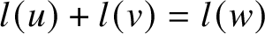 $l(u)+l(v)=l(w)$
we get
$l(u)+l(v)=l(w)$
we get
 $$ \begin{align*} \mathsf{B}_+w\mathsf{B}_+=\mathsf{B}_+u\mathsf{B}_+v\mathsf{B}_+. \end{align*} $$
Therefore, if
![]() , then
, then
![]() . Conversely, if
. Conversely, if
![]() , then there exists a flag
, then there exists a flag
 $\mathsf {B}'$
such that
$\mathsf {B}'$
such that
![]() . Itremains to show the uniqueness of
. Itremains to show the uniqueness of
 $\mathsf {B}'$
.
$\mathsf {B}'$
.
Assume
 $v=s_i$
. Let
$v=s_i$
. Let
 $\mathsf {B}'''$
satisfy
$\mathsf {B}'''$
satisfy
![]() . Note that
. Note that
 $\mathsf {B}_+s_i\mathsf {B}_+s_i\mathsf {B}_+=\mathsf {B}_+\sqcup \mathsf {B}_+s_i\mathsf {B}_+$
. If
$\mathsf {B}_+s_i\mathsf {B}_+s_i\mathsf {B}_+=\mathsf {B}_+\sqcup \mathsf {B}_+s_i\mathsf {B}_+$
. If
 $\mathsf {B}'\neq \mathsf {B}'''$
, then we get
$\mathsf {B}'\neq \mathsf {B}'''$
, then we get
![]() . Putting all of the flags together, we get
. Putting all of the flags together, we get

Because
 $l(us_i)=l(u)+1$
, from the red arrows we get
$l(us_i)=l(u)+1$
, from the red arrows we get
![]() , which contradicts with the blue arrow
, which contradicts with the blue arrow
![]() . Therefore,
. Therefore,
 $\mathsf {B}'=\mathsf {B}'''$
. For general v, we first fix a reduced word
$\mathsf {B}'=\mathsf {B}'''$
. For general v, we first fix a reduced word
 $v=s_{i_1}s_{i_2} \dots s_{i_l}$
. By the above discussion, there is a unique
$v=s_{i_1}s_{i_2} \dots s_{i_l}$
. By the above discussion, there is a unique
 $\mathsf {B}'''$
such that
$\mathsf {B}'''$
such that
 . Then we focus on
 . The uniqueness of
 $\mathsf {B}'$
follows by induction on the length of v.
$\mathsf {B}'$
follows by induction on the length of v.
For the third case, using the second condition of twin Tits system recursively, we get
 $$ \begin{align*} \mathsf{B}_-u\mathsf{B}_+=\mathsf{B}_-w\mathsf{B}_+v^{-1}\mathsf{B}_+. \end{align*} $$
Therefore, if
 , then
![]() . Conversely, if
. Conversely, if
![]() , then there exists a
, then there exists a
 $\mathsf {B}^{-1}$
such that
$\mathsf {B}^{-1}$
such that
 . The uniqueness of
 $\mathsf {B}^{-1}$
follows from the same inductive method as in the proof of the first.
$\mathsf {B}^{-1}$
follows from the same inductive method as in the proof of the first.
All other cases are analogous to the third case.
Next let us investigate the space of flags that are of Tits distance
 $s_i$
from a fixed flag.
$s_i$
from a fixed flag.
Lemma A.6. If
![]() , then
, then
 $\mathsf {B}=e_i(q)\overline {s}_i\mathsf {B}_+$
for some
$\mathsf {B}=e_i(q)\overline {s}_i\mathsf {B}_+$
for some
 $q\in \mathbb {A}^1$
.
$q\in \mathbb {A}^1$
.
Proof. The space of flags of Tits distance
 $s_i$
to
$s_i$
to
 $\mathsf {B}_+$
is the quotient
$\mathsf {B}_+$
is the quotient
 $\left .\left (\mathsf {B}_+s_i\mathsf {B}_+\right )\right /\mathsf {B}_+$
. By Lemma 6.1.3 of [Reference KumarKum02], we get
$\left .\left (\mathsf {B}_+s_i\mathsf {B}_+\right )\right /\mathsf {B}_+$
. By Lemma 6.1.3 of [Reference KumarKum02], we get
 $\mathsf {B}_+=\mathsf {U}_i\mathsf {Q}_i$
, where the subgroup
$\mathsf {B}_+=\mathsf {U}_i\mathsf {Q}_i$
, where the subgroup
 $\mathsf {Q}_i=\mathsf {B}_+\cap {s}_i\mathsf {B}_+s_i$
. Therefore,
$\mathsf {Q}_i=\mathsf {B}_+\cap {s}_i\mathsf {B}_+s_i$
. Therefore,
 $$ \begin{align*} \left.\left(\mathsf{B}_+s_i\mathsf{B}_+\right)\right/\mathsf{B}_+=\left.\left(\mathsf{U}_i\mathsf{Q}_is_i\mathsf{B}_+\right)\right/\mathsf{B}_+=\left.\left(\mathsf{U}_is_i\mathsf{Q}_i\mathsf{B}_+\right)\right/\mathsf{B}_+=\left.\left(\mathsf{U}_is_i\mathsf{B}_+\right)\right/\mathsf{B}_+=\left\{e_i(q)\overline{s}_i\mathsf{B}_+\right\}.\\[-38pt] \end{align*} $$
Corollary A.7. Let
 $\mathsf {B}$
be in either
$\mathsf {B}$
be in either
 $\mathcal {B}_+$
or
$\mathcal {B}_+$
or
 $\mathcal {B}_-$
. The space of flags of Tits distance
$\mathcal {B}_-$
. The space of flags of Tits distance
 $s_i$
away from
$s_i$
away from
 $\mathsf {B}$
is isomorphic to
$\mathsf {B}$
is isomorphic to
 $\mathbb {A}^1$
.
$\mathbb {A}^1$
.
Proposition A.8. Let
 $u, v\in \mathsf {W}$
and let
$u, v\in \mathsf {W}$
and let
 $s_i$
be a simple reflection. Fix a pair
$s_i$
be a simple reflection. Fix a pair
![]() . Then the space of flags
. Then the space of flags
 $\mathsf {B}$
that fits into either of the triangles
$\mathsf {B}$
that fits into either of the triangles

is isomorphic to
 $$ \begin{align*} \left\{\begin{array}{ll} \mathbb{A}^1 & \text{if}\ v=s_iu\ \text{and}\ l\left(s_iu\right)<l(u), \\ \mathbb{G}_m & \text{if}\ v=u\ \text{and}\ l\left(s_iu\right)>l(u), \\ \{*\} & \text{if}\ v=s_iu\ \text{and}\ l\left(s_iu\right)>l(u),\\ \emptyset & \text{otherwise.} \end{array}\right. \end{align*} $$
Proof. By symmetry, we will only prove the first case. Without loss of generality, let
 $\mathsf {B}^0=u\mathsf {B}_+$
and
$\mathsf {B}^0=u\mathsf {B}_+$
and
 $\mathsf {B}_0=\mathsf {B}_-$
. The set of flags of Tits distance
$\mathsf {B}_0=\mathsf {B}_-$
. The set of flags of Tits distance
 $s_i$
to
$s_i$
to
 $\mathsf {B}_-$
is
$\mathsf {B}_-$
is
 $$ \begin{align} \left\{\mathsf{B}_-e_i(p) \mid p\in \mathbb{G}_m \right\} \sqcup \left\{ \mathsf{B}_-s_i\right\}. \end{align} $$
If
 $l\left (s_iu\right )< l(u)$
, then we obtain the the first case by Lemma 2.5 and Corollary A.7.
$l\left (s_iu\right )< l(u)$
, then we obtain the the first case by Lemma 2.5 and Corollary A.7.
If
 $l\left (s_iu\right )> l(u)$
, then the root
$l\left (s_iu\right )> l(u)$
, then the root
 $\alpha :=u^{-1}\left (\alpha _i\right )$
is positive. Therefore,
$\alpha :=u^{-1}\left (\alpha _i\right )$
is positive. Therefore,
 $$ \begin{align*} \mathsf{B}_-e_i(p)u\mathsf{B}_+= \mathsf{B}_-u e_\alpha(p')\mathsf{B}_+ = \mathsf{B}_- u \mathsf{B}_+. \end{align*} $$
Among all of the flags in (A.9), only
 $\mathsf {B}_-s_i$
is of Tits codistance
$\mathsf {B}_-s_i$
is of Tits codistance
 $s_iu$
away from
$s_iu$
away from
 $\mathsf {B}_-u$
, from which we arrive at the third case. The rest are of Tits codistance u, which proves the second case.
$\mathsf {B}_-u$
, from which we arrive at the third case. The rest are of Tits codistance u, which proves the second case.
Now let us focus on
 $\mathsf {G}_{\mathrm {sc}}$
. Let
$\mathsf {G}_{\mathrm {sc}}$
. Let
 $V_\lambda $
denote the irreducible representation of
$V_\lambda $
denote the irreducible representation of
 $\mathsf {G}_{\mathrm {sc}}$
of highest weight
$\mathsf {G}_{\mathrm {sc}}$
of highest weight
 $\lambda \in \mathsf {P}_+$
. Let
$\lambda \in \mathsf {P}_+$
. Let
 $\mathcal {O}\left [\mathsf {G}_{\mathrm {sc}}\right ]$
be the algebra generated by the matrix coefficients of
$\mathcal {O}\left [\mathsf {G}_{\mathrm {sc}}\right ]$
be the algebra generated by the matrix coefficients of
 $V_\lambda $
,
$V_\lambda $
,
 $\lambda \in \mathsf {P}_+$
.
$\lambda \in \mathsf {P}_+$
.
Theorem A.10 Kac–Peterson, [Reference Kac and PetersonKP83, Theorem 1]
Consider the
 $\mathsf {G}_{\mathrm {sc}}\times \mathsf {G}_{\mathrm {sc}}$
-action on
$\mathsf {G}_{\mathrm {sc}}\times \mathsf {G}_{\mathrm {sc}}$
-action on
 $\mathcal {O}\left [\mathsf {G}_{\mathrm {sc}}\right ]$
by
$\mathcal {O}\left [\mathsf {G}_{\mathrm {sc}}\right ]$
by
 $$ \begin{align*}\left(\left(g_1,g_2\right).f\right)(g):=f\left(g_1^{-1}gg_2\right). \end{align*} $$
Then as
 $\mathsf {G}_{\mathrm {sc}}\times \mathsf {G}_{\mathrm {sc}}$
-modules,
$\mathsf {G}_{\mathrm {sc}}\times \mathsf {G}_{\mathrm {sc}}$
-modules,
 $$ \begin{align*}\mathcal{O}\left[\mathsf{G}_{\mathrm{sc}}\right]\cong \bigoplus_{\lambda\in \mathsf{P}_+}V^*_\lambda\otimes V_\lambda. \end{align*} $$
Let
 $^{\mathsf {U}_-}\mathcal {O}\left [\mathsf {G}_{\mathrm {sc}}\right ]$
be the subring of left
$^{\mathsf {U}_-}\mathcal {O}\left [\mathsf {G}_{\mathrm {sc}}\right ]$
be the subring of left
 $\mathsf {U}_-$
invariant functions. By Theorem A.10, we get
$\mathsf {U}_-$
invariant functions. By Theorem A.10, we get
 $$ \begin{align*}^{\mathsf{U}_-}\mathcal{O}\left[\mathsf{G}_{\mathrm{sc}}\right]\cong \bigoplus_{\lambda\in \mathsf{P}_+}V_\lambda.\end{align*} $$
Let
 $\Delta _\lambda \in V_\lambda $
be the unique highest weight vector such that
$\Delta _\lambda \in V_\lambda $
be the unique highest weight vector such that
 $\Delta _\lambda (e)=1$
. Given
$\Delta _\lambda (e)=1$
. Given
 $\lambda , \mu \in \mathsf {P}_+$
, the product
$\lambda , \mu \in \mathsf {P}_+$
, the product
 $\Delta _\lambda \Delta _\mu $
is a highest weight vector in
$\Delta _\lambda \Delta _\mu $
is a highest weight vector in
 $V_{\lambda +\mu }$
and satisfies the normalisation condition. Therefore,
$V_{\lambda +\mu }$
and satisfies the normalisation condition. Therefore,
 $$ \begin{align*} \Delta_{\lambda+\mu}=\Delta_\lambda\Delta_\mu. \end{align*} $$
Theorem A.11 Geiss–Leclerc–Schröer [Reference Geiß, Leclerc and SchröerGLS11], 7.2
An element
 $x\in \mathsf {G}_{\mathrm {sc}}$
is Gaussian decomposable if and only if
$x\in \mathsf {G}_{\mathrm {sc}}$
is Gaussian decomposable if and only if
 $\Delta _{\omega _i}\left (x\right )\neq 0$
for all fundamental weights
$\Delta _{\omega _i}\left (x\right )\neq 0$
for all fundamental weights
 $\omega _i$
.
$\omega _i$
.
A.2 Basics about Cluster Algebras
We include here the basic facts about cluster algebras that will be needed.
Definition A.12. A seed is a quadruple
 $\mathbf {s}=\left (I, I^{\mathrm {uf}}, \epsilon _{ab}, \left \{d_a\right \}_{a\in I}\right )$
satisfying the following properties:
$\mathbf {s}=\left (I, I^{\mathrm {uf}}, \epsilon _{ab}, \left \{d_a\right \}_{a\in I}\right )$
satisfying the following properties:
-
(1) I is a finite set and
$I^{\mathrm {uf}}\subset I$
; -
(2)
$\epsilon _{ab}$
is a
$\mathbb {Q}$
-valued matrix with
$\epsilon _{ab}\in \mathbb {Z}$
unless
$(a,b)\in I^{uf}\times I^{uf}$
; -
(3)
$\left \{d_a\right \}$
is a collection of positive integers with
$\gcd \left (d_a\right )=1$
such that the matrix
$ \hat {\epsilon }_{ab}:=\epsilon _{ab}d_b^{-1} $
is skew-symmetric.


Elements of I are called vertices, elements of
 $I^{\mathrm {uf}}$
are called unfrozen vertices and elements of
$I^{\mathrm {uf}}$
are called unfrozen vertices and elements of
 $I\setminus I^{\mathrm {uf}}$
are called frozen vertices. The matrix
$I\setminus I^{\mathrm {uf}}$
are called frozen vertices. The matrix
 $\epsilon $
is called the exchange matrix and
$\epsilon $
is called the exchange matrix and
 $d_a$
are called multipliers.
$d_a$
are called multipliers.
Definition A.13. Given a seed
 $\mathbf {s}$
and an unfrozen vertex
$\mathbf {s}$
and an unfrozen vertex
 $c\in I^{\mathrm {uf}}$
, a mutation at c produces a new seed
$c\in I^{\mathrm {uf}}$
, a mutation at c produces a new seed
 $\mathbf {s}'=\mu _c\mathbf {s}=\left (I', I^{\prime \mathrm {uf}}, \epsilon _{ab}', \{d^{\prime }_a\}\right )$
with
$\mathbf {s}'=\mu _c\mathbf {s}=\left (I', I^{\prime \mathrm {uf}}, \epsilon _{ab}', \{d^{\prime }_a\}\right )$
with
 $I'=I$
,
$I'=I$
,
 $I^{\prime \mathrm {uf}}=I^{\mathrm {uf}}$
,
$I^{\prime \mathrm {uf}}=I^{\mathrm {uf}}$
,
 $d^{\prime }_a=d_a$
and
$d^{\prime }_a=d_a$
and
 $$ \begin{align*} \epsilon^{\prime}_{ab}=\left\{\begin{array}{ll} -\epsilon_{ab} & \text{if}\ c\in \{a,b\},\\ \epsilon_{ab}+\left[\epsilon_{ac}\right]_+\left[\epsilon_{cb}\right]_+-\left[-\epsilon_{ac}\right]_+\left[-\epsilon_{cb}\right]_+ & \text{if}\ c\notin\{a,b\},\end{array}\right. \end{align*} $$
where
 $[x]_+:=\max \{x,0\}$
. Seeds obtained by a sequence of mutations on
$[x]_+:=\max \{x,0\}$
. Seeds obtained by a sequence of mutations on
 $\mathbf {s}$
are said to be mutation equivalent to
$\mathbf {s}$
are said to be mutation equivalent to
 $\mathbf {s}$
.
$\mathbf {s}$
.
Let
 $\mathbb {T}$
be an
$\mathbb {T}$
be an
 $\left |I^{\mathrm {uf}}\right |$
-regular tree. The edges of
$\left |I^{\mathrm {uf}}\right |$
-regular tree. The edges of
 $\mathbb {T}$
are labelled by elements of
$\mathbb {T}$
are labelled by elements of
 $I^{\mathrm {uf}}$
such that the labelling of edges connecting to the same vertex are distinct. Every mutation is involutive:
$I^{\mathrm {uf}}$
such that the labelling of edges connecting to the same vertex are distinct. Every mutation is involutive:
 $\mu _c^2\mathbf {s}=\mathbf {s}$
. Therefore, we can associate the vertices of
$\mu _c^2\mathbf {s}=\mathbf {s}$
. Therefore, we can associate the vertices of
 $\mathbb {T}$
with seeds from a mutation equivalent family, such that any two vertices associated to a pair of seeds related by a mutation
$\mathbb {T}$
with seeds from a mutation equivalent family, such that any two vertices associated to a pair of seeds related by a mutation
 $\mu _c$
are joined by an edge labelled by c. The decorated tree
$\mu _c$
are joined by an edge labelled by c. The decorated tree
 $\mathbb {T}$
is called the mutation tree of
$\mathbb {T}$
is called the mutation tree of
 $\mathbf {s}$
.
$\mathbf {s}$
.
We assign to each vertex
 $\mathbf {s}$
of
$\mathbf {s}$
of
 $\mathbb {T}$
two split
$\mathbb {T}$
two split
 $|I|$
-dimensional algebraic tori: a
$|I|$
-dimensional algebraic tori: a
 $\mathrm {K}_2$
seed torus
$\mathrm {K}_2$
seed torus
 $T_{\mathscr {A};\mathbf {s}}$
and a Poisson seed torus
$T_{\mathscr {A};\mathbf {s}}$
and a Poisson seed torus
 $T_{\mathscr {X};\mathbf {s}}$
. The tori
$T_{\mathscr {X};\mathbf {s}}$
. The tori
 $T_{\mathscr {A};\mathbf {s}}$
and
$T_{\mathscr {A};\mathbf {s}}$
and
 $T_{\mathscr {X};\mathbf {s}}$
are equipped with coordinate systems
$T_{\mathscr {X};\mathbf {s}}$
are equipped with coordinate systems
 $\left \{A_{a;\mathbf {s}}\right \}_{a\in I}$
and
$\left \{A_{a;\mathbf {s}}\right \}_{a\in I}$
and
 $\left \{X_{a;\mathbf {s}}\right \}_{a\in I}$
, respectively. We often drop the subscript
$\left \{X_{a;\mathbf {s}}\right \}_{a\in I}$
, respectively. We often drop the subscript
 $;\mathbf {s}$
if it is obvious or not important. The torus
$;\mathbf {s}$
if it is obvious or not important. The torus
 $T_{\mathscr {A};\mathbf {s}}$
admits a canonical 2-form
$T_{\mathscr {A};\mathbf {s}}$
admits a canonical 2-form
 $$ \begin{align*} \Omega=\sum_{a,b}\hat{\epsilon}_{ab;\mathbf{s}} \frac{dA_{a;\mathbf{s}}}{A_{a;\mathbf{s}}}\wedge \frac{dA_{b;\mathbf{s}}}{A_{b;\mathbf{s}}}. \end{align*} $$
The torus
 $T_{\mathscr {X};\mathbf {s}}$
admits a canonical Poisson structure determined by the bivector field
$T_{\mathscr {X};\mathbf {s}}$
admits a canonical Poisson structure determined by the bivector field
 $$ \begin{align*} \Pi=\sum_{a,b}\hat{\epsilon}_{ab;\mathbf{s}}X_{a;\mathbf{s}}X_{b;\mathbf{s}}\frac{\partial}{\partial X_{a;\mathbf{s}}}\wedge \frac{\partial }{\partial X_{b;\mathbf{s}}}. \end{align*} $$
For every edge
![]() in
in
 $\mathbb {T}$
, the associated seed tori are related by the transition maps
$\mathbb {T}$
, the associated seed tori are related by the transition maps

In terms of the cluster coordinates, the transition maps are expressed as
 $$ \begin{align} \mu_c^*\left(A_{a;\mathbf{s}'}\right):=\left\{\begin{array}{ll} A_{c;\mathbf{s}}^{-1}\left(\prod_b A_{b;\mathbf{s}}^{\left[-\epsilon_{cb;\mathbf{s}}\right]_+}\right)\left(1+\prod_b A_{b;\mathbf{s}}^{\epsilon_{cb;\mathbf{s}}}\right) & \text{if}\ a=c,\\ A_{a;\mathbf{s}} & \text{if}\ a\neq c, \end{array}\right. \end{align} $$
 $$ \begin{align} \mu_c^*\left(X_{a;\mathbf{s}'}\right):=\left\{\begin{array}{ll} X_{c;\mathbf{s}}^{-1} & \text{if}\ a=c,\\ X_{a;\mathbf{s}}X_{c;\mathbf{s}}^{\left[\epsilon_{ac;\mathbf{s}}\right]_+}\left(1+X_{c;\mathbf{s}}\right)^{-\epsilon_{ac;\mathbf{s}}}& \text{if}\ a\neq c.\end{array}\right. \end{align} $$
The maps
 $\mu _c$
preserve the 2-form
$\mu _c$
preserve the 2-form
 $\Omega $
and the bivector field
$\Omega $
and the bivector field
 $\Pi $
.
$\Pi $
.
Let
 $\mathbf {s}$
and
$\mathbf {s}$
and
 $\mathbf {s}'$
be any two not necessarily adjacent vertices on
$\mathbf {s}'$
be any two not necessarily adjacent vertices on
 $\mathbb {T}$
. By composing the transition maps along the unique path connecting them, we get birational maps
$\mathbb {T}$
. By composing the transition maps along the unique path connecting them, we get birational maps
 $\mu _{\mathbf {s}\rightarrow \mathbf {s}'}:T_{\mathscr {A};\mathbf {s}}\dashrightarrow T_{\mathscr {A};\mathbf {s}'}$
and
$\mu _{\mathbf {s}\rightarrow \mathbf {s}'}:T_{\mathscr {A};\mathbf {s}}\dashrightarrow T_{\mathscr {A};\mathbf {s}'}$
and
 $\mu _{\mathbf {s}\rightarrow \mathbf {s}'}:T_{\mathscr {X};\mathbf {s}}\dashrightarrow T_{\mathscr {X};\mathbf {s}'}$
. Fomin and Zelevinsky [Reference Fomin and ZelevinskyFZ07] proved the following factorisation formulas for the pullbacks of cluster coordinates:
$\mu _{\mathbf {s}\rightarrow \mathbf {s}'}:T_{\mathscr {X};\mathbf {s}}\dashrightarrow T_{\mathscr {X};\mathbf {s}'}$
. Fomin and Zelevinsky [Reference Fomin and ZelevinskyFZ07] proved the following factorisation formulas for the pullbacks of cluster coordinates:
 $$ \begin{align} \mu_{\mathbf{s}\rightarrow \mathbf{s}'}^*\left(A_{a;\mathbf{s}'}\right)=&\left(\prod_b A_{b;\mathbf{s}}^{g_{ab;\mathbf{s}\rightarrow \mathbf{s}'}}\right)\left(\left.F_{a;\mathbf{s}\rightarrow \mathbf{s}'}\right|{}_{X_{b;\mathbf{s}}=\prod_cA_{c;\mathbf{s}}^{\epsilon_{bc;\mathbf{s}}}}\right), \end{align} $$
 $$ \begin{align} \mu_{\mathbf{s}\rightarrow \mathbf{s}'}^*\left(X_{a;\mathbf{s}'}\right)=&\left(\prod_b X_{b;\mathbf{s}}^{c_{ab;\mathbf{s}\rightarrow \mathbf{s}'}}\right)\left(\prod_b \left(F_{b;\mathbf{s}\rightarrow \mathbf{s}'}\right)^{\epsilon_{ab;\mathbf{s}'}}\right), \end{align} $$
where
 $c_{ab;\mathbf {s}\rightarrow \mathbf {s}'}$
and
$c_{ab;\mathbf {s}\rightarrow \mathbf {s}'}$
and
 $g_{ab;\mathbf {s}\rightarrow \mathbf {s}'}$
are
$g_{ab;\mathbf {s}\rightarrow \mathbf {s}'}$
are
 $I\times I$
matrices with integer entries and
$I\times I$
matrices with integer entries and
 $F_{a;\mathbf {s}\rightarrow \mathbf {s}'}$
are polynomials in the initial cluster Poisson coordinates
$F_{a;\mathbf {s}\rightarrow \mathbf {s}'}$
are polynomials in the initial cluster Poisson coordinates
 $\left \{X_{a;\mathbf {s}}\right \}$
. They are called the c-matrix, the g-matrix and the F-polynomials associated to the mutation map
$\left \{X_{a;\mathbf {s}}\right \}$
. They are called the c-matrix, the g-matrix and the F-polynomials associated to the mutation map
 $\mu _{\mathbf {s}\rightarrow \mathbf {s}'}$
, respectively. We have the following properties:
$\mu _{\mathbf {s}\rightarrow \mathbf {s}'}$
, respectively. We have the following properties:
-
(1) (matrix identities)
$\epsilon _{;\mathbf {s}'}g_{;\mathbf {s}\rightarrow \mathbf {s}'}=c_{;\mathbf {s}\rightarrow \mathbf {s}'}\epsilon _{;\mathbf {s}}$
; -
(2) (sign coherence) row vectors of c-matrices and column vectors of g-matrices are sign coherent; that is, their entries are either all nonnegative or all nonpositive;
-
(3) (constant term) F-polynomials all have a constant term 1;
-
(4) (positivity) F-polynomials all have positive integer coefficients.

In addition, the following properties are immediate consequences of the factorisation formulas:
-
(5) (Laurent phenomenon)
$\mu _{\mathbf {s}\rightarrow \mathbf {s}'}\left (A_{a;\mathbf {s}'}\right )$
is a Laurent polynomial; -
(6)
$c_{ab;\mathbf {s}\rightarrow \mathbf {s}'}=\mathrm {ord}_{X_{b;\mathbf {s}}}\mu _{\mathbf {s}\rightarrow \mathbf {s}'}^*\left (X_{a;\mathbf {s}'}\right )$
, where
$\mathrm {ord}_xf$
yields the lowest degree of x in f if f is a polynomial and
$\mathrm {ord}_x\left (\frac {f}{g}\right ):=\mathrm {ord}_xf-\mathrm {ord}_xg$
.


Let us fix an initial seed
 $\mathbf {s}$
. The sign coherence of c-vectors allows us to assign a colour to each vertex
$\mathbf {s}$
. The sign coherence of c-vectors allows us to assign a colour to each vertex
 $a\in I$
in a seed
$a\in I$
in a seed
 $\mathbf {s}'$
: we say a is green if
$\mathbf {s}'$
: we say a is green if
 $c_{ab;\mathbf {s}\rightarrow \mathbf {s}'}\geq 0$
for all b and red otherwise. Note that a mutation at the vertex c changes its colour, but it may change the colours of other vertices as well.
$c_{ab;\mathbf {s}\rightarrow \mathbf {s}'}\geq 0$
for all b and red otherwise. Note that a mutation at the vertex c changes its colour, but it may change the colours of other vertices as well.
From the above definition, all vertices of the initial seed
 $\mathbf {s}$
are green. A sequence of mutations that turns all vertices red is called a reddening sequence and a reddening sequence consisting of mutations only in the direction of green vertices is called a maximal green sequence.
$\mathbf {s}$
are green. A sequence of mutations that turns all vertices red is called a reddening sequence and a reddening sequence consisting of mutations only in the direction of green vertices is called a maximal green sequence.
There is a combinatorial way to compute the c-matrix using principal coefficients. Given a seed
 $\mathbf {s}=\left (I, I^{\mathrm {uf}}, \epsilon _{;\mathbf {s}}, \left \{d_a\right \}\right )$
, we define the corresponding seed with principal coefficients as
$\mathbf {s}=\left (I, I^{\mathrm {uf}}, \epsilon _{;\mathbf {s}}, \left \{d_a\right \}\right )$
, we define the corresponding seed with principal coefficients as
 $$ \begin{align*} \mathbf{s}_{\mathrm{prin}}=\left(I\sqcup I, I^{\mathrm{uf}}\sqcup \emptyset, \begin{pmatrix} \epsilon_{;\mathbf{s}} & \mathrm{id} \\ -\mathrm{id} & 0 \end{pmatrix}, \left\{d_a\right\}\sqcup \left\{d_a\right\}\right). \end{align*} $$
By applying the sequence of mutations
 $\mu _{\mathbf {s}\rightarrow \mathbf {s}'}$
to
$\mu _{\mathbf {s}\rightarrow \mathbf {s}'}$
to
 $\mathbf {s}_{\mathrm {prin}}$
, we obtain a seed with exchange matrix
$\mathbf {s}_{\mathrm {prin}}$
, we obtain a seed with exchange matrix
 $\begin {pmatrix}\epsilon _{;\mathbf {s}'} & c_{;\mathbf {s}\rightarrow \mathbf {s}'} \\ * & *\end {pmatrix}$
, whose upper right-hand corner is precisely the c-matrix we need.
$\begin {pmatrix}\epsilon _{;\mathbf {s}'} & c_{;\mathbf {s}\rightarrow \mathbf {s}'} \\ * & *\end {pmatrix}$
, whose upper right-hand corner is precisely the c-matrix we need.
Definition A.18. Fix an initial seed
 $\mathbf {s}$
in
$\mathbf {s}$
in
 $\mathbb {T}$
. We define the upper cluster algebra to be
$\mathbb {T}$
. We define the upper cluster algebra to be
 $$ \begin{align*} \mathrm{up} \left(\mathscr{A}\right):=\bigcap_{\mathbf{s'}}\mu_{\mathbf{s}\rightarrow \mathbf{s'}}^*\left(\mathcal{O}\left(T_{\mathscr{A};\mathbf{s'}}\right)\right)\subset \mathrm{Frac} \left(\mathcal{O}\left(T_{\mathscr{A};\mathbf{s}}\right)\right) \end{align*} $$
and define the cluster Poisson algebra to be
 $$ \begin{align*} \mathrm{up} \left(\mathscr{X}\right):=\bigcap_{\mathbf{s}}\mu_{\mathbf{s}\rightarrow \mathbf{s'}}^*\left(\mathcal{O}\left(T_{\mathscr{X};\mathbf{s'}}\right)\right)\subset \mathrm{Frac} \left(\mathcal{O}\left(T_{\mathscr{X};\mathbf{s}}\right)\right). \end{align*} $$
Note that
 $\mathcal {O}\left (T_{\mathscr {X};\mathbf {s'}}\right )$
is a Poisson algebra for each seed
$\mathcal {O}\left (T_{\mathscr {X};\mathbf {s'}}\right )$
is a Poisson algebra for each seed
 $\mathbf {s'}$
and the mutation maps preserve the Poisson structure. Therefore,
$\mathbf {s'}$
and the mutation maps preserve the Poisson structure. Therefore,
 $\mathrm {up}\left (\mathscr {X}\right )$
is naturally a Poisson algebra.
$\mathrm {up}\left (\mathscr {X}\right )$
is naturally a Poisson algebra.
The algebras
 $\mathrm {up} \left (\mathscr {A}\right )$
and
$\mathrm {up} \left (\mathscr {A}\right )$
and
 $\mathrm {up} \left (\mathscr {X}\right )$
do not depend on the choice of an initial seed, because all mutation maps are algebra isomorphisms on the fields of fractions and
$\mathrm {up} \left (\mathscr {X}\right )$
do not depend on the choice of an initial seed, because all mutation maps are algebra isomorphisms on the fields of fractions and
 $\mu _c^2=\mathrm {id}$
.
$\mu _c^2=\mathrm {id}$
.
Definition A.19. The geometric counterparts of
 $\mathrm {up}(\mathscr {A})$
and
$\mathrm {up}(\mathscr {A})$
and
 $\mathrm {up}(\mathscr {X})$
are the cluster
$\mathrm {up}(\mathscr {X})$
are the cluster
 $\mathrm {K}_2$
variety
$\mathrm {K}_2$
variety
 $\mathscr {A}$
and the cluster Poisson variety
Footnote
8
$\mathscr {A}$
and the cluster Poisson variety
Footnote
8
 $\mathscr {X}$
, obtained by gluing the seed tori via the transition maps
$\mathscr {X}$
, obtained by gluing the seed tori via the transition maps
 $\mu $
:
$\mu $
:
 $$ \begin{align*} \mathscr{A}=\left.\bigsqcup_{\mathbf{s}} T_{\mathscr{A};\mathbf{s}}\right/\left\{\mu_c\right\} \quad \text{and} \quad \mathscr{X}=\left.\bigsqcup_{\mathbf{s}} T_{\mathscr{X};\mathbf{s}}\right/\left\{\mu_c\right\}. \end{align*} $$
In particular,
 $\mathcal {O}(\mathscr {A})= \mathrm {up}(\mathscr {A})$
and
$\mathcal {O}(\mathscr {A})= \mathrm {up}(\mathscr {A})$
and
 $\mathcal {O}(\mathscr {X})=\mathrm {up}(\mathscr {X})$
.
$\mathcal {O}(\mathscr {X})=\mathrm {up}(\mathscr {X})$
.
Because the mutation maps between
 $T_{\mathscr {A};\mathbf {s}}$
preserve the canonical 2-forms
$T_{\mathscr {A};\mathbf {s}}$
preserve the canonical 2-forms
 $\Omega $
, these 2-forms can be glued into a canonical 2-form
$\Omega $
, these 2-forms can be glued into a canonical 2-form
 $\Omega $
on the cluster
$\Omega $
on the cluster
 $\mathrm {K}_2$
variety
$\mathrm {K}_2$
variety
 $\mathscr {A}$
. Similarly, because the mutation maps between
$\mathscr {A}$
. Similarly, because the mutation maps between
 $T_{\mathscr {X};\mathbf {s}}$
are Poisson maps, the cluster Poisson variety
$T_{\mathscr {X};\mathbf {s}}$
are Poisson maps, the cluster Poisson variety
 $\mathscr {X}$
is naturally a Poisson variety.
$\mathscr {X}$
is naturally a Poisson variety.
Definition A.20. Let
 $\mathbf {s}$
and
$\mathbf {s}$
and
 $\mathbf {s}'$
be two seeds on
$\mathbf {s}'$
be two seeds on
 $\mathbb {T}$
. A seed isomorphism
$\mathbb {T}$
. A seed isomorphism
 $\sigma ^*:\mathbf {s}\rightarrow \mathbf {s}'$
is a bijection
$\sigma ^*:\mathbf {s}\rightarrow \mathbf {s}'$
is a bijection
 $\sigma ^*:I\rightarrow I$
such that
$\sigma ^*:I\rightarrow I$
such that
 $\sigma ^*\left (I^{\mathrm {uf}}\right )=I^{\mathrm {uf}}$
,
$\sigma ^*\left (I^{\mathrm {uf}}\right )=I^{\mathrm {uf}}$
,
 $d_a=d_{\sigma ^*(a)}$
and
$d_a=d_{\sigma ^*(a)}$
and
 $\epsilon _{ab;\mathbf {s}}=\epsilon _{\sigma ^*(a)\sigma ^*(b);\mathbf {s}'}$
.
$\epsilon _{ab;\mathbf {s}}=\epsilon _{\sigma ^*(a)\sigma ^*(b);\mathbf {s}'}$
.
Definition A.21. A seed isomorphism
 $\sigma ^*:\mathbf {s}\rightarrow \mathbf {s}'$
induces algebra automorphisms
$\sigma ^*:\mathbf {s}\rightarrow \mathbf {s}'$
induces algebra automorphisms
 $\sigma ^*$
on
$\sigma ^*$
on
 $\mathrm {up}(\mathscr {A})$
and
$\mathrm {up}(\mathscr {A})$
and
 $\mathrm {up}(\mathscr {X})$
defined by
$\mathrm {up}(\mathscr {X})$
defined by
 $$ \begin{align*} \sigma^*\left(A_{a;\mathbf{s}}\right):=A_{\sigma^*(a);\mathbf{s}'} \quad \text{and} \quad \sigma^*\left(X_{a;\mathbf{s}}\right):=X_{\sigma^*(a);\mathbf{s}'}. \end{align*} $$
Abusing notation, we still denote by
 $\sigma $
the induced biregular automorphisms of the corresponding cluster varieties. Such automorphisms are called cluster transformations.
$\sigma $
the induced biregular automorphisms of the corresponding cluster varieties. Such automorphisms are called cluster transformations.
A cluster transformation pulls back cluster variables to cluster variables according to the factorisation formulas (A.16) and (A.17). Therefore. it makes sense to define the c-matrix, the g-matrix and the F-polynomials of a cluster transformation
 $\sigma $
with respect to a choice of initial seed
$\sigma $
with respect to a choice of initial seed
 $\mathbf {s}$
; we denote them by
$\mathbf {s}$
; we denote them by
 $c_{;\sigma ;\mathbf {s}}$
,
$c_{;\sigma ;\mathbf {s}}$
,
 $g_{;\sigma ;\mathbf {s}}$
and
$g_{;\sigma ;\mathbf {s}}$
and
 $F_{;\sigma ;\mathbf {s}}$
. respectively.
$F_{;\sigma ;\mathbf {s}}$
. respectively.
The following criteria determine when a cluster transformation is trivial.
Theorem A.22 [Reference Goncharov and ShenGS18, Reference Gross, Hacking, Keel and KontsevichGHKK18, Reference Cao, Huang and LiCHL18]
Let
 $\sigma $
be a cluster transformation on
$\sigma $
be a cluster transformation on
 $\mathscr {A}$
and
$\mathscr {A}$
and
 $\mathscr {X}$
. The following statements are equivalent:
$\mathscr {X}$
. The following statements are equivalent:
-
•
$\sigma $
acts trivially on
$\mathscr {A}$
; -
•
$\sigma $
acts trivially on
$\mathscr {X}$
; -
• the c-matrix with respect to one (and equivalently any) seed is the identity matrix;
-
• the g-matrix with respect to one (and equivalently any) seed is the identity matrix.


By Theorem A.22, the group of cluster transformations on
 $\mathscr {A}$
coincides with the group of cluster transformations on
$\mathscr {A}$
coincides with the group of cluster transformations on
 $\mathscr {X}$
. We call this group the cluster modular group and denote it by
$\mathscr {X}$
. We call this group the cluster modular group and denote it by
 $\mathscr {G}$
.
$\mathscr {G}$
.
Definition A.23. Fix a seed
 $\mathbf {s}=\left (I,I^{\mathrm {uf}},\epsilon _{ab},\left \{d_a\right \}\right )$
. Let
$\mathbf {s}=\left (I,I^{\mathrm {uf}},\epsilon _{ab},\left \{d_a\right \}\right )$
. Let
 $d=\mathrm {lcm}\left \{d_a\right \}$
. We define the Langlands dual seed
$d=\mathrm {lcm}\left \{d_a\right \}$
. We define the Langlands dual seed
 $\mathbf {s}^\vee :=\left (I,I^{\mathrm {uf}}, -\epsilon _{ba}, \left \{d/d_a\right \}\right )$
and the chiral dual seed
$\mathbf {s}^\vee :=\left (I,I^{\mathrm {uf}}, -\epsilon _{ba}, \left \{d/d_a\right \}\right )$
and the chiral dual seed
 $\mathbf {s}^\circ :=\left (I,I^{\mathrm {uf}},-\epsilon _{ab},\left \{d_a\right \}\right )$
.
$\mathbf {s}^\circ :=\left (I,I^{\mathrm {uf}},-\epsilon _{ab},\left \{d_a\right \}\right )$
.
The following facts are easy to check:
-
(a)
$\mathbf {s}^{\vee \vee }=\mathbf {s}$
and
$\mathbf {s}^{\circ \circ }=\mathbf {s}$
; -
(b)
$\mu _c\mathbf {s}^\vee =\left (\mu _c\mathbf {s}\right )^\vee $
and
$\mu _c\mathbf {s}^\circ =\left (\mu _c\mathbf {s}\right )^\circ $
; -
(c) the following are equivalent for a bijection
$\sigma ^*:I\rightarrow I$
:-
•
$\sigma ^*:\mathbf {s}\rightarrow \mathbf {s}'$
is a seed isomorphism; -
•
$\sigma ^*:\mathbf {s}^\vee \rightarrow \mathbf {s}^{\prime \vee }$
is a seed isomorphism; -
•
$\sigma ^*:\mathbf {s}^\circ \rightarrow \mathbf {s}^{\prime \circ }$
is a seed isomorphism.
-


Thanks to (b), the mutation trees of
 $\mathbf {s}$
,
$\mathbf {s}$
,
 $\mathbf {s}^\vee $
and
$\mathbf {s}^\vee $
and
 $\mathbf {s}^\circ $
are naturally isomorphic. We can define the Langlands dual versions and chiral dual versions of cluster algebras and cluster varieties the same way as before and we will denote them with superscripts
$\mathbf {s}^\circ $
are naturally isomorphic. We can define the Langlands dual versions and chiral dual versions of cluster algebras and cluster varieties the same way as before and we will denote them with superscripts
 $^\vee $
and
$^\vee $
and
 $^\circ $
, respectively. Nakanishi and Zelevinsky [Reference Nakanishi and ZelevinskyNZ12] proved the following tropical duality relating the c-matrix and g-matrix associated to the same sequence of mutations when applied to Langlands dual seeds:
$^\circ $
, respectively. Nakanishi and Zelevinsky [Reference Nakanishi and ZelevinskyNZ12] proved the following tropical duality relating the c-matrix and g-matrix associated to the same sequence of mutations when applied to Langlands dual seeds:
 $$ \begin{align} c_{;\mathbf{s}\rightarrow \mathbf{s}'}^t=g_{;\mathbf{s}^\vee\rightarrow \mathbf{s}^{\prime \vee}}^{-1}; \end{align} $$
they also proved the following identity relating the c-matrices associated to the opposite sequence of mutations when applied to chiral dual seeds:
 $$ \begin{align} c_{;\mathbf{s}\rightarrow \mathbf{s}'}^{-1}=c_{;\mathbf{s}^{\prime \circ}\rightarrow \mathbf{s}^\circ}. \end{align} $$
It follows from (c) and the tropical duality that a cluster transformation is trivial if and only if the corresponding cluster transformation on the Langlands dual (respectively chiral dual) is trivial. Thus, the Langlands dual (respectively chiral dual) cluster modular groups are isomorphic; that is,
 $\mathscr {G}\cong \mathscr {G}^\vee \cong \mathscr {G}^\circ $
.
$\mathscr {G}\cong \mathscr {G}^\vee \cong \mathscr {G}^\circ $
.
Cluster varieties
 $\mathscr {A}$
and
$\mathscr {A}$
and
 $\mathscr {X}$
are positive spaces; that is, they are equipped with a semifield of positive rational functions
$\mathscr {X}$
are positive spaces; that is, they are equipped with a semifield of positive rational functions
 $\mathbb {Q}_+(\mathscr {A})$
and
$\mathbb {Q}_+(\mathscr {A})$
and
 $\mathbb {Q}_+(\mathscr {X})$
, respectively. Given a semifield S, we define the set of S-points
$\mathbb {Q}_+(\mathscr {X})$
, respectively. Given a semifield S, we define the set of S-points
 $$ \begin{align*} \mathscr{A}(S):=\mathrm{Hom}_{\text{semifield}}\left(\mathbb{Q}_+(\mathscr{A}),S\right), \hskip 10mm \mathscr{X}(S):=\mathrm{Hom}_{\text{semifield}}\left(\mathbb{Q}_+(\mathscr{X}),S\right). \end{align*} $$
Let
 $\mathbb {Z}^t=(\mathbb {Z}, \min , +)$
be the semifield of tropical integers. Fock and Goncharov proposed the following conjecture on Langlands dual cluster varieties.
$\mathbb {Z}^t=(\mathbb {Z}, \min , +)$
be the semifield of tropical integers. Fock and Goncharov proposed the following conjecture on Langlands dual cluster varieties.
Conjecture A.26 [Reference Fock and GoncharovFG09a, Conj. 4.1]
The coordinate ring
 $\mathcal {O}(\mathscr {A})$
admits a basis
$\mathcal {O}(\mathscr {A})$
admits a basis
 $\mathscr {G}$
-equivariantly parametrised by
$\mathscr {G}$
-equivariantly parametrised by
 $\mathscr {X}^\vee \left (\mathbb {Z}^t\right )$
and
$\mathscr {X}^\vee \left (\mathbb {Z}^t\right )$
and
 $\mathcal {O}(\mathscr {X})$
admits a basis
$\mathcal {O}(\mathscr {X})$
admits a basis
 $\mathscr {G}$
-equivariantly parametrised by
$\mathscr {G}$
-equivariantly parametrised by
 $\mathscr {A}^\vee \left (\mathbb {Z}^t\right )$
.
$\mathscr {A}^\vee \left (\mathbb {Z}^t\right )$
.
Definition A.27. For a seed
 $\mathbf {s}=\left (I,I^{\mathrm {uf}},\epsilon ,\left \{d_a\right \}\right )$
with
$\mathbf {s}=\left (I,I^{\mathrm {uf}},\epsilon ,\left \{d_a\right \}\right )$
with
 $\gcd \left \{d_a\right \}_{a\in I^{\mathrm {uf}}}=1$
, we define its associated unfrozen seed to be
$\gcd \left \{d_a\right \}_{a\in I^{\mathrm {uf}}}=1$
, we define its associated unfrozen seed to be
 $\mathbf {s}^{\mathrm {uf}}=\left (I^{\mathrm {uf}}, I^{\mathrm {uf}}, \epsilon |_{I^{\mathrm {uf}}\times I^{\mathrm {uf}}}, \left \{d_a\right \}_{a\in I^{\mathrm {uf}}}\right )$
.
$\mathbf {s}^{\mathrm {uf}}=\left (I^{\mathrm {uf}}, I^{\mathrm {uf}}, \epsilon |_{I^{\mathrm {uf}}\times I^{\mathrm {uf}}}, \left \{d_a\right \}_{a\in I^{\mathrm {uf}}}\right )$
.
Let
 $\mathscr {A}^{\mathrm {uf}}$
and
$\mathscr {A}^{\mathrm {uf}}$
and
 $\mathscr {X}^{\mathrm {uf}}$
be the cluster varieties constructed from an unfrozen seed associated to a seed that defines
$\mathscr {X}^{\mathrm {uf}}$
be the cluster varieties constructed from an unfrozen seed associated to a seed that defines
 $\mathscr {A}$
and
$\mathscr {A}$
and
 $\mathscr {X}$
. Then among their seed tori we can define four maps
$\mathscr {X}$
. Then among their seed tori we can define four maps
 $$ \begin{align*} e:T_{\mathscr{A}^{\mathrm{uf}};\mathbf{s}^{\mathrm{uf}}} & \rightarrow T_{\mathscr{A};\mathbf{s}} & f:T_{\mathscr{A}^{\mathrm{uf}};\mathbf{s}^{\mathrm{uf}}}&\rightarrow T_{\mathscr{X};\mathbf{s}}\\ e^*\left(A_{a;\mathbf{s}}\right)&:=\left\{\begin{array}{ll} A_{a;\mathbf{s}^{\mathrm{uf}}} & \text{if}\ a\in I^{\mathrm{uf}},\\ 1 & \text{if}\ a\notin I^{\mathrm{uf}}, \end{array}\right. & f^*\left(X_{a;\mathbf{s}}\right)&:=\prod_{b\in I^{\mathrm{uf}}}A_{b;\mathbf{s}^{\mathrm{uf}}}^{\epsilon_{ab;\mathbf{s}}}\\ p:T_{\mathscr{A};\mathbf{s}}& \rightarrow T_{\mathscr{X}^{\mathrm{uf}};\mathbf{s}^{\mathrm{uf}}} & q:T_{\mathscr{X};\mathbf{s}}& \rightarrow T_{\mathscr{X}^{\mathrm{uf}};\mathbf{s}^{\mathrm{uf}}}\\ p^*\left(X_{a;\mathbf{s}^{\mathrm{uf}}}\right)&:=\prod_{b\in I}A_{b;\mathbf{s}}^{\epsilon_{ab;\mathbf{s}}} & q^*\left(X_{a;\mathbf{s}^{\mathrm{uf}}}\right)&:=X_{a;\mathbf{s}}. \end{align*} $$
By direct computation one can verify that these four maps commute with the mutation maps
 $\mu $
. Therefore, we can glue them together and obtain four regular maps in the following commutative diagram:
$\mu $
. Therefore, we can glue them together and obtain four regular maps in the following commutative diagram:

Let
 $\mathscr {G}$
be the cluster modular group associated to the cluster varieties
$\mathscr {G}$
be the cluster modular group associated to the cluster varieties
 $\mathscr {A}$
and
$\mathscr {A}$
and
 $\mathscr {X}$
and let
$\mathscr {X}$
and let
 $\mathscr {G}^{\mathrm {uf}}$
be the cluster modular group associated to the cluster varieties
$\mathscr {G}^{\mathrm {uf}}$
be the cluster modular group associated to the cluster varieties
 $\mathscr {A}^{\mathrm {uf}}$
and
$\mathscr {A}^{\mathrm {uf}}$
and
 $\mathscr {X}^{\mathrm {uf}}$
. It then follows from the above formulas that
$\mathscr {X}^{\mathrm {uf}}$
. It then follows from the above formulas that
 $\mathscr {G}$
is a subgroup of
$\mathscr {G}$
is a subgroup of
 $\mathscr {G}^{\mathrm {uf}}$
.
$\mathscr {G}^{\mathrm {uf}}$
.
Proposition A.28. Let
 $\pi :T_{\mathscr {A};\mathbf {s}}\rightarrow T_{\mathscr {X};\mathbf {s}}$
be a group homomorphism of algebraic tori for some fixed seed
$\pi :T_{\mathscr {A};\mathbf {s}}\rightarrow T_{\mathscr {X};\mathbf {s}}$
be a group homomorphism of algebraic tori for some fixed seed
 $\mathbf {s}$
such that
$\mathbf {s}$
such that
 $f=\pi \circ e$
and
$f=\pi \circ e$
and
 $p=q\circ \pi $
. Then
$p=q\circ \pi $
. Then
 $\pi $
induces group homomorphisms of algebraic tori between seed tori associated to any other seed in the mutation equivalent family. Moreover, they glue into a well-defined regular map
$\pi $
induces group homomorphisms of algebraic tori between seed tori associated to any other seed in the mutation equivalent family. Moreover, they glue into a well-defined regular map
 $\pi :\mathscr {A}\rightarrow \mathscr {X}$
.
$\pi :\mathscr {A}\rightarrow \mathscr {X}$
.
Proof. The conditions
 $p=\pi \circ e$
and
$p=\pi \circ e$
and
 $f=q\circ \pi $
imply that the only freedom in defining
$f=q\circ \pi $
imply that the only freedom in defining
 $\pi $
is the frozen factor (the first factor) in
$\pi $
is the frozen factor (the first factor) in
 $$ \begin{align*} \pi^*\left(X_{a;\mathbf{s}}\right):=\left(\prod_{b\in I\setminus I^{\mathrm{uf}}} A_{b;\mathbf{s}}^{\cdots} \right)\left(\prod_{c\in I^{\mathrm{uf}}}A_{c;\mathbf{s}}^{\epsilon_{ac;\mathbf{s}}}\right)=\left(\prod_{b\in I\setminus I^{\mathrm{uf}}} A_{b;\mathbf{s}}^{\cdots} \right)f^*\left(X_{a;\mathbf{s}}\right) \end{align*} $$
for each frozen vertex a. But such a factor need not change under mutation: we can just define
 $\pi ^*\left (X_{a;\mathbf {s}'}\right ):=\left (\prod _{b\in I\setminus I^{\mathrm {uf}}} A_{b;\mathbf {s}'}^{\cdots } \right )f^*\left (X_{a;\mathbf {s}'}\right )$
for any other seed
$\pi ^*\left (X_{a;\mathbf {s}'}\right ):=\left (\prod _{b\in I\setminus I^{\mathrm {uf}}} A_{b;\mathbf {s}'}^{\cdots } \right )f^*\left (X_{a;\mathbf {s}'}\right )$
for any other seed
 $\mathbf {s}'$
and such maps
$\mathbf {s}'$
and such maps
 $\pi $
automatically commute with the mutation maps.
$\pi $
automatically commute with the mutation maps.
Remark A.29. There is another way to describe the map
 $\pi $
. Let M and N be the character lattices of
$\pi $
. Let M and N be the character lattices of
 $T_{\mathscr {A};\mathbf {s}}$
and
$T_{\mathscr {A};\mathbf {s}}$
and
 $T_{\mathscr {X};\mathbf {s}}$
, respectively. Then
$T_{\mathscr {X};\mathbf {s}}$
, respectively. Then
 $\pi $
induces a linear map of character lattices
$\pi $
induces a linear map of character lattices
 $\pi ^*:N\rightarrow M$
. The cluster Poisson coordinates
$\pi ^*:N\rightarrow M$
. The cluster Poisson coordinates
 $\left \{X_{a;\mathbf {s}}\right \}$
correspond to a basis
$\left \{X_{a;\mathbf {s}}\right \}$
correspond to a basis
 $\left \{e_{a;\mathbf {s}}\right \}$
of N and the skew-symmetric matrix
$\left \{e_{a;\mathbf {s}}\right \}$
of N and the skew-symmetric matrix
 $\hat {\epsilon }_{ab}$
defines a skew-symmetric form
$\hat {\epsilon }_{ab}$
defines a skew-symmetric form
 $\{\cdot ,\cdot \}$
on N. We can view a seed mutation
$\{\cdot ,\cdot \}$
on N. We can view a seed mutation
 $\mathbf {s}'=\mu _c\mathbf {s}$
as a change of basis on the lattice N given by
$\mathbf {s}'=\mu _c\mathbf {s}$
as a change of basis on the lattice N given by
 $$ \begin{align*} e_{a;\mathbf{s}'}=\left\{\begin{array}{ll} -e_{c;\mathbf{s}} & \text{if}\ a=c, \\ e_{a;\mathbf{s}}+\left[\epsilon_{ac;\mathbf{s}}\right]_+e_{c;\mathbf{s}} & \text{if}\ a\neq c. \end{array}\right. \end{align*} $$
By viewing the seed tori
 $T_{\mathscr {A};\mathbf {s}'}$
and
$T_{\mathscr {A};\mathbf {s}'}$
and
 $T_{\mathscr {X};\mathbf {s}'}$
as algebraic tori with character lattices M and N, we can redefine the mutation map
$T_{\mathscr {X};\mathbf {s}'}$
as algebraic tori with character lattices M and N, we can redefine the mutation map
 $\mu _c$
between the corresponding seed tori by the following coordinate-free formula:
$\mu _c$
between the corresponding seed tori by the following coordinate-free formula:
 $$ \begin{align*} \mu_c^*\left(X^n\right)=X^n\left(1+X^{e_{c;\mathbf{s}}}\right)^{-\left\{n, d_ce:{c;\mathbf{s}}\right\}}, \end{align*} $$
 $$ \begin{align*} \mu_c^*\left(A^m\right)=A^m\left(1+A^{p^*\left(e_{c;\mathbf{s}}\right)}\right)^{-\left\langle m,d_ce:{c;\mathbf{s}}\right\rangle}, \end{align*} $$
where
 $X^n$
is the character function corresponding to
$X^n$
is the character function corresponding to
 $n\in N$
and
$n\in N$
and
 $A^m$
is the character function corresponding to
$A^m$
is the character function corresponding to
 $m\in M$
. By using this description, it is not hard to verify by computation that the following diagram commutes:
$m\in M$
. By using this description, it is not hard to verify by computation that the following diagram commutes:

where the two vertical maps
 $\pi $
are induced by the same linear map
$\pi $
are induced by the same linear map
 $\pi ^*:N\rightarrow M$
.
$\pi ^*:N\rightarrow M$
.
Proposition A.30. If in addition to the assumption of Proposition A.28 the map
 $\pi :T_{\mathscr {A};\mathbf {s}}\rightarrow T_{\mathscr {X};\mathbf {s}}$
is surjective, then the resulting regular map
$\pi :T_{\mathscr {A};\mathbf {s}}\rightarrow T_{\mathscr {X};\mathbf {s}}$
is surjective, then the resulting regular map
 $\pi :\mathscr {A}\rightarrow \mathscr {X}$
is also surjective (and equivalently the induced algebra homomorphism
$\pi :\mathscr {A}\rightarrow \mathscr {X}$
is also surjective (and equivalently the induced algebra homomorphism
 $\pi ^*:\mathrm {up}(\mathscr {X})\rightarrow \mathrm {up}(\mathscr {A})$
is injective) and
$\pi ^*:\mathrm {up}(\mathscr {X})\rightarrow \mathrm {up}(\mathscr {A})$
is injective) and
 $F\in \mathrm {Frac}\left (\mathrm {up}(\mathscr {X})\right )$
is in
$F\in \mathrm {Frac}\left (\mathrm {up}(\mathscr {X})\right )$
is in
 $\mathrm {up}(\mathscr {X})$
if and only if
$\mathrm {up}(\mathscr {X})$
if and only if
 $\pi ^*(F)$
is in
$\pi ^*(F)$
is in
 $\mathrm {up}(\mathscr {A})$
.
$\mathrm {up}(\mathscr {A})$
.
Proof. If
 $\pi :T_{\mathscr {A};\mathbf {s}}\rightarrow T_{\mathscr {X};\mathbf {s}}$
is surjective for one seed
$\pi :T_{\mathscr {A};\mathbf {s}}\rightarrow T_{\mathscr {X};\mathbf {s}}$
is surjective for one seed
 $\mathbf {s}$
, then
$\mathbf {s}$
, then
 $\pi ^*:N\rightarrow M$
is injective, which implies that the induced maps
$\pi ^*:N\rightarrow M$
is injective, which implies that the induced maps
 $\pi :T_{\mathscr {A};\mathbf {s}'}\rightarrow T_{\mathscr {X};\mathbf {s}'}$
are surjective for any seed
$\pi :T_{\mathscr {A};\mathbf {s}'}\rightarrow T_{\mathscr {X};\mathbf {s}'}$
are surjective for any seed
 $\mathbf {s}'$
in the mutation equivalent family by the above observation. Then it follows that
$\mathbf {s}'$
in the mutation equivalent family by the above observation. Then it follows that
 $\pi :\mathscr {A}\rightarrow \mathscr {X}$
is also surjective.
$\pi :\mathscr {A}\rightarrow \mathscr {X}$
is also surjective.
Lastly, because
 $\pi ^*:T_{\mathscr {A},\mathbf {s}}\rightarrow T_{\mathscr {X},\mathbf {s}}$
maps monomials to monomials for every
$\pi ^*:T_{\mathscr {A},\mathbf {s}}\rightarrow T_{\mathscr {X},\mathbf {s}}$
maps monomials to monomials for every
 $\mathbf {s}$
, F is a Laurent polynomial on
$\mathbf {s}$
, F is a Laurent polynomial on
 $T_{\mathscr {X},\mathbf {s}}$
for all
$T_{\mathscr {X},\mathbf {s}}$
for all
 $\mathbf {s}$
if and only if
$\mathbf {s}$
if and only if
 $\pi ^*(F)$
is a Laurent polynomial on
$\pi ^*(F)$
is a Laurent polynomial on
 $T_{\mathscr {A},\mathbf {s}}$
for all
$T_{\mathscr {A},\mathbf {s}}$
for all
 $\mathbf {s}$
, which implies that
$\mathbf {s}$
, which implies that
 $F\in \mathrm {up}\left (\mathscr {X}\right )$
if and only if
$F\in \mathrm {up}\left (\mathscr {X}\right )$
if and only if
 $\pi ^*(F)\in \left (\mathscr {A}\right )$
.
$\pi ^*(F)\in \left (\mathscr {A}\right )$
.
Next we will make use of the alternative description of a seed in Remark A.29 to define quasi-cluster transformations. A more detailed discussion can be found in [Reference FraserFra16, Reference Goncharov and ShenGS19].
Definition A.31. Let
 $\mathbf {s}$
and
$\mathbf {s}$
and
 $\mathbf {s}'$
be two seeds on
$\mathbf {s}'$
be two seeds on
 $\mathbb {T}$
. Let N be the lattice as described in Remark A.29, with a skew-symmetric form
$\mathbb {T}$
. Let N be the lattice as described in Remark A.29, with a skew-symmetric form
 $\{\cdot , \cdot \}$
. Let
$\{\cdot , \cdot \}$
. Let
 $\left \{e_{a;\mathbf {s}}\right \}$
and
$\left \{e_{a;\mathbf {s}}\right \}$
and
 $\left \{e_{a;\mathbf {s}'}\right \}$
be the bases of N corresponding to the seeds
$\left \{e_{a;\mathbf {s}'}\right \}$
be the bases of N corresponding to the seeds
 $\mathbf {s}$
and
$\mathbf {s}$
and
 $\mathbf {s}'$
, respectively. Then a lattice isomorphism
$\mathbf {s}'$
, respectively. Then a lattice isomorphism
 $\sigma ^*:N\rightarrow N$
is said to be a seed quasi-isomorphism if
$\sigma ^*:N\rightarrow N$
is said to be a seed quasi-isomorphism if
-
(1) there exists a seed isomorphism
$\sigma ^*:\mathbf {s}^{\mathrm {uf}}\rightarrow \mathbf {s}^{\prime \mathrm {uf}}$
between the unfrozen seeds such that
$\sigma ^*\left (e_{a;\mathbf {s}}\right )=e_{\sigma (a);\mathbf {s}'}$
for all
$a\in I^{\mathrm {uf}}$
; -
(2)
$\sigma $
preserves the skew-symmetric form
$\{\cdot ,\cdot \}$
on N.


Note that a seed quasi-isomorphism
 $\sigma ^*$
also induces a lattice isomorphism
$\sigma ^*$
also induces a lattice isomorphism
 $M\rightarrow M$
because M is dual to N up to a rescaling.Footnote
9
We abuse notation and denote the induced automorphism on M by
$M\rightarrow M$
because M is dual to N up to a rescaling.Footnote
9
We abuse notation and denote the induced automorphism on M by
 $\sigma ^*$
.
$\sigma ^*$
.
Definition A.32. A seed quasi-isomorphism
 $\sigma ^*$
naturally induces an automorphism
$\sigma ^*$
naturally induces an automorphism
 $\sigma ^*$
on
$\sigma ^*$
on
 $\mathrm {up}(\mathscr {A})$
and
$\mathrm {up}(\mathscr {A})$
and
 $\mathrm {up}(\mathscr {X})$
defined by
$\mathrm {up}(\mathscr {X})$
defined by
 $$ \begin{align*} \sigma^*\left(A_{;\mathbf{s}}^m\right):=A_{;\mathbf{s}'}^{\sigma^*(m)} \quad\quad \text{and}\quad \quad \sigma^*\left(X_{;\mathbf{s}}^n\right):=X_{;\mathbf{s}'}^{\sigma^*(n)}; \end{align*} $$
we call such automorphisms quasi-cluster transformations. In turn, such automorphisms also define biregular automorphisms on the corresponding cluster varieties, which we also call quasi-cluster transformations. Because a seed quasi-isomorphism preserves the skew-symmetric form
 $\{\cdot ,\cdot \}$
, a quasi-cluster transformation on
$\{\cdot ,\cdot \}$
, a quasi-cluster transformation on
 $\mathrm {up}(\mathscr {X})$
is automatically a Poisson automorphism.
$\mathrm {up}(\mathscr {X})$
is automatically a Poisson automorphism.
Lemma A.33. Let
 $\sigma $
be a quasi-cluster transformation corresponding to a lattice isomorphism
$\sigma $
be a quasi-cluster transformation corresponding to a lattice isomorphism
 $\sigma ^*$
between two seeds
$\sigma ^*$
between two seeds
 $\mathbf {s}$
and
$\mathbf {s}$
and
 $\mathbf {s}'$
. Suppose that m and n are two integer matrices such that
$\mathbf {s}'$
. Suppose that m and n are two integer matrices such that
 $$ \begin{align*} \sigma^*\left(A_{i;\mathbf{s}}\right)=\prod_jA_{j;\mathbf{s}'}^{m_{ij}} \quad \quad \text{and} \quad \quad \sigma^*\left(X_{i;\mathbf{s}}\right)=\prod_jX_{j;\mathbf{s}'}^{n_{ij}}. \end{align*} $$
Then
 $md'=d(n^t)^{-1}$
, where d and
$md'=d(n^t)^{-1}$
, where d and
 $d'$
are the multiplier matrices associated with the seeds
$d'$
are the multiplier matrices associated with the seeds
 $\mathbf {s}$
and
$\mathbf {s}$
and
 $\mathbf {s}'$
, respectively, and t denotes the transposition of a matrix.
$\mathbf {s}'$
, respectively, and t denotes the transposition of a matrix.
Proof. By definition, we have
 $\sigma ^*\left (e_i\right )=\sum _jn_{ij}e^{\prime }_j$
for the linear isomorphism
$\sigma ^*\left (e_i\right )=\sum _jn_{ij}e^{\prime }_j$
for the linear isomorphism
 $\sigma ^*:N\rightarrow N$
. On the other hand, we know from [Reference Gross, Hacking, Keel and KontsevichGHKK18, Appendix A] that the two f-bases of M are given by
$\sigma ^*:N\rightarrow N$
. On the other hand, we know from [Reference Gross, Hacking, Keel and KontsevichGHKK18, Appendix A] that the two f-bases of M are given by
 $f_i=e_i^*/d_i$
and
$f_i=e_i^*/d_i$
and
 $f^{\prime }_j=e^{\prime *}_j/d^{\prime }_j$
, respectively. It follows from linear algebra that the induced map
$f^{\prime }_j=e^{\prime *}_j/d^{\prime }_j$
, respectively. It follows from linear algebra that the induced map
 $\sigma ^*:M\rightarrow M$
is given by
$\sigma ^*:M\rightarrow M$
is given by
 $$ \begin{align*} \sigma^*(f_i)=\sum_jd_i^{-1}(n^{-1})_{ji}d^{\prime}_jf^{\prime}_j.\\[-42pt] \end{align*} $$
Because every cluster transformation is a quasi-cluster transformation, the quasi-cluster transformations form a group that contains the cluster modular group
 $\mathscr {G}$
.
$\mathscr {G}$
.
Example A.34. Below is a simple example that demonstrates the difference between a cluster transformation and a quasi-cluster transformation. Consider the following quivers, which differ by one single mutation:

Note that these two quivers are not isomorphic, so they cannot possibly define a cluster transformation. On the other hand, if we define
 $$ \begin{align*} \sigma^*\left(e_1\right):=e^{\prime}_1, \quad \sigma^*\left(e_2\right):=e^{\prime}_1+e^{\prime}_3, \quad \sigma^*\left(e_3\right):=e^{\prime}_2, \end{align*} $$
we see that
 $\sigma ^*$
defines a seed quasi-isomorphism. Therefore,
$\sigma ^*$
defines a seed quasi-isomorphism. Therefore,
 $\sigma ^*$
induces a quasi-cluster transformation on
$\sigma ^*$
induces a quasi-cluster transformation on
 $\mathrm {up}(\mathscr {A})$
and
$\mathrm {up}(\mathscr {A})$
and
 $\mathrm {up}(\mathscr {X})$
that acts by
$\mathrm {up}(\mathscr {X})$
that acts by
 $$ \begin{align*} \sigma^*\left(X_1\right)&=X^{\prime}_1=\frac{1}{X_1} & \sigma^*\left(A_1\right)&=\frac{A^{\prime}_1}{A^{\prime}_3}=\frac{A_2+A_3}{A_1A_3}\\ \sigma^*\left(X_2\right)&=X^{\prime}_1X^{\prime}_3=\frac{X_3}{1+X_3} & \sigma^*\left(A_2\right)&=A^{\prime}_3=A_3\\ \sigma^*\left(X_3\right)&=X^{\prime}_2=X_2\left(1+X_1\right) &\sigma^*\left(A_3\right)&=A^{\prime}_2=A_2. \end{align*} $$
The cluster Poisson algebra
 $\mathrm {up}\left (\mathscr {X}^{\mathrm {uf}}\right )$
admits a natural extension into a Poisson algebra of formal series. Goncharov and Shen defined a unique Poisson automorphism on such extension called the Donaldson–Thomas transformation. In all known cases the Donaldson–Thomas transformation preserves
$\mathrm {up}\left (\mathscr {X}^{\mathrm {uf}}\right )$
admits a natural extension into a Poisson algebra of formal series. Goncharov and Shen defined a unique Poisson automorphism on such extension called the Donaldson–Thomas transformation. In all known cases the Donaldson–Thomas transformation preserves
 $\mathrm {up}\left (\mathscr {X}^{\mathrm {uf}}\right )$
and hence descends to a Poisson automorphism on
$\mathrm {up}\left (\mathscr {X}^{\mathrm {uf}}\right )$
and hence descends to a Poisson automorphism on
 $\mathrm {up}\left (\mathscr {X}^{\mathrm {uf}} \right )$
. In most known cases the Donaldson–Thomas transformation is a central element in the cluster modular group
$\mathrm {up}\left (\mathscr {X}^{\mathrm {uf}} \right )$
. In most known cases the Donaldson–Thomas transformation is a central element in the cluster modular group
 $\mathscr {G}^{\mathrm {uf}}$
, and when this happens we say that the Donaldson–Thomas transformation is cluster.
$\mathscr {G}^{\mathrm {uf}}$
, and when this happens we say that the Donaldson–Thomas transformation is cluster.
In the reverse direction, there is an easy way to check whether a cluster transformation is the Donaldson–Thomas transformation by using the c-matrix, and we will use it as the working definition in this article.
Definition A.35. A cluster transformation in
 $\mathscr {G}^{\mathrm {uf}}$
is the cluster Donaldson–Thomas transformation if its c-matrix (with respect to any choice of seed) is
$\mathscr {G}^{\mathrm {uf}}$
is the cluster Donaldson–Thomas transformation if its c-matrix (with respect to any choice of seed) is
 $-\mathrm {id}$
.
$-\mathrm {id}$
.
The following theorem justifies the omission of the phrase ‘with respect to any choice of seed’.
Theorem A.36 [Reference Goncharov and ShenGS18, Theorem 3.6]
If
 $\sigma $
is a cluster transformation with
$\sigma $
is a cluster transformation with
 $c_{;\sigma ;\mathbf {s}}=-\mathrm {id}$
, then
$c_{;\sigma ;\mathbf {s}}=-\mathrm {id}$
, then
 $c_{;\sigma ;\mathbf {s}'}=-\mathrm {id}$
for any seed
$c_{;\sigma ;\mathbf {s}'}=-\mathrm {id}$
for any seed
 $\mathbf {s}'$
mutation equivalent to
$\mathbf {s}'$
mutation equivalent to
 $\mathbf {s}$
.
$\mathbf {s}$
.
Recall that the c-matrix of a sequence of mutations can be computed using principal coefficients. It follows by definition of the cluster Donaldson–Thomas transformation that any two isomorphic seeds that give rise to the cluster transformation are related by a reddening sequence. On the the other hand, it is known that a reddening sequence always produces a seed that is isomorphic to the original seed and one can choose an isomorphism such that the associated c-matrix is
 $-\mathrm {id}$
. Therefore, we have the following implications:
$-\mathrm {id}$
. Therefore, we have the following implications:

Let us explain the importance of Donaldson–Thomas transformations. First, in the skew-symmetric case (where all
 $d_a=1$
), the Donaldson–Thomas transformation encodes the Donaldson–Thomas invariants of an associated 3D Calabi–Yau category of dg modules (see [Reference Goncharov and ShenGS18]). Second, by combining results of Goncharov and Shen [Reference Goncharov and ShenGS18] and results of Gross et al. [Reference Gross, Hacking, Keel and KontsevichGHKK18], one obtains the following sufficient conditions for the cluster duality conjecture.
$d_a=1$
), the Donaldson–Thomas transformation encodes the Donaldson–Thomas invariants of an associated 3D Calabi–Yau category of dg modules (see [Reference Goncharov and ShenGS18]). Second, by combining results of Goncharov and Shen [Reference Goncharov and ShenGS18] and results of Gross et al. [Reference Gross, Hacking, Keel and KontsevichGHKK18], one obtains the following sufficient conditions for the cluster duality conjecture.
Theorem A.38 [Reference Gross, Hacking, Keel and KontsevichGHKK18, Prop.8.28]
Conjecture A.26 holds if the following two conditions hold:
-
(1) The Donaldson–Thomas transformation of
$\mathscr {X}^{\mathrm {uf}}$
is a cluster. -
(2) The algebra homomorphism
$p^*:\mathrm {up}\left (\mathscr {X}^{\mathrm {uf}}\right )\rightarrow \mathrm {up}\left (\mathscr {A}\right )$
is injective.


A.3 Python Code for Computing
$g^b_d(q)$
for Positive Braid Closures


Acknowledgements
We are grateful to A.B. Goncharov for introducing us to cluster ensembles and the amalgamation of cluster varieties. We thank J.H. Lu for suggesting a method to count
 $\mathbb {F}_q$
-points of double Bott–Samelson cells and for helpful conversations on generalised double Bruhat cells. We thank H. Gao and E. Zaslow for valuable discussions on Legendrian links and microlocal rank-1 sheaves. L.S. is supported by the Collaboration Grant for Mathematicians from the Simons Foundation (No. 711926).
$\mathbb {F}_q$
-points of double Bott–Samelson cells and for helpful conversations on generalised double Bruhat cells. We thank H. Gao and E. Zaslow for valuable discussions on Legendrian links and microlocal rank-1 sheaves. L.S. is supported by the Collaboration Grant for Mathematicians from the Simons Foundation (No. 711926).
Conflict of Interest
None.


 Open access