


Appendix
A Coding Procedure for Rotation Outcome and Determinants of Tenure Length
B SO2, NO2, and Proxies for SO2 Regulatory Stringency
C PM2.5 Concentration and Interjurisdictional Transportation
D Causal Mediation Analysis: Growth versus Regulation
A Coding Procedure for Rotation Outcome
The criteria for coding turnover outcomes strictly follow official specifications, which I extracted and synthesized into a coding manual. The primary administrative levels of concern are vice ministerial/provincial, departmental/prefectural, and deputy departmental/prefectural. Moving from a less prominent prefecture to a more prominent one – especially the provincial capital – while holding the same administrative title is considered a promotion. Rotating to head the provincial Organization Department or the Development & Reform Commission provides a promising path for rising further, and thus it is regarded as a promotion. In contrast, moving to the provincial Department of Environmental Protection is usually negative, and therefore is coded as a demotion (Interview 0715CD03). In coding demotion, cases of retirement, death, violation of party discipline (e.g., corruption, bribery), change in a career path (e.g., entrance into business) are excluded because they do not reflect demotion based on performance. In other words, a demotion is characterized by a political leader’s downgrading to a lower rung of the political administrative ladder due to unsatisfactory performance.
To ensure integrity, my research assistants and I performed coding independently for the entire dataset, and the results were subsequently cross-checked for consistency. In rare cases where we coded differently, we discussed our respective reasoning and made decisions that would be consistent across the entire dataset.
To identify the determinants of tenure length, I identify fifteen performance related and personal characteristics that may have an influence. The performance-based measures are GDP, nighttime luminosity, and air pollution. Personal characteristics include a political connection with the provincial party secretary (being from the same prefecture, having gone to the same college, or having worked at the same work unit at the same time), gender, age, ethnicity, education level, working in one’s home prefecture, the first time being a prefectural party secretary, prior work experience in the prefecture, trained as an economist, and trained as an engineer. I performed a best subset selection to determine a subset of variables that collectively would explain the most variation in tenure length. I also regressed all of the fifteen variables on tenure lengths. The results are presented in Table A1.
Table A1 The relationship between performance-based and personal characteristics and tenure length
| Tenure length (years) | ||
|---|---|---|
| Log (GDP) | 0.12 (0.37) | |
| Nighttime luminosity | 0.01 (0.02) | 0.02 (0.02) |
| PM2.5 | 0.01 (0.01) | 0.01 (0.01) |
| NO2 | −1.06 (0.98) | −0.78 (0.93) |
| Political connection | 0.08 (0.23) | |
| Ethnic minority | −0.06 (0.48) | |
| Female | −1.08*** (0.29) | −1.07*** (0.32) |
| Age | 0.00 (0.02) | 0.02 (0.03) |
| Highest degree: college | −0.35 (0.63) | −0.72 (0.64) |
| Highest degree: master’s | 0.01 (0.63) | −0.25 (0.64) |
| Highest degree: Ph.D. | 0.23 (0.67) | −0.26 (0.69) |
| Serving in hometown | −0.84* (0.37) | −0.52 (0.36) |
| First-time prefectural party secretary | 0.48 (0.28) | 1.14*** (0.26) |
| Number of years working in the prefecture before current position | −0.00 (0.01) | −0.02 (0.01) |
| Having attended the Central Party School | −0.46* (0.21) | −0.49* (0.22) |
| Economist | −0.47 (0.38) | −0.34 (0.39) |
| Engineer | 0.15 (0.41) | 0.26 (0.42) |
| Prefectures | 220 | 193 |
| Observations | 1,247 | 1,098 |
Notes: Statistics are rounded to the second decimal place. Standard errors in the parentheses are clustered at the prefecture level.
* p < 0.05
**p < 0.01
*** p < 0.001
B SO2, NO2, and Proxies for SO2 Regulatory Stringency
The annual average SO2 planetary boundary layer (PBL) concentration statistics were aggregated from daily observations of the ozone monitoring instrument (OMI) on NASA’s Aura satellite. Its consistent spatial and temporal coverage from October 1, 2004, until the present, allows for the study of anthropogenic emissions on local scales. I use the OMSO2e product with 0.25-degree latitude/longitude grids (Reference Krotkov, Li and LeonardKrotkov, Li, and Leonard 2015).
SO2 is an atmospheric trace gas generated from both natural and anthropogenic sources. SO2 is produced from volcanic eruptions and anthropogenic emissions, such as the burning of sulfur-contaminated fossil fuels. Volcanic SO2 often enters the atmosphere at high altitudes above the PBL, while anthropogenic SO2 is mainly in or slightly above the PBL. SO2 in the PBL has a short lifespan (less than one day during the warm season) and is concentrated near its emissions sources (Reference Krotkov, McLinden, Li, Lamsal, Celarier, Marchenko and SwartzKrotkov et al. 2016, 4606). Hence, satellite-derived SO2 concentration in the PBL is reflective of the level of local emissions. This is corroborated by the result from a Pearson correlation, showing that the two quantities are highly correlated (Figure B1).

Figure B1 Pearson correlation between official SO2 emissions and satellite-derived SO2 concentration statistics. City Statistical Yearbooks; Reference Krotkov, Li and LeonardKrotkov, Li, and Leonard 2015.
The annual average NO2 cloud-screened tropospheric column statistics were aggregated from daily observations of the OMI on NASA’s Aura satellite. Daily coverage spans from October 1, 2004, until the present. I use the OMNO2d product with 0.25-degree latitude/longitude grids (Reference KrotkovKrotkov 2013).
Similar to SO2, NO2 is an atmospheric trace gas that has a short lifetime (less than one day during the warm season) and is concentrated near the source of its emission (Reference Krotkov, McLinden, Li, Lamsal, Celarier, Marchenko and SwartzKrotkov et al. 2016, 4606). Hence, satellite-derived NO2 concentration in the troposphere is reflective of the level of local emissions.
The dominant emissions sources of NO2 in China are the power, industrial, and transportation sectors (Reference Liu, Beirle, Qiang Zhang, Bo Zheng, Tong and HeLiu et al. 2017). The ratio of NO2 to SO2 concentrations from the industrial sector reflects, to some extent, the relative operation of NO2 scrubbers vis-à-vis that of SO2 scrubbers. Since NO2 was not a criteria air pollution but SO2 was, regulation by EPBs would center on the installment and operation of SO2 scrubbers. NO2 and SO2 concentration data share the same measurement unit. Hence the ratio of NO2 to SO2 concentrations proxies the stringency of environmental regulation.
C PM2.5 Concentration and Interjurisdictional Transportation
The team of Reference van Donkelaar, Martin, Brauer and Boysvan Donkelaar et al. (2015) developed a technique to map global ground-level PM2.5 concentrations by combining three PM2.5 sources from MODIS, MISR, and SeaWiFS satellite instruments and estimating annual surface-based PM2.5 concentration level at around 10 kx10 km. For each of the three PM2.5 sources, Reference van Donkelaar, Martin, Brauer and Boysvan Donkelaar et al. (2015) related total column AOD retrievals to near-ground PM2.5 via the GEOS-Chem chemical transport model to exemplify local aerosol optical properties and vertical profiles. Their results yield significant agreement (goodness of fit r=0.81) with ground-based measurements outside North America and Europe. Annual average, surface-level PM2.5 concentration estimates at the prefectural level are extracted between 2000 and 2010, covering periods under the 10th FYP (2001–5) and the 11th FYP (2006–10), and between 2013 and 2017, covering the first phase of the Clean Air Action Plan.
To my knowledge, there has not yet been any published and reliable model that predicts the amount or percentage of PM2.5 transported across regions that are as small as prefectures. The conventional practice of taking the average of pollution levels in all surrounding jurisdictions is far from ideal because if the wind blows in a prevailing direction, the given jurisdiction downwind receives most of its outside pollution from the upwind jurisdiction. The National Oceanic and Atmospheric Administration (NOAA) maintains a global database that provides hourly observations of wind speed and direction at select stations (e.g., airports). However, those select stations in China tend to be clustered in a few spots, but scattered in other regions. Because of this, the usual spatial interpolation techniques, such as kriging, will not produce reliable estimations for most areas where stations are sparse. However, I thought of another way.
The MEP in China utilizes a transport matrix of PM2.5 and its chemical precursors to estimate interprovincial transportation of PM2.5 (Reference Xue, Fu, Wang, Tang, Lei, Yang and WangXue et al. 2014). Based on the results for 2010 and 2015 when the data were made publicly accessible, the percentages of PM2.5 that came from within the province for any given region for both years were very similar (Reference LiLi 2016).
Assuming that it is also true that the percentages of PM2.5 from outside the jurisdiction are also close to being constant at the prefectural level, it can be deduced that wind spillover effects may affect the magnitude but not the statistical significance of the regression results. The measured pollution is the sum of all flows-in minus the sum of all flows-out in the box model in Figure C1.
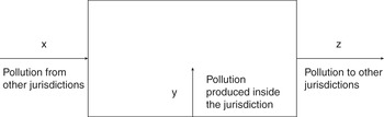
Figure C1 Box model that indicates the inflows and outflows in a given jurisdiction
We know from Table C1 that


where a approximates a constant. Therefore, y is equally proportional to w from year to year. While the wind spillover effects may influence the magnitude of the results, given the scaling a, they may not affect the statistical significance of the results.
Table C1 Percentages of provincial PM2.5 that came from within the province, 2010 and 2015 compared
| Province | 2010 | 2015 |
|---|---|---|
| Anhui | 58 | 56 |
| Fujian | 59 | 52 |
| Gansu | 67 | 66 |
| Guangdong | 65 | 63 |
| Guizhou | 63 | 62 |
| Hebei | 64 | 62 |
| Heilongjiang | 80 | 73 |
| Henan | 63 | 61 |
| Hubei | 58 | 56 |
| Hunan | 61 | 59 |
| Jiangsu | 50 | 59 |
| Jiangxi | 52 | 53 |
| Jilin | 52 | 61 |
| Liaoning | 67 | 67 |
| Shaanxi | 69 | 68 |
| Shandong | 59 | 63 |
| Shanxi | 69 | 67 |
| Sichuan | 72 | 66 |
| Zhejiang | 52 | 54 |
D Causal Mediation Analysis: Growth versus Regulation
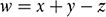
The causal mediation analysis approach circumvents the challenge of measuring pollution regulation.Footnote 39 Specifically, I perform a causal mediation analysis, where the treatment is a binary variable indicating whether an observation falls in the last year of a tenure and the outcome is average annual PM2.5 level. As shown in Figure D1, there are two pathways through which being in the last year in office can affect the average yearly PM2.5 level. Being in the last year can affect pollution indirectly via the economic growth pathway, where nighttime luminosity is a mediator. Being in the last year also has a direct effect via environmental regulation. Economic growth and environmental regulation are the two major human activities that influence pollution levels (Reference RingquistRingquist 1993). The direct and indirect effects of the treatment in prefecture i in year t is measured per Eqs. (D1) and (D2). The sign and magnitude of the average direct effect (ADE), the average causal mediation effects (ACME), and the total effect will help us understand the effects of these two mechanisms.
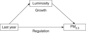
Figure D1 Causal mediation analysis of the effect of last year on the PM2.5 level
 (D1)
(D1)
 (D2)
(D2)
Table D1 presents the results for ADE, ACME, and the total effect from the causal mediation analysis, where the dummy variable, “last year,” is the treatment, and luminosity is the mediator.Footnote 40 ACME measures the effect of the luminosity-mediated pathway while ADE measures the residual effect, which in this context is mostly the effect of environmental regulation, on PM2.5.Footnote 41 As we can see, the ADE and the total effect bear positive signs while that for ACME is significantly negative, creating a situation of “inconsistent mediation.” Hence, the positive effect the treatment has on the outcome is entirely due to the direct mechanism of relaxing environmental regulation.
Table D1 Summary of results from the mediation analysis based on observations from 2000–10
| Treatment | Mediator | ADE (95% CI) | ACME (95% CI) | Total effect (95% CI) |
|---|---|---|---|---|
| Last year | Luminosity | 0.39 (-0.13, 0.90) | -0.12** (-0.18, -0.05) | 0.28 (-0.24, 0.79) |
Notes: Statistics are rounded to the second decimal place. 95% confidence intervals appear in parentheses under estimates of the average effects.
*p < 0.05
** p < 0.01
***p < 0.001
39 Precise measurements of regulatory stringency can be extremely challenging to create. The conventional practice is to use the pollution discharge levy rate as a proxy. However, actual pollution regulation stringency is nearly impossible to determine, and it may differ significantly from what is written on paper in a country like China. Hence, I pursue a causal mediation analysis for insights into this question.
40 Since the treatment has to be binary in causal mediation analysis, the setup here is different from the specification in the main equation.
41 The causal mediation approach assumes sequential ignorability (i.e., no additional channel that interacts with the specified mediator). Since this assumption is untestable but likely, a sensitivity analysis can provide information about how reliable the results are. However, in this particular setting, a sensitivity analysis cannot be implemented due to a computational singularity in the system, and this cannot be solved by removing certain variables. Future research focusing on a later period when more data becomes available can probe more deeply into the extent to which regulatory forbearance contributes to waves of pollution, using causal mediation or another appropriate method.

 Open access