


Impact Statement
The vertical-axis wind turbine or VAWT has yet to achieve commercial success primarily due to the complexity of the underlying fluid dynamics, which is much more intricate than that of the common horizontal-axis wind turbine. During each rotation, a blade on the VAWT rotor is subject to unsteady loading, even when the inflow is steady and uniform. Models of this turbine suffer from a lack of validation datasets at field-relevant conditions. Little is known regarding how the rotor aerodynamics are affected by geometrical changes, especially when moving from model-scale results to the field. In this work we tackle these challenges by investigating how the power performance of the VAWT depends on the geometrical rotor solidity and the physical size, or Reynolds number, at full-scale conditions. The achievement of full-dynamic similarity in controlled laboratory conditions make this a unique study. The data presented here can directly impact practical VAWT design by serving as a benchmark for computational design and modelling exercises, thereby increasing the reliability and safety of new VAWT turbines.
1. Introduction
Recently, there has been renewed interest in the aerodynamics of vertical-axis wind turbines (VAWTs), as they may have advantages over the more commonly used horizontal-axis wind turbines (HAWTs) when mounted on floating platforms offshore, as well as in niche markets not served by commercially available HAWTs (see e.g. Reference Bhutta, Hayat, Farooq, Ali, Jamil and HussainBhutta et al., 2012; Reference DabiriDabiri, 2011; Reference Griffith, Barone, Paquette, Owens, Bull, Simao-Ferriera, Goupee and FowlerGriffith et al., 2018; Reference Miller, Duvvuri, Brownstein, Lee, Dabiri and HultmarkMiller et al., 2018). One of the primary reasons that VAWT designs have remained less popular in the marketplace is the increased difficulty associated with modelling the performance of these units, which often results in overengineering or durability issues. Even when inflow conditions are steady, each blade experiences highly unsteady loads during every rotation cycle due to the large changes in the local angle of attack. This implies that many dynamic effects, which are not present during typical HAWT operation, affect the VAWT. Examples include dynamic stall of the airfoils, tower shadow, and flow curvature and expansion (Reference Borg, Shires and ColluBorg, Shires, & Collu, 2014; Reference Ferreira, Van Kuik, Van Bussel and ScaranoFerreira, Van Kuik, Van Bussel, & Scarano, 2009). In addition to considering these complex aerodynamics, many design decisions must be made regarding the geometrical features of the VAWT. A parameter which has historically been used to characterize the VAWT geometry in a single non-dimensional number is the solidity, which is the ratio of the open to closed area swept by the rotor:
 \begin{equation} \sigma_s = \frac{A_b}{A_s},\end{equation}
where  $A_b$ is the total blade planform area and $A_s$ is the rotor swept area. For a simple H-rotor design where the blades are of constant chord and located vertically, this definition reduces to a form which is independent of rotor height: $\sigma _s={N_b c}/{2 {\rm \pi}R}$, where $N_b$ is the number of blades, $c$ the blade chord length and $R$ the rotor radius. The power coefficient of the rotor, or percentage of free stream kinetic energy a turbine turns into useful power, is a critical metric for the commercial success of a wind turbine and has generally been found to increase as solidity is reduced. As can be seen for the H-rotor design, the solidity can be reduced in a number of ways such as a reduction in blade number or blade chord, or alternatively by an increase in the rotor radius. Although rotor solidity is an important parameter for characterizing VAWT performance, it does not encompass all geometrical features of a rotor such as airfoil selection, strut design, tower blockage or the ratio of lift to drag for each turbine blade. Some authors have attempted to aggregate these effects by using the ratio of chord to blade radius, $c/R$, which is essentially a measurement of the lift to drag ratio for each individual blade but has the benefit of being easy to calculate (Reference Fiedler and TullisFiedler & Tullis, 2009). In reality, all geometry changes will impact rotor performance to some extent and additional work is required to develop models which more accurately capture each of these changes.
Two additional parameters govern the performance of the VAWT: the tip speed ratio, which represents the rotational velocity of the rotor referenced to the free stream velocity, and the Reynolds number, which indicates the scale or ‘size’ of the machine, and are given by
 \begin{equation} \lambda = \frac{\omega R}{U} \quad Re = \frac{\rho U^ * L^ * }{\mu},\end{equation}
where  $\omega$ is the angular velocity, $U$ the free stream wind speed, and $\rho$ and $\mu$ the fluid density and viscosity, respectively. The velocity and length scale used for the Reynolds number, given by $U^*$ and $L^*$, can change depending on what specific details of the flow are of interest. A commonly used Reynolds number is defined using the local blade conditions, denoted as $Re_c$, which uses the blade chord length, $c$, and the velocity relative to the blade, $V_{rel}$. Another Reynolds number uses the rotor diameter and free stream velocity, denoted as $Re_D$. However, if the geometry and $\lambda$ values are matched between two studies then matching a single Reynolds number ensures that all other $Re$ are also matched, regardless of what specific $U^*$ and $L^*$ are chosen. Therefore, Reynolds numbers are typically chosen using some physical intuition or for convenience. Either way, the magnitude of the two most commonly used Reynolds numbers, $Re_c$ and $Re_D$, for the VAWT operating in the field are typically quite large, with values spanning $10^6$ to $10^8$. This creates a very challenging problem when scaled-down models are used for testing. To counteract the reduction in $L^*$ the velocity of the model must be increased. In this way $Re$ can be matched, but then it becomes impossible to match the model tip speed ratio to the full scale as velocity appears in the denominator of $\lambda$. As noted previously by Reference de Vriesde Vries (Reference de Vries1983) and Reference Adaramola and KrogstadAdaramola and Krogstad (Reference Adaramola and Krogstad2011), matching both the tip speed ratio and the Reynolds numbers of the full scale using small models in conventional wind tunnels is therefore not possible. As a consequence, only a few studies exist at Reynolds numbers which are comparable to the field scale and the full range of $Re$ from the model to field scale has not been extensively explored (no matter how $Re$ is defined). This has directly led to a lack of model validation data where all relevant geometrical ( $\sigma _s$) and flow ( $\lambda$, $Re$) conditions are matched with what a full-scale field turbine experiences. Given the aerodynamic complexity and large number of possible configurations for the VAWT, this lack of data has directly contributed to reduced confidence in modelling and design tools which remains a major hurdle for more widespread utilization of the VAWT.
Despite the lack of current datasets, there have been several significant past efforts to acquire full-scale or near-full-scale VAWT data, notably by Sandia National Labs with both field and large wind tunnel studies (Reference Blackwell, Sheldahl and FeltzBlackwell, Sheldahl, & Feltz, 1976; Reference WorstellWorstell, 1979). Early data taken with a 2 m diameter model in a wind tunnel showed that turbine performance improved with increasing Reynolds number for each given  $\lambda$ and all solidities tested, $\sigma _s \in [0.13,0.3]$ (Reference Blackwell, Sheldahl and FeltzBlackwell et al., 1976). A later field study used a slightly larger 5 m diameter model and showed a similar trend (Reference Sheldahl, Klimas and FeltzSheldahl, Klimas, & Feltz, 1980). Common to both of these studies is that the power coefficient continues to depend on the Reynolds number even at the highest tested values. Ideally, as $Re$ becomes increasingly large the flow should become insensitive to viscous effects, which implies that the power coefficient is constant despite continued increases in $Re$. This is sometimes referred to as Reynolds number-invariant or -independent behaviour, and can greatly simplify modelling by eliminating Reynolds number effects from consideration. However, it is very difficult if not impossible to predict when this will occur using only theory or simulations due to the complexity of the VAWT flow field. Continued sensitivity to Reynolds number indicates that larger models are necessary if conventional field or laboratory data are to be acquired. It was not until a much larger turbine with a diameter of 17 m was tested in the field that any invariant behaviour was directly observed (Reference WorstellWorstell, 1979). However, only a single solidity was tested ( $\sigma _s=0.14$) and the authors added a caveat that the highest tested $Re$ data point ( $Re_c \approx 1.45 \times 10^6$) may have contained an instrumentation error. Even with these limitations, it does indicate that a very large Reynolds number is potentially required for Reynolds number-independent behaviour. Numerical simulations have observed significant Reynolds number dependencies for a range of $\sigma _s = 0.041$ up to $0.251$ (Reference Lohry and MartinelliLohry & Martinelli, 2016). Near-invariant behaviour was observed at the largest Reynolds numbers simulated which exceeded $Re_c > 30 \times 10^6$, and corresponded to rotor diameters of $D \approx 50$ m. Recent work by the authors compared field and laboratory measurements of a single VAWT with a solidity of $\sigma _s=0.36$ (Reference Miller, Duvvuri, Brownstein, Lee, Dabiri and HultmarkMiller et al., 2018). Reynolds number invariance in the power coefficient was not seen in the field data, but was observed in the experiments, which achieved twice the $Re$ of the field (regardless of how $Re$ is defined). Large values of the blade Reynolds number were required in the lab for this behaviour to occur ( $Re_c \geq 1.5 \times 10^6$, based on the blade chord and local velocity), which was surprisingly close to the values reported by Reference WorstellWorstell (Reference Worstell1979) for a VAWT operating in the much more variable conditions in the field and with a very different configuration and solidity value. All of this is to say that potentially very large Reynolds numbers are required for complete invariance to $Re$; however, these examples have shown that invariant behaviour is possible in field, numerical and experimental work.
The present work more fully explores the operational space of the high-solidity VAWT for a range of  $\sigma _s$ values by matching $\lambda$ and $Re$ simultaneously to field-relevant conditions. To accomplish this, a specialized wind tunnel was used which operates with highly compressed air as the working fluid (as described in the earlier work of Reference Miller, Duvvuri, Brownstein, Lee, Dabiri and HultmarkMiller et al., 2018; Reference Miller, Kiefer, Westergaard, Hansen and HultmarkMiller, Kiefer, Westergaard, Hansen & Hultmark, 2019). The high static pressure inside the tunnel decreases the fluid kinematic viscosity by up to two orders of magnitude over air at atmospheric pressure. This allows for high Reynolds numbers using relatively small models and low free stream velocities. The model geometry was based on a commercially produced, field-scale wind turbine and was previously compared to field measurements at a single solidity (Reference Miller, Duvvuri, Brownstein, Lee, Dabiri and HultmarkMiller et al., 2018). Modifications were made to the VAWT model so that the blade number and therefore turbine solidity could be easily altered. The resulting dataset spanned a large operational space of $\sigma$, $Re$ and $\lambda$ values for the VAWT. By increasing the parameter space of the experiments, we aim to examine the applicability of earlier scaling results found for the 5-bladed turbine regarding Reynolds number behaviour. As discussed in the following, Reynolds number effects can be straightforwardly captured by a single $Re$ parameter for a larger range of solidity values than previously established. However, some deviations are seen from the trends as $Re$ increases and $\sigma$ decreases which may point to a change in the underlying aerodynamic behaviour at low-solidity values.
2. Experimental Facility
To achieve field-scale Reynolds numbers on the vertical-axis wind turbine model, a specialized, high-static-pressure wind tunnel known as the High Reynolds number Test Facility (or HRTF) was utilized. The wind tunnel is a closed-loop, recirculating type designed to operate at very high static pressures, but relatively low velocities using compressed, dry air as the working fluid. The HRTF can support static pressures up to 233 bar and free stream velocities up to 10 m s $^{-1}$.
For a facility operating with compressed air as the working fluid, density is given by the real-gas relationship
 \begin{equation} \rho = \frac{ p_{s}}{ZRT},\end{equation}
where  $R$ is the specific gas constant for air, $T$ the tunnel temperature, $p_{s}$ the static pressure and $Z$ the compressibility factor. For dry air, $Z$ changes by only $10\,\%$ for values of $p_{{s}}$ over the range 0–233 bar, which means that for a constant temperature, density is nearly linearly related to pressure. This implies that a model operating near the maximum $p_{s}$ of the HRTF will see mechanical loads which are in excess of 200 times that seen by the same model operated at the same flow speed and atmospheric pressure, as evident from (3.1). For this reason, considerable care has been given to the mechanical design of models, measurement equipment and support structures. The key to achieving dynamic similarity in this facility is not only the high static pressure, but also that dynamic viscosity and sound speed are only weak functions of $p_{s}$. The value of $\mu$ changes by $30\,\%$ and $a$ by $12\,\%$ from their values at atmospheric to full tunnel pressure, in contrast with density which increases $21\,900\,\%$ (all determined using real-gas relationships). For all experimental results, the exact density and viscosity of the compressed air are found using real-gas relationships with measurements of $p_{s}$ and $T$, as outlined by Reference ZagarolaZagarola (Reference Zagarola1996).
A schematic of the HRTF is shown in Figure 1. The tunnel contains two test sections with a total length of 4.88 m; each having a circular cross-section with an inner diameter of 0.49 m. The test sections are preceded by a contraction with an area ratio of 2.2 : 1, in which are located a series of honeycomb flow straighteners and conditioning screens. These devices are configured to produce a laminar, slug-type flow inside the test sections with a measured turbulence level of  $0.3\,\%$ at the lowest tunnel Reynolds number and $1.1\,\%$ at the highest (Reference Jiménez, Hultmark and SmitsJiménez, Hultmark, & Smits, 2010). Thus operation of the facility is very similar to a conventional, atmospheric wind tunnel designed for laminar test-section flow. The HRTF is not actively cooled, and does experience temperature increases in the working fluid if the runtime is sufficiently long, especially at high tunnel pressures and velocities. For these experiments, the runtimes were kept short and tunnel heating was minimized. In addition, any small temperature and static pressure changes during a run were measured and used to determine the true fluid properties using real-gas relationships. This facility, and the data processing and reduction techniques have been detailed in prior work using this facility (Reference Miller, Kiefer, Westergaard, Hansen and HultmarkMiller et al., 2019).

Figure 1. Schematic diagram of the HRTF as viewed from above the facility. The figure labels correspond to: the 150 kW pump motor (a), the flow conditioning and contraction (b), and the two test sections (c).
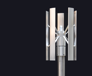
Models were installed in the HRTF via a single 0.254 m access port located on the top of the facility. Wind turbine models were controlled via the measurement stack which was mounted inside this access port. A measurement stack was designed to interface with the vertical-axis wind turbine model and accurately resolved the forces and moments produced by the model and controlled the turbine rotational speed. The entire assembly was located inside the pressurized environment of the HRTF with only electrical feedthroughs to the atmospheric side. The fundamental components of the measurement stack were a load cell for measuring forces and moments, a torque transducer for shaft torque and rotational speed measurement, and a brake for speed control. All of these components were located on an aluminium carriage structure which allowed the entire measurement stack to be removed at once from the facility. The measurement stack, as mounted in the HRTF with the VAWT model, is shown in Figure 2.

Figure 2. Rendering of VAWT model in a cutaway of the HRTF test section. Labels correspond to (a) 5-bladed VAWT model, (b) tower housing, (c) six-component force/moment sensor, (d) torque transducer with speed encoder and (e) magnetic hysteresis brake for speed control. Flow direction is given by the red arrow.
2.1 Vertical-axis Wind Turbine Model
The VAWT model was initially based on a commercially available design with a scale reduction of 1 : 22.5, as discussed in an earlier work (Reference Miller, Duvvuri, Brownstein, Lee, Dabiri and HultmarkMiller et al., 2018). Details of the model used in this study are given in Table 1 with the main geometric features of the full scale retained on the model. Small changes were made to the model hub and support tower to accommodate the increased mechanical loads present, as detailed by Reference Miller, Duvvuri, Brownstein, Lee, Dabiri and HultmarkMiller et al. (Reference Miller, Duvvuri, Brownstein, Lee, Dabiri and Hultmark2018).
Table 1. Vertical-axis wind turbine model geometry fixed for all solidity cases.

The scale reduction chosen for the model allowed for a relatively small blockage ratio of  $8.36\,\%$. In addition, thrust coefficient values for this turbine often exceeded unity during the tests and so no blockage corrections were applied to the resulting datasets. Additional simulations or experimental work with a variety of models would be required to determine a suitable blockage correction at high-thrust levels for these cases due to failure of the quasi-one-dimensional assumptions used when deriving the classical porous plate blockage correction based on the work of Reference GlauertGlauert (Reference Glauert1935), but discussed in many other works (see e.g. Reference Bahaj, Molland, Chaplin and BattenBahaj, Molland, Chaplin, & Batten, 2007; Reference Chen and LiouChen & Liou, 2011; Reference MikkelsenMikkelsen, 2004; Reference Ross and PolagyeRoss & Polagye, 2020). However, in all tests the low-geometric blockage of the turbine was kept constant to minimize any resulting blockage effects.
Manufacturing of the model was performed using computer numerical controlled machining processes and the blades were formed from solid blocks of 7075 aluminium alloy. The area-averaged root-mean-square roughness height of the model airfoil was measured with a confocal microscope (Olympus LEXT OLS4000) and was found to be  $S_q = 0.5 \pm 0.25\ \mathrm {\mu }$m.
In an effort to expand the experimental scope beyond the fixed 5-blade rotor case, several interchangeable hubs were produced such that the number of blades could be reduced to 4, 3 or 2. This allowed for quick variation of the turbine solidity by alteration of the blade number. Changing only the blade number has several key advantages when investigating solidity effects such as keeping the  $c/R$ ratio and geometrical blockage effects constant for all configurations. The resulting dataset was therefore representative of pure rotor solidity changes where $c/R$, lift to drag ratio or other geometric changes are not varied between cases. The 5-blade data have been presented along with field measurements in a prior work (Reference Miller, Duvvuri, Brownstein, Lee, Dabiri and HultmarkMiller et al., 2018) while the 4-, 3- and 2-bladed data are new. The different configurations along with the solidity values are shown in Figure 3.

Figure 3. Various hub configurations for the VAWT which allow for altering the solidity by using 2, 3, 4 or 5 blades. Figure reproduced from Reference Duvvuri, Miller and HultmarkDuvvuri, Miller, and Hultmark (Reference Duvvuri, Miller and Hultmark2018).
3. Results
For wind turbines operating in the field, performance data are typically given as a function of the tip speed ratio only. When viewing data in this manner, only the incoming wind velocity is changing along the abscissa, which decreases with increasing  $\lambda$ because the rotation rate is effectively fixed (for machines that use asynchronous generators such as the FloWind 19 m, described by Reference BergBerg, 1996). By definition, this means that the Reynolds number, $Re_D$, is increasing along the abscissa. Hence, it makes little sense to plot the data as a function of $Re_D$ separately. For these experiments, a completely different control method was used for the model. Full authority over rotation rate was provided by the use of a magnetic hysteresis brake meaning that any rotation speed from free-wheeling (no-load) to complete locking of the rotor could be prescribed. In addition, the density and inflow velocity could be set independently of the turbine rotation rate. In this way, the data of the current experiment were different than the field data because the free stream conditions remained constant (i.e. $Re_D$ remained constant) and only the turbine rotational rate (and consequently the tip speed ratio) varied along the abscissa of the plots in Figure 4. Each colour-coded line represented a different $Re_D$ value: after adjusting the inflow characteristics to yield a certain Reynolds number, $Re_D$, the turbine was allowed to freely rotate and then small braking load increments were prescribed up until just before the turbine stalled (these loads were determined empirically beforehand). In this way, the plots of this paper were different than field data as the Reynolds number, $Re_D$, and the tip speed ratio, $\lambda$, were completely decoupled. Results are presented in the following as a function of the non-dimensional rotor power coefficient:
 \begin{equation} C_P = \frac{\omega \tau}{1/2 \rho U_\infty^3 {\rm \pi}R^2},\end{equation}
where  $\tau$ is the shaft torque and $U_\infty$ the free stream velocity.

Figure 4. Power coefficient as a function of tip speed ratio for four different VAWT rotor solidities. Colour gives the mean  $Re_D$ value for each power curve. Two additional, high-Reynolds-number runs are available for the $\sigma _s=0.21$ rotor at $Re_D=5.93 \times 10^6$ for the grey-filled square symbols and at $Re_D = 7.19 \times 10^6$ for the red-filled diamond symbols. Solid lines are cubic polynomial fits to the data.
Data sets for the four solidities,  $\sigma _s= 0.14$, $0.21$, $0.29$ and $0.36$ (corresponding to $N_b = 2$, $3$,
$3$,  $4$ and $5$ blades, respectively) are compared as a function of the free stream Reynolds number, $Re_D$, in Figure 4. The $\sigma _s=0.36$ case is shown here repeated from the earlier work of the authors for comparison purposes (Reference Miller, Duvvuri, Brownstein, Lee, Dabiri and HultmarkMiller et al., 2018). Significantly more data were acquired for the highest solidity 5-bladed rotor because it was the subject of a direct comparison with the commercial field unit on which it is based. We also note that this turbine configuration was significantly easier to run experimentally, exhibiting earlier startup at lower wind speeds and more gentle stall behaviour at low tip speeds. This second behaviour led to a larger operating space to the left of the peak in $C_P$ (i.e. tip speed ratios lower than ideal) when compared with the lower solidity configurations. Note that the model used in this study was only powered by the flow, so it could not be artificially forced to operate at a specific tip speed ratio. The highest and lowest $\lambda$ for each configuration could then be considered as the actual limits of operation for a full-scale turbine of this geometry. This configuration was also the most amenable to operation at lower Reynolds numbers. During experimental runs, we attempted to gather data on the other configurations at the same Reynolds numbers as the $\sigma _s=0.36$ case, but were not always able to keep the model running in these conditions. This was likely related to the averaging effect on shaft torque caused by having a higher blade number. If an individual blade moved into stall, the higher total blade count made it more difficult to overcome the larger rotor inertia and summed torque contributions of the other blades. This is another benefit of high-solidity turbine designs.
The  $\sigma _s=0.36$ case showed a maximum power coefficient at a tip speed of $\lambda =1$ and the location of this peak did not appear to depend on the specific $Re_D$ value chosen. The low operating tip speed ratio was consistent with the high solidity of the turbine geometry. When the solidity was reduced to $\sigma _s=0.29$, a higher maximum power coefficient was possible with an accompanying slight shift to $\lambda = 1.1$. The trend continued for the $\sigma _s=0.21$ case, with max $C_P$ typically occurring near $\lambda = 1.3$. Note that two additional high- $Re_D$ datasets were available for the $\sigma _s=0.21$ turbine, one at $5.93\times 10^6$ and another at $7.19 \times 10^6$. Datasets were very difficult to acquire at these Reynolds numbers as these required running the HRTF at maximum static pressure and near maximum velocities. For the highest $Re_D$ case, the peak in $C_P$ was not captured; however, a small clustering of data points was seen around $\lambda =1.35$. This case unfortunately corresponded to a natural frequency observed in the $N_b=3$ bladed rotor configuration, and caused large torque fluctuations about the mean increasing the uncertainty of these points.
Interestingly, the performance improvement near maximum  $C_P$ caused by reducing solidity from $\sigma _s=0.36$ to $0.29$ was not large at $6.9\,\%$, and was only $4.8\,\%$ when further reducing the solidity from $0.29$ to $0.21$ (ignoring the highest tested $Re_D$ case). Despite the overall low performance of this turbine in any configuration, the $N_b=5$ blade turbine does operate in the same performance envelope as the full scale on which it is based (Reference Miller, Duvvuri, Brownstein, Lee, Dabiri and HultmarkMiller et al., 2018). In the interest of making a direct determination of solidity effects, we only elected to reduce the number of blades on the model to reduce solidity, all other geometric details were kept intact. It is likely that this turbine geometry is far from ideal and a high solidity design does not translate well to lower solidity values as effects such as tip losses become increasingly important at higher $\lambda$. For the lowest solidity case, $\sigma _s=0.14$, maximum performance behaviour was not immediately clear, but $C_P$ may have decreased slightly with $Re_D$. The reason for this result may be related to the large fluctuating loads exhibited by the 2-bladed turbine. The standard deviation of shaft torque from the mean was always between 55 % and 90 % of the mean for the lowest solidity rotor, values which only occurred on the other configurations when operating near rotor natural frequencies (which was avoided if possible). With less blades to smooth out the cyclic variation in torque, we would expect the fluctuations in mechanical loading to become higher, especially if operational tip speeds are low. However, the 2-bladed behaviour could also indicate a change in the underlying rotor aerodynamics at low solidity and high $Re$. Future work will specifically examine the low-solidity rotor behaviour, with the present work maintaining focus on the three highest solidity cases where clear Reynolds number trends were observed in $C_P$.
All three highest solidity cases exhibited similar Reynolds number trends, with performance generally improving as  $Re_D$ was increased. A plateau behaviour was also observed near the peak in $C_P$ of Figure 4. Above a certain Reynolds number, performance ceased to depend on additional increases in $Re_D$, a clear indicator of power coefficient invariance to Reynolds number. Close observation of the plots in Figure 4 also indicated that the specific $Re_D$ at which the rotor performance became invariant also depended on $\lambda$, with higher tip speed ratios showing $C_P$ invariance at lower $Re_D$ values. A two-parameter dependence indicated that a single non-dimensional group may better capture the behaviour of $C_P$. Similar to prior work on the 5-bladed rotor, we utilized a chord-based Reynolds number in an attempt to capture this trend:
 \begin{equation} Re_c = \frac{\rho c (U + \omega R)}{\mu} = Re_D \frac{c}{D} (1 + \lambda).\end{equation}
 When computed, the value of  $Re_c$ given by (3.2) is the nominal maximum blade Reynolds number in the absence of rotor induction for a certain geometry, rotation rate and inflow condition. This definition has the benefit of also being convenient to calculate since measurements of the actual relative velocity at the blade are not possible with the current set-up. The datasets of Figure 4 can then be recast in terms of blade $Re_c$. To perform an analysis of this type, the data were first interpolated to a fixed $\lambda$ grid so that we could also directly analyse the effects of rotation. The interpolation operation introduced only a small amount of error, as the power curves for each rotor were highly resolved, containing twelve or more individually measured data points. Following this step, bin averaging was performed on the values at each tip speed by Reynolds number. As discussed in § 3.1, for most of the low-Reynolds-number cases the unique nature of the HRTF allowed for capturing the same $Re_D$ multiple times with different velocity and density combinations. It was not always possible to exactly match $Re$ between datasets due to small shifts during tunnel operation, but the bin-averaging error was relatively small because $Re_D$ was matched within $\pm 4.6 \times 10^4$ or less with different physical combinations of $\rho$ and $U$. Experiments in traditional wind tunnels cannot validate data in this manner and this gives additional confidence in the reported dataset. The resulting $C_P$ versus $Re_c$ curves are shown for the four different solidities in Figure 5.

Figure 5. Power coefficient for the VAWT model at various solidities as a function of blade Reynolds number. Symbols indicate the tip speed ratio, legend applies to all plots.
A number of observations can be made from these plots. First, it was straightforward to determine the optimal  $\lambda$ across the entire Reynolds number range. As noted in the earlier plots of $\lambda$ and $Re_D$, the peak in performance for the $\sigma _s=0.36$ turbine was $\lambda = 1$ for all Reynolds numbers, although there was some overlap at lower values of $Re_c$. The next highest solidity case peaked at a slightly higher tip speed ratio of $\lambda = 1.1$. The $\sigma _s=0.21$ rotor showed an even higher optimal tip speed of $\lambda = 1.3$. The two additional high- $Re_D$ power curves acquired for the $\sigma _s=0.21$ case also resulted in a much wider range of $Re_c$. Results were less clear for the lowest $\sigma _s=0.14$ case, a tip speed of between 1.4 and 1.5 seemed to yield the maximum $C_P$.
As  $Re_c$ increased, the $\sigma _s=0.29$ rotor power coefficient eventually became invariant to additional increases in the Reynolds number. Here the cutoff value for $Re$ invariance interestingly occurred at approximately the same value of $Re_c = 1.5 \times 10^6$ as prior work reported for the higher solidity rotor (Reference Miller, Duvvuri, Brownstein, Lee, Dabiri and HultmarkMiller et al., 2018). The $\sigma _s=0.21$ rotor showed a similar trend with invariance appearing to occur above the same threshold $Re$ value. However, for the very high $Re_c$ datasets, there was a small decrease in $C_P$ as $Re$ continued to increase. For instance, the $\lambda =1.4, 1.5$ and $1.6$ cases indicated a slight decrease and then increase in $C_p|_\lambda$ when $Re_c > 2.5 \times 10^6$. This was a reflection of the data points mentioned earlier in Figure 4 which were taken near the rotors natural frequency out of necessity of the run conditions. Results from the lowest solidity rotor were less clear, with an increased dependence on $Re_c$ observed at increased Reynolds numbers. At first it was suspected that the highly fluctuating loads of this rotor were causing errors in determining the mean quantities. However, as discussed in the following section, these datasets have been extensively validated in the wind tunnel. Another possibility was that the aerodynamics governing the lower solidity turbine scale quite differently than the high-solidity, $\sigma _s=0.36$ to $0.21$ cases. In this case, different rotor aerodynamics may be at work for high- $Re$, low-solidity VAWTs.
3.1 Data Validation for Low-solidity Rotors at Large Reynolds Numbers
To validate the results of the low-solidity turbine, we employed a method similar to that previously used for the  $\sigma _s=0.36$ rotor by Reference Miller, Duvvuri, Brownstein, Lee, Dabiri and HultmarkMiller et al. (Reference Miller, Duvvuri, Brownstein, Lee, Dabiri and Hultmark2018). The HRTF allows for altering the tunnel pressure and free stream velocity independently to achieve the same Reynolds number. Using dynamic similarity in this way allows for different mechanical loads to be placed on the rotor and measurement stack, which should collapse when non-dimensionalized as the power and thrust coefficients versus tip speed ratio. For the lower Reynolds numbers of all four turbine configurations, many validation datasets are available due to the relative ease of achieving $Re_D < 4 \times 10^6$ with different static pressure and velocity combinations in the wind tunnel. However, the highest $Re$ cases are challenging to run because the tunnel must be set to the maximum static pressure and the largest velocity that the model can mechanically sustain. This means that the highest Reynolds number cases typically cannot be validated in the same way as the lower $Re$ ones. However, several validation datasets were acquired at a relatively large $Re \approx 4 \times 10^6$ condition for all turbine configurations in an effort to confirm the observed trends. A representative dataset is shown in Figure 6 for the lowest solidity rotor at a matched Reynolds number of $Re_D=3.938 \times 10^6 \pm 4.1 \times 10^3$. The small variation in $Re$ existed due to the difficulty of exactly matching the flow velocity to the desired value. The plot also shows the measurement uncertainty associated with the dimensional and non-dimensional plots. For the dimensional case, the uncertainty was seen to be very small relative to the mean value, but the non-dimensional plots showed a much larger uncertainty due to the velocity cubed term in the power coefficient. There were some small deviations between datasets at high- $\lambda$ values due to the small-torque values measured. However, despite being one of the more difficult cases to validate, we still observed good collapse especially near the peak in performance. For this reason we have a high level of confidence in the reported trends for the low-solidity, high- $Re$ datasets of Figure 5 but comment that we were unable to validate the highest Reynolds number ( $Re_D > 4 \times 10^6$, for all $\lambda$) cases due to facility limitations. The general trend in $C_P$ for datasets near $Re \approx 4 \times 10^6$ was maintained even at higher $Re$, so it was therefore unlikely that experimental uncertainty was the reason for the observed behaviour. Using this validation method, the performance trends observed for all solidity configurations when $Re_D \leq 4 \times 10^6$ were accurate.

Figure 6. Dimensional power and rotation rate for the 2-blade turbine are shown for various tunnel conditions in panel (a) at a fixed Reynolds number of  $Re_D=3.938\times 10^6 \pm 4.1 \times 10^3$. The data are then non-dimensionalized and plotted in panel (b) to illustrate data collapse due to dynamic similarity. The grey bars indicate measurement uncertainty of the data. The legend applies to both plots.
3.2 Reynolds Number Trends
Comparing the Reynolds number trends with previous high- $Re$ work, the field data of Reference WorstellWorstell (Reference Worstell1979) reported the power coefficient as a function of blade Reynolds number, although a slightly different definition of $Re_c$ was used. When converted to the definition of $Re_c$ in this work, invariant behaviour in $C_{P,{max}}$ was indicated when $Re_c \geq 1.45 \times 10^6$ (Reference WorstellWorstell, 1979 noted that the data points used for this trend may contain errors due to measurement uncertainty, as discussed earlier in this text. This in part motivated the current study to collect additional, high- $Re$ datasets). This was a surprising result as the turbine geometry differed significantly from the simple H-rotor Darrieus configuration presented here; however, the solidity matched our lowest case at $\sigma _s = 0.14$. It should be noted that both studies used an airfoil from the same NACA family, in the case of the study by Reference WorstellWorstell (Reference Worstell1979) a 0012 airfoil was used, whereas the present work utilized a 0021 airfoil. It is likely that the specific value of the cutoff Reynolds number depends on the airfoil family used for the blades. The cutoff $Re_c$ furthermore coincided with the lower end of the design Reynolds number for this NACA series (Reference Abbott and Von DoenhoffAbbott & Von Doenhoff, 1959; Reference SchmitzSchmitz, 2019). These series were originally intended for use on aircraft operating at much larger $Re$ than small to medium scale wind turbines which further emphasized that airfoil selection must be carefully considered when performing experiments at reduced scale.
The plots of Figure 5 indicated that the  $\sigma _s=0.29$ and $\sigma _s=0.21$ data required a Reynolds number of $Re_c \geq 1.5 \times 10^6$ for $Re$ invariance in $C_P$, similar to prior tests with a $\sigma _s=0.36$ rotor. Reynolds number invariant behaviour is important as it sets a threshold value to achieve in simulations and experiments, under which the flow physics will be different. For the $\sigma _s=0.29$ data, the highest Reynolds number data were available at $Re_c = 3.119 \times 10^6$ while for the $\sigma _s=0.36$ rotor, $Re_c = 2.354 \times 10^6$ was the largest test value, which meant this data sufficiently covered and extended to very large-scale field rotors. The $\sigma _s=0.21$ data had the highest tested $Re_c \approx 4.75 \times 10^6$, but with the caveat that the two highest tested $Re_D$ cases from which this data were derived could not be validated directly with our method (as discussed in § 3.1), and excessive vibration was observed due to operating near the rotor natural frequency. To evaluate the utility of a $Re_c$ threshold, we normalized the data in two steps; the Reynolds invariant performance curve, denoted $C_{P,\infty }$, was first determined by averaging the values of $C_P|_\lambda$ in Figure 5 above our cutoff $Re_c$ of $1.5 \times 10^6$ for each individual tip speed ratio (to reduce experimental uncertainty). The $C_{P,\infty }$ values were thus functions only of $\lambda$ and $\sigma$. These plots are shown in Figure 7 and were similar in function to those shown in Figure 4, except they showed only the curve at the high-Reynolds-number limit. In addition, these curves were fit with a polynomial surface as given by (3.3). The fit was evaluated for the acquired range of $\lambda$ and $\sigma _s$ values and shown in Figure 7 as solid lines.
 \begin{align} C_{P,\infty} & = {-}3.762 + 5.367 \lambda + 13.96\sigma -2.2\lambda^2 -12.2 \lambda\sigma \nonumber\\ &\quad -14.45 \sigma^2 + 0.299 \lambda^3 + 1.92 \lambda^2\sigma + 8.483\lambda \sigma^2. \end{align}
Figure 7. Reynolds invariant power coefficient as a function of tip speed ratio for varying solidity. Colour indicates solidity/blade number:  $\sigma _s = 0.36$ are black; $\sigma _s = 0.29$ are green; $\sigma _s = 0.21$ are red.
It was apparent that solidity does play an important role in the global turbine performance. Namely, for high-solidity values it determines the shape of the Reynolds invariant power curve. What is not clear is how the lower  $Re_c$ behaviour is affected by solidity. It was demonstrated by Reference Miller, Duvvuri, Brownstein, Lee, Dabiri and HultmarkMiller et al. (Reference Miller, Duvvuri, Brownstein, Lee, Dabiri and Hultmark2018) that $C_P$ for the $\sigma _s=0.36$ rotor had a similar dependence on $Re_c$ regardless of the tip speed ratio. To evaluate whether this observation holds for lower solidities, and likewise how solidity affects the $Re_c$ behaviour, the data of Figure 5 were then combined with those of Figure 7. For each solidity and tip speed ratio, the power coefficients of $C_P|_\lambda$ were reduced by their respective $C_{P,\infty }$ value. In this way, above the cutoff $Re_c$, the parameter approached unity. This effectively removed the rotational and solidity effects allowing for direct evaluation of Reynolds number for the three highest solidity rotors.
In general, excellent collapse is seen in Figure 8 for the  $\sigma _s=0.36$, $0.29$ and $0.21$ rotor data to a single curve. Also shown is the curve fit of Reference Miller, Duvvuri, Brownstein, Lee, Dabiri and HultmarkMiller et al. (Reference Miller, Duvvuri, Brownstein, Lee, Dabiri and Hultmark2018) as a solid grey line, generated using only the highest solidity rotor and replicated here in (3.4). It appears this fit effectively captured the $Re$ dependence of the other two highest solidity cases as well, although less low- $Re_c$ data were available for the two lower solidity rotors because they tended to operate at higher $\lambda$ values. For the $\sigma _s=0.21$ rotor, there was a slight decrease for $Re_c > 3 \times 10^6$, likely due to system harmonics as previously discussed, with the largest deviating point still falling within $5.5\,\%$ of the invariant $C_{P,\infty }$ value:
 \begin{equation} \left. \frac{C_P}{C_{P,\infty}} \right|_\lambda = 0.3 \textrm{erf} \left( \frac{1.627 Re_c}{10^6} - 0.6443 \right) + 0.7.\end{equation}
Figure 8. Power coefficient normalized by the Reynolds invariant value for three different VAWT rotor solidities. Symbol indicates  $\lambda$, as in figures 5 and 7. Colour indicates solidity: $\sigma = 0.36$ are black; $\sigma = 0.29$ are green; $\sigma = 0.21$ are red. The grey line is the curve fit from (3.4).
The high level of collapse of the data in Figure 8 indicated that the power loss at small scale was only a function of the Reynolds number and not the tip speed ratio or the solidity. The effect of changing  $\lambda$ and $\sigma$ was relegated to determination of the $C_{P,\infty }$ curve for the three highest solidity cases. We therefore postulate that a decoupling of parameters occurs for the VAWT:
 \begin{equation} C_P = f(Re_c)g(\lambda, \sigma) \end{equation}
for the range of Reynolds numbers and three highest solidity values tested. The empirically determined functional dependencies were used for the Reynolds number term  $f(Re_c) = {C_P}/{C_{P,\infty }}|_\lambda$ and $g(\lambda ,\sigma ) = C_{P,\infty }$ for the dynamic effects, where $f$ is given by (3.4) and $g$ can be found using the functional relationship given by (3.3) and shown in Figure 7. Variations in $\sigma$ and $\lambda$ drove unsteady effects such as dynamic stall, Coriolis and centrifugal forces as well as wake–blade interactions (see for example Reference Rezaeiha, Montazeri and BlockenRezaeiha, Montazeri, & Blocken, 2018; Reference Tsai and ColoniusTsai & Colonius, 2016). Given this, a variation in the Reynolds number appeared to only affect the quasisteady physics of the VAWT, such as airfoil boundary layer development, while leaving the dynamic phenomena unaltered. Recent simulations using a NACA 0012 airfoil operating in dynamic stall indicated a reduced sensitivity to Reynolds number effects when the chord $Re$ is above 1 million (Reference Benton and VisbalBenton & Visbal, 2019). However, this has not been extensively confirmed at the high Reynolds numbers present in this study. It was also not apparent which of the dynamic effects are of primary importance to the high-solidity VAWT operation. However, Figure 8 indicated that whatever dynamic phenomena were present, they scaled independently of the Reynolds number.
4. Conclusions
Utilizing a compressed air wind tunnel facility, the experiments performed here explored a new operational space of the VAWT in detail for a range of rotor solidities and Reynolds numbers, up to and exceeding those of the field turbine upon which the initial model was based. The results demonstrated that Reynolds number invariance for VAWTs is possible in a laboratory setting using small-scale models of field relevant geometries (including airfoil profiles and aspect ratios). The unique capabilities of the HRTF were leveraged to acquire a large dataset including more than a decade of  $Re_D$, for four different values of solidity, $\sigma$. A chord-based Reynolds number was found to most appropriately capture Reynolds number trends in the power coefficient for the three highest solidity cases, $\sigma _s = 0.36$ ( $N_b = 5$), $\sigma _s = 0.29$ ( $N_b = 4$) and $\sigma _s = 0.21$ ( $N_b = 3$). The lowest solidity case, $\sigma _s = 0.14$ ( $N_b=2$), did not show a clear Reynolds number trend. This result was confirmed by extensive data validation and points to a possible change in the underlying aerodynamic scaling of lower-solidity VAWTs at high Reynolds numbers. Future work will explore this operational space in detail. For the three highest solidity rotors, a threshold $Re_c \gtrapprox 1.5 \times 10^6$ was determined by inspection to characterize the point at which $C_P$ ceased to depend on the blade Reynolds number for these three solidity cases. Simulations and field experiments from prior works also exhibited similar cutoff $Re$ values. We postulate that although the referenced works varied in the exact turbine geometry used, all rotors employed a NACA airfoil from the same family as this work. From this we suspect that the cutoff $Re_c$ value is likely related to the choice of airfoil family, although future work is needed to investigate this in detail.
With the observed Reynolds invariance, a power curve which was insensitive to additional increases in the Reynolds number (denoted  $C_{P,\infty }$) was found by averaging $C_P|_\lambda$ above the threshold $Re_c$ value. The $C_P|_\lambda$ data at all Reynolds numbers were then normalized by their respective $C_{P,\infty }|_\lambda$ values to directly evaluate $Re$ dependence below the observed threshold. All three high-solidity cases showed a similar Reynolds number trend below $Re_c = 1.5 \times 10^6$, which indicated that for high-solidity VAWTs the mechanisms resulting in power loss due to low Reynolds number are independent of both tip speed ratio and solidity. In contrast, the ultimate, high-Reynolds-number performance (i.e. the specific value of $C_{P,\infty }|_\lambda$) of the turbine is clearly governed by the solidity and tip speed ratio. Therefore the role of $\lambda$ at low Reynolds numbers is only to alter the relative wind speed at the rotor blade, and thus $Re_c$. This finding has important implications for the modelling and simulation of VAWT rotor aerodynamics. Despite the apparent complexity of the flow field due to unsteady blade loading during a single rotational cycle, we can effectively separate the Reynolds number and geometrical effects (i.e. $\sigma$ and $\lambda$) for all tested Reynolds numbers. This drastically reduces the amount of testing needed to determine aerodynamic performance. In addition, it points to a minimum Reynolds number at which the turbine should be operating so as to achieve optimal $C_P$. In the field this would be analogous to changing the physical size of the turbine for a given wind speed so as to avoid Reynolds number effects.
Funding Statement
The support of the National Science Foundation under grant CBET-1652583 is gratefully acknowledged.
Declaration of Interests
The authors report no conflict of interest.
Data Availability Statement
The data that support the findings of this study are openly available by contacting the authors directly via email.


 Open access