


1. Introduction
The origins of the fields of vortex dynamics and topology are intricately intertwined (Moffatt Reference Moffatt2008). Von Helmholtz (Reference von Helmholtz1858) developed equations describing vorticity field evolution in idealized fluid flow and proposed the notion of vortex lines. His seminal work in German was translated into English with some enhancements by Tait (Reference Tait1867). The concept of vortex lines served as inspiration to Kelvin (Reference Kelvin1867, Reference Kelvin1869) who hypothesized the ‘vortex theory of atoms’. According to this theory, matter is constituted of interconnected and knotted vortex filaments. The theory of atoms motivated a series of papers by Tait (Reference Tait1877, Reference Tait1884, Reference Tait1885) to characterize and classify knotted filaments. Although the vortex theory of atoms has long been disavowed, Tait's investigation of knots served as the foundation for the discipline of topology (Epple Reference Epple1998). Moffatt (Reference Moffatt1969) conducted extensive investigations of knottedness of vortex lines and developed the relation between knot topology and energy spectrum (Moffatt Reference Moffatt1990). In more recent times, Scheeler et al. (Reference Scheeler, van Rees, Kedia, Kleckner and Irvine2017) provided a complete measurement of helicity (linkage of vortex lines) in real fluid flows by tracking the linking, twisting and writhing of vortex lines. The measurements indicated that helicity can remain conserved or evolve towards a constant even in the presence of viscosity.
Vortex dynamics plays a crucial role in many fluid flow phenomena (Saffman Reference Saffman1992). Indeed, Küchemann (Reference Küchemann1965) suggested that vortices are the ‘sinews and muscles’ of fluid motion. The structure and evolution of vortex lines and sheets provide valuable insight into aerodynamic lift, wake dynamics and chaotic character of fluid flows. Vortices also play a central role in hurricanes, tornadoes and astrophysical flows. Large-scale coherent vortices provide structure (Küchemann Reference Küchemann1965) and drive many complex turbulent flows such as wakes and mixing layers. At smaller scales, vortex-stretching provides the central energy cascade mechanism in turbulence. Scalar mixing is also critically dependent on vortices for large-scale stirring (entrainment) and diffusive enhancement at small scales.
The vortex reconnection process is crucial in turbulent cascade (Yao & Hussain Reference Yao and Hussain2020), noise generation in jets (Zaman & Hussain Reference Zaman and Hussain1980) and fine-scale mixing in turbulence (Hussain Reference Hussain1986; Hussain & Duraisamy Reference Hussain and Duraisamy2011). Vortex inter-linkage at oblique angles is also commonly observed in propeller tip vortex interactions (Johnston & Sullivan Reference Johnston and Sullivan1990) and flow over pitching wings (Freymuth Reference Freymuth1989). The problem of vortex reconnection in configurations, such as interaction of anti-parallel vortex tubes (Melander & Hussain Reference Melander and Hussain1988; Yao & Hussain Reference Yao and Hussain2020), orthogonally offset tubes (Boratav, Pelz & Zabusky Reference Boratav, Pelz and Zabusky1992), collision of vortex rings (Kida, Takaoka & Hussain Reference Kida, Takaoka and Hussain1991) and tilted hyperbolic filaments (Kimura & Moffatt Reference Kimura and Moffatt2018), have been examined in the literature.
While large-scale features of vortices, such as the topology of field vortex lines, vortex surfaces and coherent vortex structures, have been extensively investigated in the past (Jeong & Hussain Reference Jeong and Hussain1995; Yang & Pullin Reference Yang and Pullin2011; Scheeler et al. Reference Scheeler, van Rees, Kedia, Kleckner and Irvine2017; Mcgavin & Pontin Reference Mcgavin and Pontin2018; Yao & Hussain Reference Yao and Hussain2020), local topology and geometry of vortex lines require further attention.
The focus of the current work is to develop a mathematical framework to characterize the local topology and geometry of infinitesimal vortex line elements, along the lines of the infinitesimal material-element description (Batchelor Reference Batchelor1952; Orszag Reference Orszag1970; Girimaji & Pope Reference Girimaji and Pope1990; Monin & Yaglom Reference Monin and Yaglom2013) and local streamline topology (Chong, Perry & Cantwell Reference Chong, Perry and Cantwell1990; Martín et al. Reference Martín, Ooi, Chong and Soria1998; Elsinga & Marusic Reference Elsinga and Marusic2010; Das & Girimaji Reference Das and Girimaji2020). Infinitesimal vortex line elements are building blocks of field vortex lines and their study will lead to a deeper understanding of the vorticity field. A recent study by Boschung et al. (Reference Boschung, Schaefer, Peters and Meneveau2014) presents a mathematical framework to investigate the local vortex line topology in terms of the curvature of a surface element normal to the local vorticity vector. Such a description only provides information about the local divergence or convergence and rotation of the vortex lines. The present work enhances the characterization to include three-dimensional (3-D) topologies of local vortex elements in terms of the invariants of vorticity gradient tensor, following the methodology of Chong et al. (Reference Chong, Perry and Cantwell1990) and Das & Girimaji (Reference Das and Girimaji2020). Additionally, the current approach has the following advantages: (a) the framework can be used for identification of large-scale coherent vortex structures that occur in turbulent flows (Sharma, Das & Girimaji Reference Sharma, Das and Girimaji2019), and (b) the vortex line shape characterization provides a higher order geometric description of the local streamline structure, using the Biot–Savart law. A detailed comparison of the present approach with the method of Boschung et al. (Reference Boschung, Schaefer, Peters and Meneveau2014) is presented in Appendix A for the reader's information.
The objective of this work is to examine the local vortex line topology and geometry in turbulence. Toward the stated objective, we undertake various tasks as follows.
(i) Adaptation and extension of the streamline local topology classification framework (Chong et al. Reference Chong, Perry and Cantwell1990) to describe the structure of infinitesimal vortex line elements. The adaptation requires performing the critical point analysis in a rotating reference frame. Additionally, we demonstrate that vorticity being a pseudovector does not affect this analysis.
(ii) Classification of the infinitesimal vortex line geometry (which is distinct from topology) is performed following the approach of Das & Girimaji (Reference Das and Girimaji2020).
(iii) Investigation of the universal features of probability density function (p.d.f.) of the vorticity gradient invariants and vortex-line topology distribution in turbulence. The two types of flows considered are (a) statistically stationary forced isotropic turbulence at various Reynolds numbers; and (b) breakdown of a Taylor–Green vortex.
(iv) Characterization of the local vortex line topology during different stages of the vortex reconnection process initiated from different configurations. The initial configurations considered are (a) antiparallel (Melander & Hussain Reference Melander and Hussain1988) and (b) orthogonal (Boratav et al. Reference Boratav, Pelz and Zabusky1992) vortex tubes.
2. Vorticity gradient tensor and local vortex line geometry
Perry & Chong (Reference Perry and Chong1987) and Chong et al. (Reference Chong, Perry and Cantwell1990) characterized the topological properties of local streamlines in terms of the velocity gradient tensor ( $\boldsymbol{\mathsf{A}} \equiv \boldsymbol {\nabla } \boldsymbol {u}$, where ${\boldsymbol {u}}$ is the field velocity) using critical point analysis. Our goal in this section is to derive a similar framework relating the vorticity gradient tensor ( $\boldsymbol {\varPhi }$) to the local vortex line geometry.
2.1. Vorticity gradient tensor and its invariants
The vorticity gradient tensor  $\boldsymbol {\varPhi }$ is defined as
 \begin{equation} \varPhi_{ij}\equiv \frac{\partial \omega_i}{\partial x_j} \quad \text{where } {\boldsymbol{\omega}} = \boldsymbol{\nabla} \times {\boldsymbol{u}}, \end{equation}
where  $\boldsymbol {\omega }$ is the vorticity vector. Vorticity is a pseudovector (Arfken, Weber & Harris Reference Arfken, Weber and Harris2013). Similarly, it can be demonstrated that the vorticity gradient tensor is also a pseudotensor (Arfken et al. Reference Arfken, Weber and Harris2013).
The three invariants of  $\varPhi$ are given by
 \begin{equation} P_\omega={-}\varPhi_{ii}=0, \quad Q_\omega={-}\tfrac{1}{2}\varPhi_{ij}\varPhi_{ji}, \quad R_\omega={-}\tfrac{1}{3}\varPhi_{ij}\varPhi_{jk}\varPhi_{ki}. \end{equation}
Vorticity, curl of a vector, is divergence free by construction. Therefore, the second and third invariants ( $Q_\omega , R_\omega$) determine the local geometric shape/topology of infinitesimal vortex lines, as will be shown in §§ 2.3–2.5.
Next, we will derive the governing equations for the vorticity gradient tensor and its invariants. The governing equation for vorticity ( $\omega _i$) is given by Pope (Reference Pope2001):
 \begin{equation} \frac{\textrm{D} \omega_i}{\textrm{D} t}={\mathsf{S}}_{ik}\omega_{k} +\nu\frac{\partial ^{2} \omega_i}{\partial x_k\partial x_k}, \end{equation}
where  $\boldsymbol{\mathsf{S}}$ is the strain-rate tensor (symmetric part of velocity gradient tensor, $\boldsymbol{\mathsf{A}}$). The evolution equation for $\varPhi _{ij}$ is obtained by differentiating (2.3) with respect to the spatial coordinates $x_j$.
 \begin{equation} \frac{\textrm{D} \varPhi_{ij}}{\textrm{D} t} ={-}\varPhi_{ik}{\mathsf{A}}_{kj}+\frac{\partial {\mathsf{S}}_{ik}}{\partial x_j}\omega_k+{\mathsf{S}}_{ik}\varPhi_{kj}+\nu\frac{\partial \varPhi_{ij}}{\partial x_k \partial x_k}. \end{equation}
The 1st term on the right-hand side of (2.4) is the nonlinear production of the vorticity gradient, the 2nd and 3rd terms represent the effect of vortex stretching on vorticity gradients, and the final term is the viscous diffusion. The influence of pressure manifests indirectly through the strain rate and its gradient. Further, the inviscid vorticity gradient equation is unclosed due to the presence of the strain rate and its gradients. Thus, a restricted Euler equation (REE) analysis (Cantwell Reference Cantwell1992) is not possible for this equation. Nevertheless, an analysis of the second and third invariants is of much value.
To obtain the equation of the second invariant ( $Q_\omega$) of $\boldsymbol {\varPhi }$, first the equation for the inner product of $\varPhi _{ij}$ is derived:
 \begin{align} \frac{\textrm{D}}{\textrm{D} t}(\varPhi_{ij}\varPhi_{jn}) & ={-}[\varPhi_{ik}{\mathsf{A}}_{kj}\varPhi_{jn}+\varPhi_{ij}{\mathsf{A}}_{jk} \varPhi_{kn}]+\left[\varPhi_{ij}\frac{\partial {\mathsf{S}}_{jk}}{\partial x_n}+\frac{\partial {\mathsf{S}}_{ik}}{\partial x_j}\varPhi_{jn}\right]\omega_k \nonumber\\ & \quad +[\varPhi_{ij}{\mathsf{S}}_{jk}\varPhi_{kn}+{\mathsf{S}}_{ik}\varPhi_{kj}\varPhi_{jn}] -2\nu\frac{\partial \varPhi_{ij}}{\partial x_k} \frac{\partial \varPhi_{jn}}{\partial x_k} \nonumber\\ & \quad +\nu\frac{\partial^{2}}{\partial x_k \partial x_k}(\varPhi_{ij}\varPhi_{jn}). \end{align}
The equation for  $Q_\omega$ can be derived by taking the trace of (2.5):
 \begin{equation} \frac{\textrm{D} Q_\omega}{\textrm{D} t}=\varPhi_{ij}\left[{\mathsf{A}}_{jk}\varPhi_{ki}-\frac{\partial }{\partial x_i}({\mathsf{S}}_{jk}\omega_{k})\right]+\nu\left[\frac{\partial \varPhi_{ij}}{\partial x_k}\frac{\partial \varPhi_{ij}}{\partial x_k}+\frac{\partial^{2} Q_\omega}{\partial x_k\partial x_k}\right]. \end{equation}
To obtain the equation of the third invariant ( $R_\omega$) of $\boldsymbol {\varPhi }$, first, the equation for triple product of $\varPhi _{ij}$ is derived:
 \begin{align} \frac{\textrm{D}}{\textrm{D} t}(\varPhi_{ij}\varPhi_{jn}\varPhi_{nl}) &={-}[\varPhi_{ik}{\mathsf{A}}_{kj}\varPhi_{jn}\varPhi_{nl}+\varPhi_{ij}{\mathsf{A}}_{jk} \varPhi_{kn}\varPhi_{nl}+\varPhi_{ij}\varPhi_{jn}\varPhi_{nk}{\mathsf{A}}_{kl}]\nonumber\\ & \quad +\left[\varPhi_{ij}\frac{\partial {\mathsf{S}}_{jk}}{\partial x_n}\varPhi_{nl} +\frac{\partial {\mathsf{S}}_{ik}}{\partial x_j}\varPhi_{jn}\varPhi_{nl} +\varPhi_{ij}\varPhi_{jn}\frac{\partial {\mathsf{S}}_{nk}}{\partial x_l}\right]\omega_k \nonumber\\ & \quad +[\varPhi_{ij}{\mathsf{S}}_{jk}\varPhi_{kn}\varPhi_{nl}+{\mathsf{S}}_{ik} \varPhi_{kj}\varPhi_{jn}\varPhi_{nl}] \nonumber\\ & \quad -2\nu\left[\frac{\partial}{\partial x_k}( \varPhi_{ij} \varPhi_{jn})\frac{\partial \varPhi_{nl}}{\partial x_k}+ \frac{\partial \varPhi_{ij}}{\partial x_k}\frac{\partial \varPhi_{jn}}{\partial x_k} \varPhi_{nl}\right] \nonumber\\ & \quad +\nu\frac{\partial^{2}}{\partial x_k \partial x_k}(\varPhi_{ij}\varPhi_{jn}\varPhi_{nl}). \end{align}
The equation for  $R_\omega$ can be derived by taking the trace of (2.7):
 \begin{align} \frac{\textrm{D} R_\omega}{\textrm{D} t} & =\varPhi_{ij} \left[{\mathsf{A}}_{jk}\varPhi_{kn}-\frac{\partial}{\partial x_n}({\mathsf{S}}_{jk} \omega_k)\right]\varPhi_{ni}\nonumber\\ & \quad +\frac{2\nu}{3}\left[\frac{\partial}{\partial x_k} (\varPhi_{ij}\varPhi_{jn})\frac{\partial \varPhi_{ni}}{\partial x_k} +\frac{\partial \varPhi_{ij}}{\partial x_k}\frac{\partial \varPhi_{jn}}{\partial x_k}\varPhi_{ni}\right] +\nu \frac{\partial^{2} R_\omega}{\partial x_k\partial x_k} . \end{align}
Using Cayley–Hamilton theorem,
 \begin{equation} \varPhi_{ij}\varPhi_{jk}\varPhi_{kn}+Q_\omega\varPhi_{ij}\varPhi_{jn}+R_\omega\delta_{in}=0. \end{equation}
Equation (2.8) can be further simplified to attain the evolution equation of  $R_\omega$:
 \begin{align} \frac{\textrm{D}
R_\omega}{\textrm{D} t} &=Q_\omega\varPhi_{ij}W_{ij}
-\varPhi_{ij}\frac{\partial {\mathsf{S}}_{jk}}{\partial
x_n}\omega_k\varPhi_{ni}\nonumber\\
&\quad +\frac{2\nu}{3}\left[\frac{\partial}{\partial
x_k}(\varPhi_{ij}\varPhi_{jn})\frac{\partial
\varPhi_{ni}}{\partial x_k}+\frac{\partial
\varPhi_{ij}}{\partial x_k}\frac{\partial
\varPhi_{jn}}{\partial x_k}\varPhi_{ni}\right]
+\nu\frac{\partial^{2} R_\omega}{\partial x_k\partial x_k}.
\end{align}
\begin{align} \frac{\textrm{D}
R_\omega}{\textrm{D} t} &=Q_\omega\varPhi_{ij}W_{ij}
-\varPhi_{ij}\frac{\partial {\mathsf{S}}_{jk}}{\partial
x_n}\omega_k\varPhi_{ni}\nonumber\\
&\quad +\frac{2\nu}{3}\left[\frac{\partial}{\partial
x_k}(\varPhi_{ij}\varPhi_{jn})\frac{\partial
\varPhi_{ni}}{\partial x_k}+\frac{\partial
\varPhi_{ij}}{\partial x_k}\frac{\partial
\varPhi_{jn}}{\partial x_k}\varPhi_{ni}\right]
+\nu\frac{\partial^{2} R_\omega}{\partial x_k\partial x_k}.
\end{align}
As mentioned earlier, the evolution of  $Q_\omega$ and $R_\omega$ depend on $\varPhi _{ij}, {\mathsf{A}}_{ij}$ as well as their spatial derivatives, thus making it difficult to model the dynamics of $Q_\omega$ and $R_\omega$ using REE-type analysis. Instead, we will examine the $Q_\omega , R_\omega$ behaviour using direct numerical simulations (DNS).
2.2. Framework for critical point analysis
Analogous to streamlines, a vortex line is defined as a curve that is locally tangential to the vorticity vector ( $\boldsymbol{\omega }$) at any point in the flow. Mathematically, the local tangent vector $\textrm {d}\boldsymbol{X}$ at any point is related to the vorticity vector as follows:
 \begin{equation} \textrm{d}\boldsymbol{X}\times\boldsymbol{\omega}=0 \quad\mbox{where } \textrm{d}\boldsymbol{X} =\textrm{d} X_1\hat{i}+\textrm{d} X_2\,\hat{j}+\textrm{d} X_3\hat{k},\end{equation}
which implies
 \begin{equation} \omega_3\textrm{d} X_2-\omega_2\textrm{d} X_3=0, \quad \omega_2\textrm{d} X_1 - \omega_1\textrm{d} X_2=0, \quad \omega_3\textrm{d} X_1-\omega_1\textrm{d} X_3=0.\end{equation}
Equation (2.12a–c) can be expressed as the following set of differential equations dependent on an arbitrary parameter  $s$:
$s$:
 \begin{equation} \frac{\textrm{d} X_2/ \textrm{d} s}{\textrm{d} X_3/ \textrm{d} s}=\frac{\omega_2}{\omega_3}; \quad\frac{\textrm{d} X_1/ \textrm{d} s}{\textrm{d} X_2/ \textrm{d} s}=\frac{\omega_1}{\omega_2}; \quad\frac{\textrm{d} X_3/ \textrm{d} s}{\textrm{d} X_1/ \textrm{d} s}=\frac{\omega_3}{\omega_1}. \end{equation}
Equivalently, (2.13a–c) can be written as
 \begin{equation} \frac{\textrm{d}\boldsymbol{X}}{\textrm{d} s}=\boldsymbol{\omega}. \end{equation}
Solution trajectories obtained by integrating (2.14) for a frozen vorticity field represent the field vortex lines. This requires knowledge of the entire flow field.
On the other hand, the local vortex line structure in the immediate neighbourhood of some reference point ( $\boldsymbol {x}_0$) can be examined by applying the critical point analysis. Towards this end we first introduce the relative vorticity vector $\boldsymbol {\tilde {\omega }}(\boldsymbol {x};\boldsymbol {x}_0)$ at any point in the field surrounding $\boldsymbol {x}_0$:
 \begin{equation} \boldsymbol{\tilde{\omega}}(\boldsymbol{x};\boldsymbol{x}_0)=\boldsymbol{\omega}(\boldsymbol{x})-\boldsymbol{\omega}(\boldsymbol{x}_0). \end{equation}
We define ‘relative vortex lines’ as curves wherein the relative vorticity vector is tangent to every point ( $\boldsymbol {x}$) in the curve. Much like vortex lines, relative vortex lines can be obtained by integrating the following differential equation for a frozen vorticity field:
 \begin{equation} \frac{\textrm{d}\boldsymbol{x}}{\textrm{d} s}=\boldsymbol{\tilde{\omega}}(\boldsymbol{x};\boldsymbol{x}_0). \end{equation}
It can be shown that relative vortex lines are vortex lines as observed from a frame rotating with half the reference angular velocity  $\boldsymbol {\omega }(\boldsymbol {x}_0)$. We present the formal analysis of the relation between vortex lines and relative vortex lines in Appendix B. It is important to note that the vorticity equation is invariant to a uniform reference-frame rotation unlike the Navier–Stokes equation. Thus, the local vortex line topology in a uniformly rotating coordinate frame is similar to that of an inertial frame, whereas the streamline topology in the two frames might not be similar.
The relative vorticity field in the immediate neighbourhood of a reference point ( $x_0$) can be approximated by the first-order term of a Taylor series expansion about the reference point. It has been shown in previous works (Kaplan Reference Kaplan1958; Perry & Fairlie Reference Perry and Fairlie1975) that a first-order approximation is sufficient to conduct phase space analysis in the immediate neighbourhood of a critical point. Therefore, from (2.16), we have
 \begin{equation} \frac{\textrm{d} x_i}{\textrm{d} s} \approx \frac{\partial \tilde{\omega}_i}{\partial x_j}x_j.\end{equation}
At the reference point  $\boldsymbol {x}_0$, the right-hand side of (2.17) is zero, i.e. $\boldsymbol {x}_0$ is a critical point. The gradient of relative vorticity in terms of the vorticity gradient tensor $\boldsymbol {\varPhi }$ is given by
 \begin{equation} \frac{\partial \tilde{\omega}_i}{\partial x_j}=\frac{\partial }{\partial x_j}(\omega_{i}(\boldsymbol{x})-\omega_{i}(\boldsymbol{x}_0))=\varPhi_{ij}. \end{equation}
From (2.17) and (2.18), the equations for relative vortex lines can be written as
 \begin{equation} \frac{\textrm{d} x_i}{\textrm{d} s}=\varPhi_{ij}x_j. \end{equation}
The form of (2.19) is identical to the local streamline ( $\boldsymbol {x}'$) equation given by Chong et al. (Reference Chong, Perry and Cantwell1990):
 \begin{equation} \frac{{\textrm{d} x}'_i}{\textrm{d} t}= {\mathsf{A}}_{ij}x'_j. \end{equation}
 Topological classification of streamlines: Chong et al. (Reference Chong, Perry and Cantwell1990) used (2.20) to classify the topology of local streamlines based on the phase space analysis given by Kaplan (Reference Kaplan1958). Thus, analogous to the characterization of local streamline topology in terms of the velocity gradient tensor, the topology of local vortex lines can be characterized on the basis of the vorticity gradient tensor. Chong et al. (Reference Chong, Perry and Cantwell1990) demonstrated that the invariants of the velocity gradient tensor are sufficient to classify the local streamline topology. Specifically, in incompressible flows (wherein  $\partial u_i /\partial x_i = 0$), the second ( $Q$) and third ( $R$) invariants of $\boldsymbol{\mathsf{A}}$ exclusively classify the topology of local streamlines.
2.3. Topological classification of vortex lines
Along the lines of streamline topology, (2.19) can be used to classify the local vortex line topology in terms of the invariants of the vorticity gradient tensor  $\boldsymbol {\varPhi }$. As defined in § 2.1, $P_\omega =0$ due to vorticity being divergence free by construction. Thus, the vorticity gradient tensor is trace free much like the velocity gradient tensor in incompressible flows. This key result allows us to draw analogues between the analysis of the invariants of the velocity gradient tensor in incompressible flows and those of the vorticity gradient tensor.
It is important to note that unlike  $R, R_\omega$ is not invariant under frame reflection (Lai et al. Reference Lai, Rubin, Rubin and Krempl2009), as $\varPhi _{ij}$ is a pseudotensor. However, since frame reflection is not employed in the methodology of Chong et al. (Reference Chong, Perry and Cantwell1990) or Kaplan (Reference Kaplan1958), we consider $R_\omega$ to be invariant for the purposes of topological classification. The vorticity gradient tensor is trace free for both incompressible and compressible flows. Therefore, in contrast to streamline topology, the two invariants $Q_\omega$ and $R_\omega$ completely characterize the local vortex line topology for compressible flows as well.
Vortex lines are classified into four distinct topologies based on the local values of  $Q_\omega$ and $R_\omega$, and the canonical shape for each topology is displayed in figure 1. Discriminant $D_\omega$ plays a key role:
 \begin{equation} D_\omega=Q_\omega^{3}+\tfrac{27}{4}R_\omega^{2}. \end{equation}
Below the discriminant line ( $D_\omega <0$), all three eigenvalues are real and two of the eigenvector planes contain saddle points while one contains a stable/unstable node, which results in saddle–node combinations (Perry & Chong Reference Perry and Chong1987). In the saddle–node combination region, the stability of the node is determined by $R_\omega$. For $R_\omega <0$, the vortex lines converge in the nodal plane and this topology is referred to as stable-node/saddle/saddle (S-N/S/S). Similarly, the $R_\omega >0$ region represents diverging vortex lines in the nodal plane and this vortex line topology is therefore called unstable-node/saddle/saddle (U-N/S/S). Above the discriminant line ( $D_\omega >0$), $\boldsymbol {\varPhi }$ has two complex conjugate and one real eigenvalues. This region represents vortex lines that spiral around the only real eigenvector, which forms a stable/unstable focus. When $R_\omega <0$, vortex lines spiral towards the centre and out of the focal plane, and the vortex line topology is termed as stable focus stretching (SFS). Similarly in the region $R_\omega >0$, vortex lines spiral away from the centre into the focal plane and the topology is termed as unstable focus compression (UFC). The vortex line topologies above the discriminant lines, i.e. SFS and UFC, are spiraling in nature and are hereby referred to as focal topologies. On the other hand, vortex line topologies below the discriminant lines, i.e. UN/S/S and SN/S/S, do not spiral about a focus and are therefore termed as non-focal topologies.

Figure 1. Canonical vortex line shapes in the invariant space of  $\varPhi _{ij}$.
It has been shown in a recent study (Das & Girimaji Reference Das and Girimaji2020) that the topological description of streamlines in the invariant plane of the velocity gradient tensor ( $Q$–
$Q$– $R$) does not uniquely specify the streamline shape, i.e. each point in the $Q$–
$Q$– $R$ plane can represent multiple streamline shapes of the same topology classification that are not geometrically similar. Similarly, the topological framework for vortex lines described above does not specify the vortex line shapes uniquely. Additionally, the tensor components $\varPhi _{ij}$ can be arbitrarily large and its invariants can increase unboundedly. Thus, it is expedient to construct a compact invariant space to uniquely characterize the vortex line shape.
2.4. Normalized vorticity gradient tensor
Along the lines of Das & Girimaji (Reference Das and Girimaji2019), we normalize  $\boldsymbol {\varPhi }$ by its Frobenius norm to compute the normalized vorticity gradient tensor ( $\boldsymbol {\chi }$):
 \begin{equation} \chi_{ij}\equiv\frac{\varPhi_{ij}}{\|\varPhi\|} \quad\mbox{where } \|\varPhi\|=\sqrt{\varPhi_{mn}\varPhi_{mn}}. \end{equation}
The normalized vorticity gradient tensor ( $\boldsymbol {\chi }$), like $\boldsymbol {\varPhi }$, is trace free. Additionally, each component of the tensor is bounded. Following Das & Girimaji (Reference Das and Girimaji2019, Reference Das and Girimaji2020) these bounds can be determined. For the sake of brevity only the key results are presented here.
The bounds of the diagonal elements of  $\boldsymbol {\chi }$ are a consequence of its trace-free nature combined with the constraint imposed by normalization:
 \begin{equation} -\sqrt{\frac{2}{3}}\leq\chi_{ij}\leq\sqrt{\frac{2}{3}}\quad\forall\, i=j. \end{equation}
Off-diagonal components of the tensor constrained simply by normalization are bounded as follows:
 \begin{equation} -1\leq \chi_{ij} \leq 1\quad\forall\, i\neq j. \end{equation}
The tensor  $\boldsymbol {\chi }$ has three invariants denoted by $p_\omega , q_\omega$ and $r_\omega$:
 \begin{equation} p_\omega={-}\chi_{ii}=0, \quad q_\omega={-}\frac{1}{2}\chi_{ij}\chi_{ji}=\frac{Q_\omega}{\|\varPhi\|^{2}}, \quad r_\omega={-}\frac{1}{3}\chi_{ij}\chi_{jk}\chi_{ki}=\frac{R_\omega}{\|\varPhi\|^{3}}. \end{equation}
The invariants –  $q_\omega$ and $r_\omega$ – are also bounded. To obtain the bounds, first the tensor $\boldsymbol {\chi }$ is decomposed into a symmetric ( $\boldsymbol {\chi ^{s}}$) and a skew-symmetric ( $\boldsymbol {\chi ^{w}}$) tensor. The resulting tensors are then expressed in the principal frame of $\boldsymbol {\chi ^{s}}$. The trace-free constraint of $\boldsymbol {\chi ^{s}}$ and the normalization restrictions are used to establish the bounds of $q_\omega$ and $r_\omega$. The second invariant of $\boldsymbol {\chi }$ is bounded as (Das & Girimaji Reference Das and Girimaji2020)
 \begin{equation} -\tfrac{1}{2}\leq q_\omega \leq \tfrac{1}{2}. \end{equation}
For a given value of  $q_\omega , r_\omega$ is bounded by
 \begin{equation} -\frac{1+q_\omega}{3}\sqrt{\frac{1-2q_\omega}{3}}\leq r_\omega \leq \frac{1+q_\omega}{3}\sqrt{\frac{1-2q_\omega}{3}}. \end{equation}
Both the minimum and maximum values of  $r_\omega$ occur at $q_\omega =0$ leading to the following absolute bounds for $r_\omega$:
 \begin{equation} -\frac{\sqrt{3}}{9}\leq r_\omega \leq \frac{\sqrt{3}}{9}. \end{equation}
The bounds of  $q_\omega$ (2.26) and $r_\omega$ (2.27) represent the boundaries of the realizable $q_\omega$– $r_\omega$ plane. It is important to note here that unlike the normalized velocity gradient invariants, these bounds of $\boldsymbol {\chi }$-invariants are valid in compressible flows as well (as $\boldsymbol {\chi }$ continues to be divergence free).
In addition to the inherent advantages of studying local vortex line geometry in a compact normalized invariants space, analysing vorticity gradient dynamics in this normalized framework has an added advantage of naturally avoiding finite-time singularity (Vieillefosse Reference Vieillefosse1982; Cantwell Reference Cantwell1992; Girimaji & Speziale Reference Girimaji and Speziale1995; Meneveau Reference Meneveau2011). The tensor  $\boldsymbol {\chi }$ is well defined and contains all the relevant information regarding the shape of the local vortex lines, even when the magnitude grows without bounds.
2.5. Vortex line shape in the normalized invariant space
The invariants of  $\boldsymbol {\chi }$ uniquely characterize the shape of the local vortex lines and $\|\varPhi \|$ specifies the scale factor (Das & Girimaji Reference Das and Girimaji2020). All the vortex line shape features discussed in this section can be obtained by performing phase space analysis (Kaplan Reference Kaplan1958) of the following system of ordinary differential equations, obtained from (2.19) and (2.22):
 \begin{equation} \frac{\textrm{d} x_i}{\textrm{d} s'}=\chi_{ij}x_j \quad \text{where } s'=\|\varPhi\|s.\end{equation}
We now detail the local vortex line shape features, as represented by the different regions in the  $q_\omega$– $r_\omega$ space, in figure 2.

Figure 2. Schematic of vortex line shapes represented by different points in the  $q_\omega - r_\omega$ plane.
Two-dimensional vortex lines: along the  $r_\omega =0$ line, $\boldsymbol {\chi }$ has a zero eigenvalue ( $\lambda _1=0$) and this results in planar vortex line shapes. For points lying on the negative $q_\omega$ axis, all the eigenvalues are real, which leads to open hyperbolic vortex lines. Moving down the line as $q_\omega$ becomes more negative, the oblique eigenvectors of the two non-zero eigenvalues approach orthogonality. At the bottom-most point $(q_\omega =-0.5,r_\omega =0)$ $\boldsymbol {\chi }$ is symmetric and has orthogonal eigenvectors, which leads to converging and diverging vortex lines perpendicular to each other. At the origin $(q_\omega =0,r_\omega =0)$ all eigenvalues of $\boldsymbol {\chi }$ are zero and this represents straight vortex lines. On the positive $q_\omega$ axis, $\boldsymbol {\chi }$ has two purely imaginary eigenvalues resulting in closed vortex lines that are planar elliptic in shape. At the topmost point ( $q_\omega =0.5, r_\omega =0$), $\boldsymbol {\chi }$ is skew symmetric and the corresponding vortex lines are perfectly circular in shape.
Three-dimensional vortex lines (non-degenerate topologies): the interior of the  $q_\omega$– $r_\omega$ plane represent all possible 3-D vortex line shapes that can be classified into four distinct topologies. The four regions of the $q_\omega$– $r_\omega$ plane demarcated by the $r_\omega =0$ and the discriminant $d_\omega =q_\omega ^{3}+({27}/{4})r_\omega ^{2} = 0$ lines, represent these four topologies – SFS, UFC, U-N/S/S and S-N/S/S – similar to the $Q_\omega$– $R_\omega$ plane (figure 1). Note that inside each of the topology regions, the actual vortex line shapes differ from the canonical form given in figure 1 and vary depending upon the ( $q_\omega$, $r_\omega$) value. For example, inside the UFC region of the $q_\omega$– $r_\omega$ plane (above discriminant line and $r_\omega >0$), the axis of spiraling of the vortex line is in general oblique with respect to the direction of compression.
Three-dimensional vortex lines (degenerate cases): specific shapes emerge at the boundaries of the  $q_\omega$– $r_\omega$ plane. Such degenerate 3-D vortex line shapes are discussed below.
(i) Left and right curved boundaries: on the right boundary (blue line in the figure), vortex lines spiral out while being compressed along the axis of the real eigenvector, perpendicular to the focal plane. The vortex line shape at this boundary is the same as the canonical shape for UFC topology given in the $Q_\omega$–$R_\omega$ plane. Similarly, on the left boundary (orange line in the figure) vortex lines spiral in while being stretched along the axis of the real eigenvector resembling the canonical shape for SFS vortex line topology.
(ii) Bottom boundary: along the
$q_\omega =-0.5$ line, the tensor $\chi _{ij}$ is symmetric. The vortex line shapes here resemble the canonical S-N/S/S or U-N/S/S shapes depending on the sign of $r_\omega$. Vortex lines corresponding to left half of the bottom boundary ($q_\omega =-0.5, r_\omega <0$) undergo compression along two orthogonal directions and an expansion in the third direction forming a tubular structure. Similarly, vortex lines corresponding to right half of the bottom boundary ($q_\omega =-0.5, r_\omega >0$) expand in two orthogonal directions and are compressed in the third direction resulting in disc-like shapes.(iii) Intersection of (i) and (ii): at the corners of the plane where the discriminant lines intersect with the boundary, i.e. at
$q=-0.5, r=\pm 1/(3\sqrt {6}), \boldsymbol {\chi }$ has two equal eigenvalues resulting in a star node. The corresponding vortex line shapes are termed as ‘axisymmetric vortex compression’ at the left corner and ‘axisymmetric vortex expansion’ at the right corner.


In principle, the corresponding streamline shape for each of these vortex lines can be obtained using the Biot–Savart law. This would lead to a higher order description of the streamline topology than that obtained by Chong et al. (Reference Chong, Perry and Cantwell1990). For example, for a straight vortex line ( $q_\omega =0,r_\omega =0$), the corresponding streamline would be locally helical and for a circular vortex line ( $q_\omega =1/2,r_\omega =0$), the streamline is toroidal in nature.
3. Numerical simulation details
Vortex line geometry can provide novel insight into various flow processes. In this work, we focus on the characteristic features of local geometry in turbulent flows and flows exhibiting vortex-line reconnection. We use DNS data to examine the local vortex line geometry for different flows:
(i) forced homogeneous isotropic turbulence;
(ii) breakdown of Taylor–Green vortex flow;
(iii) vortex reconnection of anti-parallel vortex tubes;
(iv) vortex reconnection in orthogonally interacting tubes.
As mentioned in § 1, these flows involve important vortical processes.
3.1. Forced homogeneous isotropic turbulence
The DNS datasets of incompressible forced homogeneous isotropic turbulence from the Turbulence and Advanced Computation lab at Texas A&M University are employed. The simulations are performed in a periodic box of dimensions  $2{\rm \pi} \times 2{\rm \pi} \times 2{\rm \pi}$, with random forcing applied at large scales to maintain statistical stationarity. The datasets have been well validated and previously used to study intermittency (Donzis, Yeung & Sreenivasan Reference Donzis, Yeung and Sreenivasan2008; Donzis & Sreenivasan Reference Donzis and Sreenivasan2010), anomalous scaling (Yakhot & Donzis Reference Yakhot and Donzis2017, Reference Yakhot and Donzis2018) and velocity gradient dynamics (Das & Girimaji Reference Das and Girimaji2019). The datasets used here span a Taylor Reynolds number range of $Re_\lambda \in (1588)$. The Taylor Reynolds number is based on the Taylor microscale ( $\lambda$) and is given by
 \begin{equation} Re_\lambda=\frac{u'\lambda}{\nu}; \quad\lambda=\sqrt{\frac{15\nu u'^{2}}{\epsilon}}, \end{equation}
where  $u'$ is the root-mean-square velocity, $\nu$ is the kinematic velocity and $\epsilon$ is the mean dissipation rate. The details of all the datasets used, which includes the numerical resolution based on the maximum wavenumber resolved $\kappa _{max}$ and the Kolmogorov length scale $\eta$, are given in table 1. The analysis performed herein computes second-order gradients of the velocity field. To ensure sufficient accuracy for all such computations the derivatives are computed using Fourier transforms. Further, the DNS datasets in this study are highly resolved and have been previously used for studying higher order velocity gradient moments (Yakhot & Donzis Reference Yakhot and Donzis2017, Reference Yakhot and Donzis2018).
Table 1. Details of forced isotropic turbulence data sets.

3.2. Taylor–Green vortex flow
Direct simulations of the time evolution of incompressible Taylor–Green vortex flow are performed in a periodic box of dimension  $2{\rm \pi}$, starting from the initial field given by
 \begin{equation} \left.\begin{array}{c@{}} u=U_0\sin{x}\cos{y}\cos{z} \\ v={-}U_0\cos{x}\sin{y}\cos{z} \\ w=0 \end{array}\right\}. \end{equation}
The pressure field is initialized as follows:
 \begin{equation} p=p_0+\frac{\rho_0U_0^{2}}{16}\left[\left(\cos{\frac{2x}{L}}+\cos{\frac{2y}{L}}\right) \left(\cos{\frac{2z}{L}}+2\right)\right], \end{equation}
where  $\rho _0=1, L=1$. Following Chapelier, De La Llave Plata & Renac (Reference Chapelier, De La Llave Plata and Renac2012) and Bull & Jameson (Reference Bull and Jameson2015), the Reynolds number ( $Re$) is chosen to be
 \begin{equation} Re=\frac{U_0L}{\nu}=1600. \end{equation}
 The simulations are performed using a finite volume solver based on gas kinetic methods (GKM) given by Xu (Reference Xu1998). Instead of solving the Navier–Stokes equation, GKM solves the modelled Boltzmann equation for the single-particle distribution function  $f$. The solver employs a first order Bhatnagar–Gross–Krook (BGK) model for the collision terms in the Boltzmann equation. Subsequently, the distribution function $f$ is then used to compute the fluxes for the conservative variables. The solver has been well validated for a variety of compressible flows: wall-bounded flows (Xie & Girimaji Reference Xie and Girimaji2014; Mittal & Girimaji Reference Mittal and Girimaji2020), decaying and homogeneous shear turbulence (Kumar, Girimaji & Kerimo Reference Kumar, Girimaji and Kerimo2013; Kumar, Bertsch & Girimaji Reference Kumar, Bertsch and Girimaji2014) and mixing layers with Kelvin–Helmholtz instability (Karimi & Girimaji Reference Karimi and Girimaji2016, Reference Karimi and Girimaji2017). Although GKM is well suited for non-equilibrium and rarefied effects, it is equally applicable in the context of an incompressible continuum regime. Su, Xu & Ghidaoui (Reference Su, Xu and Ghidaoui1999) have shown that in the limit of low Mach number GKM converges to the incompressible solution. For incompressible flows, a previous work by Kerimo & Girimaji (Reference Kerimo and Girimaji2007) has shown extensive validation of the GKM solver by comparing against Navier–Stokes solvers for decaying isotropic turbulence. Additionally, in the linear limit, the solver has shown excellent agreement with rapid distortion theory (Bertsch & Girimaji Reference Bertsch and Girimaji2015) and linear stability analysis (Xie & Girimaji Reference Xie and Girimaji2014) for various incompressible flows. In the next subsection we validate the solver for a Taylor–Green vortex flow by comparing results against data from the literature.
3.2.1. Numerical validation
We simulate the Taylor–Green vortex flow on three sets of grid with  $256^{3}, 512^{3}$ and $1024^{3}$ points. The evolution of turbulent kinetic energy with normalized time, $t^{*}$, is shown in figure 3(a). The turbulent kinetic energy ( $E$) is normalized by $U_0^{2}$ and $t^{*}$. Here $t^{*}$ is defined as
 \begin{equation} t^{*}=\frac{tU_0}{L}. \end{equation}
The results for kinetic energy decay agree very well with the results of Chapelier et al. (Reference Chapelier, De La Llave Plata and Renac2012) for all three grids. Additionally, figure 3(b) plots the evolution of volume-averaged dissipation rate  $\epsilon =2\nu \langle {\mathsf{S}}_{ij}{\mathsf{S}}_{ij}\rangle$ normalized by $(U_0^{3}/L)$, where ${\mathsf{S}}_{ij}$ is the strain-rate tensor. The current results are compared against those obtained from a high-order flux reconstruction based method by Bull & Jameson (Reference Bull and Jameson2015). The initial growth of dissipation (up to $t^{*}=5$) on the $256^{3}$ grid agrees well with the reference solution; however, there is significant undershoot in the peak value. As the grid resolution is improved ( $512^{3}$ and $1024^{3}$ grids), a much better agreement with the reference solution is observed.

Figure 3. Time evolution of (a) normalized kinetic energy ( $E/U_0^{2}$) and (b) normalized mean dissipation rate ( $\epsilon /(U_0^{3}/L$)) for a Taylor–Green vortex.
Figure 4 shows the kinetic energy spectrum just after the dissipation peaks at  $t^{*}=9$. Turbulence at this stage is well developed up to the smallest dissipative scales. The spectrum, as obtained from Bull & Jameson (Reference Bull and Jameson2015), is also plotted here for comparison and we observe good agreement between the two datasets. Overall, the results for the kinetic energy spectrum and dissipation rate evolution on the $1024^{3}$ grid agree very well with the benchmark data from the literature. The flow field from the $1024^{3}$ grid is used for further analysis in this paper.

Figure 4. Kinetic energy spectrum just after peak dissipation at  $t^{*}=9$.
3.3. Vortex reconnection of anti-parallel vortices
We simulate the interaction of two perturbed anti-parallel vortex tubes (figure 5) in a periodic box of dimension  $2{\rm \pi}$ using initial conditions as outlined by Melander & Hussain (Reference Melander and Hussain1988). The core of the vortex tubes is specified by the following parametric curve:
 \begin{equation} \left.\begin{array}{c@{}} x=x_c+p\cos{\alpha}\cos{t}\\ y=y_c+p\sin{\alpha}\cos{t}\\ z=t \end{array}\right\}. \end{equation}
Here,  $(x_c,y_c)$ is the centroid of the unperturbed tube and is specified as $(\pm 0.81,0), \alpha ={\rm \pi} /3$ is the inclination angle and $p=0.2$ is the perturbation amplitude. To ensure vorticity is zero outside the tubes, a compact Gaussian function (Melander & Hussain Reference Melander and Hussain1988) is used for the vorticity distribution within the tube's cross-section of radius $r_c=0.666$:
 \begin{equation} \omega(r) = \left\{\begin{array}{@{}ll} \omega_0(1-f(r/r_c)) & r \leq r_c \\ 0 & r > r_c \end{array}\right., \end{equation}
where  $f(\eta )=\exp {(-K\eta ^{-1}\exp {(1/\eta -1)})}, K=1/2\exp (2)\log (2)$ and $\omega _0=20$. Vorticity at every point in the cross-section is tangential to the parametric curve describing the vortex core (3.6). This is done to ensure that circulation ( $\varGamma$) is conserved along the vortex tube. The vorticity and velocity fields are related by the following equation:
 \begin{equation} \nabla^{2}\boldsymbol{v}={-}\boldsymbol{\nabla}\times\boldsymbol{\omega}. \end{equation}
This Poisson equation (3.8) is solved to generate a solenoidal velocity field to initialize the present simulations. The ensuing vorticity field is divergence free and approximately compactly supported in the tubes. The Reynolds number based on the circulation  $\varGamma$ is set to
 \begin{equation} Re=\frac{\varGamma}{\nu} = 3000. \end{equation}
The solver outlined in § 3.2 is used for simulating the flow on a uniform grid with  $256$ points in each direction. This resolution was found to be reasonable for the present problem.

Figure 5. Schematic of initial configuration for interaction of anti-parallel vortices.
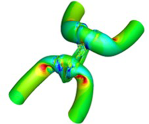
3.4. Vortex reconnection in orthogonally interacting tubes
We also simulate the interaction of two orthogonally offset vortex tubes in a periodic box of dimension  $2{\rm \pi}$ (Boratav et al. Reference Boratav, Pelz and Zabusky1992). The initial configuration is shown in figure 6. We specify vorticity along the axes of the tubes, specifically vorticity in ‘vortex Y’ is along the $-\hat {y}$ axis and vorticity in ‘vortex Z’ is along the $+\hat {z}$ axis. The compact Gaussian function, described previously in (3.7), distributes vorticity in the tube's cross-section. This ensures vorticity is non-zero only inside the tube of radius $r_c=0.666$. Both tubes have an initial circulation of $\varGamma =7.665$, and the Reynolds number based on circulation is set to $Re=1400$. As discussed previously, the velocity field is initialized by solving the Poisson equation (3.8).

Figure 6. Initial configuration for interaction of orthogonally offset tubes.
4. Local vortex line shapes in turbulent flows
The probability distribution of local vortex line shapes in turbulent flow fields generated from (i) randomly initialized isotropic field with large-scale forcing and (ii) Taylor–Green vortex field without any external forcing are investigated in detail in this section. The vortex line shapes are analysed in the framework of normalized vorticity gradient tensor invariants ( $q_\omega$, $r_\omega$). A comparison is drawn between the probability distributions of vortex line shapes in the two different turbulent flows.
4.1. Forced isotropic turbulence
The p.d.f. of  $\varPhi _{11}$ and its normalized component, $\chi _{11}$, for different $Re_\lambda$ are shown in figure 7. As expected, the tails of the p.d.f. of $\varPhi _{11}$ grow with increasing Reynolds number. Conversely, the p.d.f. of $\chi _{11}$ is bounded by definition and is compactly supported in the range described by (2.23). Importantly, the $\chi _{11}$ p.d.f. collapses to a self-similar shape for $Re_\lambda \geq 38$. Following the precedent of Das & Girimaji (Reference Das and Girimaji2020), vortex line shapes are analysed in the bounded invariant space of $\boldsymbol {\chi }$.

Figure 7. Marginal p.d.f. of the longitudinal component of the (a) un-normalized ( $\varPhi _{11}$) and (b) normalized ( $\chi _{11}$) vorticity gradient tensor.
The joint p.d.f.s of  $q_\omega$– $r_\omega$ in forced isotropic turbulent flows of different $Re_\lambda$ are plotted in figure 8. The dashed lines mark the realizable region of the $q_\omega$– $r_\omega$ plane. It is well known that the joint p.d.f. of velocity gradient tensor invariants ( $q$–
$q$– $r$) has a characteristic teardrop shape with maximum probability of occurrence along the right discriminant line of the plane (Das & Girimaji Reference Das and Girimaji2020). In contrast, the joint p.d.f. of $q_\omega$– $r_\omega$ shows that the highest probability of occurrence is at and around the origin of the plane, which represents straight parallel vortex lines. At $Re_\lambda =1$, the p.d.f. resembles that of a Gaussian field reflecting the random forcing of the flow field. As $Re_\lambda$ increases from $1$ to $25$ the region close to the origin becomes progressively more densely populated, which indicates an increase in probability of straight vortex lines in the flow. At $Re_\lambda =25$, the joint p.d.f. approaches its asymptotic shape. The characteristic form is symmetric in $r_\omega$ and resembles a ‘bell-like’ shape. In the next range of Reynolds numbers, i.e. for $Re_\lambda \in (25,225)$, the joint p.d.f. contours undergo finer refinements of this shape. At $Re_\lambda = 225$, the joint p.d.f. attains a self-similar shape and is invariant above this Reynolds number. This is demonstrated by superposing line contours in figure 8(i). It is evident that the joint p.d.f.s of $Re_\lambda =225,385$ and $588$ are nearly identical. This is similar to the findings of Das & Girimaji (Reference Das and Girimaji2019) for the $q$–
$q$– $r$ joint p.d.f., which also asymptotes to a self-similar shape at the same $Re_\lambda (= 225)$. It is further evident from figure 8 that from $Re_\lambda = 1$ to $86$ the joint p.d.f. shrinks closer to the origin, while from $Re_\lambda = 86$ to $225$ the p.d.f. expands away from the origin before it achieves a characteristic invariant distribution. The characteristic p.d.f. at $Re_\lambda \geq 225$ has the highest density near the origin and the densities decrease as we move away from the origin. This indicates a clear preference of turbulence to attain local vortex line shapes that are straight. This is in agreement with the findings of Boschung et al. (Reference Boschung, Schaefer, Peters and Meneveau2014). The p.d.f. in the plane further indicates that the focal topologies have a higher probability of occurrence in a turbulent flow field than non-focal vortex lines. For all the $Re_\lambda$ cases, the joint p.d.f. is more symmetric in $r_\omega$ than the velocity gradient case. The symmetry is more pronounced at higher Reynolds numbers. This symmetry indicates that vortex lines in a turbulent flow field are equally likely to be stable (converging towards a centre or a node) as unstable (diverging from a centre or a node). Such a symmetry is consistent with the observations of Wang (Reference Wang2012) in the distribution of positive and negative vortex line segments. Boschung et al. (Reference Boschung, Schaefer, Peters and Meneveau2014) also reported that the joint distribution of invariants of curvature tensor for local vortex lines is symmetric.

Figure 8. The  $q_\omega - r_\omega$ joint p.d.f. filled contour plots for $Re_\lambda$ = (a) $1$, (b) $6$, (c) $9$, (d) $14$, (e) $18$, (f) $25$, (g) $86$ and (h) $225$; (i) line contour plots for $Re_\lambda =86 - 588$.
The percentage of points in the turbulent flow field belonging to the four different vortex line topologies are plotted as a function of  $Re_\lambda$ in figure 9. The vortex line topology percentages do not show a strong dependence on Reynolds number. There is a noticeable variation in the fractions of SFS and UFC topologies only for $Re_\lambda \leq 25$. However, the sum total of the two focal topologies (SFS and UFC) and that of the two non-focal topologies (SN/S/S and UN/S/S) remain nearly constant at all Reynolds numbers. As inferred from the $q_\omega$– $r_\omega$ joint p.d.f., the focal topologies (SFS and UFC) indeed dominate over the non-focal topologies (SN/S/S and UN/S/S). The focal vortex lines occupy approximately $75\,\%$ of the flow field, while only $25\,\%$ of the field is constituted by non-focal vortex lines. At high Reynolds numbers ( $Re_\lambda \geq 86$), the symmetry of the probability distribution with respect to $r_\omega$ is further evident in figure 9, as the population fractions of stable and unstable topologies obtained are exactly equal.

Figure 9. Population fraction of non-degenerate vortex line topologies for forced isotropic turbulence at different  $Re_\lambda$.
The intermittency of velocity gradients has received much attention in previous works (Sreenivasan & Antonia Reference Sreenivasan and Antonia1997; Buaria et al. Reference Buaria, Pumir, Bodenschatz and Yeung2019). We now examine the intermittency of the vorticity gradients. A scatter plot of the extreme values of the velocity gradient tensor norm ( $\|A\|^{2}$) and vorticity gradient tensor norm ( $\|\varPhi \|^{2}$) is shown in figure 10. A few locations in the turbulent flow field have high values for both $\|A\|^{2}$ and $\|\varPhi \|^{2}$; however, there are also a significant number of points with high $\|\varPhi \|^{2}$ and low $\|A\|^{2}$ and vice versa. Nearly $45\,\%$ of points exhibit both high velocity and vorticity gradients.

Figure 10. Scatter plot for extreme values of  $\|\varPhi \|^{2}$ ( $>900$) and $\|A\|^{2}$ ( $>140$) for $Re_\lambda =225$.
Vorticity gradients are a higher order derivative than velocity gradients and representing statistics of a lower order quantity in a higher order space leads to a near uniform distribution much like the distribution of kinetic energy in a velocity gradient invariant space. Therefore, the intermittency of velocity gradients cannot be captured in the  $q_\omega - r_\omega$ space. However, the intermittency of vorticity gradients can be examined in the $q_\omega - r_\omega$ space. Toward this end, the conditional average of the Frobenius norm squared of the vorticity gradient tensor ( $\langle \|\varPhi \|^{2} | r_\omega , q_\omega \rangle$) is shown in figure 11(a). It is evident from the figure that the highest conditional average $\|\varPhi \|^{2}$ occurs at the origin indicating that straight vortex lines have the highest vorticity gradients on average. The conditional average of $\|\varPhi \|^{2}$ decreases away from the origin and is minimum at the boundaries of the $q_\omega - r_\omega$ plane. It may further be noted that the average vorticity gradient magnitude tends to be slightly higher for focal or spiraling vortex lines compared with the non-focal vortex line shapes. Next, the points of most intense vorticity gradient magnitudes ( $\|\varPhi \|^{2}>1000$) are marked in the $q_\omega ,r_\omega$ plane in figure 11(b). The scatter plot clearly suggests that these intense magnitude events are most likely to occur when the vortex lines are straight. There also appears to be a tendency for such high values to occur when vortex lines are nearly two-dimensional (2-D), i.e. $r_\omega \approx 0$.

Figure 11. (a) Conditional average of the Frobenius norm of the vorticity gradient tensor ( $\langle \varPhi ^{2}|r_\omega , q_\omega \rangle /\langle \varPhi ^{2}\rangle$) in the $q_\omega - r_\omega$ plane for $Re_\lambda =225$; (b) scatter plot of extreme vorticity magnitude ( $\|\varPhi \|^{2}>1000$) in the $q_\omega - r_\omega$ plane.
Overall, the local vortex line shape exhibits a characteristic bell shape that is invariant at sufficiently high Reynolds numbers. Vortex lines in a turbulent flow field are equally likely to be stable or unstable. Turbulence exhibits a strong preference for focal vortex lines over non-focal vortex lines. Further, the highest average vorticity gradient occurs in locally straight vortex lines.
4.2. Taylor–Green vortex breakdown
The joint p.d.f. distribution of  $q_\omega - r_\omega$ for the initial Taylor–Green field is plotted in figure 12(a). The initial p.d.f. is densely populated in two regions: (I) at the ordinate axis near $q_\omega =0.4$; and (II) at the intersection of the lower boundary and discriminant lines ( $q_\omega =-1/2, r_\omega = \pm 1/(3\sqrt {6}$)). The local vortex line shapes corresponding to region II are axisymmetric vortex expansion or axisymmetric vortex compression depending on the sign of $r_\omega$, whereas region I corresponds to vortex line shapes that are close to planar elliptic. We identify planes in the physical domain wherein the joint p.d.f. of that plane is concentrated in either region I or region II. The field vortex lines in such planes, derived from the vorticity field, are then plotted in figure 12(b–c). Figure 12(b) plots the vortex lines coloured by $q_\omega$ and figure 12(c) plots the same coloured by $r_\omega$. We observe that $q_\omega$ is positive and $r_\omega \approx 0$ for the elliptic vortex lines (region I). Similarly in region II, ( $q_\omega \approx -0.5, r_\omega >0$) for axisymmetrically expanding vortex lines and ( $q_\omega \approx -0.5, r_\omega <0$) for axisymmetrically compressing vortex lines. Therefore, the field vortex lines are in agreement with the shapes predicted by the $q_\omega$– $r_\omega$ classification framework.

Figure 12. (a) Filled contour plot of the  $q_\omega - r_\omega$ joint p.d.f. for the initial field of a Taylor–Green vortex flow. Field vortex lines in physical space dominated by regions I and II of the $q_\omega - r_\omega$ joint p.d.f. coloured by (b) $q_\omega$ (c) $r_\omega$.
We now present the evolution of the  $q_\omega$– $r_\omega$ joint p.d.f. as the flow starts breaking down toward turbulence. The initial field (figure 13a) is mostly constituted by vortex line shapes belonging to regions I and II of the $q_\omega$– $r_\omega$ plane as discussed above. The vortex line shapes belonging to region I, predominantly planar elliptic in nature, begin to change first, which results in a reduction of the p.d.f. values (figure 13b,c). These vortex line shapes are replaced by straight parallel vortex lines, as indicated by the emerging p.d.f. values near the origin (figure 13c,d). Following this, the region II (axisymmetrically expanding/compressing) vortex lines are replaced by locally straight vortex lines (figure 13d–f). At $t^{*} \approx 0.74$, the characteristic bell shape of the p.d.f. begins to materialize. Note that this happens quite early on in the timeline of breakdown to turbulence, well before the peak dissipation is achieved at $t^{*}=9.23$. The p.d.f. then undergoes further refinements and asymptotes to a self-similar form shortly after the peak of dissipation (figure 13g–i). We now compare the joint probability distribution of $q_\omega$– $r_\omega$ of the Taylor–Green vortex flow field after peak dissipation with that of the forced isotropic turbulent flow field at $Re_\lambda = 225$ and that of the turbulent channel flow at the $Re_\tau =5200$. The data for turbulent channel flow is obtained from Johns Hopkins Turbulence Database (Moser et al. Reference Moser, Kim and Mansour1999; Perlman et al. Reference Perlman, Burns, Li and Meneveau2007; Li et al. Reference Li, Perlman, Wan, Yang, Meneveau, Burns, Chen, Szalay and Eyink2008). The data at the wall-normal plane $y^{+}=100$ is considered in plotting the joint p.d.f. for the channel flow. The Taylor Reynolds number at the plane $y^{+}=100$ is $Re_\lambda =81$. The velocity derivatives in the joint p.d.f. computations are obtained with spectral accuracy in the streamwise and spanwise directions, while a fourth-order central difference scheme is used for the wall-normal derivative. As shown in figure 14, the p.d.f.s and the population percentages for the four vortex line topologies are nearly identical for all the flows. This indicates that the characteristic bell shape of the $q_\omega$– $r_\omega$ distribution is unique in turbulent flow fields much like the characteristic teardrop-shape distribution observed for the velocity gradient invariants.

Figure 13. The  $q_\omega - r_\omega$ joint p.d.f. filled contour plots for Taylor–Green vortex simulation at (a) $t^{*}=0$, (b) $t^{*}=0.132$, (c) $t^{*}=0.145$, (d) $t^{*}=0.160$, (e) $t^{*}=0.185$, (f) $t^{*}=0.740$, (g) $t^{*}=5$, (h) $t^{*}=9.23$ and (i) $t^{*}=11.57$.

Figure 14. The  $q_\omega - r_\omega$ joint p.d.f. line contour plots and population fractions of non-degenerate topologies for forced isotropic turbulence (FIT) at $Re_\lambda =225$, Taylor–Green vortex flow (TG) at $t^{*}=12$ (shortly after peak dissipation) and turbulent channel flow at $Re_\tau =5200$ on the wall-normal plane $y^{+}=100$. Data for the turbulent channel flow case are obtained from Johns Hopkins Turbulence Database (Moser, Kim & Mansour Reference Moser, Kim and Mansour1999; Perlman et al. Reference Perlman, Burns, Li and Meneveau2007; Li et al. Reference Li, Perlman, Wan, Yang, Meneveau, Burns, Chen, Szalay and Eyink2008).
5. Local vortex line shape in vortex reconnection
We now examine the local vortex line structure during the important process of vortex line reconnection. As mentioned in § 1, reconnection plays a key role in many flows of interest. In these flows, reconnection can occur between two vortices of different initial alignments. Here, we consider two canonical initial orientations previously studied in the literature and examine the reconnection process from the local vortex line shape point of view. The focus is primarily on the mechanism of bridging (Melander & Hussain Reference Melander and Hussain1988; Kida et al. Reference Kida, Takaoka and Hussain1991; Boratav et al. Reference Boratav, Pelz and Zabusky1992) in vortex reconnection.
5.1. Anti-parallel vortex tubes
We now examine the evolution of local vortex line shapes during vortex reconnection via bridging in sinusoidally perturbed anti-parallel vortex tubes. The key events leading up to and beyond bridging are traced by analysing the isosurfaces of vorticity magnitude at different instants of time in figure 15. The isosurfaces are coloured by  $q_\omega$ to track the evolution of local vortex line shapes during this period. We do not show results for $r_\omega$ as it is close to zero everywhere in the tubes at all times. This indicates that the local vortex lines are nearly 2-D and allows $q_\omega$ to completely characterize the local vortex line shape. The different steps in the vortex reconnection process and the corresponding vortex line shapes are discussed below with reference to figures 15–17.
(i) At
$t=0, q_\omega$ is zero everywhere on the surface, which indicates that the local vortex line shape is straight on the tube surface. In figure 16, we plot contours of $q_\omega$ in the symmetry ($x$–$y$) plane to describe the vortex line shapes in the tube's cross-section. Initially, the dominant vortex line shape in the tube's cross-section is straight, except for small regions near the core (red and blue crescent-shaped regions in figure 16a). In these particular regions, the curvature effects are dominant. Due to the strong curvature effects, the linearity assumption of determining local vortex line shapes from $q_\omega$–$r_\omega$ might not hold. As a result, the local vortex line shape is not necessarily reflective of the large-scale vortex line shape.(ii) The two tubes move toward each other by mutual induction and are pressed against each other at
$t=3.6$. At this stage, the cores of the tubes in the interaction region are significantly flatter. The vortex line shape is dominantly straight in the tubes everywhere excluding the contact region. The contact region comprises of positive values of $q_\omega$, which indicates locally elliptic vortex lines. The vortex line shapes in the contact region are examined in greater detail by the contours of $q_\omega$ in the cross-section of the contact zone shown in figure 16(b). The local vortex line shapes in the contact zone are dominantly planar elliptic as evident from the positive values of $q_\omega$.(iii) Cross-linking between the tubes results in annihilation of vorticity in the symmetry plane. Correspondingly, orthogonal vorticity emerges in the dividing plane resulting in vortex reconnection. By
$t=4.4$, reconnection is initiated and at the ends of the contact zone a hump connects the two tubes. The hump is called a bridge (Melander & Hussain Reference Melander and Hussain1988) and the process is termed vortex reconnection via bridging. Vortex line shapes inside the bridges are analysed by examining the contours of $q_\omega$ in the dividing plane in figure 17. The vortex line shapes inside the bridges are dominantly planar elliptic in the inner bridge portions, while planar hyperbolic vortex lines are prevalent in the outer bridge regions. Henceforth, this specific occurrence of paired vortex line shapes in the bridges will be referred to as ‘elliptic–hyperbolic pairing’. Aside from the bridges, the vortex line shapes everywhere else in the vortex tubes are mostly straight.(iv) The orthogonal transfer of vorticity from the tubes in the interaction region makes them weaker, and correspondingly the bridges become stronger. This is evident from figure 15(d), wherein the bridges have thickened and the interaction region has experienced thinning. At this stage the vortex line shapes in the curved region of the tubes are more elliptic. Moreover, as shown in figure 17(b), ‘elliptic–hyperbolic pairing’ continues to be the dominant vortex line shapes inside the bridges.
(v) As the bridges strengthen, self-induction causes the bridges to pull apart from the interaction region, stretching the remnant of tubes (threads) in the contact zone. The separation between the bridges has increased in figure 15(e). The distribution of vortex line shapes in the tubes is similar to that in figure 15(d).
(vi) At the final time step under consideration (figure 15f), the bridges have morphed to be part of the two vortex half-rings and the hump is indiscernible. The two formed vortex half-rings have elliptic vortex line shapes near the curved portions. The ‘elliptic–hyperbolic pairing’ is still the dominant vortex line topology inside the morphed bridges (figure 17c). Meanwhile, self-induction between the curved threads results in them moving away from each other. The corresponding vortex line shapes inside the threads (figure 16c) are also predominantly straight.


We now analyse the evolution of vortex line shapes in the vortex tubes altogether by examining the joint probability distribution of  $q_\omega - r_\omega$. We only consider points with vorticity magnitude greater than $30\,\%$ of the maximum initial vorticity in plotting such joint distributions (figure 18). Initially, the vortex line shape is locally straight (i.e. $q_\omega \approx r_\omega \approx 0$) almost everywhere. At $t=4.4$, i.e. at the inception of bridging, the joint p.d.f. has expanded along the $q_\omega$ axis while still remaining constrained in the $r_\omega$ axis. This implies that the local vortex line shapes are highly likely to be planar. In addition, the vortex line shapes are no longer restricted to only straight lines, rather they are very likely to be elliptic or hyperbolic in nature. Finally, by $t=6$, the likelihood of straight vortex lines has decreased further as more elliptic and hyperbolic vortex lines appear. This is partially due to the coiling of vortex lines (Van Rees, Hussain & Koumoutsakos Reference Van Rees, Hussain and Koumoutsakos2012) in the vortex half-rings.

Figure 15. The  $|\omega |$ isosurfaces at $30\,\%$ of maximum initial vorticity coloured by $q_\omega$ at t = (a) $0$, (b) $3.6$, (c) $4.4$, (d) $4.8$, (e) $5.4$ and (f) $6$.
$6$.

Figure 16. The  $q_\omega$ contours in the symmetry plane at $t=$ (a) $0$, (b) $3.6$ and (c) $6$. Contours are only shown in regions wherein $|\omega |>0.3\omega _0$.

Figure 17. The  $q_\omega$ contours in the dividing plane at $t=$ (a) $4.4$, (b) $4.8$ and (c) $6$. Contours are only shown in regions wherein $|\omega | > 0.3 \omega _0$.

Figure 18. The  $q_\omega - r_\omega$ joint p.d.f. filled contours at $t=$ (a) $0$, (b) $4.4$ and (c) $6$. Only points with $|\omega |>0.3\omega _0$ are considered.
5.2. Orthogonally interacting tubes
In this section we consider the reconnection of orthogonally offset vortex tubes. The evolution of isosurfaces of vorticity magnitude coloured by  $q_\omega$ at different stages leading up to and beyond reconnection of the tubes are shown in figure 19. Unlike the previous case of anti-parallel vortex tubes, there exist certain regions at the vortex tube surface wherein $r_\omega$ is non-zero, which suggests that the local vortex line shapes in such regions are not necessarily planar and likely to be 3-D. However, such regions are few and far between, and locally the vortex lines are predominantly 2-D at the surface of the tubes. The different stages of reconnection are described as follows with reference to figures 19–21.
(i) Initially, the local vortex lines are straight everywhere in the tubes. The vortex tubes move and deform under the influence of each other's velocity field. At
$t=2.64$, the local vortex line shape continues to be straight almost everywhere except for the highly curved regions in the vortex tube wherein it is elliptic as indicated by positive $q_\omega$ values.(ii) Vortex Z under the influence of the velocity field of vortex Y starts moving along the direction of it's binormal. This leads to the configuration as shown in figure 19(c) wherein the mid regions of the vortex tubes are parallel and the vorticity in the tubes is directed in opposite directions. The cores of the vortex tubes at the mid regions are flat and pressed against each other creating an ideal setting for reconnection via bridging. At this stage, the vortex line shapes in the tubes are dominantly straight except for the elliptic vortex lines in the curved regions of the tubes. As in the previous case of reconnection in anti-parallel vortex tubes, vortex line shapes in the contact region are also elliptic.
(iii) By
$t=4.92$, bridging is initiated and the ends of the contact regions are connected by bridges. The local vortex line shapes in the upper bridge surface are dominantly hyperbolic as indicated by negative values of $q_\omega$ there. We also plot contours of $q_\omega$ (figure 20) and $r_\omega$ (figure 21) in the dividing plane slicing through the bridges. At $t=5.16$, just after the onset of bridging, $q_\omega$ is dominantly negative in the outer region of bridges while it is positive in the inner regions. At this stage, the contours of $r_\omega$ shown in figure 21(a) demonstrate that even though $r_\omega$ is not exactly zero everywhere inside the bridges, it is very close to zero in the non-zero $q_\omega$ regions of the bridges. Therefore, in such regions the vortex line shapes are nearly planar and the dominant vortex line shape in the bridges is clearly constituted by ‘elliptic–hyperbolic pairing’.(iv) The sequence of events beyond bridging is similar to the anti-parallel case. Further annihilation of vorticity in the symmetry plane accompanied by generation of orthogonal vorticity in the dividing plane makes the bridges stronger, while simultaneously weakening the mid section of the tube (figure 19e). The vortex line shapes in the tubes in the bridges continue to show ‘elliptic–hyperbolic pairing’.
(v) By
$t=6$, the bridges have integrated with the tubes and the hump is indiscernible. Self-induction has pushed the bridges away from each other consequently stretching the mid sections of the tubes into slender threads. At this stage, the vortex line shapes at the surface of the reconnected tubes are mostly straight lines barring the highly curved regions of the tubes wherein elliptic vortex lines occur. Overall, the vortex line shapes in the reconnected region are still dominated by ‘elliptic–hyperbolic pairing’ (figure 20c).


Finally, we plot the joint p.d.f. of  $q_\omega - r_\omega$ in figure 22 to examine the vortex line shapes in the entire vortex tubes. Initially, the joint p.d.f. is entirely centred at the origin as the vortex lines are exclusively straight in the tubes. At $t=5.16$, beyond bridging, the joint p.d.f. has expanded away from the origin albeit being dominantly constrained near the $q_\omega$ axis implying planar shapes are highly likely. At late times more 3-D shapes appear as the joint p.d.f. contours expand away from the origin. The sequence of events leading up to and beyond vortex reconnection via bridging in this case are similar to the anti-parallel case. Additionally, in both the cases a specific configuration of elliptic and hyperbolic vortex lines are prominent in the bridges. This leads us to conclude that the emergence of this ‘elliptic–hyperbolic pairing’ in the bridges is independent of the initial orientation of the vortex tubes.

Figure 19. The  $|\omega |$ isosurfaces at $40\,\%$ of maximum initial vorticity coloured by $q_\omega$ at t = (a) $0$, (b) $2.64$, (c) $4.32$, (d) $4.92$, (e) $5.28$ and (f) $6$.
$6$.

Figure 20. The  $q_\omega$ contours in the dividing plane at $t=$ (a) $5.16$, (b) $5.28$ and (c) $6$. Contours are only shown in regions wherein $|\omega |>0.4\omega _0$.

Figure 21. The  $r_\omega$ contours in the dividing plane at $t=$ (a) $5.16$, (b) $5.28$ and (c) $6$. Contours are only shown in regions wherein $|\omega |>0.4\omega _0$.

Figure 22. The  $q_\omega - r_\omega$ joint p.d.f. filled contours $t=$ (a) $0$, (b) $5.16$ and (c) $6$. Only points with $|\omega |>0.4\omega _0$ are considered.
6. Summary and conclusions
The paper seeks to characterize infinitesimal vortex line topology by adapting the local streamline topology classification method of Chong et al. (Reference Chong, Perry and Cantwell1990). The differences between velocity and vorticity fields are identified and the critical point analysis is suitably modified. Topology classification in terms of second and third invariants of the vorticity gradient tensor is reiterated and the invariant evolution equations are derived. Vortex line geometry classification, which is related to topology, is introduced using suitably normalized vorticity gradient invariants (Das & Girimaji Reference Das and Girimaji2019). An extensive investigation of vortex line geometry distribution in forced isotropic turbulence is conducted over a wide range of Reynolds numbers. Specifically, the joint p.d.f. of the second and third normalized vorticity gradient invariants ( $q_\omega$– $r_\omega$) is examined. At very low Reynolds numbers (order unity), the joint p.d.f. form is similar to that of a Gaussian field. With increasing Reynolds number, the p.d.f. form changes and attains self-similarity beyond $Re_\lambda > 200$. It was shown by Das & Girimaji (Reference Das and Girimaji2019) that the joint p.d.f. of normalized velocity gradient invariants also attains self-similarity beyond $Re_\lambda > 200$. The high-Reynolds-number vorticity gradient invariants’ p.d.f. is of symmetric bell shape with the highest probability density at locally parallel vortex lines. Moreover, it is shown that straight vortex lines have the highest average vorticity gradient magnitude. The topology and geometry distribution during Taylor–Green vortex breakdown toward turbulence is next examined. Initially, the flow field is constituted of only two specific vortex line geometric shapes. With time the flow deforms and convolutes the vortex lines, which creates smaller scales of motion. Consequently, the vortex line elements of different topologies and geometric shapes are generated. The joint p.d.f. of $q_\omega$– $r_\omega$ gradually takes the characteristic bell shape seen in forced isotropic turbulence. This finding suggests that that the bell-shape distribution is likely a universal characteristic of turbulence across different types of turbulent flows analogous to the teardrop shape of the velocity gradient invariants’ joint p.d.f. The study next examines the vortex reconnection phenomenon, specifically the bridging process that initiates the merger. Different initial vortex tube configurations are considered. It is demonstrated the structure of vortex filaments inside the bridges in both cases considered are distributed in a similar fashion. The bridge is constituted of 2-D elliptic vortex lines on one side and hyperbolic vortex lines on the other.
Acknowledgements
The authors would like to thank Professor D. Donzis of Texas A&M University for providing the DNS data of forced isotropic turbulence used in this study. Portions of this research were conducted with the advanced computing resources provided by Texas A&M High Performance Research Computing.
Declaration of interest
The authors report no conflict of interest.
Appendix A
In the present work, the vorticity vector is given by  $\boldsymbol {\omega }$ and the vorticity gradient tensor is given by
 \begin{equation} \varPhi_{ij} = \frac{\partial \omega_i}{\partial x_j}. \end{equation}
It is demonstrated in § 2 that the local vortex line can be classified into distinct topologies and its shape can be completely defined by the normalized second and third invariants of  $\boldsymbol {\varPhi }$.
In a recent work by Boschung et al. (Reference Boschung, Schaefer, Peters and Meneveau2014), vortex line topology was studied in terms of curvature and rotation of a surface element normal to the vorticity vector. Toward this end, they first define a unit vector in the direction of vorticity,
 \begin{equation} t_i = \frac{\omega_i}{\mid\boldsymbol{\omega}\mid}. \end{equation}
They further define a curvature tensor,
 \begin{equation} {\mathsf{T}}_{ij} = \frac{\partial t_i}{\partial x_j}. \end{equation}
This tensor is different from the vorticity gradient tensor and is related to  $\varPhi _{ij}$ as follows:
 \begin{equation} {\mathsf{T}}_{ij} = \frac{1}{\mid\boldsymbol{\omega}\mid}\left( \varPhi_{ij} - t_i \frac{\partial \omega_i}{\partial x_j} \right). \end{equation}
The tensor  ${\mathsf{T}}_{ij}$ has two non-zero invariants – first ( $H$) and second ( $K$), while the third invariant is zero, since the third eigenvalue of ${\mathsf{T}}_{ij}$ is zero by construction. In contrast, $\varPhi _{ij}$ has the first invariant zero by definition, while the second ( $Q_\omega$) and third ( $R_\omega$) invariants are used to determine the vortex line geometry.
The main principle behind the work of Boschung et al. (Reference Boschung, Schaefer, Peters and Meneveau2014) is that the real parts of the two non-zero eigenvalues of  ${\mathsf{T}}_{ij}$ determine the curvature of a surface element perpendicular to the unit vorticity vector ( $t_i$), while the imaginary parts represent the rotation of such a surface. This surface curvature in turn provides certain information about the local change of $t_i$ and therefore the vortex line tangential to it. Based on this, they have characterized different surface element topologies and the corresponding 2-D configurations of the vortex lines in the phase space of $H$ and $K$ (see figure 2 of Boschung et al. Reference Boschung, Schaefer, Peters and Meneveau2014). This provides important information about the converging or diverging nature of the local vortex lines. However, it does not determine the complete 3-D shape of the vortex lines.
In the present work, we analyse the geometry of the local vortex lines directly based on the local vorticity gradient tensor, following the work of Chong et al. (Reference Chong, Perry and Cantwell1990). This enables us to characterize the complete 3-D shape of the local vortex lines in the compact phase space of  $q_\omega$ and $r_\omega$ (§ 2.5). It is evident that the present framework provides details about the vortex line shapes that are not amenable to the surface element based analysis of Boschung et al. (Reference Boschung, Schaefer, Peters and Meneveau2014).
Appendix B
In a frame of reference rotating with angular velocity  $\varOmega$, the local vorticity ( $\boldsymbol {\omega }_R$) field is related to the inertial vorticity field by
 \begin{equation} \boldsymbol{{\omega}}_R=\boldsymbol{\omega}-2\boldsymbol{\varOmega}. \end{equation}
We select a coordinate frame rotating with angular velocity  $\boldsymbol {\varOmega }=\boldsymbol {\omega }(\boldsymbol {x}_0)/2$. In such a frame the local vorticity field ( $\boldsymbol {\omega }_R$) is given by the following equation:
 \begin{equation} \boldsymbol{{\omega}}_R=\boldsymbol{\omega}-\boldsymbol{\omega}(\boldsymbol{x}_0). \end{equation}
The local vorticity in such a frame is the same as the ‘relative vorticity field’  $\boldsymbol {\tilde {\omega }}(\boldsymbol {x};\boldsymbol {x}_0)$ as defined in (2.15). We now derive equations for vortex lines in the rotating frame of reference. Vortex lines as observed from a rotating frame of reference are curves tangent to the local vorticity in the rotating frame. We denote by $x_i'$ the basis of the rotating frame whereas $x_i$ represents the inertial basis. Similarly, $(\omega _R')_i$ denotes the components of local vorticity vector along the rotating basis and $(\omega _R)_i$ denotes the components of vorticity in the rotating frame expressed along the inertial basis. At time $t$, the coordinate basis $x_i$ can be transformed to $x_i'$ by a proper rotation. Let $\boldsymbol{\mathsf{Q}}$ be an orthogonal coordinate transformation tensor such that
 \begin{equation} {\mathsf{Q}}_{ij}=\frac{\partial x_i'}{\partial x_j}. \end{equation}
The transformation tensor  $\boldsymbol{\mathsf{Q}}$ obeys the standard transformation rules transforming vectors between the two bases $x_i$ and $x_i'$ as follows:
 \begin{equation} (\omega_R')_i={\mathsf{Q}}_{im}(\omega_R)_m. \end{equation}
In a rotating frame, the differential equation governing vortex lines is as follows:
 \begin{equation} \frac{\textrm{d} x_i'}{\textrm{d} s}=(\omega_R')_i. \end{equation}
We multiply (B5) by  ${\mathsf{Q}}_{im}$ to cast it along the inertial basis:
 \begin{equation} \frac{\textrm{d} x_m}{\textrm{d} s}=(\omega_R)_m, \end{equation}
where we have used (B3) and the transformation identity for vectors (B4). Solution trajectories obtained by integrating (B6) for a frozen vorticity field are vortex lines as observed in a rotating frame of reference.
Since  $\boldsymbol {\tilde {\omega }}(\boldsymbol {x};\boldsymbol {x_0})$ and $\boldsymbol {\omega }_R$ are the same by definition, (B6) and (2.16) are identical. Thus, the so-called ‘relative vortex lines’ are indeed the vortex lines observed from a frame rotating with angular velocity $\boldsymbol {\omega }(\boldsymbol {x}_0)/2$.


 Open access