


Impact Statement
Thermoacoustic instabilities can affect a wide array of combustion technologies. Combustors suffering from such instabilities would be a major safety hazard as they would be extremely loud and inefficient, could become structurally compromised, or could even explode. Predicting the occurrence of thermoacoustic instabilities early in the design process is thus crucial to avoid expensive mitigation strategies at later development stages. Thermoacoustic stability prediction is usually performed using physics-based modeling and simulations. In this study, an alternative methodology based on classification algorithms is shown to be much more efficient at predicting the occurrence of combustion instabilities while still being highly accurate. Optimizing the properties of combustors at the design stage could thus be made much faster by using this methodology.
1. Introduction
Thermoacoustic instabilities, also called combustion instabilities, occur due to a positive feedback loop between an unsteady heat source and the surrounding acoustic waves (Rayleigh, Reference Rayleigh1878; Poinsot and Veynante, Reference Poinsot and Veynante2001; Dowling and Stow, Reference Dowling and Stow2003). They can occur in a variety of industrial and domestic combustors such as rocket and aircraft engines (Crocco, Reference Crocco1951;Candel, Reference Candel2002; Lieuwen and Yang, Reference Lieuwen and Yang2005; Poinsot, Reference Poinsot2017), land-based gas turbines (Candel, Reference Candel2002; Lieuwen and Yang, Reference Lieuwen and Yang2005; Poinsot, Reference Poinsot2017), boilers (Putnam, Reference Putnam1971; Eisinger and Sullivan, Reference Eisinger and Sullivan2002), and many other types of combustors. Combustion instabilities are usually undesirable as they can cause flame extinction or flashback (Candel, Reference Candel1992; Poinsot, Reference Poinsot2017), structural damage (Candel, Reference Candel1992; McManus et al., Reference McManus, Poinsot and Candel1993; Poinsot, Reference Poinsot2017), and increased sound emissions (Schuller et al., Reference Schuller, Durox and Candel2003; Poinsot, Reference Poinsot2017), among other adverse effects.
Many rocket engines from the 1950s and 1960s suffered from thermoacoustic instabilities, thus driving a major research effort to predict and control the occurrence of such instabilities (Crocco, Reference Crocco1951; Merk, Reference Merk1957; Crocco et al., Reference Crocco and Grey1960). Combustion instabilities were investigated using experiments and analytical models since computers of that era were unable to run complex numerical simulations. These traditional approaches were only partially successful, and predicting the thermoacoustic stability of a given configuration at the design stage remained essentially out of reach (Harrje and Reardon, Reference Harrje and Reardon1972). Interest in thermoacoustics research dwindled in the following decades, until a new generation of low-NOx gas turbines, prone to thermoacoustic instabilities, was introduced in the early 1990s (Correa, Reference Correa1993; Keller, Reference Keller1995; Paschereit and Polifke, Reference Paschereit and Polifke1998; Dowling and Morgans, Reference Dowling and Morgans2005). Rapid developments in experimental techniques and numerical capacities opened the door to a range of new strategies for studying combustion instabilities, including computational fluid dynamics (CFD) simulations (Veynante and Poinsot, Reference Veynante and Poinsot1997; Poinsot and Veynante, Reference Poinsot and Veynante2001; Polifke et al., Reference Polifke, Poncet, Paschereit and Döbbeling2001; Xia et al., Reference Xia, Laera, Jones and Morgans2019), low-order models (Keller, Reference Keller1995; Paschereit and Polifke, Reference Paschereit and Polifke1998; Dowling and Stow, Reference Dowling and Stow2003; Li and Morgans, Reference Li and Morgans2015; Nair and Sujith, Reference Nair and Sujith2015; Xia et al., Reference Xia, Laera, Jones and Morgans2019; Gaudron et al., Reference Gaudron, Yang and Morgans2020; Fournier et al., Reference Fournier, Haeringer, Silva and Polifke2021), or hybrid methods (Kaess et al., Reference Kaess, Polifke, Poinsot, Noiray, Durox, Schuller and Candel2008; Silva et al., Reference Silva, Nicoud, Schuller, Durox and Candel2013; Li et al., Reference Li, Yang, Luzzato and Morgans2017; Ni et al., Reference Ni, Miguel-Brebion, Nicoud and Poinsot2017; Merk et al., Reference Merk, Silva, Polifke, Gaudron, Gatti, Mirat and Schuller2018). Next-generation combustors burning carbon-free fuels, such as hydrogen or ammonia, appear to show increased propensity to combustion instabilities (Æsøy et al., Reference Æsøy, Aguilar, Bothien, Worth and Dawson2021; Beita et al., Reference Beita, Talibi, Sadasivuni and Balachandran2021; Lim et al., Reference Lim, Li and Morgans2021). Being able to accurately determine the thermoacoustic stability of combustors will thus become even more critical as the fossil fuel era nears its end.
Predicting the thermoacoustic stability of combustors remains a challenging task as of today. CFD simulations are computationally expensive because of the large range of space and timescales associated with the acoustic waves and flame unsteadiness that need to be resolved (Poinsot and Veynante, Reference Poinsot and Veynante2001; Merk et al., Reference Merk, Silva, Polifke, Gaudron, Gatti, Mirat and Schuller2018). Physics-based low-order network model tools are more computationally efficient (Paschereit and Polifke, Reference Paschereit and Polifke1998; Dowling and Stow, Reference Dowling and Stow2003), but the roots of one complex characteristic equation need to be determined for every configuration investigated (Dowling and Stow, Reference Dowling and Stow2003; Gaudron et al., Reference Gaudron, Yang and Morgans2020). Since optimizing a combustor at the design stage requires a large amount of configurations to be considered, low-order network models may become relatively computationally expensive (Jones et al., Reference Jones, Gaudron and Morgans2021). In recent years, Machine Learning algorithms have been increasingly employed to detect the onset of combustion instabilities in burners (Murugesan and Sujith, Reference Murugesan and Sujith2015; Murugesan and Sujith, Reference Murugesan and Sujith2016; Sarkar et al., Reference Sarkar, Chakravarthy, Ramanan and Ray2016; Kobayashi et al., Reference Kobayashi, Murayama, Hachijo and Gotoda2019; McCartney et al., Reference McCartney, Indlekofer and Polifke2020; Sujith and Unni, Reference Sujith and Unni2020). However, those algorithms are essentially time series predictors that can predict the immediate future (no more than a few seconds) by making use of physical signals such as the unsteady pressure in the combustion chamber (Murugesan and Sujith, Reference Murugesan and Sujith2015; Sarkar et al., Reference Sarkar, Chakravarthy, Ramanan and Ray2016; McCartney et al., Reference McCartney, Indlekofer and Polifke2020). Those algorithms are thus not capable of predicting the thermoacoustic stability of a given configuration at the design stage.
Another category of Machine Learning algorithms that do not take physical time series as inputs could be used to discriminate between stable and unstable configurations without actually assembling them. One such category is that of classification algorithms, that typically run very quickly and could thus be used to design stable combustors efficiently. The objective of this work is to test this conjecture by determining whether well-established classification algorithms are able to predict the thermoacoustic stability of combustors with various geometries and flame properties. Four different algorithms are investigated: the K-Nearest Neighbors (KNN; Fix and Hodges, Reference Fix and Hodges1951; Altman, Reference Altman1992), Decision Tree (DT; Breiman et al., Reference Breiman, Friedman, Olshen and Stone1984; Quinlan, Reference Quinlan1986), Random Forest (RF; Ho, Reference Ho1995; Breiman, Reference Breiman2001), and Multilayer Perceptron (MLP; Hinton, Reference Hinton1989; Haykin, Reference Haykin1998) algorithms. A very large number of labeled configurations is first generated using a physics-based low-order network tool in order to train and validate those algorithms, as described in Section 2. The overall thermoacoustic stability of those randomly generated combustors is then predicted using the binary KNN, DT, RF, and MLP algorithms in Section 3, and the corresponding accuracy scores and runtimes are assessed. Finally, the frequency range is split into 10 smaller frequency intervals, and the thermoacoustic stability of the previous configurations is predicted in each frequency interval using the multilabel KNN, DT, RF, and MLP algorithms in Section 4. The accuracy scores, training runtimes, and prediction runtimes are also assessed for all four multilabel classification algorithms.
2. Generation of the Synthetic Data
Classification algorithms need to be trained with a large number of examples before they can accurately predict the label of an unknown case. It is impossible to obtain enough data by running experiments because it would require every single geometry to be designed, built, and investigated. CFD is also not an option as hundreds of thousands of simulations would need to be run, which would have an exorbitant computational cost. The solution adopted in this study is to use a low-order network tool, OSCILOS, that represents combustors as networks of connected modules. OSCILOS is an open-source code written in MATLAB and developed at Imperial College London. OSCILOS can predict the thermoacoustic stability of a given burner by solving one-dimensional flow conservation equations. It has been shown to accurately predict the frequencies and growth rates of thermoacoustic modes appearing in a variety of combustors at a moderate computational cost (Han et al., Reference Han, Li and Morgans2015; Li et al., Reference Li, Yang, Luzzato and Morgans2017; Xia et al., Reference Xia, Laera, Jones and Morgans2019; Gaudron et al., Reference Gaudron, Yang and Morgans2020). More information about OSCILOS, including the equations that are used to describe each type of module, can be found in Li et al. (Reference Li, Yang, Luzzato and Morgans2017) and Gaudron et al. (Reference Gaudron, MacLaren and Morgans2021).
OSCILOS was used to generate a large number of cases corresponding to random geometries and flame properties and determine their corresponding thermoacoustic stability. The combustor’s geometry for each case contains four sections: the inlet, Interfaces 1 and 2, and the outlet, thus corresponding to three distinct modules. The inlet is located at x = 0 m, and the axial locations of the remaining sections are randomly generated between x = .1 m and x = 1 m. The radii of all three modules are also randomly generated between r = .01 m and r = .1 m. The flame is always located at the second interface, and its frequency response is represented using an n–τ model (Merk, Reference Merk1957; Poinsot and Veynante, Reference Poinsot and Veynante2001; Lieuwen, Reference Lieuwen2005). Modern predictive approaches often use computational flow simulations to deduce the flame’s frequency response, but an n–τ model captures the main features at a much-reduced computational cost. For each case, the gain and time delay of the n–τ model are also randomly selected in the range $ n\in \left[.5,1\right] $
and
$ n\in \left[.5,1\right] $
and $ \tau \in \left[0,5\right] $
ms. All random parameters are selected using a uniform distribution. An example of a geometry generated using this procedure is depicted in the top of Figure 1.
$ \tau \in \left[0,5\right] $
ms. All random parameters are selected using a uniform distribution. An example of a geometry generated using this procedure is depicted in the top of Figure 1.
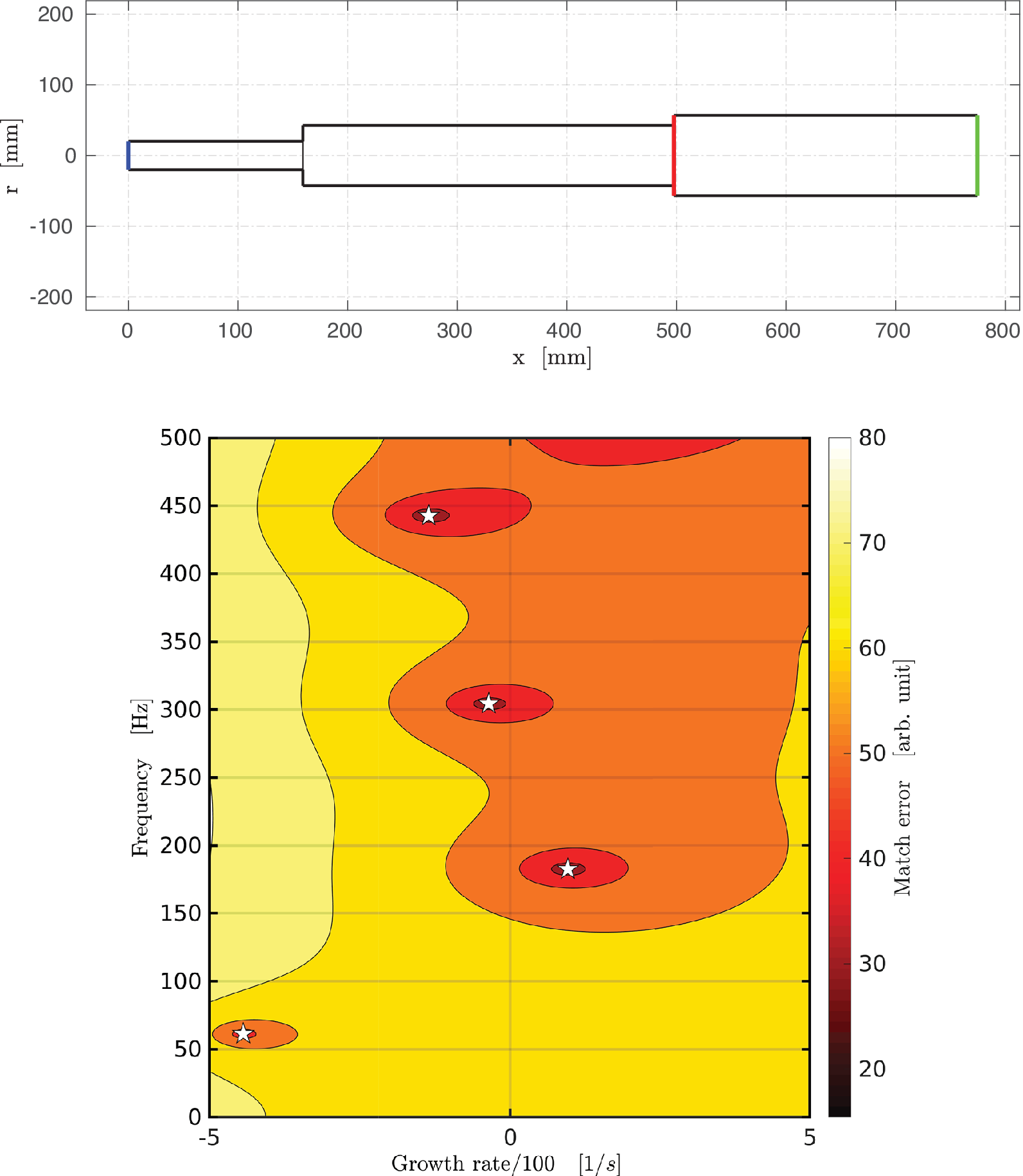
Figure 1. (Top) Randomly generated combustor geometry consisting of three modules with a flow passing through from left to right. The axial locations of the inlet, flame, and outlet are depicted by blue, red, and green vertical lines, respectively. (Bottom) Corresponding map obtained using OSCILOS with n = .875 and τ = 4.90 ms. A white star indicates the presence of a thermoacoustic mode for that frequency and growth rate.
The mean pressure, mean temperature, and Mach number at the inlet are then set to $ {p}_0=101,325 $
Pa,
$ {p}_0=101,325 $
Pa, $ {T}_0=293 $
K, and
$ {T}_0=293 $
K, and $ {M}_0=.005 $
for all cases. Likewise, the mean temperature ratio across the flame is always set to 5. The mean flow parameters are then computed everywhere inside the combustor by solving the mean conservation of mass, momentum, and energy. For all cases, the acoustic boundary conditions at the inlet and the outlet are set to a closed
$ {M}_0=.005 $
for all cases. Likewise, the mean temperature ratio across the flame is always set to 5. The mean flow parameters are then computed everywhere inside the combustor by solving the mean conservation of mass, momentum, and energy. For all cases, the acoustic boundary conditions at the inlet and the outlet are set to a closed $ \left({\mathcal{R}}_i=1\right) $
and open (
$ \left({\mathcal{R}}_i=1\right) $
and open ( $ {\mathcal{R}}_o=-1 $
) end, respectively. A characteristic equation is then solved, and all thermoacoustic modes with a frequency within
$ {\mathcal{R}}_o=-1 $
) end, respectively. A characteristic equation is then solved, and all thermoacoustic modes with a frequency within $ f\in \left[0,500\right] $
Hz and a growth rate within
$ f\in \left[0,500\right] $
Hz and a growth rate within $ \omega \in \left[-500,500\right] $
s−1 are detected. For instance, the bottom of Figure 1 represents the map corresponding to the geometry depicted in the top of Figure 1 with a gain n = .875 and a time delay τ = 4.90 ms. Four thermoacoustic modes of frequencies f
1 = 61 Hz, f
2 = 183 Hz, f
3 = 304 Hz, and f
4 = 443 Hz are found for those parameters, represented in the bottom of Figure 1 as white stars.
$ \omega \in \left[-500,500\right] $
s−1 are detected. For instance, the bottom of Figure 1 represents the map corresponding to the geometry depicted in the top of Figure 1 with a gain n = .875 and a time delay τ = 4.90 ms. Four thermoacoustic modes of frequencies f
1 = 61 Hz, f
2 = 183 Hz, f
3 = 304 Hz, and f
4 = 443 Hz are found for those parameters, represented in the bottom of Figure 1 as white stars.
The original frequency range is then divided into 10 bins covering 50 Hz each, for example, the first and second bins cover the frequencies $ f\in \left[0,50\right] $
Hz and
$ f\in \left[0,50\right] $
Hz and $ f\in \left[50,100\right] $
Hz, respectively. For a given configuration, if there are one or more practically unstable modes, then a positive label (+1) is associated with the bin(s) containing the frequencies of those modes. Conversely, a naught label (0) is associated with all remaining bins, which can thus contain practically stable modes or no mode at all. A thermoacoustic mode is linearly stable for any negative growth rate (Poinsot and Veynante, Reference Poinsot and Veynante2001; Dowling and Stow, Reference Dowling and Stow2003; Lieuwen, Reference Lieuwen2005). However, a small change in the flow conditions and/or flame properties can alter the growth rate of a given mode (Langhorne, Reference Langhorne1988; Lieuwen, Reference Lieuwen2005) which could potentially shift from a slightly negative value to a positive value. The corresponding thermoacoustic mode would then become linearly unstable and grow in amplitude. For that reason, a practically unstable (respectively, stable) mode is defined as a mode with a growth rate
$ f\in \left[50,100\right] $
Hz, respectively. For a given configuration, if there are one or more practically unstable modes, then a positive label (+1) is associated with the bin(s) containing the frequencies of those modes. Conversely, a naught label (0) is associated with all remaining bins, which can thus contain practically stable modes or no mode at all. A thermoacoustic mode is linearly stable for any negative growth rate (Poinsot and Veynante, Reference Poinsot and Veynante2001; Dowling and Stow, Reference Dowling and Stow2003; Lieuwen, Reference Lieuwen2005). However, a small change in the flow conditions and/or flame properties can alter the growth rate of a given mode (Langhorne, Reference Langhorne1988; Lieuwen, Reference Lieuwen2005) which could potentially shift from a slightly negative value to a positive value. The corresponding thermoacoustic mode would then become linearly unstable and grow in amplitude. For that reason, a practically unstable (respectively, stable) mode is defined as a mode with a growth rate $ \omega >-20 $
s−1 (respectively,
$ \omega >-20 $
s−1 (respectively, $ \omega \le -20 $
s−1).
$ \omega \le -20 $
s−1).
As an illustration, the labels for the configuration presented in Figure 1 are reported in Table 1. Even though four thermoacoustic modes are found in the frequency range of interest, only the second mode has a growth rate $ \omega >-20 $
s−1. Since the frequency of this mode is f
2 = 183 Hz, the label associated with the fourth frequency interval is set to 1, whereas all the remaining labels are set to 0. The procedure described in this section is fully automated and takes a few seconds to run on a recent computer for any given configuration. In this study, hundreds of thousands of randomly generated configurations have been explored to train and validate the classification algorithms presented in Sections 3 and 4.
$ \omega >-20 $
s−1. Since the frequency of this mode is f
2 = 183 Hz, the label associated with the fourth frequency interval is set to 1, whereas all the remaining labels are set to 0. The procedure described in this section is fully automated and takes a few seconds to run on a recent computer for any given configuration. In this study, hundreds of thousands of randomly generated configurations have been explored to train and validate the classification algorithms presented in Sections 3 and 4.
Table 1. Labels associated with the randomly generated configuration introduced in Figure 1.

3. Binary Classification Algorithms
The first step is to try and predict the overall thermoacoustic stability of a given configuration by using binary classification algorithms. The code used to perform the corresponding analysis is available on GitHub as a Jupyter notebook. It is written in Python 3 and makes use of the scikit-learn library (Pedregosa et al., Reference Pedregosa, Varoquaux, Gramfort, Michel, Thirion, Grisel, Blondel, Prettenhofer, Weiss, Dubourg, Vanderplas, Passos, Cournapeau, Brucher, Perrot and Duchesnay2011). The inputs (also called features) are the lengths (L 1, L 2, L 3) and radii (R 1, R 2, R 3) of all three modules as well as the gain n and time delay τ of the flame model. The output is a binary value: 0 if the configuration contains no practically unstable mode for the entire frequency range of interest or 1 otherwise. Following this definition, the synthetic data presented in Section 2 contain 149,701 stable configurations (output: 0) and 401,656 unstable configurations (output: 1). The complexity of the classification problem is linked to the shape of the boundary separating stable and unstable configurations in the eight-dimensional feature space. Figure 2 depicts this boundary projected on the (n, τ) space for nine random sets of geometrical parameters (L 1, L 2, L 3, R 1, R 2, R 3). It is clear from Figure 2 that stable and unstable configurations are not always separable by simple lines, which implies that nonlinear algorithms are required for this classification task.
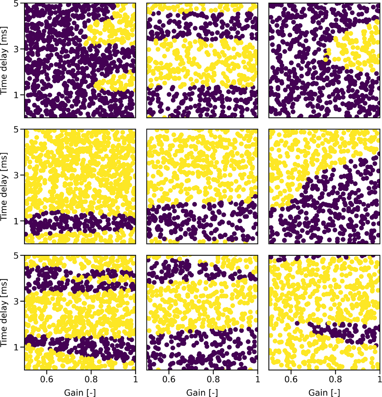
Figure 2. Thermoacoustic stability predicted by OSCILOS as a function of the time delay (y-axis) and gain (x-axis) of the flame for nine randomly generated combustor geometries. (Purple dots) Stable configurations. (Yellow dots) Unstable configurations.
The Kendall rank correlation coefficients between the inputs and the binary output are represented in Figure 3. These coefficients indicate that there is a very low correlation between all inputs (except for the time delay) and the binary output. In other words, those inputs have a very little impact on the thermoacoustic stability of combustors when considered separately. Conversely, there is a moderate positive correlation between the time delay and the binary output, thus indicating that configurations with higher time delays τ tend to be more thermoacoustically unstable.
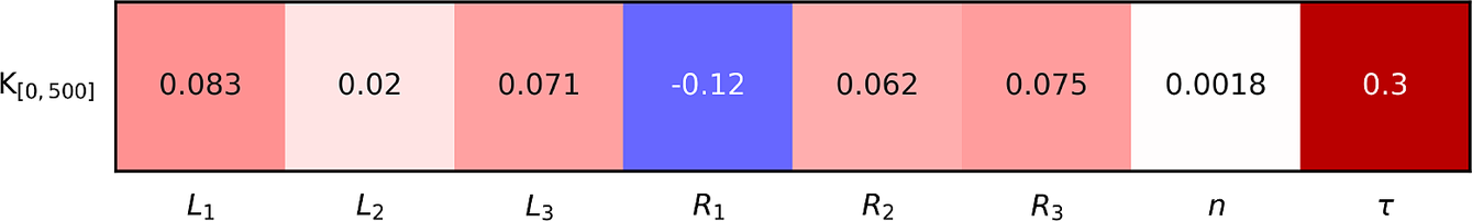
Figure 3. Kendall rank correlation coefficients between the inputs (x-axis) and the binary output.
An input matrix of dimension 551,357 × 8 is then constructed by assigning each feature to a column, while each row represents a different configuration. Every column of the input matrix is then normalized by removing the mean and scaling to unit variance. An output vector containing the binary output for every configuration is also constructed. The input matrix and the output vector are then split randomly into a training/cross-validation set and a testing set. The training/cross-validation set, which contains 80% of all configurations, is used to train the algorithms and tune the associated hyperparameters, whereas the testing set, which contains the remaining 20%, is used to validate the algorithms. These two sets are disjoint to ensure that training and testing are independent. The scoring metric used in this study is the Accuracy Classification Score, which quantifies the number of correctly labeled configurations. A fivefold cross-validation strategy is used to find the optimal value of the hyperparameters. This “training, tuning, testing” procedure is now described in detail. For a given algorithm, the training/cross-validation set is randomly split into five subsets of similar size. Four of these subsets, constituting the training set, are used to fit the model for given hyperparameters, whereas the fifth subset, called the cross-validation set, is used to compute the corresponding accuracy score. This operation is then repeated four times by selecting a different cross-validation set among the five subsets, and the average cross-validation accuracy score is then computed for those hyperparameters. The entire procedure is then repeated for another set of hyperparameters. The hyperparameters maximizing the average cross-validation accuracy score are then selected, and the algorithm is refit using the entire training/cross-validation set. The accuracy score of the refit model is finally assessed using the testing set. An illustration of the different subsets used for training, cross-validation, and testing is represented in Figure 4.
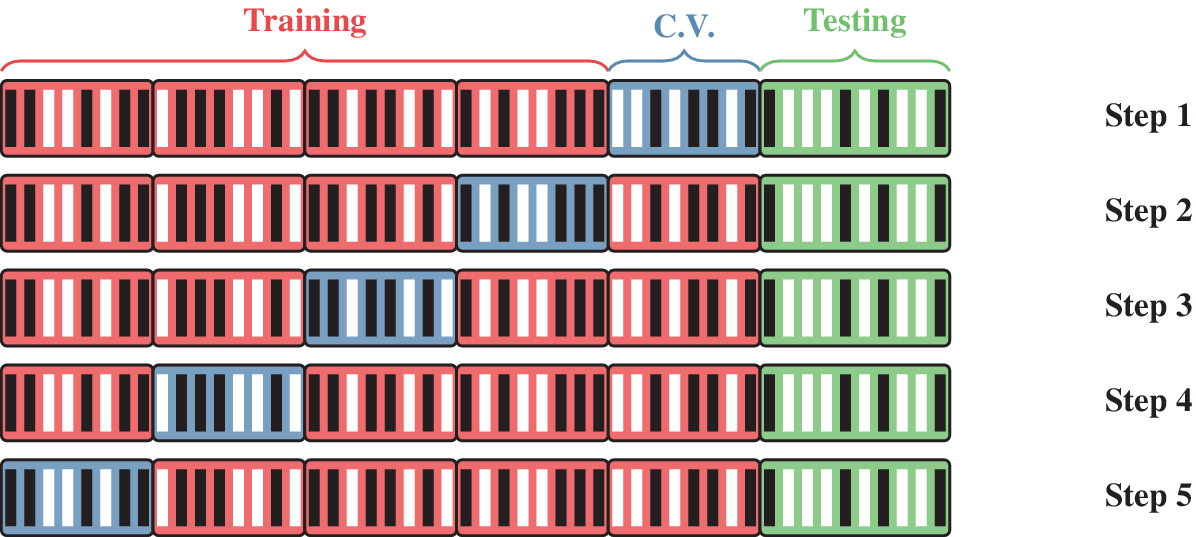
Figure 4. Illustration of the different subsets used in the fivefold cross-validation strategy for 50 randomly generated configurations of class 0 (black line) or 1 (white line). (Red) Training set. (Blue) Cross-validation set. (Green) Testing set.
The first binary classification algorithm investigated is the K Nearest Neighbors (KNN) algorithm (Fix and Hodges, Reference Fix and Hodges1951; Altman, Reference Altman1992), which assigns the class of an unknown configuration based on the most common class among its K nearest neighbors in the eight-dimensional feature space. The distance metric used in the feature space is the Minkowski distance, and the most appropriate algorithm (BallTree or KDTree) is automatically selected to compute the nearest neighbors. All configurations in a given neighborhood are weighted equally. The only hyperparameter of the KNN algorithm in this study is the number of neighbors K, varied between 1 and 50. The resulting average accuracy score computed using the cross-validation subsets is represented in the top of Figure 5 as a function of the number of neighbors. The top of Figure 5 shows that the accuracy score tends to decrease as the number of neighbors in the neighborhood increases. The best model is thus obtained for a single neighbor and yields a 99.3% accuracy when computed on the testing set after being refit on the entire training/cross-validation set.
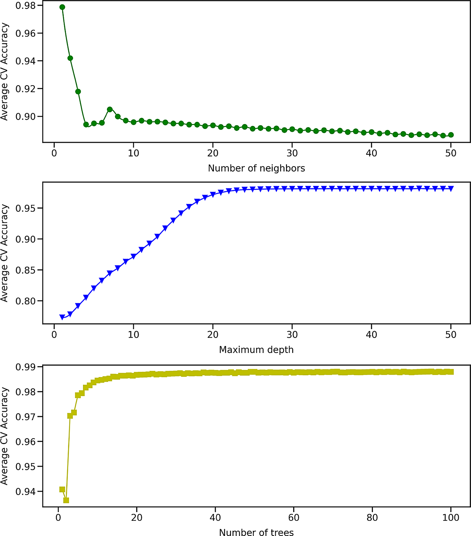
Figure 5. Average cross-validation accuracy score obtained using 440,086 training examples for the binary K-Nearest Neighbors (Top), Decision Tree (Middle), and Random Forest (Bottom) algorithms as a function of the number of neighbors, maximum depth, and number of trees, respectively.
The second binary classification algorithm investigated is the Decision Tree (DT) algorithm (Breiman et al., Reference Breiman, Friedman, Olshen and Stone1984; Quinlan, Reference Quinlan1986), which assigns the class of an unknown configuration using simple decision rules inferred from the data features. An example of a decision rule for a one-layer decision tree could be: “If the time delay τ is larger than a, then the class of that configuration is 1.” An additional layer can then be added by splitting the tree into two branches according to another decision rule. A split of the decision tree is selected if it is the best available split based on an information gain criterion and if it decreases the overall impurity (or entropy) of the tree. All features are taken into account when considering a split, and both classes are weighted equally. The maximum number of layers (also called maximum depth) of the decision tree is considered as a hyperparameter in this study, with values ranging from 1 to 50. The average cross-validation accuracy score is represented in the middle of Figure 5 as a function of the maximum depth of the decision tree. Initially, the accuracy score increases linearly with the maximum depth of the tree, until it reaches a plateau for a maximum depth of about 25 layers. The best accuracy score is obtained for a maximum depth of 43 layers and yields a 99.4% accuracy when computed on the testing set after being refit on the entire training/cross-validation set.
The third binary classification algorithm is the Random Forest (RF) algorithm (Ho, Reference Ho1995; Breiman, Reference Breiman2001), which trains multiple decision trees and assigns the class of an unknown configuration based on the most commonly predicted class by those trees. Decision trees used in the DT and RF algorithms have similar properties, except that they have no maximum depth in the latter case. Bootstrap samples are used when building trees, and both classes are weighted equally. The maximum number of trees in the forest is varied between 1 and 100. The average cross-validation accuracy score is represented in the bottom of Figure 5 as a function of the number of trees in the forest. Initially, the accuracy score increases sharply with the number of trees. For more than 20 trees, the accuracy score is marginally improved as the forest grows. The best accuracy score for the testing set is found to be 99.6% for 92 trees in the forest.
The fourth and final classification algorithm is the Multilayer Perceptron (MLP) algorithm, which is a type of feedforward artificial neural network (Hinton, Reference Hinton1989; Haykin, Reference Haykin1998). Several architectures were tested, and the best accuracy was obtained using three hidden layers containing 100 neurons each, corresponding to a large number of weights to be optimized during the training procedure. The activation function used for hidden layers is the rectified linear unit function. The log-loss function is optimized using a stochastic gradient-based optimizer (Kingma and Ba, Reference Kingma and Ba2017) with 10,000 epochs. Six different learning rates are investigated: .0001, .0003, .001, .003, .006, and .01. The size of minibatches is set to 200, and samples are shuffled in each iteration. The exponential decay rate for estimates of the first and second moment vectors are set to β
1 = .9 and β
2 = .999, respectively. The numerical stability parameter is set to $ \unicode{x03B5} ={10}^{-8} $
. A regularization term is added to the loss function to prevent overfitting. Several values for the corresponding regularization parameter are explored: .001, .003, .01, .03, .1, and .3. If 10 successive epochs do not meet the tolerance, set to 10−4, then convergence is considered to be reached and the MLP training is stopped. Using the fivefold cross validation strategy, the best values for the learning rate and regularization parameter are both found to be .001. The corresponding accuracy score computed using the refit model and the testing set is 98.2%.
$ \unicode{x03B5} ={10}^{-8} $
. A regularization term is added to the loss function to prevent overfitting. Several values for the corresponding regularization parameter are explored: .001, .003, .01, .03, .1, and .3. If 10 successive epochs do not meet the tolerance, set to 10−4, then convergence is considered to be reached and the MLP training is stopped. Using the fivefold cross validation strategy, the best values for the learning rate and regularization parameter are both found to be .001. The corresponding accuracy score computed using the refit model and the testing set is 98.2%.
So far, the binary classification algorithms have been assessed using 551,357 configurations, of which 440,086 were training examples. In a practical setting, significantly less data might be available, thus affecting the accuracy of those classification algorithms. Figure 6 depicts the average cross-validation accuracy score as a function of the number of training examples for all four binary classification algorithms tuned with the optimal hyperparameters determined earlier. The performance of the KNN, DT, and RF algorithms are strongly affected as the training set shrinks, whereas the MLP algorithm is more robust. For training sets containing less than about 315,000 training examples, the best classification algorithm is the MLP algorithm. Above that threshold, the RF algorithm performs increasingly better. This is illustrated in Figure 7 where the maximum accuracy obtained using the testing set is represented for binary classification models trained using 220,043 and 440,086 labeled configurations. In the latter case, the best algorithm is indeed the RF algorithm, with only four mislabeled configurations for every 1,000 cases, closely followed by the DT and KNN algorithms with, respectively, six and seven mistakes for every 1,000 cases. Conversely, the MLP algorithm is less accurate (18 mistakes for every 1,000 cases). However, when the size of the training set is halved, the MLP algorithm features an accuracy of 96.8% as opposed to 95.6% for the RF algorithm, 93.5% for the DT algorithm, and 92.7% for the KNN algorithm.
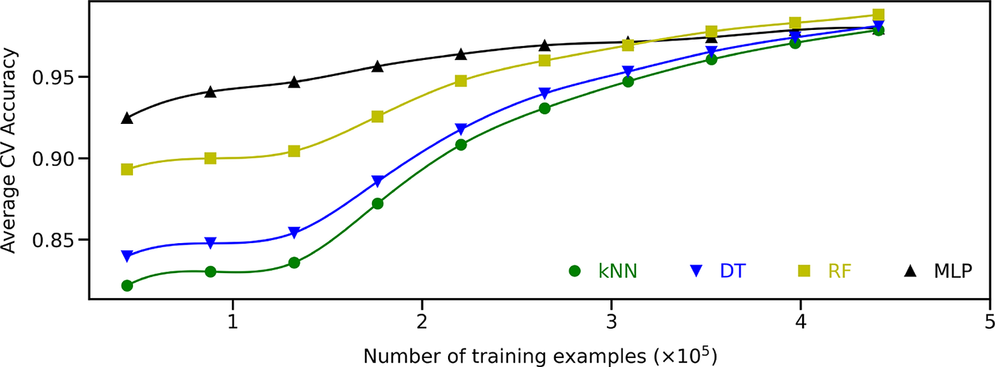
Figure 6. Average cross-validation accuracy score for the binary K-Nearest Neighbors (green dots), Decision Tree (blue triangles facing down), Random Forest (yellow squares), and Multilayer Perceptron (black triangles facing up) algorithms as a function of the number of training examples.
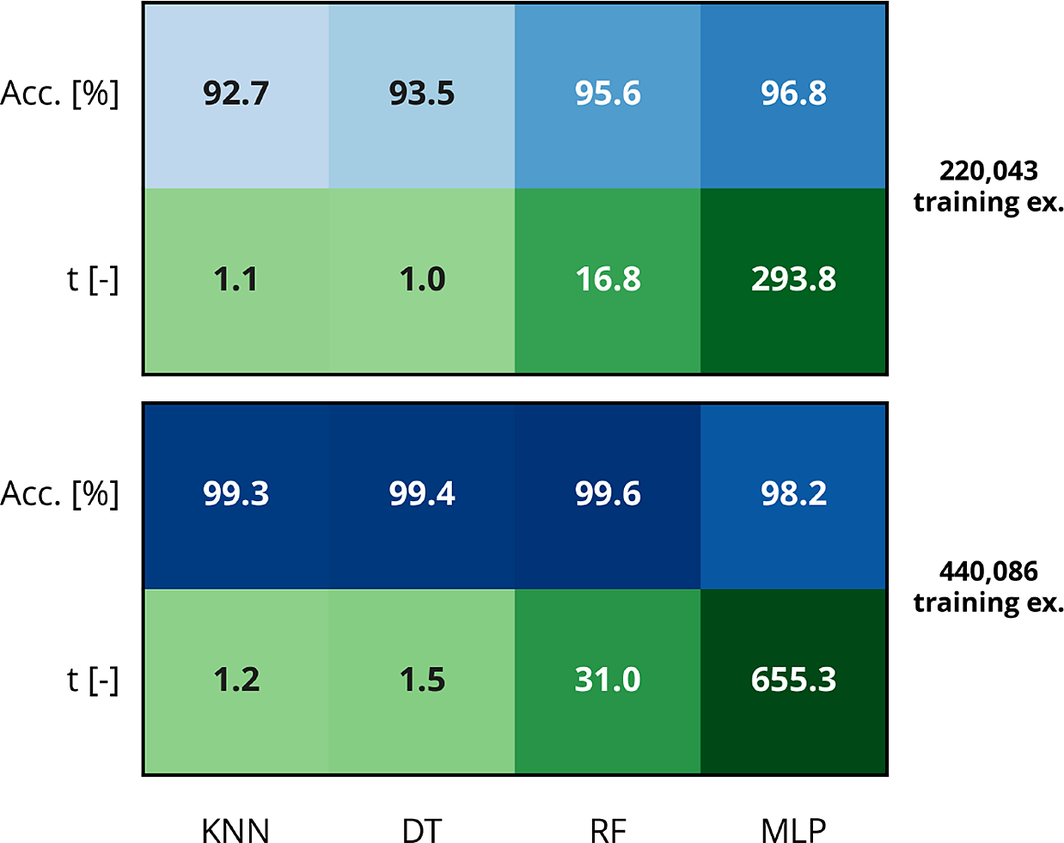
Figure 7. Maximum accuracy score obtained using the testing set (top row—blue) and training runtime of the corresponding model (bottom row—green) for various binary classification algorithms and for 220,043 (top) and 440,086 (bottom) training examples.
Figure 7 also indicates that the KNN and DT algorithms have similar training runtimes, whereas training the RF and MLP algorithms is 15–25 times slower and 300–600 times slower, respectively. Interestingly, doubling the size of the training set has a little impact on the training runtime of the KNN algorithm, whereas that of the DT algorithm increases by about 50% and those of the RF and MLP algorithms are approximately doubled.
4. Multilabel Classification Algorithms
The next step is to try and predict the thermoacoustic stability of a given configuration for the 10 distinct frequency intervals introduced in Section 2 (as opposed to the entire frequency range of interest). A given configuration is said to be correctly labeled if the labels of all 10 frequency intervals, covering 50 Hz each, are correctly predicted. In other words, the occurrence of practically unstable modes must be correctly predicted for every frequency interval. A given configuration may contain 0 positive label (no practically unstable mode in the entire frequency range), 10 positive labels (presence of at least one practically unstable mode in every frequency interval), or anything in between. The ratios of positive labels for the different frequency intervals are represented in Figure 8. Practically unstable modes are uncommon for frequencies f < 100 Hz, corresponding to the first two frequency intervals. The presence of at least one practically unstable mode is detected in about 10–15% of all configurations for the remaining frequency intervals. The Kendall rank correlation coefficients between the inputs and all 10 binary outputs are represented in Figure 9. Again, those correlation coefficients are either close to zero, or slightly positive or negative. This demonstrates that none of the inputs are good thermoacoustic stability predictors per se: they need to be considered collectively instead.
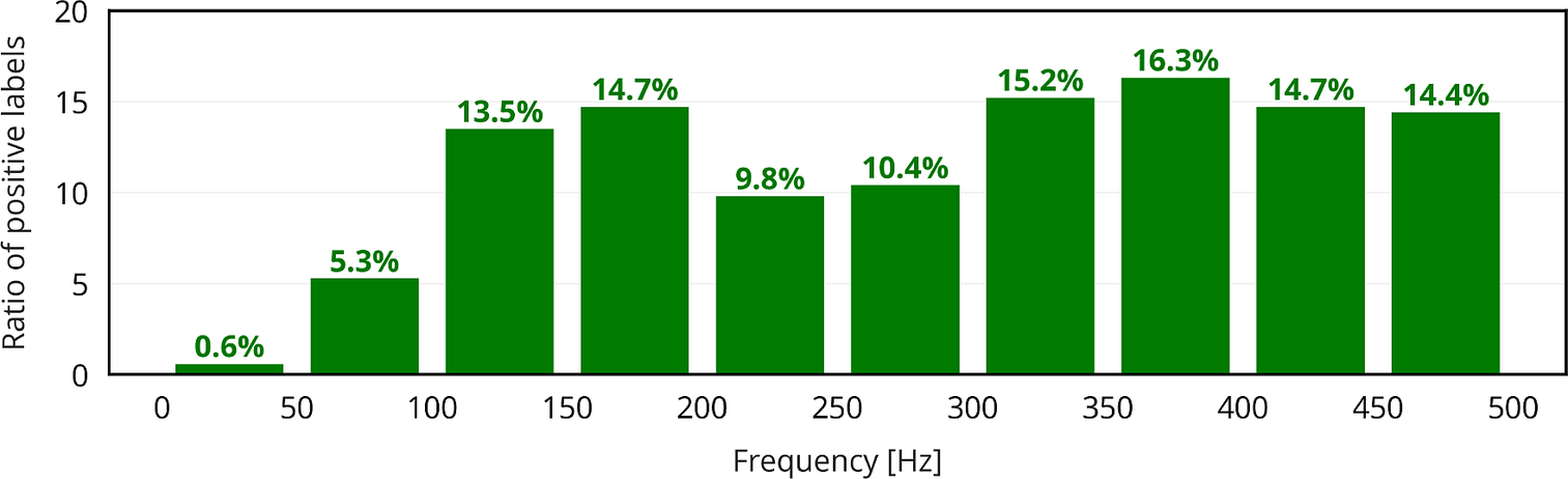
Figure 8. Ratios of positive labels for the different frequency intervals.
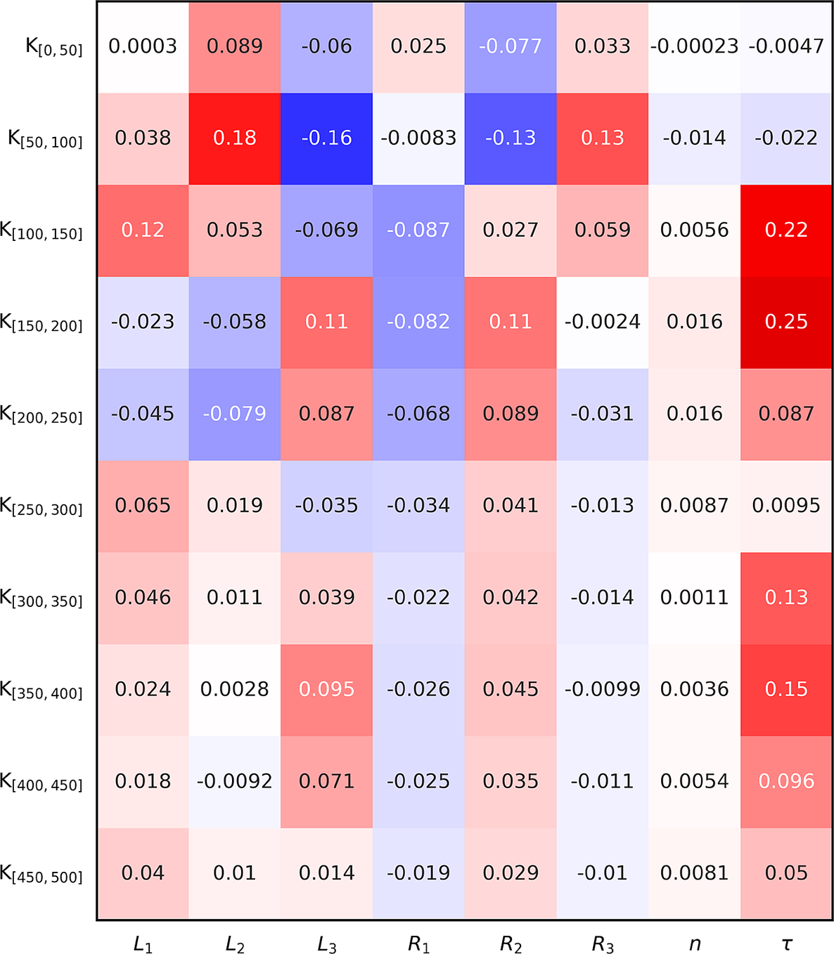
Figure 9. Kendall rank correlation coefficients between the inputs (x-axis) and the binary outputs (y-axis) corresponding to 10 distinct frequency intervals.
The KNN, DT, RF, and MLP algorithms are transformed into multilabel classification algorithms by using a classifier chain. First, the label corresponding to the first frequency interval (covering the frequencies between 0 and 50 Hz) is predicted based on the usual eight inputs (lengths and radii of the modules and flame parameters). The output of this first model is then added to the inputs, and a second model is trained to predict the label of the second frequency interval (covering the frequencies between 50 and 100 Hz). The second label is then added to the inputs, and so on, until all 10 models are trained. Using a classifier chain instead of training 10 independent models based on the same eight inputs was found to lead to a higher accuracy score. For each multilabel algorithm, the corresponding parameters are similar to those selected for their binary counterparts. Furthermore, the preprocessing procedure as well as the fivefold cross-validation strategy are also identical in both cases. As a first step, 440,086 labeled configurations are used to train the multilabel classification algorithms.
The average cross-validation accuracy score for the multilabel KNN algorithm is represented as a function of the number of neighbors in the top of Figure 10. As observed for the binary KNN algorithm, the accuracy score decreases when the number of neighbors increases. For a single neighbor, the testing accuracy achieved after refitting the model using the entire cross-validation/training set is 97.5%. Similarly, the average cross-validation accuracy scores for the multilabel DT and RF algorithms are represented in the middle and the bottom of Figure 10 as functions of the maximum depth of the tree and the number of trees in the forest, respectively. The trend that was first detected for the binary DT and RF algorithms, that is, a sharp increase followed by a plateau, is observed once again. The most accurate models are obtained for a maximum depth of 50 layers and a forest containing 85 trees for the DT and RF algorithms, respectively. The corresponding accuracy scores of the refit models assessed using the testing set is 97.7% for the DT algorithm and 98.3% for the RF algorithm. Finally, the multilabel MLP algorithm is found to be most accurate for the same learning rate and regularization parameter that were selected for the binary MLP algorithm: .001. The corresponding testing accuracy of the refit model is 94.2%. Figure 11 demonstrates that the RF algorithm is indeed the most accurate multilabel algorithm for a training/cross validation set containing more than about 370,000 training examples. The multilabel MLP algorithm is more robust and thus becomes the most accurate multilabel algorithm for a smaller number of training examples. This can also be observed in Figure 12, which represents the accuracy scores of all four multilabel algorithms as well as the corresponding training runtimes for 220,043 and 440,086 training examples. Figure 12 further shows that the multilabel KNN and DT algorithms have similar training runtimes, whereas training the multilabel RF and MLP algorithms is 15–20 times slower and 200–300 times slower, respectively. Finally, doubling the size of the training set is found to have a little impact on the training runtime of the multilabel KNN algorithm, but increases that of the DT algorithm by about 60% and nearly doubles those of the RF and MLP algorithms. These observations closely follow those made for binary classification algorithms in Section 3.

Figure 10. Average cross-validation accuracy score obtained using 440,086 training examples for the multilabel K-Nearest Neighbors (top), Decision Tree (middle), and Random Forest (bottom) algorithms as a function of the number of neighbors, maximum depth, and number of trees, respectively.

Figure 11. Average cross-validation accuracy score for the multilabel K-Nearest Neighbors (green dots), Decision Tree (blue triangles facing down), Random Forest (yellow squares), and Multilayer Perceptron (black triangles facing up) algorithms as a function of the number of training examples.

Figure 12. Maximum accuracy score obtained using the testing set (top row—blue) and training runtime of the corresponding model (bottom row—green) for various multilabel classification algorithms and for 220,043 (top) and 440,086 (bottom) training examples.
A classification algorithm with carefully selected parameters only needs to be trained once if the training examples cover a wide enough range of inputs. This initial step has a low-to-moderate computational cost depending on the specific algorithm, but the resulting model can then predict the labels of a previously unknown configuration within those predefined bounds very efficiently. It should also be noted that the training and prediction steps can be performed on different machines. This is a major advantage of classification algorithms compared to traditional low-order network tools, where a single step of moderate computational cost is required to make a prediction. This is illustrated in Figure 13, where the labels associated with 10,000 configurations are predicted using multilabel KNN, DT, RF, and MLP algorithms as well as OSCILOS. The classification algorithms are pretrained using 440,086 labeled configurations. The fastest pretrained algorithm is the DT algorithm, followed by the MLP and RF algorithms that run about 22 and 67 times slower. The slowest multilabel classification algorithm, the KNN algorithm, is 114 times slower than the DT algorithm. Nevertheless, OSCILOS is still several orders of magnitudes slower than the KNN algorithm. Astonishingly, the DT algorithm is able to make a prediction about the thermoacoustic stability of a given configuration almost a million times faster than OSCILOS.

Figure 13. Prediction runtime for 10,000 distinct configurations obtained using various multilabel classification algorithms and OSCILOS.
5. Conclusions
Thermoacoustic instabilities are a major issue in the power production and aircraft propulsion industries, among many others. The development and widespread adoption of new carbon-free combustion technologies could be hindered as they are especially prone to combustion instabilities. It is possible to predict the occurrence of those combustion instabilities using complex physical models and/or numerical simulations. However, optimizing the properties of a given combustor to make it instability-proof requires dozens of thousands of runs, and the associated computational cost may become quite high. Conversely, classification algorithms typically run much faster, but have never been used for thermoacoustic stability prediction. The objective of this work was thus to investigate whether a selection of well-established classification algorithms could be trained to accurately predict the thermoacoustic stability of combustors with arbitrary geometries and flame properties.
Over half a million configurations were randomly generated and scanned for unstable thermoacoustic modes using a physics-based open-source tool called OSCILOS. Four binary classification algorithms of increasing complexity were then selected: the KNN, DT, RF, and MLP algorithms. After being trained using all available training examples, all four algorithms were shown to be capable of predicting the overall thermoacoustic stability of an unknown configuration with an accuracy higher than 98%. The most accurate algorithm was found to be the RF algorithm, with an accuracy score of 99.6%. It was then demonstrated that the MLP algorithm was the most accurate algorithm for smaller training sets. Finally, the KNN and DT algorithms were found to have lower accuracies than the RF algorithm and/or the MLP algorithm, but could be trained significantly faster.
Efficient mitigation strategies are highly dependent on the frequency of thermoacoustic instabilities. It is thus important to predict not only the occurrence of thermoacoustic instabilities, but also the frequency interval in which they occur. This was achieved in this study by considering multilabel classification algorithms. The frequency range of interest was split into 10 frequency intervals covering 50 Hz each, and the ith label was set to be positive if there was at least one unstable mode corresponding to the ith frequency interval. The thermoacoustic stability of a given configuration was considered to be correctly predicted if all 10 frequency intervals were correctly labeled. All four algorithms trained using all available training examples were found to have an accuracy score higher than 94%. The most accurate multilabel algorithm investigated was the RF algorithm with more than 98.3% of perfectly labeled configurations. Again, the MLP algorithm was found to be the most accurate algorithm for smaller training sets, and the KNN and DT algorithms were slightly less accurate, but could be trained much faster than the other two algorithms. Finally, it was shown that all trained multilabel classification algorithms were able to predict the thermoacoustic stability of an unknown configuration with runtimes several orders of magnitude smaller than that of a traditional low-order network tool. For instance, the DT algorithm, which was found to be the fastest multilabel classification algorithm, ran almost a million times faster than OSCILOS.
This study demonstrates that classification algorithms are able to predict the thermoacoustic behavior of a randomly generated configuration with a very high accuracy and a very low runtime. The frequency intervals in which unstable thermoacoustic modes appear can also be accurately predicted using multilabel classification algorithms. These findings open the door to a new generation of ML-based combustor optimization codes that would run much faster than the existing physics-based codes.
Data Availability Statement
The data and code that support the findings of this study are openly available at https://github.com/RenaudGaudron/Thermo_classification. OSCILOS is openly available on its official website at https://www.oscilos.com/.
Author Contributions
Conceptualization: R.G. and A.S.M.; Data curation: R.G.; Funding acquisition: A.S.M.; Methodology: R.G. and A.S.M.; Software: R.G.; Visualization: R.G.; Writing—original draft: R.G.; Writing—review & editing: A.S.M. All authors approved the final submitted draft.
Funding Statement
The authors would like to gratefully acknowledge the European Research Council (ERC) Consolidator Grant AFIRMATIVE (2018–2023), grant number 772080, for supporting this research.
Competing Interests
The authors declare none.


 Open access
Comments
No Comments have been published for this article.