


In this chapter, we outline our principles of text selection and preparation and then describe the statistical and computational methods we employ throughout this book. Each description includes a working example to demonstrate the method.
Text Selection and Preparation
Appendix A lists the full-text corpus of plays we use throughout this book, along with their authors (where known), dates of first performance, the source text we use, its date of publication, and its genre. We depart from our main bibliographical source, the second edition of the Annals of English Drama, 975–1700 (hereafter ‘Annals’), only where new research is persuasive and sound, as with the attribution of Soliman and Perseda to Thomas Kyd.Footnote 1
To construct our corpus of machine-readable (that is, electronic) texts, we have relied upon base transcriptions from Literature Online, checked and corrected against facsimiles from Early English Books Online. Since our analysis concerns word frequency and distribution, and not orthography, spelling was regularised and modernised. For the sub-set of plays used in Chapter 6, this was done using VARD, a software tool developed by Alistair Baron for regularising variant spelling in historical corpora.Footnote 2 Spelling was modernised, but early modern English word forms with present tense -eth and -est verb-endings (e.g. liveth and farest) were retained. For the larger sets of plays utilised in Chapters 2 and 7, we regularised spelling using a function in the Intelligent Archive software to combine variant forms with their headwords.Footnote 3 In all texts used, function words with homograph forms – such as the noun and verb form of will – were tagged to enable distinct counts for each. Appendix E lists the function words used in our analysis. Contractions were also expanded, such that where appropriate ‘Ile’ was expanded as an instance of I and one of willverb, ‘thats’ as an instance of thatdemonstrative and one of is, and so on.
Unless otherwise specified, texts are segmented into non-overlapping blocks of words – typically 2,000 words – with the last block, if incomplete, discarded to ensure consistent proportions. Proper names, passages in foreign languages, and stage directions are also discarded.Footnote 4 It is standard practice in authorship attribution testing to exclude proper names and foreign-language words from the analysis, because these are more closely related to local, play-specific contexts rather than indicative of any consistent stylistic pattern. As for stage directions, Paul Werstine has demonstrated that their status as authorial or non-authorial cannot be assumed, but varies from text to text.Footnote 5 We deemed it safer to exclude stage directions as a general rule rather than attempt to assess every instance.
Principal Components Analysis
Principal Components Analysis, or PCA, is a statistical procedure used to explain as much of the total variation in a dataset with as few variables as possible. This is accomplished by condensing multiple variables that are correlated with one another,Footnote 6 but largely independent of others, into a smaller number of composite ‘factors’.Footnote 7 The strongest factor or ‘principal component’ is the one that accounts for the largest proportion of the total variance in the data. PCA produces the strongest factor (the ‘first principal component’), and then the factor that accounts for the greatest proportion of the remaining variance while also satisfying the condition that it is uncorrelated with the first principal component – a property which we can visualise in a two-dimensional example as being at right-angles to it. Since each principal component only ever represents a proportion of the underlying relationships between the variables, PCA is a data reduction method. The method is also considered ‘unsupervised’, because it does not rely upon any human pre-processing of the data – the algorithm treats all of the samples equally and indifferently.Footnote 8
A classic example of how PCA is used to reduce the dimensions of multivariate data involves taking a table of the heights and weights of a group of people from which a new composite factor – which we might call ‘size’ – is generated as the sum of the two variables.Footnote 9 ‘Size’ will represent the patterns of variation within the two original variables with a high proportion of accuracy – shorter people will tend to be lighter, and taller people heavier – but it will not account for all the possible variations in height and weight, since some short people will be heavy and some taller people light. As a principal component, ‘size’ still captures a basic fact about the relationship between height and weight, one that, in a sense, is the most important. If we add two variables, say, waist size and muscle mass, a new first principal component may be calculated to account for the strongest correlation between all four variables, on the same principle of accounting for most of the variation by weighing the best-coordinated variables similarly. In this scenario, waist size and weight together may represent a proxy for ‘obesity’, and muscle mass and weight together may represent a proxy for ‘muscularity’, and so on.
As noted in the Introduction, PCA has been widely adopted as a method for stylistic investigation.Footnote 10 Its use in authorship attribution relies on the fact that, when analysing word-frequency counts across a mixed corpus of texts known to be of different authorship, the strongest factor that emerges in the relationship between the texts is generally authorial in nature. Other stylistic signals may also be present, such as the effect of genre, period of composition, gender of the author, and so on, but these are usually demonstrably weaker. For example, Table 1.1 lists a selection of plays by John Lyly, Christopher Marlowe, Thomas Middleton, and William Shakespeare, representing a range of genres and dates of first performance.Footnote 11
Table 1.1 A select corpus of plays
| Author | Play | Date |
|---|---|---|
| Lyly, John | Campaspe | 1583 |
| Lyly, John | Endymion | 1588 |
| Lyly, John | Galatea | 1585 |
| Lyly, John | Mother Bombie | 1591 |
| Marlowe, Christopher | 1 Tamburlaine the Great | 1587 |
| Marlowe, Christopher | 2 Tamburlaine the Great | 1587 |
| Marlowe, Christopher | Edward the Second | 1592 |
| Marlowe, Christopher; others (?) | The Jew of Malta | 1589 |
| Middleton, Thomas | A Chaste Maid in Cheapside | 1613 |
| Middleton, Thomas | A Mad World, My Masters | 1605 |
| Middleton, Thomas | A Trick to Catch the Old One | 1605 |
| Middleton, Thomas | Your Five Gallants | 1607 |
| Shakespeare, William | The Comedy of Errors | 1594 |
| Shakespeare, William | Richard the Third | 1592 |
| Shakespeare, William | The Taming of the Shrew | 1591 |
| Shakespeare, William | The Two Gentlemen of Verona | 1590 |
With this corpus of machine-readable texts, prepared as outlined above, we use Intelligent Archive, a software tool developed by the Centre for Literary and Linguistic Computing at the University of Newcastle, to generate word-frequency counts for the 500 most frequent words across the corpus, segmented into 2,000-word non-overlapping blocks and discarding any smaller blocks that remain. Proper nouns, foreign-language words, and stage directions are excluded from the procedure. The result is a large table, with 138 rows (one for each 2,000-word block) and 500 columns (one each for the total of each block's occurrences of each word counted). As one might expect, words such as the, and, I, to, and a – that is, function words – are among the most frequent.
If it were possible to visualise, and effectively comprehend, every 2,000-word segment could be plotted as a point on a graph along 500 separate axes or dimensions in space. With PCA, we can reduce the dimensionality of the data while preserving as much of the variance as possible. If we use PCA to reduce the data to the two strongest factors, we can then project each 2,000-word segment into a two-dimensional space as a data-point, treating the scores for each segment on the first and second principal components as Cartesian coordinates (Figure 1.1).Footnote 12
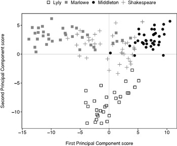
Figure 1.1 PCA scatterplot of 2,000-word non-overlapping segments of plays listed in Table 1.1, using the 500 most frequent words.
The first principal component (the x-axis) is the most important latent factor in the various correlations between the word-variables in the segments, and the second principal component (the y-axis) is the second most important (independent) latent factor. The relative distances between the points or ‘observations’ within this space represent degrees of affinity, so that segments of similar stylistic traits – specifically, similar rates of occurrence of our 500 words – cluster tightly together, whereas dissimilar segments are plotted further apart.
To make it easier to read the scatterplot, we use different symbols to label segments belonging to different authors. Although the separation between them is not perfect, segments belonging to the same author tend to cluster together, with Marlowe's segments (plotted as grey squares) typically scoring low on the first principal component and high on the second principal component. The PCA algorithm determines a weighting for each word, negative or positive, to give the best single combination to express the collective variability of all 138 segments’ word uses. Marlowe's low score for the first principal component means that the Marlowe segments relatively rarely use the words with a high positive weighting on this component and relatively frequently use the words with a high negative weighting. The algorithm then identifies a second set of weightings for the words, to best account for the remaining collective variability of the 138 segments’ word uses after the first principal component has accounted for its fraction of the collective variability. The Marlowe segments use the words with high positive weightings on this second principal component relatively often and the words with high negative ratings relatively rarely. We could, in theory, go on to calculate further principal components (a third, a fourth, and so on) until we run out of variance in the data – which must in any case happen for this experiment when we calculate the 500th principal component and so exhaust our 500 variables’ capacity to differ from one another. The most important consideration here is that this method demonstrably captures the affinity of segments by single authors, with Middleton's segments (plotted as black circles) typically scoring high on both axes. Lyly's segments cluster away from the others, scoring comparatively low on the second principal component, whereas Shakespeare's segments gravitate towards the centre of the scatterplot, forming a stylistic ‘bridge’ between the other authors.
We have plotted the first and second principal components – those which account for the greatest and second greatest proportion of the variance – and what emerge there are separations by author. This is evidence that authorship is a more important factor in stylistic differentiation than other groupings, such as genre or date, as we show below. However, there may be times when we may not be interested in the most important factors, whatever they may be. Since PCA can create as many components as there are variables, it is possible to target a particular factor. If we were interested in date, for example, we could work through the other components to find one which differentiates the sample by date – that is, which single set of weightings given to the 500 words will separate those favoured early in the period from those favoured late in the period – and then either use that component to classify a sample of unknown date, or explore the stylistics of the date-based groupings by examining the patterns of word-variables that create the component.
A different pattern in the data of the first two principal components emerges if we simply re-label the points on the scatterplot according to genre (Figure 1.2). The underlying data has not changed, only the labels of the points. Along the first principal component, segments appear to cluster in generic groups from ‘heroical romance’ (plotted as black circles) through to ‘history’ (grey plus symbols), ‘tragedy’ (unfilled triangles), and ‘comedy’ (unfilled squares). This perhaps explains some of the internal variation evident within the authorial clusters identified in Figure 1.1. For example, segments from Marlowe's ‘heroical romance’ plays, 1 and 2 Tamburlaine the Great, cluster tightly together, whereas segments from his Edward the Second are plotted closer to – sharing stylistic traits with – segments from Shakespeare's play of the same genre, Richard the Third. Similarly, Lyly's ‘comedy’ Mother Bombie is plotted higher on the second principal component than segments from his other ‘classical legend’ comedies.Footnote 13
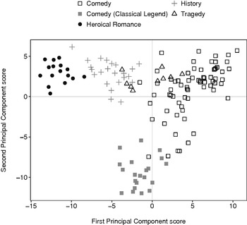
Figure 1.2 PCA scatterplot of 2,000-word non-overlapping segments of plays listed in Table 1.1, labelled by genre, using the 500 most frequent words.
PCA works by finding weightings for the variables to establish new composite variables – the components. We can examine these weightings to find out which variables contribute the most to a given component. To visualise the weightings, we can plot them in a separate biaxial chart, show them as a column or bar chart, or display them on the same chart as the segments in the form of a ‘biplot’. The biplot allows us to visualise the contributions of each word-variable in the same two-dimensional space as the play segments (Figure 1.3).Footnote 14 It shows the segment scores (as in Figures 1.1 and 1.2), but also overlays on these the weightings for the word-variables. In a biplot, the word-variables are generally represented by an arrow or ‘vector’ drawn from the origin – the point where the x and y axes intersect, i.e., 0,0 – rather than as points. This is a reminder that each variable is an axis, and the length and direction of the vector is also a convenient indication of the importance of that variable for a given component.
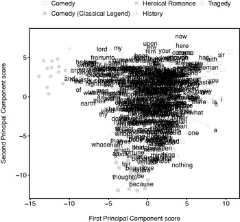
Figure 1.3 PCA biplot of 2,000-word non-overlapping segments of plays listed in Table 1.1, labelled by genre, using the 500 most frequent words.
The positions of the ends of the vectors in the biplot are determined by the weightings of the variables for the two components, re-scaled to fit into the chart space.Footnote 15 Since the vectors are scaled to fit the biplot, the distance between the end or ‘head’ of a vector and a play segment is unimportant; what matter are the directions and relative lengths of the vectors.
The direction of a vector indicates how a word-variable contributes to each of the principal components. A segment with many instances of the word-variables strongly positively weighted in one of the principal components will have been ‘driven’ in that direction, whereas a segment dominated by word-variables weak in both components will be plotted towards the origin.Footnote 16 The relative length of a vector corresponds to the magnitude of the contribution. In Figure 1.3, a long vector extending in an easterly direction shows that the corresponding word-variable has a heavy positive weighting on the first principal component, while a short vector extending in a southerly direction shows that the corresponding word-variable has a weak negative weighting on the second principal component.
If, as in Figure 1.3, all 500 of the word-variable vectors are drawn, the biplot becomes too difficult to analyse. Instead, we can redraw the biplot highlighting only word-variables of thematic interest or those belonging to a particular grammatical class. For example, Figure 1.4 gives the same biplot with only vectors for word-variables of personal pronouns drawn.
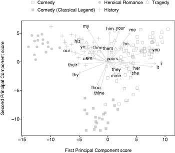
Figure 1.4 PCA biplot of 2,000-word non-overlapping segments of plays listed in Table 1.1, labelled by genre, using the 500 most frequent words and highlighting personal pronouns.
Inspection of the biplot reveals that ‘comedy’ segments plotted to the east of the origin are dominated by singular personal pronouns, such as the first-person I, me, and mine, the second-person formal you, your, and yours, and the third-person he, she, it, him, and her. By contrast, the ‘heroical romance’ and ‘history’ segments plotted west of the origin are dominated by plural personal nouns, such as the first-person we, us, and our, the second-person ye, and the third-person their, while ‘classical legend’ comedy segments, plotted south-west of the origin, favour the second-person informal singular thou and thine forms. Speeches in heroical romances, tragedies, and history plays are evidently cast more in terms of collectives, as we might expect with a focus on armies in battle and political factions. Comedies, on the other hand, tend to include more one-on-one interpersonal exchanges, so that the singular pronouns figure more strongly in their dialogue.
Random Forests
The decision-making process is often characterised as a series of questions: answers to one question may lead to a decision being reached, or prompt a further question – or series of questions – until a decision is made. For example, a doctor asks a patient to describe their symptoms and they respond that they have a runny nose. Among other conditions, rhinorrhea – the technical term for a runny nose – is a symptom common to both allergy (e.g. hayfever) and certain infections (e.g. the common cold). To reach a diagnosis, the doctor may ask further questions of the patient: how long have the symptoms persisted? Is the nasal discharge clear or coloured? Does the patient suffer from itchy eyes, aches, or fever?
While the common cold often causes a runny nose and may sometimes occasion aches, it rarely results in fever or itchy eyes and typically does not last longer than a fortnight. By contrast, rhinorrhea and itchy eyes are frequent allergic reactions and may last as long as the patient is in contact with the allergy trigger – minutes, hours, days, weeks, even months and seasons. (The term ‘hayfever’ is somewhat misleading, because fever and aches are not typical allergic responses.) Our hypothetical doctor's decision-making process may be visualised as a decision tree (Figure 1.5).
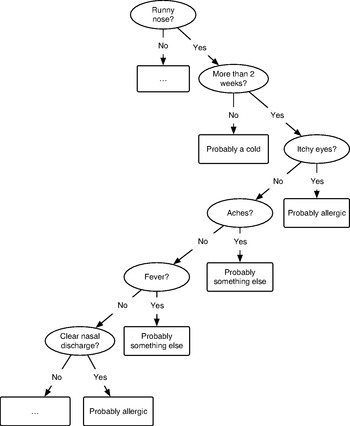
Figure 1.5 Binary decision tree diagram.
Of course, this is a simplified example (and correspondingly simple visualisation) of a complex consideration of multiple variables, some of which are ‘weighted’ – or more important to the decision-making process than others.
Random Forests is a supervised machine-learning procedure for classifying data using a large number of decision trees.Footnote 17 Whereas our hypothetical doctor relied upon centuries of accumulated knowledge to identify attributes or features distinguishing one medical condition from another, decision tree algorithms instead begin by testing variables in a set of data with a known shared attribute (a so-called ‘training set’) to derive a rule – like the series of questions posed by the doctor – that best performs the task of splitting the data into desired categories or classes. At each succeeding level of the tree, the sub-sets created by the splits are themselves split according to another rule, and the tree continues to grow in this fashion until all of the data has been classified. Once a decision tree is ‘trained’ to classify the data of the training set, it can then be employed to classify new, unseen data.Footnote 18
Random Forests combines the predictive power of hundreds of such decision trees (hence ‘forests’). Each tree is derived using a different and random sub-set of the training dataset and variables. To enable validation of the technique and to avoid the problem of ‘over-fitting’,Footnote 19 randomly selected segments of the training set are withheld from the algorithm so that they do not inform the construction of the decision trees (and thus allowing us to determine how accurate the trees’ predictions are in classifying these withheld segments). By default, one-third of all training-set segments are withheld for this purpose. This testing, using segments of a known class or category, treated as if this was unknown, gives us an expected error rate for when the decision trees are used to classify new data. The higher the classification error rate, the weaker the relationship between the variables and the classes, and vice versa. Hundreds of such trees are constructed, and for each classification to be made each tree contributes one vote to the outcome. This aggregation of decision trees evens out any errors made by individual trees that may arise from the construction of apparently reliable – but in fact false – rules based on anomalous data.Footnote 20
By way of example, we use Intelligent Archive to generate word-frequency counts for the 500 most frequent words across the selection of plays listed in Table 1.1, segmented into 2,000-word non-overlapping blocks and discarding any smaller blocks that remain. As before, proper nouns, foreign-language passages, and stage directions are excluded from the procedure. This produces a large table of 138 rows and 500 columns, which we split into two separate tables: one to serve as our training dataset (109 rows, 500 columns), and another containing all of the segments from each author's first-listed play to serve as a test dataset (29 rows, 500 columns). After a randomly selected one-third of segments in the training dataset are withheld by the algorithm to be tested later, 500 decision trees are populated using the remaining two-thirds of the training dataset, trying 22 random word-variables at each ‘split’ in the decision tree.Footnote 21 A diagram of one of the decision trees populated in this experiment is given in Figure 1.6, in which the rules are expressed as the rates of occurrence of a word-variable per 2,000 words. Thus, according to its rules, if a 2,000-word segment contains 1 or fewer instances of the word hath and 61 or fewer instances of the word and, then this decision tree predicts it is a Middleton segment.Footnote 22 Of course, as the outcome of a single decision tree, this prediction would count as one out of 500 votes cast by the ‘forest’ of trees.
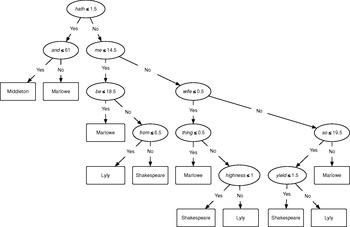
Figure 1.6 Diagram of a single binary decision tree populated for Random Forests classification of 2,000-word non-overlapping segments in a training dataset of 109 segments drawn from plays listed in Table 1.1, using the 500 most frequent words.
The algorithm then uses the decision trees to classify the training dataset as a whole, with the randomly withheld one-third of segments reintroduced. This produces an expected error rate for when the unseen test dataset will be classified later. Table 1.2 gives the confusion matrix for the 109 segments of the entire training dataset, tabling four misclassifications made by the decision trees: three segments of The Jew of Malta assigned to Shakespeare, and one segment of Richard the Third assigned to Marlowe. This produces a promisingly low expected error rate of 3.67 per cent (= 4 ÷ 109 × 100).
Table 1.2 Confusion matrix for Random Forests classification of 2,000-word non-overlapping segments in a training dataset of 109 segments drawn from plays listed in Table 1.1, using the 500 most frequent words
| Lyly, John | Marlowe, Christopher | Middleton, Thomas | Shakespeare, William | Misclassification (%) | |
|---|---|---|---|---|---|
| Lyly, John | 23 | 0 | 0 | 0 | 0 |
| Marlowe, Christopher | 0 | 24 | 0 | 3 | 11 |
| Middleton, Thomas | 0 | 0 | 28 | 0 | 0 |
| Shakespeare, William | 0 | 1 | 0 | 30 | 3 |
The decision trees are then used to classify all of the data – i.e., the whole training dataset, including the previously withheld segments, as well as the newly introduced segments of the test dataset. Table 1.3 gives the resulting confusion matrix. The decision trees classify all of the segments in the test dataset correctly, resulting in a classification error rate of 2.89 per cent for all of the segments in both the training and test datasets – that is, 4 misclassified segments out of the total 138.
Table 1.3 Confusion matrix for Random Forests classification of 109 training and 29 test segments of plays listed in Table 1.1, segmented into 2,000-word non-overlapping blocks, using the 500 most frequent words
| Lyly, John | Marlowe, Christopher | Middleton, Thomas | Shakespeare, William | Misclassification (%) | |
|---|---|---|---|---|---|
| Lyly, John | 29 | 0 | 0 | 0 | 0 |
| Marlowe, Christopher | 0 | 32 | 0 | 3 | 8 |
| Middleton, Thomas | 0 | 0 | 36 | 0 | 0 |
| Shakespeare, William | 0 | 1 | 0 | 37 | 2 |
Delta
Delta is a supervised method introduced by John Burrows to establish the stylistic difference between two or more texts by comparing the relative frequencies of very common words.Footnote 23 Although well established as a tool for authorship attribution study, Delta is also used more broadly as a means to describe ‘the relation between a text and other texts in the context of the entire group of texts’.Footnote 24
In its usual deployment, the procedure establishes a series of distances between a single text of interest and a comparison set typically comprising a series of authorial sub-sets of texts. The author with the lowest distance score is judged to be the ‘least unlikely’ author of the mystery text.Footnote 25 There are two main steps. The procedure begins by generating counts of high-frequency words in the ‘test’ text and comparison set. Counts for individual texts in the comparison set are retained, allowing Delta to derive both a mean figure for the set as a whole, and a standard deviation – a measure of the variation from that mean – for each variable.Footnote 26 The counts on the chosen variables – usually very common words – are transformed into percentages to account for differing sizes of text and then into z-scores by taking the difference between the word counts and the mean of the overall set and dividing that by the standard deviation for the variable. Using z-scores has the advantage that low-scoring variables are given equal weight with high-scoring ones, since a z-score is the number of standard deviations of an observation from the mean, unrelated to the size of the original units. The z-score also takes into account the amplitude of fluctuations within the counts. Wide fluctuations result in a high standard deviation and thus a lower z-score.
The differences between z-scores for the test text and each authorial sub-set are then found for each variable, adding up the absolute differences – that is, ignoring whether the figures are positive or negative – to form a composite measure of difference (or ‘Delta’ distance). The procedure is complete at this point, with a measure for the overall difference between the test text and each of the authorial sub-sets within the comparison set.
To illustrate the method, consider an example using the set of sixteen plays listed in Table 1.1, with four plays each by Lyly, Marlowe, Middleton, and Shakespeare. We first generate frequency counts for the 100 most common function words in all 16 plays and transform these into percentages. We then choose one Lyly play at random to serve as a test text – in this case, Galatea – and withdraw this play from the Lyly authorial sub-set. We transform the word-frequency scores for Galatea into z-scores, using the means and standard deviations for the whole set of sixteen plays. We do the same for the mean scores for the Lyly, Marlowe, Middleton, and Shakespeare plays – the Lyly set consisting of the three remaining plays, the others retaining their full sub-set of four plays each. To arrive at a composite distance measure, we add up the absolute differences between the Galatea z-scores and each of the authorial sub-set z-scores for the 100 word-variables. Figure 1.7 shows the resulting Delta distances as a column chart.
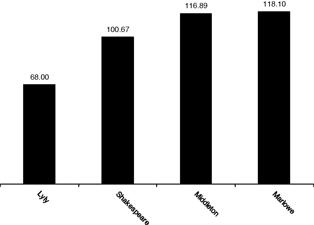
Figure 1.7 Delta distances between Galatea and four authorial sub-sets.
When treated as a mystery text, Galatea finds its closest match in a Lyly sub-set based on the three remaining Lyly plays, with a Delta distance of 68. Shakespeare, with a Delta distance of 100.67, is the next nearest author, followed by Middleton (116.89) and Marlowe (118.10). We can then do the same for the other three Lyly plays, withdrawing each in turn and testing the resemblance between that play and each of the four authorial sub-sets. As it turns out, and as we would expect (but could not guarantee), each Lyly play matched the sub-set of remaining Lyly plays most closely.
We repeat the procedure for the other authors along the same lines, holding out and testing each play in turn. In every case, the known author was the closest match, with the exception of The Jew of Malta (Figure 1.8), which matched Shakespeare most closely (with a Delta distance of 68.08), then Middleton (at 83.65), then Lyly (at 86.22) – with Marlowe the most distant at 112.22.Footnote 27
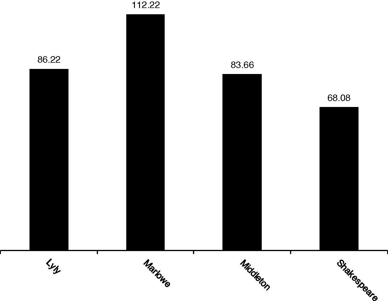
Figure 1.8 Delta distances for The Jew of Malta and four authorial sub-sets.
Evidently, this play represents a radical departure from Marlowe's typical practice in the use of very common function words (established on the basis of the three other plays in the sub-set). As the only (potentially) incorrect attribution out of sixteen Delta tests, this anomalous result is certainly worthy of further investigation. However, for the purposes of demonstration, it is enough to note that, overall, Delta is a good – but perhaps not infallible – guide to authorship and stylistic difference, even when using small sub-sets to represent an author.
Shannon Entropy
Shannon entropy is a measure of the repetitiveness of a set of data, and is the key concept in information theory as developed by Claude Shannon in the 1940s.Footnote 28 Shannon entropy calculates the greatest possible compression of the information provided by a set of items considered as members of distinct classes. A large entropy value indicates that the items fall into a large number of classes, and thus must be represented by listing the counts of a large number of these classes. In an ecosystem, this would correspond to the presence of a large number of species each with relatively few members. The maximum entropy value occurs where each item represents a distinct class. Minimum entropy occurs where all items belong to a single class. In terms of language, word tokens are the items and word types the classes.Footnote 29 A high-entropy text contains a large number of word types, many with a single token. A good example would be a technical manual for a complex machine which specifies numerous distinct small parts. A low-entropy text contains few word types, each with many occurrences, such as a legal document where terms are repeated in each clause to avoid ambiguity. Entropy is a measure of a sparse and diverse distribution versus a dense and concentrated one. High-entropy texts are demanding of the reader and dense in information – they constantly move to new mental territories; they are taxing and impressive. Low-entropy texts are reassuring and familiar – they are implicit in their signification, assuming common knowledge, while high-entropy texts specify and create contexts for themselves. High-entropy texts contain more description and narrative, while low-entropy texts contain more dialogue.
Shannon entropy is defined as the negative of the sum of the proportional counts of the variables in a dataset each multiplied by its logarithm.Footnote 30 A line consisting of a single word-type repeated five times (e.g. ‘Never, never, never, never, never!’ King Lear 5.3.307) has a single variable with a proportion of  (or 1). The log of 1 is 0. The Shannon entropy of the line is therefore:
The line ‘Tomorrow, and tomorrow, and tomorrow’ from Macbeth (5.5.18) has three instances of tomorrow and two of and. The proportional count for tomorrow is  (or 0.6) and for and is
  (or 0.4), thus the Shannon entropy for the line is
For a final comparison, consider the line: ‘If music be the food of love, play on’ (Twelfth Night 1.1.1). This time, each of the nine words making up the line occurs only once. Since each word-variable has a proportional score of  (or ≈ 0.111), the Shannon entropy for this line is:
– a higher score than for our two previous examples, reflecting comparatively greater variability in word use.Footnote 31
t-tests
Consider the following experiment. We compile a set of Shakespeare's comedies (All's Well That Ends Well, As You Like It, The Merchant of Venice, A Midsummer Night's Dream, Much Ado About Nothing, and Twelfth Night) and a set of Shakespeare's tragedies (Antony and Cleopatra, Hamlet, King Lear, Othello, Romeo and Juliet, and Troilus and Cressida). Are there more instances, on average, of the word death in the tragedies compared with the comedies? If there is a difference in these averages, how consistent is it, in the sense that any large group of tragedies will have more occurrences of death overall? Our experiment calls for us to find a way to see past mere averages to the varying counts that lie behind them.
The occurrence of death in each of these plays, expressed as a percentage of the total number of words, is 0.08, 0.03, 0.05, 0.08, 0.08, and 0.05 respectively for the comedies, and 0.14, 0.13, 0.08, 0.06, 0.29, and 0.06 for the tragedies. The mean for the comedies is 0.062, and for the tragedies it is 0.127 – more than twice as large. But how can we take the fluctuations within the groups into account?
One way to do this is to use a t-test, a common statistical procedure to determine whether the ‘mean’ or average of a ‘population’ – that is, all members of a defined group or dataset from which a selection or ‘sample’ is drawn – differs significantly from a hypothetical mean or the mean of another population. The test was first proposed in 1908 by W. S. Gosset, writing under the pseudonym ‘Student’ while working in quality control for the Guinness brewery in Ireland.Footnote 32 Student's t-test, as it has come to be known, generates a simple metric called the t-value, calculated as the difference in means between two sets divided by the combination of their standard deviations. A high t-test score means that the average use in one set is much higher or lower than the use in a second set, and the word overall does not fluctuate much.
Student's t-test assumes that the two populations under investigation follow a ‘normal distribution’ and have an equal variance (i.e., the data in both populations is ‘spread’ or ‘scattered’ equally).Footnote 33 In 1947 B. L. Welch adapted Student's t-test to accommodate populations of unequal variance,Footnote 34 and we use this variation in the present experiment and generally throughout this book. For Welch's t-test, the one we have used in this book, the formula is:
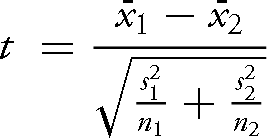
Here  and
and  are the means of the first and second samples,
  and
and  the squared standard deviations of the first and second samples, and n1 and n2 the number of items in each respective sample. For our experiment, we already have the means (as above, 0.062 and 0.127), and the standard deviations are 0.021 and 0.087 for the comedies and tragedies respectively. The sample size is 6 for both sets. Using these figures, the formula produces a t-value of –1.778.
The other necessary piece of information is the number of degrees of freedom in the analysis. The more degrees of freedom, the more information the result is based on and the more confident we can be that the result reflects an underlying truth. Degrees of freedom in the t-test depend on the number of samples, but with Welch's t-test we are allowing for the possibility of different variances for the two groups, and estimating the true number of degrees of freedom requires taking into account the distribution of the data using the Welch-Satterthwaite formula.Footnote 35
The result in this case is 5.6. Given this number, we can find a t-test probability by consulting a table or using a t-test probability calculator.Footnote 36 This t-test probability (or ‘p-value’) indicates how often a difference like this would come about merely by chance, even when the two sets in fact belong to the same overall population, given the sample size. For this experiment, using a figure of 5.6 for the relevant degrees of freedom results in a p-value of 0.129. This is the probability (given that the data is normally distributed) that the two samples come from the same parent population – that the difference is a matter of local variation rather than something underlying and consistent. That is, 13 per cent of the time (one time in seven or eight) we should expect to see this apparent difference between the comedies and tragedies purely by chance alone, even if comedies and tragedies have no underlying preference for or against using the word death. This suggests that although the tragedies in our sample on average have twice the instances of the word, the fluctuations within the sets and the small number of samples mean that we should not base any broad conclusions on this result.
Glancing at the proportional scores for death in these texts might have indicated the same thing. There is one aberrant high score, for Romeo and Juliet, which accounts for a great deal of the high average for the set of tragedies overall, and there are three comedies at 0.8, which are all higher than the two lowest-scoring tragedies at 0.6. The t-test offers a way to treat these fluctuations systematically, a summary statistic which can be carried over from one comparison to another, and a broad indication about the inferences we can safely make about wider populations (such as about Shakespeare comedy and tragedy in general) from the current sample.
PCA, Random Forests, Delta, Shannon entropy, and the t-test are all well-established tools that we have found useful in making sense of the abundant, multi-layered data which can be retrieved from literary texts. They take us beyond what we can readily see with the naked eye, as it were – a count that stands out as high or low, or an obvious pattern of association between variables or samples – to larger-scale, more precise summaries that have some in-built protections from bias. PCA is a data reduction method; Random Forests a classification tool; Delta a distance measure; Shannon entropy a density metric; and the t-test takes us back to single variables and the question of whether two sets of counts have an underlying difference, or only an apparent one. They are just five of the numerous methods available, and by no means the most complex, but they are all tried and tested and offer a useful range. They come from different eras and were developed for different purposes – only Delta was devised specifically for computational stylistics. All five can be used both to test a hypothesis and to explore data more inductively, as we demonstrate in the chapters that follow.


