


1. Introduction
Flows that are driven by buoyancy forces are a common occurrence in nature as well as in technological applications. The driving mechanism is the temperature dependence of the fluid density, which leads to density variations when heat is transported through the fluid. A simplified paradigm for such flows is Rayleigh–Bénard convection (RBC), which consists of a fluid layer that is heated from below and cooled from above (Chandrasekhar Reference Chandrasekhar1981). While the understanding of RBC has increased substantially in the past decades (see, for example, Ahlers, Grossmann & Lohse Reference Ahlers, Grossmann and Lohse2009; Chillà & Schumacher Reference Chillà and Schumacher2012; Verma Reference Verma2018), it must be noted that a multitude of additional forces, such as those generated by rotation and magnetic fields, can affect buoyancy-driven convection in nature or in industrial applications. The effects of these forces have been relatively less explored. The present study deals with magnetoconvection, that is, thermal convection of electrically conducting fluids under the effect of magnetic fields.
In magnetoconvection, flows are acted upon by buoyancy as well as by Lorentz forces generated due to a magnetic field (Weiss & Proctor Reference Weiss and Proctor2014). Convection in the Sun and planetary dynamos are examples of magnetoconvection occurring in nature where the magnetic field is maintained by the flow. In technological applications, the magnetic field is usually not caused primarily by the flow but is imposed externally. Examples are liquid metal batteries for renewable energy storage, growth of semiconductor monocrystals, flow control of hot metal melts by electromagnetic brakes in metallurgy, and heat transfer in blankets in nuclear fusion reactors.
Magnetoconvection is governed by the equations for conservation of mass, momentum and energy as well as Maxwell's equations and Ohm's law. The governing non-dimensional parameters of magnetoconvection are (i) the Rayleigh number  ${{Ra}}$, the ratio of buoyancy to dissipative forces, (ii) the Prandtl number
  ${{Pr}}$, the ratio of kinematic viscosity to thermal diffusivity, (iii) the Hartmann number
  ${{Ha}}$, the ratio of Lorentz to viscous forces, and (iv) the magnetic Prandtl number
  ${{Pm}}$, the ratio of kinematic viscosity to magnetic diffusivity. Instead of the Hartmann number, the free-fall interaction parameter
  $N_f = {{Ha}}^2 \sqrt {{{Pr}}/{{Ra}}}$, also called the Stuart number, can be used as a governing parameter (Liu, Krasnov & Schumacher Reference Liu, Krasnov and Schumacher2018; Zürner et al. Reference Zürner, Schindler, Vogt, Eckert and Schumacher2020; Xu, Horn & Aurnou Reference Xu, Horn and Aurnou2022). The free-fall interaction parameter represents the ratio of magnetic and buoyant forcing in the fluid. The important non-dimensional output parameters of magnetoconvection are (i) the Nusselt number
  ${{Nu}}$, which quantifies the global heat transport, (ii) the Reynolds number
  ${{Re}}$, the ratio of inertial forces to viscous forces, and (iii) the magnetic Reynolds number
  ${{Rm}}$, the ratio of induction to diffusion of the magnetic field. For sufficiently small magnetic Reynolds numbers, the induced magnetic field is negligible compared to the applied magnetic field and is therefore neglected in the expressions of Lorentz force and Ohm's law (Roberts Reference Roberts1967; Davidson Reference Davidson2017; Verma Reference Verma2017, Reference Verma2019). In such cases, referred to as quasi-static magnetoconvection, the induced magnetic field adjusts instantaneously to the changes in velocity. In the quasi-static approximation, there exists a one-way influence of the magnetic field on the flow only.
Magnetoconvection has been studied theoretically in the past (e.g. Chandrasekhar Reference Chandrasekhar1981; Houchens, Witkowski & Walker Reference Houchens, Witkowski and Walker2002; Busse Reference Busse2008) as well as with the help of experiments (e.g. Nakagawa Reference Nakagawa1957; Fauve, Laroche & Libchaber Reference Fauve, Laroche and Libchaber1981; Cioni, Chaumat & Sommeria Reference Cioni, Chaumat and Sommeria2000; Aurnou & Olson Reference Aurnou and Olson2001; Burr & Müller Reference Burr and Müller2001; King & Aurnou Reference King and Aurnou2015; Vogt et al. Reference Vogt, Ishimi, Yanagisawa, Tasaka, Sakuraba and Eckert2018, Reference Vogt, Yang, Schindler and Eckert2021; Zürner et al. Reference Zürner, Schindler, Vogt, Eckert and Schumacher2020; Grannan et al. Reference Grannan, Cheng, Aggarwal, Hawkins, Xu, Horn, Sánchez- Álvarez and Aurnou2022) and numerical simulations (e.g. Liu et al. Reference Liu, Krasnov and Schumacher2018; Yan et al. Reference Yan, Calkins, Maffei, Julien, Tobias and Marti2019; Akhmedagaev et al. Reference Akhmedagaev, Zikanov, Krasnov and Schumacher2020a,Reference Akhmedagaev, Zikanov, Krasnov and Schumacherb; Nicoski, Yan & Calkins Reference Nicoski, Yan and Calkins2022). A horizontal magnetic field has been found to cause the large-scale rolls to become quasi-two-dimensional and align in the direction of the field (Fauve et al. Reference Fauve, Laroche and Libchaber1981; Busse & Clever Reference Busse and Clever1983; Burr & Müller Reference Burr and Müller2002; Yanagisawa et al. Reference Yanagisawa, Hamano, Miyagoshi, Yamagishi, Tasaka and Takeda2013; Tasaka et al. Reference Tasaka, Igaki, Yanagisawa, Vogt, Zürner and Eckert2016; Vogt et al. Reference Vogt, Ishimi, Yanagisawa, Tasaka, Sakuraba and Eckert2018, Reference Vogt, Yang, Schindler and Eckert2021). These self-organized flow structures reach an optimal state characterized by a significant increase in heat transport and convective velocities (Vogt et al. Reference Vogt, Yang, Schindler and Eckert2021). In contrast, strong vertical magnetic fields suppress convection (Chandrasekhar Reference Chandrasekhar1981; Cioni et al. Reference Cioni, Chaumat and Sommeria2000; Akhmedagaev et al. Reference Akhmedagaev, Zikanov, Krasnov and Schumacher2020a,Reference Akhmedagaev, Zikanov, Krasnov and Schumacherb; Zürner et al. Reference Zürner, Schindler, Vogt, Eckert and Schumacher2020), with the flow ceasing above a critical Hartmann number. At this threshold, the flow in the centre is fully suppressed with convective motion only in the vicinity of sidewalls (Busse Reference Busse2008; Liu et al. Reference Liu, Krasnov and Schumacher2018; Akhmedagaev et al. Reference Akhmedagaev, Zikanov, Krasnov and Schumacher2020a,Reference Akhmedagaev, Zikanov, Krasnov and Schumacherb; Zürner et al. Reference Zürner, Schindler, Vogt, Eckert and Schumacher2020) if they exist. These so-called wall modes, which are also present in confined rotating convection (Zhong, Ecke & Steinberg Reference Zhong, Ecke and Steinberg1991; Ecke, Zhong & Knobloch Reference Ecke, Zhong and Knobloch1992; Goldstein et al. Reference Goldstein, Knobloch, Mercader and Net1993, Reference Goldstein, Knobloch, Mercader and Net1994; Liu & Ecke Reference Liu and Ecke1999; King, Stellmach & Aurnou Reference King, Stellmach and Aurnou2012), are particularly relevant in technical applications in closed vessels. Hurlburt, Matthews & Proctor (Reference Hurlburt, Matthews and Proctor1996) and Nicoski et al. (Reference Nicoski, Yan and Calkins2022) studied convection with tilted magnetic fields. The results of Hurlburt et al. (Reference Hurlburt, Matthews and Proctor1996) suggest that the mean flows tend to travel in the direction of the tilt. Nicoski et al. (Reference Nicoski, Yan and Calkins2022) reported qualitative similarities between convection with a tilted magnetic field and that with a vertical magnetic field in terms of the behaviour of convection patterns, heat transport and flow speed.
It must be noted that all the aforementioned works on magnetoconvection have been restricted to a uniformly imposed magnetic field, which is an idealized approximation. However, in engineering applications such liquid metal batteries (Kelley & Weier Reference Kelley and Weier2018), cooling blankets in fusion reactors (Mistralengo et al. Reference Mistralengo, Bühler, Smolentsev, Klüber, Maione and Aubert2021), electromagnetic stirring (Davidson Reference Davidson1999), electromagnetic brakes (Davidson Reference Davidson2017) and non-contact flow measurements involving Lorentz force velocimetry (Thess, Votyakov & Kolesnikov Reference Thess, Votyakov and Kolesnikov2006), the imposed magnetic fields are localized and thus vary in space. Further, strong homogeneous fields in large regions of space can be generated only by magnets of large size, which are difficult to design and very costly to build and operate (Barleon, Mack & Stieglitz Reference Barleon, Mack and Stieglitz1996). Thus it is important to understand the impact of spatially varying magnetic fields on magnetohydrodynamic flows. Although there are several studies on the channel flow of liquid metals under the influence of non-homogeneous magnetic fields (see, for example, Sterl Reference Sterl1990; Votyakov & Kassinos Reference Votyakov and Kassinos2009; Moreau, Smolentsev & Cuevas Reference Moreau, Smolentsev and Cuevas2010; Albets-Chico et al. Reference Albets-Chico, Grigoriadis, Votyakov and Kassinos2013; Klüber, Bühler & Mistrangelo Reference Klüber, Bühler and Mistrangelo2020), no similar work on magnetoconvection has been conducted so far, to the best of our knowledge.
Convection flows in horizontally extended domains are often organized into prominent and coherent large-scale patterns that persist for very long times and can extend over scales in the lateral direction that are much larger than the domain height. These so-called superstructures have a strong influence on the turbulent transport properties of the flow. A prominent example of such superstructures is the granulation at the surface of the Sun (Schumacher & Sreenivasan Reference Schumacher and Sreenivasan2020). While the understanding of the process of formation and evolution of these superstructures and their characteristic scales in the absence of magnetic fields has improved significantly over recent years (see, for example, Pandey, Scheel & Schumacher Reference Pandey, Scheel and Schumacher2018; Stevens et al. Reference Stevens, Blass, Zhu, Verzicco and Lohse2018; Krug, Lohse & Stevens Reference Krug, Lohse and Stevens2020), the case with inhomogeneous magnetic fields still leaves several questions open as the physical complexity is increased.
In the present work, we attempt to fill some of these gaps and study the effect of strong spatially varying magnetic fields in turbulent convection under the quasi-static approximation. The effects of localized magnetic fields on turbulent superstructures and their impact on the local and global turbulent heat and momentum transport are explored. We consider a Rayleigh–Bénard cell with fringing magnetic fields generated by semi-infinite magnetic poles. The strength of the magnets is such that convection in the regions of strong magnetic fields is fully suppressed in the bulk. Thus in a single convection cell, we obtain different local regimes of magnetoconvection, ranging from the turbulent regime in the regions of weak magnetic flux to wall-attached convection in the regions of strong magnetic flux. As mentioned earlier, the superstructures are formed in horizontally extended domains, hence the convection cell employed in our present study has a large aspect ratio. We study the spatial variation of size and orientation of turbulent superstructures along with the turbulent transport inside the convection cell. We also study wall-attached convection in the regions of strong magnetic flux regions, the wall modes. Although the set-up is a simple way to study the influence of spatially varying magnetic fields on convection, it permits us to carry out such a parametric study systematically. This is the main motivation of the present work. Future studies can be conducted in a similar manner for more complex arrangements.
The outline of the paper is as follows. Section 2 describes the magnetoconvection set-up along with the governing equations of magnetoconvection and the spatial distribution of the magnetic field. The details of our numerical simulations are also discussed in § 2. In § 3, we present the numerical results, detailing the behaviour of large-scale structures, the spatial distribution of heat and momentum transport along with their variations with the magnetic field, the dependence of the global heat and momentum transport on the fringe width, and wall-attached convection. We conclude in § 4 with a summary and an outlook.
2. Numerical model
2.1. Problem set-up and equations
We consider a horizontally extended convection cell of size  $l_x \times l_y \times H$ that is under the influence of a magnetic field generated by two semi-infinite permanent magnets. The north pole of one magnet faces the bottom of the convection cell, and the south pole of the second magnet faces the top of the convection cell. These magnets extend from
  $-\infty$ to
  $\infty$ in the
  $x$-direction, from
  $l_y/2$ to
  $\infty$ in the
  $y$-direction, from near the top wall to
  $\infty$ in the positive
  $z$-direction, and from near the bottom wall to
  $- \infty$ in the negative
  $z$-direction. A schematic of a vertical section of the arrangement is provided in figure 1(a). Using the model of Votyakov, Kassinos & Albets-Chico (Reference Votyakov, Kassinos and Albets-Chico2009) for permanent magnets, we obtain the following relations for the non-dimensional imposed magnetic field
  $\boldsymbol {B}_0=\{B_x, B_y, B_z \}$ generated in the above configuration:
 \begin{gather} B_x = 0, \end{gather}
 \begin{gather}B_y ={-}{\frac{1}{4{\rm \pi}}\,B_{z,max}}\ln \left[ \frac{(y - y_c)^2 - \{(z - z_c) - (H/2 + \delta)\}^2}{(y - y_c)^2 + \{(z - z_c) + (H/2+\delta)\}^2} \right], \end{gather}
 \begin{gather}B_z ={-}{\frac{1}{2{\rm \pi}}\,B_{z,max}} \arctan \left [\frac{2(H/2 + \delta)(y-y_c)}{(y-y_c)^2 + (z-z_c)^2 - (H/2+\delta)^2} \right ], \end{gather}
where  $y_c$ and
  $z_c$ are the
  $y$- and
  $z$-coordinates, respectively, of the cell-centre,
  $B_{z,max}$ is the maximum limiting value of the vertical component of the magnetic field at
  $y \rightarrow \infty$, and
  $\delta$ is the gap between the permanent magnet and the top/bottom wall (see figure 1). The aforementioned magnetic field distribution satisfies
  $\boldsymbol {\nabla }\times {\boldsymbol B}_0=0$ and
  $\boldsymbol {\nabla }\boldsymbol {\cdot } {\boldsymbol B}_0=0$. In the above configuration, the magnetic field is almost absent in nearly half of the RBC cell (for
  $y \lesssim l_y/2$), increases steeply about the midplane (
 $y \approx l_y/2$), and then becomes strong in the other half of the cell (for
  $y \gtrsim l_y/2$). A three-dimensional view of the convection cell used in our study with the density contours of the vertical component of the imposed magnetic field is shown in figure 1(b). The region where the gradient of the magnetic field is large is called the fringe zone; we provide a mathematical definition of the fringe zone later in this subsection. Henceforth, the region of the convection cell that is outside the gap between the magnets will be referred to as the weak magnetic flux region, and the one inside the gap will be referred to as the strong magnetic flux region.

Figure 1. (a) Schematic of the vertical section at  $x = x_c = l_x/2$ of the proposed magnetoconvection arrangement. The semi-infinite permanent magnets (in grey) generate the localized magnetic field represented by the vector plots drawn in the convection cell. The magnetic field distribution is described by (2.1)–(2.3). (b) A three-dimensional view of the convection cell used in our study, with the density contours of the vertical component of the normalized imposed magnetic field for
  $\delta /H=0.01$. Here,
  $O$ refers to the point at the origin, and
  $\delta$ is the gap between the magnetic pole and the convection cell.
Equations (2.2) and (2.3) imply that the spatial distribution of the magnetic field is strongly dependent on the gap width ( $\delta$) between the magnetic poles and the convection cell. In figures 2(a) and 2(b), we plot, respectively, the profiles of the normalized mean vertical magnetic field,
  $\langle B_z/B_{z,max} \rangle _{x,z}$, and the normalized mean horizontal magnetic field,
  $\langle |B_y|/B_{z,max} \rangle _{x,z}$, versus the normalized lengthwise coordinate
  $y/H$. In the above,
  $|{\cdot }|$ and
  $\langle {\cdot } \rangle _{x,z}$, respectively, represent the absolute value and averaging over
  $x$ and
  $z$. As is evident in figure 2(a), the gradient of the vertical magnetic field decreases as
  $\delta$ is increased. In the present set-up, we define the fringe zone as the region in which
  $0.1 < \hat {B}_z < 0.9$, where
 \begin{equation} \hat{B}_z = \frac{\langle B_z \rangle_{x,z} - B_{z,min,D}}{B_{z,max,D} - B_{z,min,D}}. \end{equation}
In the above,  $B_{z,max,D}$ and
  $B_{z,min,D}$ are, respectively, the maximum and minimum values of the vertical magnetic field in the convection cell. (It must be noted that
  $B_{z,max,D} \neq B _{z,max}$;
  $B_{z,max,D}$ is the maximum value of
  $B_z$ inside the convection cell, and
  $B_{z,max}$ is the maximum limiting value of
  $B_z$ at
  $y \rightarrow \infty$.) In figures 2(a,b), the curves describing the magnetic field profiles are represented as dashed lines in the fringe zone and as solid lines outside the fringe zone. The figures clearly show that the width of the fringe zone increases with an increase in
  $\delta$. Further, the horizontal component of the magnetic field on the lateral vertical midplane at
  $y=l_y/2$ increases with a decrease in
  $\delta$. These variations in the magnetic field profile affect the convection patterns along with the associated global heat transport, and will be studied in detail in the later sections.

Figure 2. Distribution of the profiles of (a) vertical magnetic field and (b) absolute value of the horizontal magnetic field, both averaged over  $x$ and
  $z$, along the lengthwise direction (normalized by the height
  $H$ of the cell) for different values of the normalized gap (
 $\delta ' = \delta /H$) between the magnetic poles and the thermal plates. The magnetic fields are normalized by the maximum value of the vertical magnetic field (
 $B_z'=B_z/B_{z,max}$ and
  $B_y'=B_y/B_{z,max}$). The curves are represented as dashed lines in the fringe zone, and as solid lines outside the fringe zone.
The study will be conducted under the quasi-static approximation, in which the induced magnetic field is neglected as it is very small compared to the applied magnetic field. This approximation is fairly accurate for magnetoconvection in liquid metals (Davidson Reference Davidson2017). The non-dimensionalized governing equations are
 \begin{gather} \boldsymbol{\nabla} \boldsymbol{\cdot} \boldsymbol{u}=0, \end{gather}
 \begin{gather}\frac{\partial \boldsymbol{u}}{\partial t} + \boldsymbol{u}\boldsymbol{\cdot} \boldsymbol{\nabla} \boldsymbol{u} ={-}\boldsymbol{\nabla} p + T\hat{z}+ \sqrt{\frac{{{Pr}}}{{{Ra}}}}\,\nabla^2 \boldsymbol{u}+ {{Ha}}_{z,max}^2\,\sqrt{\frac{{{Pr}}}{{{Ra}}}}\,(\,\boldsymbol{j} \times \tilde{\boldsymbol{B}}), \end{gather}
 \begin{gather}\frac{\partial T}{\partial t} + \boldsymbol{u} \boldsymbol{\cdot} \boldsymbol{\nabla} T = \frac{1}{\sqrt{{{Ra}}\,{{Pr}}}}\,\nabla^2 T, \end{gather}
 \begin{gather}\boldsymbol{j} ={-}\boldsymbol{\nabla} \phi + (\boldsymbol{u} \times \tilde{\boldsymbol{B}}), \end{gather}
 \begin{gather}\nabla^2 \phi = \boldsymbol{\nabla} \boldsymbol{\cdot} (\boldsymbol{u} \times \tilde{\boldsymbol{B}}), \end{gather}
where  $\boldsymbol {u}$,
  $\boldsymbol {j}$,
  $p$,
$p$,  $T$ and
  $\phi$ are the fields of velocity, current density, pressure, temperature and electrical potential, respectively, and
  $\tilde {\boldsymbol {B}}$ is the applied magnetic field normalized by
  $B_{z,max}$. The governing equations are made dimensionless by using the cell height
  $H$, the imposed temperature difference
  $\varDelta$, and the free-fall velocity
  $U = \sqrt {\alpha g\,\Delta H}$ (where
  $g$ and
  $\alpha$ are, respectively, the gravitational acceleration and the volumetric coefficient of thermal expansion of the fluid). The non-dimensional governing parameters are the Rayleigh number (
 ${{Ra}}$), the Prandtl number (
 ${{Pr}}$), the Hartmann number (
 ${{Ha}}_{z,max}$) based on
  $B_{z,max}$, and the normalized gap (
 $\delta '$) between the thermal plates and the magnetic poles. These parameters are defined as follows:
 \begin{equation} {{Ra}} = \frac{\alpha g\,\Delta H^3}{\nu \kappa}, \quad {{Pr}}= \frac{\nu}{\kappa}, \quad {{Ha}}_{z,max} = B_{z,max} H\sqrt{\frac{\sigma}{\rho \nu}}, \quad {\delta' = \frac{\delta}{H}}, \end{equation}
where  $\nu$ is the kinematic viscosity,
  $\kappa$ is the thermal diffusivity,
  $\rho$ is the density, and
  $\sigma$ is the electrical conductivity of the fluid. For the sake of brevity, we henceforth omit the prime from
  $\delta '$. In the next subsection, we describe the simulation details.
2.2. Numerical method
We conduct direct numerical simulations of our magnetoconvection set-up described in § 2.1. The spatial distribution of the magnetic field is given by (2.1)–(2.3). We use a second-order finite difference code developed by Krasnov, Zikanov & Boeck (Reference Krasnov, Zikanov and Boeck2011) and Krasnov et al. (Reference Krasnov, Akhtari, Zikanov and Schumacher2023) to solve numerically (2.5)–(2.9). The Prandtl number  ${{Pr}}$ is chosen to be 0.021, which is the same as that of mercury. The Rayleigh number is fixed at
  ${{Ra}}=10^5$. For our chosen
  ${{Pr}}$, the aforementioned value of
  ${{Ra}}$ causes significant turbulence in the regions of weak magnetic flux. For
  ${{Ra}}=10^5$, the critical Hartmann number (above which the bulk convection is suppressed) computed using the linear stability analysis of Chandrasekhar (Reference Chandrasekhar1981) for a uniform vertical magnetic field is
 \begin{equation} {{Ha}}_{z,c}=88.7. \end{equation}
In order to include the wall-attached convection regime in our analysis, we choose the maximum Hartmann number to be  ${{Ha}}_{z,max} = 120$, which is slightly higher than the critical Hartmann number.
As mentioned in § 1, we intend to study the behaviour of turbulent superstructures in our present work. For our chosen values of  ${{Ra}}$ and
  ${{Pr}}$, the typical length scales of the superstructures are 3–4 times the height of the domain (Pandey et al. Reference Pandey, Scheel and Schumacher2018). Therefore, in order to obtain good statistics, we choose the horizontal extent of our domain to be around 5 times the expected length scale of the superstructures. Furthermore, in order to capture more effectively the variation of the superstructures and the global heat transport with magnetic field strength, it is preferred that the domain is elongated along the
  $y$-direction, that is, along the gradient of the magnetic field. Therefore, we choose the domain size to be
  $l_x \times l_y \times H = 16 \times 32 \times 1$.
We employ a grid resolution of  $4800 \times 9600 \times 300$ points. The mesh is non-uniform in the
  $z$-direction, with stronger clustering of the grid points near the top and bottom boundaries. The elliptic equations for pressure, electric potential and temperature are solved based on applying cosine transforms in the
  $x$- and
  $y$-directions, and using a tridiagonal solver in the
  $z$-direction. The diffusive term in the temperature transport equation is treated implicitly. The time discretization of the momentum equation uses the fully explicit Adams–Bashforth backward-differentiation method of second order (Peyret Reference Peyret2002). A constant time step size of
  $1 \times 10^{-4}$ free-fall time units was chosen for our simulations, which satisfied the Courant–Friedrichs–Lewy (CFL) condition for all runs.
All the walls are rigid and electrically insulated such that the electric current density  $\boldsymbol {j}$ forms closed field lines inside the cell. The top and bottom walls are held fixed at
  $T=-0.5$ and
  $T=0.5$, respectively, and the sidewalls are adiabatic with
  $\partial T/\partial \eta =0$ (where
  $\eta$ is the component normal to the sidewall). All the simulations are initialized with the linear conduction profile for temperature (which is a function of the
  $z$-coordinate only) and a random noise of amplitude
  $A=0.001$ along the
  $z$-direction for velocity. We run the simulations initially on a coarse grid of
  $480 \times 960 \times 30$ points for 100 free-fall time units in which they converge to a statistically steady state. Following this, we refine the mesh successively to the required resolution of
  $4800 \times 9600 \times 300$ grid points, and allow the simulations to converge after each refinement. Once the simulations reach the statistically steady state at the highest resolution, they are run for a further 20–21 free-fall time units, and a snapshot of the flow field is saved after every free-fall time unit.
Table 1 lists the important parameters of our simulation runs. In this table, we also report the turbulent momentum transfer quantified by the global Reynolds number ( ${{Re}}_{global}$) and the turbulent heat transport quantified by the global Nusselt number (
 ${{Nu}}_{global}$). These quantities are given by
 \begin{gather} {{Re}}_{global} = u_{rms}\sqrt{{{Ra}} / {{Pr}}}, \end{gather}
 \begin{gather}{{Nu}}_{global} = 1 + \sqrt{{{Ra}}\,{{Pr}}}\,\langle u_z T\rangle_{V,t_N}, \end{gather}
where  $\langle {\cdot } \rangle$ represents averaging,
  $u_{rms} = \sqrt {\langle u_x^2 + u_y^2 + u_z^2 \rangle _{V,t_N}}$ with
  $V$ being the volume of the convection cell, and
  $t_N$ (also reported in table 1) is the number of free-fall times run by the solver after attaining a statistically steady state.
Table 1. Parameters of the simulations: the gap ( $\delta$) between the magnetic poles and the conducting walls, the global Reynolds number (
 ${{Re}}_{global}$), the global Nusselt number (
 ${{Nu}}_{global}$), and the number of free-fall time units (
 $t_N$) run by the solver after attaining statistically steady state. Here,
  ${{Re}}_{global}$ and
  ${{Nu}}_{global}$ are averaged over
  $t_N$ time frames, and the errors are the standard deviations of the above quantities. The Rayleigh number, Prandtl number and maximum Hartmann number are fixed at
  ${{Ra}}=10^5$,
  ${{Pr}}=0.021$ and
  ${{Ha}}_{z,max}=120$, respectively.

In turbulent magnetoconvection with vertical magnetic fields, four boundary layers are formed: (1) viscous boundary layers near all the walls, (2) thermal boundary and (3) Hartmann layers near the top and bottom walls, and (4) Shercliff layers near the sidewalls. Figure 3 exhibits a sketch of the different types of boundary layers. In order to obtain accurate results, it is important that all these layers are resolved adequately. In our cases, although the imposed magnetic field has a horizontal component as well, it is very small compared to the vertical component near the sidewalls. Hence the sidewalls have been considered to contain only the Shercliff layers and no Hartmann layers. It must also be noted that the thicknesses of all the boundary layers vary along the  $y$-direction because they depend on the local Hartmann number, which, in turn, affects the Reynolds and Nusselt numbers. Thus for a conservative resolution analysis, the minimum thickness of these boundary layers has been considered. These are given by
 \begin{gather} \delta_{T,min} = \frac{1}{2\,{{Nu}}_{max}}, \end{gather}
 \begin{gather}\delta_{u,min} = \frac{1}{4\sqrt{{{Re}}_{max}}}, \end{gather}
 \begin{gather}\delta_{H,min} = \frac{1}{{{Ha}}_{z,max}}, \end{gather}
 \begin{gather}\delta_{S,min} = \frac{1}{\sqrt{{{Ha}}_{z,max}}}, \end{gather}
where  $\delta _{T,min}$,
  $\delta _{u,min}$,
  $\delta _{H,min}$ and
  $\delta _{S,min}$ are the minimum thicknesses of thermal boundary layers, viscous boundary layers, Hartmann layers and Shercliff layers, respectively. Here, we also remark that although the relation for the viscous boundary layer thickness given by
  $\delta _u \sim {{Re}}^{-1/2}$ is not very accurate (see, for example, Breuer et al. Reference Breuer, Wessling, Schmalzl and Hansen2004; Scheel, Kim & White Reference Scheel, Kim and White2012; Bhattacharya, Verma & Samtaney Reference Bhattacharya, Verma and Samtaney2021), it provides a reasonable estimate for small Prandtl number convection. Further,
  ${{Nu}}_{max}$ and
  ${{Re}}_{max}$, respectively, denote the Nusselt and Reynolds numbers in the regions where the magnetic fields are weak. They are computed as follows. For all our simulation cases, we identify the regions where
  $\hat {B}_z < 0.1$ and compute the time-averaged Nusselt and Reynolds numbers integrated over these regions for every case. The maximum values of the above Nusselt and Reynolds numbers (which turned out to be for the case with
  $\delta =0.3$) are taken to be
  ${{Nu}}_{max}$ and
  ${{Re}}_{max}$, respectively, and are observed to be
  ${{Nu}}_{max}=2.66$ and
  ${{Re}}_{max}=1115$. Based on the above values, we have a minimum of 12 points, 76 points and 12 points, respectively, in the viscous boundary layers, thermal boundary layers and Hartmann layers adjacent to the top and bottom walls, and 28 points in the Shercliff layer adjacent to the sidewalls. Thus our simulations are well resolved and also satisfy the resolution criterion of Grötzbach (Reference Grötzbach1983) and Verzicco & Camussi (Reference Verzicco and Camussi2003). In the next section, we discuss our results in detail.

Figure 3. Sketches of the vertical ( $x$–
$x$– $z$) cross-section of a Rayleigh–Bénard convection cell (with aspect ratio similar to ours) under a vertical magnetic field, showing (a) thermal boundary layers, (b) viscous boundary layers, and (c) Hartmann and Shercliff layers.
3. Results
In this section, we discuss the characteristics of the large-scale convection patterns, the spatial profile of the large-scale momentum and the global heat transport, and the wall-attached convection in the regions of strong magnetic flux. For our analysis, we introduce the local vertical Hartmann number  ${{Ha}}_z(y)$, which is defined as
 \begin{equation} {{Ha}}_z(y) = {{Ha}}_{z,max}\,\frac{\langle B_z \rangle_{x,z}}{B_{z,max}}, \end{equation}
where  $B_z$ is the vertical component of the local magnetic field. Thus
  ${{Ha}}_z(y)$ quantifies the strength of
  $B_z$ averaged over the corresponding
  $x$–
$x$– $z$ plane. We will discuss the variations of the heat and momentum transport with
  ${{Ha}}_z(y)$, and their resulting impact on the global dynamics.
3.1. Large-scale structures
We use our numerical data to analyse the flow structures in the convection cell for different fringe widths. Figures 4(a–e) exhibit the contour plots of temperature field on the horizontal midplane for  $\delta =0.01$–9. The corresponding contour plots of the vertical velocity field are shown in figures 4(f–j). The data for these plots are averaged over 20–21 time frames (see table 1). The figures show that bulk convection is suppressed completely in the regions of strong magnetic fields. The region of suppressed bulk convection becomes smaller as
  $\delta$ is increased. This is expected because for large
  $\delta$, the gradient of the magnetic field is small and hence the region with
  ${{Ha}}_z(y)$ above the critical Hartmann number is also small.

Figure 4. Contour plots of time-averaged fields on the horizontal midplane for different fringe widths of the imposed magnetic field. Plots of the temperature field for (a)  $\delta =0.01$, (b)
  $\delta =0.3$, (c)
  $\delta =1$, (d)
  $\delta =3$, and (e)
  $\delta =9$. Plots of the vertical velocity field for (f)
  $\delta =0.01$, (g)
  $\delta =0.3$, (h)
  $\delta =1$, (i)
  $\delta =3$, and (j)
  $\delta =9$. The flows are organized into large-scale patterns that extend over scales larger than the domain height. The positions corresponding to
  ${{Ha}}_z(y)={{Ha}}_{z,c}$,
  ${{Ha}}_z(y)=0.8 {{Ha}}_{z,c}$, and the edge of the magnetic poles are represented by purple, blue and black horizontal lines, respectively, in decreasing order of thickness. The magnetic poles extend from
  $y=16$ to
  $y=\infty$.
Figures 4(a–j) also show that in the regions  ${{Ha}}_z(y)<{{Ha}}_{z,max}$, the flow gets organized into superstructures. The superstructures observed in these figures in the weak magnetic flux regions are qualitatively similar to those observed by Pandey et al. (Reference Pandey, Scheel and Schumacher2018) for
  ${{Pr}}=0.021$. Further, the superstructures are relatively isotropic in the regions of weak magnetic flux, that is, they do not show any preference towards specific orientations. However, as the strength of the vertical magnetic field increases, the superstructures become more elongated and align themselves perpendicular to the sidewalls. The change in spatial structure of the flow is more clearly visible for
  $\delta =9$, in which the vertical magnetic field changes gradually. The transition in the orientation of the superstructures begins to occur for
  ${{Ha}}_z(y) \approx 0.8 {{Ha}}_{z,c}$, where the flow is dominated by ascending and descending planar jets originating from the sidewalls. The flow structures in this regime are very similar to those observed by Akhmedagaev et al. (Reference Akhmedagaev, Zikanov, Krasnov and Schumacher2020b) in their simulation data of RBC in a cylindrical cell under a strong uniform vertical magnetic field. They can be attributed to quasi-two-dimensional vortex sheets, which are often found in magnetohydrodynamic flows with strong magnetic fields (Zikanov & Thess Reference Zikanov and Thess1998). As one moves further towards the stronger magnetic flux region, the structures originating from the sidewalls extend less into the bulk, until for
  ${{Ha}}_z(y) \gtrsim {{Ha}}_{z,c}$, the flow is confined only near the sidewalls. These wall-attached flows will be discussed in detail in § 3.3.
It can be observed visually that the size of the convection patterns decreases along the direction of increasing magnetic field. We focus specifically on the results for  $\delta =9$ because the increase of magnetic field along
  $y$ is gradual in this case, thus enabling us to obtain better statistics for analysing the variations of the structures with the magnetic field strength. In order to analyse quantitatively the evolution of the size of the structures along
  $y$, we divide the horizontal midplane into 10 subslices along the
  $y$-direction, and estimate the characteristic length scale of these structures in each subslice using the vertical velocity data. Each subslice spans the entire width of the convection cell. Since the structures are large in the low magnetic flux region, the first two subslices (corresponding to
  $0< y<5.34$ and
  $5.34< y<10.67$) are larger than the rest of the subslices; the larger subslices have width
  $5.34$ units, and the smaller subslices are
  $2.67$ units wide. We employ the procedure outlined in Pandey et al. (Reference Pandey, Scheel and Schumacher2018) to estimate the length scale, as elaborated below. For each subslice, we compute the Fourier transform of the vertical velocity field at each snapshot to obtain
  $\hat {u}_z(k,\phi _k,t)$, where
  $k$ is the magnitude of the wavevector, and
  $\phi _k$ is the corresponding azimuthal angle in the wavenumber space. We calculate the azimuthally averaged kinetic energy spectra, which are obtained as
 \begin{equation} E_u(k,t) = \frac{1}{2{\rm \pi}} \int_0^{2{\rm \pi}} |\hat{u}_z(k,\phi_k,t)|^2\,{\rm d}\phi_k. \end{equation}
These computed kinetic energy spectra are averaged over  $20$ snapshots. The wavenumber
  $k_{max}$ corresponding to where the spectrum is maximum is the characteristic wavenumber. (In case the kinetic energy spectrum has multiple maxima, the characteristic wavenumber is given as the average of the wavenumbers corresponding to the maxima weighted by the kinetic energy contained in these wavenumber shells.) The characteristic length scale
  $\lambda$ is computed as
 \begin{equation} \lambda = \frac{2{\rm \pi}}{k_{max}}. \end{equation}
The contour plot of  $u_z$ is redrawn in figure 5(a), and the computed characteristic length scale for each subslice is plotted versus
  $y$ in figure 5(b). Figure 5(b) shows that
  $\lambda$ decreases with the increasing magnetic field strength along
  $y$, which is consistent with the visual observation that the size of the patterns decreases along
  $y$. Note that the characteristic length scale in the weak magnetic flux region is
  $\lambda =5.5$, which is of the same order as the value
  $\lambda \approx 4$ computed by Pandey et al. (Reference Pandey, Scheel and Schumacher2018) using their numerical data for
  ${{Ra}}=10^5$ and
  ${{Pr}}=0.021$. Figure 5(b) also shows that the characteristic length scales computed using our data are larger than the critical wavelength
  $\lambda _c$ (Chandrasekhar Reference Chandrasekhar1981) at the onset of convection for the corresponding Hartmann number. In the wall-attached convection region where
  ${{Ha}}_z(y)>{{Ha}}_{z,max}$, the computed length scale ranges from
  $\lambda \approx 1.5$ to
  $\lambda \approx 2$ and denotes the characteristic size of the wall modes. These values are fairly close to the analytically derived value of
  $\lambda _{c,w} = \sqrt {2}$ for wall modes in magnetoconvection with one sidewall (Busse Reference Busse2008).

Figure 5. Pattern analysis for  $\delta =9$. (a) Contour plot of the time-averaged vertical velocity field on the horizontal midplane. Solid lines are replotted from figure 4. (b) The evolution of the characteristic horizontal length scale of the superstructures (red circles) and the critical wavelength
  $\lambda _c$ (black curve) at the onset of convection along the horizontal
  $y$-direction. The length scale of the convection patterns becomes smaller along the direction of the increasing magnetic field, and is larger than the critical wavelength.
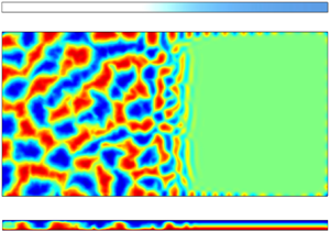
We now examine the convection structures on different vertical planes along  $y$ for
  $\delta =9$. In figures 6(a–c), we show the density plots of vertical velocity on the planes at
  $y=3.4$,
  $y=11.9$ and
  $y=19.7$. The local Hartmann numbers at these locations are
  ${{Ha}}_z(y=3.4)=25$,
  ${{Ha}}_z(y=11.9)=45$ and
  ${{Ha}}_z(y=19.7)=75$. The velocity fluctuations are strong at
  $y=3.4$ where the flow is highly turbulent. At
  $y=11.9$, the flow structures consist of quasi-two-dimensional upward and downward streams occupying the entire plane. The velocity fluctuations become weak at
  $y=19.7$, and the flow structures become elongated along the
  $x$-direction, consistent with the observation from figures 4(e,j). We plot the mean horizontal velocity
  $\left \langle \sqrt {u_x^2 + u_y^2} \right \rangle _x$, the mean absolute vertical velocity
  $\langle |u_z| \rangle _x$, and the mean temperature
  $\langle T \rangle _x$ versus
  $z$ on the above three planes in figures 7(a–c), respectively. These figures further reinstate that the velocity fluctuations decrease along
  $y$. Moreover, the temperature approaches the linear conduction profile as the local magnetic field strength increases.

Figure 6. Contour plots of the time-averaged vertical velocity field for  $\delta =9$ in vertical planes at (a)
  $y=3.4$ (
 ${{Ha}}_z(y)=25$), (b)
  $y=11.9$ (
 ${{Ha}}_z(y)=45$), and (c)
  $y=19.7$ (
 ${{Ha}}_z(y)=75$). The velocity fluctuations decrease with the increasing magnetic field strength along
  $y$.
$y$.

Figure 7. Profiles for  $\delta =9$ of (a) the mean horizontal velocity
 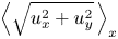 $\left \langle \sqrt {u_x^2+u_y^2} \,\right \rangle _x$, (b) the mean absolute vertical velocity
  $\langle |u_z| \rangle _x$, and (c) the mean temperature along the vertical
  $z$-direction, at
  $y=3.4$ (black dotted curves),
  $y=11.9$ (red dashed curves), and
  $y=19.7$ (blue solid curves). As the magnetic field strength increases along
  $y$, the velocity fluctuations decrease and the temperature approaches the linear conduction profile.
We now analyse quantitatively the isotropy of the flow using our numerical data. Towards this objective, we compute the following ratios: the local vertical anisotropy parameter  $2E_z(y)/E_h(y)$, the local horizontal anisotropy parameter
  $E_y(y)/E_x(y)$, and the ratio of the kinetic energies along the
  $z$- and
  $y$-directions. In these,
  $E_z(y) = 0.5 \langle u_z^2 \rangle _{x,z}$, is the vertical kinetic energy,
  $E_h(y) = 0.5 \langle u_x^2 + u_y^2 \rangle _{x,z}$ is the horizontal kinetic energy,
  $E_x(y) = 0.5 \langle u_x^2 \rangle _{x,z}$ is the kinetic energy along the
  $x$-direction, and
  $E_y(y) = 0.5 \langle u_y^2 \rangle _{x,z}$ is the kinetic energy along the
  $y$-direction, all averaged over the
  $x$–
$x$– $z$ plane. To understand the variation of flow anisotropy with magnetic field strength, the aforementioned anisotropy factors are plotted versus
  ${{Ha}}_z(y)/{{Ha}}_{z,c}$ for different
  $\delta$ in figures 8(a–e). In these plots, we focus on the regions where
  $0.25{{Ha}}_{z,c} < {{Ha}}_z(y) < {{Ha}}_{z,c}$ because, as discussed later, in § 3.2, the flow undergoes significant changes in this parameter interval. Further, we add horizontal tick labels with the coordinates of
  $y$ on the top of each plot to better understand the evolution of anisotropy along the horizontal direction.

Figure 8. Mean profiles of the local vertical anisotropy parameter  $2E_z(y)/E_h(y)$ (solid green curves), the local horizontal anisotropy parameter
  $E_y(y)/E_x(y)$ (dashed red curves), and the ratio of the kinetic energy along the
  $z$- and
  $y$-directions
  $E_z(y)/E_y(y)$ (dotted blue curves), versus the normalized Hartmann number
  ${{Ha}}_z(y)/{{Ha}}_{z,c}$ based on the mean vertical magnetic field
  $B_z(y)$, for (a)
  $\delta =0.01$, (b)
  $\delta =0.3$, (c)
  $\delta =1$, (d)
  $\delta =3$, and (e)
  $\delta =9$. Both the vertical and horizontal anisotropy parameters increase with the local vertical magnetic field strength.
The above plots show that the flow is roughly isotropic in the regions of weak vertical magnetic field corresponding to  ${{Ha}}_z(y)<0.3{{Ha}}_{z,c}$. However, with increasing
  ${{Ha}}_z(y)$, the vertical velocity fluctuations become more dominant compared to the horizontal ones. This property is consistent with the anisotropy observed by Yan et al. (Reference Yan, Calkins, Maffei, Julien, Tobias and Marti2019) and Akhmedagaev et al. (Reference Akhmedagaev, Zikanov, Krasnov and Schumacher2020b) for strong Hartmann number convection with uniform magnetic fields, and is reminiscent of the stable cellular regime described by Zürner et al. (Reference Zürner, Schindler, Vogt, Eckert and Schumacher2020). The increase of anisotropy with
  ${{Ha}}_z(y)$ becomes more pronounced as the fringe width, governed by
  $\delta$, increases. This is because as the fringe width increases, the span of
  $y$ falling in the regime
  $0.25{{Ha}}_{z,c} < {{Ha}}_z(y) < {{Ha}}_{z,c}$ also increases, as exhibited in figures 8(a–e). Thus we get better statistics, and hence clearer trends in this regime for large
  $\delta$.
Figures 8(a–e) also show that for strong magnetic fields, there is anisotropy among the horizontal components of velocity as well. For  ${{Ha}}_z(y)> 0.65 {{Ha}}_{z,c}$,
  $E_y(y)$ begins to dominate
  $E_x(y)$, implying that the velocity fluctuations in the
  $y$-direction are stronger compared to those in the
  $x$-direction. This is also consistent with figures 4(a–j), which show that for moderately strong Hartmann numbers, the superstructure rolls orient themselves perpendicular to the longitudinal sidewalls. In the next subsection, we discuss the effects of the fringing magnetic fields on the local as well as global momentum and heat transport.
3.2. Heat and momentum transport
We analyse the spatial variation of the large-scale heat and momentum transport in our numerical set-up. Towards this objective, we first compute the local planar Reynolds number  ${{Re}}(y)$ and Nusselt number
  ${{Nu}}(y)$ for every
  $\delta$. These are given by
 \begin{equation} {{Re}}(y) = \sqrt{\frac{{{Ra}}}{{{Pr}}}}\langle u_x^2 + u_y^2 + u_z^2 \rangle_{x,z,t_N}^{1/2}, \quad {{Nu}}(y) = 1 + \sqrt{{{Ra}}\,{{Pr}}}\,\langle u_z T \rangle_{x,z,t_N}. \end{equation}
It must be noted that in order to avoid clutter,  ${{Nu}}(y)$ and
  ${{Re}}(y)$ are computed for every 120th
  $x$–
$x$– $z$ plane. Moreover,
  ${{Nu}}(y)$ exhibits strong spatial fluctuations even after averaging over all the time frames; these fluctuations are smoothed by computing the moving average of
  ${{Nu}}(y)$ using a window size of 5
  $x$–
$x$– $z$ planes.
We plot  ${{Nu}}(y)$ and
  ${{Re}}(y)$ versus
  $y$ in figures 9(a) and 9(b), respectively. Figure 9(a) shows that
  ${{Nu}}(y)$ fluctuates between 2.0 and 4.0 in the region of weak magnetic flux, drops steeply in the fringe zone, and becomes close to unity in the strong magnetic flux region. Figure 9(b) shows that
  ${{Re}}(y)$ follows a similar trend; it is large in the weak magnetic flux region, drops steeply in the fringe zone, and becomes negligibly small in the strong magnetic flux region. The gradients of both
  ${{Re}}(y)$ and
  ${{Nu}}(y)$ curves in the fringe zone decrease with an increase of
  $\delta$. This is expected because
  $B_z$, which suppresses kinetic energy and heat transport in the fluid, has steeper gradients for small
  $\delta$.

Figure 9. Variations of the local planar Nusselt and Reynolds numbers with the longitudinal direction  $y$ . For
  $\delta =0.01$–
 $9$: (a) local Nusselt number
  ${{{Nu}}}(y)$, and (b) local Reynolds number
  ${{{Re}}}(y)$, versus
  $y$.
$y$.
We now look for a universal dependence of the local heat and momentum transport on the local magnetic field strength. Taking inspiration from the recent experimental work of Zürner et al. (Reference Zürner, Schindler, Vogt, Eckert and Schumacher2020) on thermal convection under uniform vertical magnetic fields, we plot the normalized local Nusselt number  $\widetilde {{{Nu}}}(y)$ versus the normalized local vertical Hartmann number
  ${{Ha}}_z(y)/{{Ha}}_{z,c}$. The normalized local Nusselt number is given by
 \begin{equation} \widetilde{{{Nu}}}(y) = \frac{{{Nu}}(y)-1}{{{Nu}}_{max}-1}, \end{equation}
where  ${{Nu}}_{max}=2.66$ (see § 2.2). Figure 10(a) shows that for all
  $\delta$, the points collapse well into a single curve, thus showing a universal dependence of
  ${{Nu}}(y)$ on
  ${{Ha}}_z(y)$. The plot shows that for
  ${{Ha}}_z(y)\lesssim 0.3{{Ha}}_{z,c}$, the Nusselt number does not change significantly and remains close to its maximum value. This regime corresponds to the turbulent and isotropic regime. For
  ${{Ha}}_z(y)\gtrsim 0.3{{Ha}}_{z,c}$, the flow transitions into the cellular regime (as per the nomenclature of Zürner et al. Reference Zürner, Schindler, Vogt, Eckert and Schumacher2020) and the local Nusselt number starts to drop sharply as
  ${{Ha}}_z(y)$ increases. For
  ${{Ha}}_z(y)<0.85 {{Ha}}_{z,c}$, the best-fit curve for our data is
 \begin{equation} \widetilde{{{Nu}}}(y) = \left[1 + \chi_1 \left\{\frac{{{Ha}}_z(y)}{{{Ha}}_{z,c}} \right\}^{\gamma_1} \right]^{{-}1}, \end{equation}
where  $\gamma _1 = 2.1 \pm 0.3$ and
  $\chi _1 = 4.0 \pm 0.7$. Interestingly, the values of
  $\chi _1$ and especially
  $\gamma _1$ are close to those observed by Zürner et al. (Reference Zürner, Schindler, Vogt, Eckert and Schumacher2020), who reported
  $\gamma _1 = 2.03 \pm 0.06$ and
  $\chi _1 = 5.9 \pm 0.3$ for uniform magnetic fields. For
  ${{Ha}}_z(y) > 0.85 {{Ha}}_{z,c}$,
  $\widetilde {{{Nu}}}(y)$ decreases more steeply than (3.6) and is described by the power law
 \begin{equation} \widetilde{{{Nu}}}(y) = 0.028 \left\{\frac{{{Ha}}_z(y)}{{{Ha}}_{z,c}} \right\}^{{-}10.5\pm 0.9}. \end{equation}
This regime corresponds to the wall-mode regime in which the flow gets further suppressed and begins to confine itself near the sidewalls. It must be noted that Zürner et al. (Reference Zürner, Schindler, Vogt, Eckert and Schumacher2020) could not obtain a best-fit expression for  ${{Nu}}$ in the wall-mode regime due to lack of data close to the wall.

Figure 10. Variations of the normalized local Nusselt and Reynolds numbers with the normalized local vertical magnetic field strengths. For  $\delta =0.01$–
 $9$: (a) normalized local Nusselt number
  $\widetilde {{{Nu}}}(y)$ versus the normalized local Hartmann number
  ${{Ha}}(y)/Ha_c$, based on vertical magnetic field strength; and (b) normalized local Reynolds number
  $\widetilde {{{Re}}}(y)$ versus the local free-fall interaction parameter
  $N_{f}(y)$. The best-fit curves for the above data are also shown.
We conduct a similar analysis for  ${{Re}}(y)$. We compute the normalized Reynolds number given by
 \begin{equation} \widetilde{{{Re}}}(y) = \frac{{{Re}}(y)}{{{Re}}_{max}}, \end{equation}
where  ${{Re}}_{max}=1115$ (see § 2.2). The results of Zürner et al. (Reference Zürner, Schindler, Vogt, Eckert and Schumacher2020) suggest that
  $\widetilde {{{Re}}}(y)$ should scale as
  ${{Ha}}_z(y)/\sqrt {{{Ha}}_{z,c}}$ instead of
  ${{Ha}}_z(y)/{{Ha}}_{z,c}$. Let us now consider the local free-fall interaction parameter
  $N_{f}(y)$, which is given by
 \begin{equation} N_{f}(y) = {{Ha}}^2_z(y)\,\sqrt{\frac{{{Pr}}}{{{Ra}}}}. \end{equation}
For large Rayleigh numbers, the critical Hartmann number can be approximated as  ${{Ha}}_{z,c} \approx \sqrt {{{Ra}}}/{\rm \pi}$ (Chandrasekhar Reference Chandrasekhar1981). Using this relation, we get
 \begin{equation} N_{f}(y) = {{Ha}}^2_z(y)\,\frac{\rm \pi}{\sqrt{{{Ra}}}}\,\frac{\sqrt{{{Pr}}}}{\rm \pi} \approx \frac{{{Ha}}^2_z(y)}{{{Ha}}_{z,c}}\,\frac{\sqrt{{{Pr}}}}{\rm \pi} \sim \frac{{{Ha}}^2_z(y)}{{{Ha}}_{z,c}}. \end{equation}
This relation shows that  $N_f(y)$ is proportional to
  ${{{Ha}}^2_z(y)}/{{{Ha}}_{z,c}}$, implying that
  $\widetilde {{{Re}}}(y)$ scales with
  $N_f(y)$. Thus we plot
  $\widetilde {{{Re}}}(y)$ versus
  $N_f(y)$. The plot in figure 10(b) shows that, similar to the Nusselt number, the data points for all
  $\delta$ collapse into a single curve. For
  $N_{f}(y) < 0.17$, which corresponds to
  ${{Ha}}_z(y) < 0.22 {{Ha}}_{z,c}$, the Reynolds number retains its maximum value (
 ${{Re}}_{max}$). At higher
  $N_{f}(y)$, the Reynolds number starts to fall sharply with the interaction parameter. For
  $N_{f}(y) < 3.2$, which corresponds to
  ${{Ha}}_z(y) < 0.95 Ha_{z,c}$, the best-fit curve for our data is given by
 \begin{equation} \widetilde{{{Re}}}(y) = \left[1 + \chi_2 \left\{N_{f}(y) \right\}^{\gamma_2} \right]^{{-}1}, \end{equation}
with  $\chi _2 = 1.40 \pm 0.03$ and
  $\gamma _2 = 1.01 \pm 0.03$. The value of
  $\gamma _2$ is again close to that observed by Zürner et al. (Reference Zürner, Schindler, Vogt, Eckert and Schumacher2020), who reported
  $\gamma _2 = 0.87 \pm 0.03$ for uniform magnetic fields. For
  ${{Ha}}_z(y)>0.95 {{Ha}}_{z,c}$, which corresponds to the wall-attached convection regime,
  $\widetilde {{{Re}}}(y)$ falls even more steeply than (3.11) and is described by the power law
 \begin{equation} \widetilde{{{Re}}}(y) = 18\{N_{f}(y)\}^{{-}4.0\pm 0.2}. \end{equation}
 We now analyse the impact of the local heat and momentum transport on the evolution of the viscous and thermal boundary layers near the top and bottom walls of our convection cell. Again, we concentrate on  $\delta =9$ to obtain better statistics and a clearer picture of the evolution. The thermal boundary layer thickness
  $\delta _T$ is the depth where a linear fit of the mean temperature profile near the wall intersects with the mean bulk temperature (
 $T=0.5$). The viscous boundary layer thickness is the depth where a linear fit of the horizontal velocity (
 $u_h = \langle (u_x^2+u_y^2)^{1/2} \rangle _x$) profile near the wall intersects with its local maximum. See Breuer et al. (Reference Breuer, Wessling, Schmalzl and Hansen2004), Ahlers et al. (Reference Ahlers, Grossmann and Lohse2009) and Scheel et al. (Reference Scheel, Kim and White2012) for a detailed procedure to compute the boundary layer thicknesses. We compute the thermal and viscous boundary layer thicknesses at different
  $y$-coordinates for
  $\delta =9$, and plot them versus the corresponding local Hartmann number
  ${{Ha}}_z(y)$ in figures 11(a,b), respectively.

Figure 11. Boundary analysis for  $\delta =9$: (a) local thermal boundary layer thickness
  $\delta _T(y)$, and (b) local viscous boundary layer thickness
  $\delta _u(y)$, near the top and bottom walls, versus the local Hartmann number
  ${{Ha}}_z(y)$. The thermal boundary layer thickness increases with the increase of
  ${{Ha}}_z(y)$. The viscous boundary layer thickness decreases with increasing
  ${{Ha}}_z(y)$ and approaches the Hartmann-type scaling
  $\delta _u \sim {{Ha}}_z^{-1}$ at large Hartmann numbers.
Figure 11(a) shows that the thermal boundary layer thickness increases with  ${{Ha}}_z(y)$. This is expected because the thermal boundary layer thickness is inversely proportional to the local Nusselt number
  ${{Nu}}(y)$, which decreases with increasing
  ${{Ha}}_z(y)$. The viscous boundary layer, on the other hand, exhibits an interesting behaviour. As is evident in figure 11(b), the boundary layer thickness
  $\delta _u$ decreases with
  ${{Ha}}_z(y)$, with the decrease becoming steeper at large
  ${{Ha}}_z(y)$. To gain insight into this behaviour, we take inspiration from the work of Lim et al. (Reference Lim, Chong, Ding and Xia2019), and using dimensional analysis on the momentum equation, we obtain the following scaling for
  $\delta _u$:
 \begin{equation} \delta_u \sim \frac{1}{\sqrt{{{Re}}(y) + {{Ha}}_z^2(y)}}. \end{equation}
This scaling suggests that for  ${{Ha}}_z(y) \ll \sqrt {{{Re}}(y)}$,
  $\delta _u$ follows the Prandtl–Blasius-type scaling
  $\delta _u \sim {{Re}}^{-1/2}$, in which the boundary layer thickness should increase with the decrease of
  ${{Re}}(y)$, and hence with the increase of
  ${{Ha}}_z(y)$. However, we do not observe such a regime in our convection cell. When
  ${{Ha}}_z(y) \sim \sqrt {{{Re}}(y)}$, the boundary layer thickness varies marginally with
  $y$, as observed for
  ${{Ha}}_z(y) < 50$ from our data. For
  ${{Ha}}_z(y) \gg \sqrt {{{Re}}(y)}$, the boundary follows the Hartmann type scaling
  $\delta _u \sim {{Ha}}_z^{-1}$, hence
  $\delta _u$ decreases sharply with
  ${{Ha}}_z(y)$. From figure 11(b), it can be seen that
  $\delta _u$ approaches the Hartmann type scaling at
  ${{Ha}}_z(y) \approx 70$.
Having studied the local variations of heat and momentum transport along with their associated boundary layers, we now analyse the global Reynolds and Nusselt numbers ( ${{Re}}_{global}$ and
  ${{Nu}}_{global}$, respectively) and their dependence on
  $\delta$. These global quantities are computed numerically using (2.12) and (2.13) from our simulation data, and are plotted versus
  $\delta$ in figures 12(a,b) as black squares. The figures show that both
  ${{Re}}_{global}$ and
  ${{Nu}}_{global}$ decrease as
  $\delta$ increases. This result is counter-intuitive because for large
  $\delta$, bulk convection is completely ceased only in a small region (as seen in figure 4), hence one would expect the overall heat and momentum transport to be stronger. However, a careful look at figure 2(a) reveals that the vertical magnetic field is stronger in the weak magnetic flux region for large fringe widths, which, in turn, weakens convection in that region. The increase in convection in the strong magnetic flux region is unable to compensate the suppression of convection in the weak magnetic flux region, resulting in a decrease of overall heat and mass transport for large fringe widths.

Figure 12. Plots versus  $\delta$ of (a) the global Reynolds number
  ${{Re}}_{global}$ (black squares for
  ${{Ha}}_{z,max}=120$ and purple circles for
  ${{Ha}}_{z,max}=30$), computed from our numerical data using (2.12), and (b) the global Nusselt number
  ${{Nu}}_{global}$ (black squares for
  ${{Ha}}_{z,max}=120$ and purple circles for
  ${{Ha}}_{z,max}=30$), computed from our numerical data using (2.13). Also shown in the plots are the estimates (solid curves) of
  ${{Re}}_{global}$ and
  ${{Nu}}_{global}$ computed using (3.14) and (3.15) for different values of
  ${{Ha}}_{z,max}$.
The above results, however, do not indicate whether such a variation of global Reynolds and Nusselt numbers with  $\delta$ holds for all
  ${{Ha}}_{z,max}$. To explore this aspect, we need to estimate
  ${{Re}}_{global}$ and
  ${{Nu}}_{global}$ for given values of
  ${{Ha}}_{z,max}$ and
  $\delta$. Towards this objective, we make use of the best-fit relations for
  ${{Nu}}(y)$ and
  ${{Re}}(y)$ given by (3.6), (3.7), (3.11) and (3.12) obtained earlier, and integrate them numerically over the entire domain to estimate global Reynolds and Nusselt numbers as
 \begin{gather} {{Re}}_{global} = \frac{1}{l_y}\int_0^{l_y} {{Re}}(y)\,{{\rm d} y} = \frac{1}{l_y}\int_0^{l_y} {{Re}}({{Ha}}_z(y))\,{{\rm d} y}, \end{gather}
 \begin{gather}{{Nu}}_{global} = \frac{1}{l_y}\int_0^{l_y} {{Nu}}(y)\,{{\rm d} y} = \frac{1}{l_y}\int_0^{l_y} {{Nu}}({{Ha}}_z(y))\,{{\rm d} y}, \end{gather}
where we recall that
 \begin{equation} {{Ha}}_z(y) = {{Ha}}_{z,max}\,\frac{\langle B_z \rangle_{x,z}}{B_{z,max}}, \end{equation}
and  $B_z=B_z(x,y,z,\delta )$ is given by (2.3). Thus for given
  ${{Ha}}_{z,max}$ and
  $\delta$, one can estimate
  ${{Re}}_{global}$ and
  ${{Nu}}_{global}$ using (3.14) and (3.15). We compute these estimates for
  ${{Ha}}_{z,max}=120$, 60, 50 and 30, and for
  $\delta$ ranging from 0.005 to 9.1 in increments of 0.01. The estimated values of
  ${{Re}}_{global}$ and
  ${{Nu}}_{global}$ are plotted versus
  $\delta$ in figures 12(a,b) as solid curves. The curves for
  ${{Ha}}_{z,max}=120$ fit the data points of directly computed
  ${{Re}}_{global}$ and
  ${{Nu}}_{global}$ (black squares) very well, implying that (3.14) and (3.15) provide fairly accurate estimates. In the process of computing the estimates of
  ${{Re}}_{global}$ and
  ${{Nu}}_{global}$ for
  ${{Ha}}_{z,max} < 120$, we assume that the equations and coefficients given in (3.6), (3.7), (3.11) and (3.12) remain unchanged as the maximum Hartmann number is varied. We also assume that the values
  ${{Ha}}_z(y) = 0.85 {{Ha}}_{z,c}$ and
  $N_f(y)=3.2$, which were observed to separate the two components of the piecewise functions for
  ${{Nu}}(y)$ and
  ${{Re}}(y)$ for
  ${{Ha}}_{z,max}=120$, remain the same for all values of
  ${{Ha}}_{z,max}$. These assumptions are based on the fact that the dependence of
  ${{Nu}}(y)$ and
  ${{Re}}(y)$ on
  ${{Ha}}_z(y)$ is suggested to be universal since the normalized local Nusselt and Reynolds number curves for different
  $\delta$ collapse as shown in figures 10(a,b).
Figure 12(a) also shows that the decrease of  ${{Re}}_{global}$ with
  $\delta$ becomes less apparent with a decrease of
  ${{Ha}}_{z,max}$. In fact, for
  ${{Ha}}_{z,max}=30$,
  ${{Re}}_{global}$ increases marginally with
  $\delta$. Figure 12(b) indicates that
  ${{Nu}}_{global}$ increases with
  $\delta$ for
  ${{Ha}}_{z,max}=60$, 50 and 30, with this increase becoming more apparent with the decrease of
  ${{Ha}}_{z,max}$. To test the correctness of the above predictions, we conduct two more direct numerical simulations of our magnetoconvection set-up for
  ${{Ha}}_{z,max}=30$, and
  $\delta =0.01$ and 9. The grid size and the numerical schemes are the same as those described in § 2.2. We run the simulations for 10 free-fall time units after attaining a statistically steady state. We compute the time-averaged global Reynolds and Nusselt numbers using the above simulation data, and plot them in figures 12(a) and 12(b), respectively. The figures show that the simulation results are in close agreement with the predictions, thereby reinforcing our theory. It is therefore clear that for smaller maximum magnetic field strengths, the overall heat and momentum transport increases with the increase of fringe width. This implies that for small values of
  ${{Ha}}_{z,max}$, the suppression of convection in the weak magnetic flux region is small compared to the increase of convection in the strong magnetic flux region. Thus we can conclude that the variation of
  ${{Re}}_{global}$ and
  ${{Nu}}_{global}$ with the fringe width depends critically on
  ${{Ha}}_{z,max}$. Finally, we discuss the dynamics of wall-attached convection in the strong magnetic flux region in the next subsection.
3.3. Wall-attached convection
We plot the time-averaged isosurfaces of  $u_z = 0.01$ (red) and
  $u_z = -0.01$ (blue) for
  $\delta =1$ and
  $\delta =9$ in figures 13(a) and 13(b), respectively. The figures show that in the strong magnetic flux region, the flow in the bulk is completely suppressed, with alternating upwelling and downwelling flow regions attached to the sidewalls. The structure of the wall modes is consistent with that observed by Liu et al. (Reference Liu, Krasnov and Schumacher2018) in their simulations of thermal convection in a rectangular domain with uniform vertical magnetic field. However, unlike for rotating convection (Horn & Schmid Reference Horn and Schmid2017; Zhang et al. Reference Zhang, van Gils, Horn, Wedi, Zwirner, Ahlers, Ecke, Weiss, Bodenschatz and Shishkina2020) or convection in cylindrical domains (Akhmedagaev et al. Reference Akhmedagaev, Zikanov, Krasnov and Schumacher2020b), the wall modes do not oscillate or move along the sidewalls (Grannan et al. Reference Grannan, Cheng, Aggarwal, Hawkins, Xu, Horn, Sánchez- Álvarez and Aurnou2022; Schumacher Reference Schumacher2022).

Figure 13. Isosurfaces of  $u_z=0.01$ (red) and
  $u_z=-0.01$ (blue) for (a)
  $\delta =1$ and (b)
  $\delta =9$. In the regions with strong magnetic fields, convective motions are confined near the sidewalls.
The wall modes are dense and uniformly distributed along the sidewalls for  $\delta =9$. However, for
  $\delta =1$, they are visibly thinner, with isosurfaces clustering more towards the corners instead of being uniformly distributed along the sidewalls. The clustering occurs because of weaker Lorentz force in the corners, which, in turn, results due to the electric current getting further constrained by the two insulated sidewalls in proximity to each other. The above trend in the local differences of the wall modes is also observed for
  $\delta =0.01$, 0.3 and 3, as shown later in this section.
For each sidewall in the strong magnetic flux region, we compute the mean distance  $\bar {\delta }_w$ of the wall modes from the sidewall. This distance is computed as
 \begin{equation} \bar{\delta}_w = \frac{\displaystyle\int {\delta_w\,u_{z,max}}\,{\rm d}l}{\displaystyle\int {u_{z,max}}\,{\rm d}l}, \end{equation}
where  ${\rm d}l = {{\rm d}y}$ for the longitudinal sidewall, and
  ${\rm d}l = {{\rm d} x}$ for the lateral sidewall. In the above,
  $\delta _w$ is the shortest distance between the sidewall and the point of maximum absolute velocity
  $u_{z,max}$ adjacent to the sidewall, and the summations are over the regions where
  ${{Ha}}_z(y)>{{Ha}}_{z,c}$. Thus
  $\bar {\delta }_w$ is the weighted average of the shortest distance between the point of maximum absolute velocity and the sidewall, with the maximum absolute velocity being the weights. We also compute the mean distance averaged over all the sidewalls. We plot the mean distance for each sidewall, as well as the overall mean distance versus
  $\delta$, in figure 14. The figure shows that the wall modes are in general more attached to the lateral sidewall (
 $y=32$) compared to the longitudinal sidewalls (
 $x=0$ and
  $x=16$). There is, however, no clear trend regarding the variation of
  $\bar {\delta }_w$ with the fringe width.

Figure 14. The average distance between the wall modes and the sidewalls versus  $\delta$ in the regions
  ${{Ha}}_z(y) > {{Ha}}_{z,c}$. The wall modes are more attached to the lateral sidewalls than to the longitudinal sidewalls.
We further analyse the amplitudes of the wall modes along the three sidewalls for our runs. Towards this objective, we measure the vertical velocity field at every point on the horizontal midplane at distance  $\bar {\delta }_w$ from the sidewalls. We plot this vertical velocity profile along every sidewall in figure 15. The figure shows that with the exception of
  $\delta =9$, the amplitudes of the wall modes are stronger near the corners, and become weaker as one moves away from the corners. This behaviour in the amplitudes is consistent with figure 13(a), which shows that the wall modes are clustered in the corners. As explained earlier, these local differences in amplitudes occur due the current being more constrained in the corners, resulting in weaker convection-suppressing Lorentz forces in these regions. Figure 15 also shows that near the corners, the amplitudes of the wall modes grow with an increase of
  $\delta$. However, in the regions away from the corners, the amplitudes decrease as
  $\delta$ is decreased from 9 to 1, and then increase with a further decrease of
  $\delta$. For
  $\delta =0.3$ and 1, the amplitudes become negligibly small away from the corners. However, for
  $\delta =0.01$, although the amplitudes of the modes away from the corners are smaller than those near the corners, they are larger than the amplitudes of wall modes away from the corners for
  $\delta =0.3$ and 1.

Figure 15. Vertical velocity  $u_{z,w}$ measured on the horizontal midplane at distance
  $\bar {\delta }_w$ from the sidewalls in the regions
  ${{Ha}}(y)>{{Ha}}_{z,c}$ (non-shaded regions) for (a)
  $\delta =0.01$ (black curve), (b)
  $\delta =0.3$ (purple curve), (c)
  $\delta =1$ (blue curve), (d)
  $\delta =3$ (green curve), and (e)
  $\delta =9$ (red curve). The shaded regions correspond to
  ${{Ha}}_z(y) < {{Ha}}_{z,c}$, where the flow is not fully suppressed in the bulk. The amplitudes of the wall modes in the regions away from the corners exhibit a non-monotonic dependence on
  $\delta$. Note that these plots are resolved by a total of at least 9000 grid points in the horizontal direction.
The reason for the non-monotonic behaviour of wall modes with  $\delta$ away from the corners is not yet clear. A possible explanation is that in addition to the vertical component of the magnetic field
  $B_z$, the horizontal component
  $B_y$ also plays a role in stabilizing convection near the sidewalls. From figure 2(b), it can be seen that for small
  $\delta$ or fringe width, although
  $B_y$ is strong in
  $y=l_y/2$ midplane, it falls sharply and becomes very small as one moves away from the midplane. Thus for
  $\delta =0.01$,
  $B_y$ is too weak to stabilize convection near the sidewalls at
  $y \gg l_y/2$, resulting in sustained wall-attached convection. On the other hand, for large
  $\delta$,
  $B_y$ in the regions away from
  $y=l_y/2$ midplane is not as weak as that for small
  $\delta$. Thus as
  $\delta$ is increased up to
  $\delta =1$,
  $B_y$ becomes stronger and suppresses wall-attached convection. On further increasing
  $\delta$, although
  $B_y$ grows only marginally,
  $B_z$ becomes too weak to suppress wall-attached convection. Hence we get prominent wall modes again for
  $\delta =3$ and 9. The non-monotonic behaviour of wall modes will be explored in detail in a future study.
4. Summary and conclusions
In this paper, we performed detailed numerical simulations of turbulent convection of a horizontally extended domain under the influence of fringing magnetic fields. The magnetic field is generated in the gap between semi-infinite poles of permanent magnets, with the convection domain located near the edge of the gap. The quasi-static approximation of magnetohydrodynamics is applied. We kept the Rayleigh number, Prandtl number and maximum Hartmann number fixed at  ${{Ra}}=10^5$,
  ${{Pr}}=0.021$ and
  ${{Ha}}_{z,max}=120$, respectively, and varied the fringe width by controlling the gap
  $\delta$ between the magnetic poles and the thermal plates. We analysed the spatial distribution of large-scale convection patterns, heat and momentum transport, and wall-attached convection, and their variations with the magnetic field profiles.
The convection patterns are found to be comprised of structures whose horizontal dimensions are larger than the domain height. These structures do not exhibit any preferred orientation in regions of weak magnetic field, but become aligned perpendicular to the longitudinal sidewalls in the fringe zone. Further, the flow progressively becomes anisotropic towards the vertical direction in the fringe zone.
We obtained the best-fit relations for local Reynolds and Nusselt numbers as functions of the local Hartmann number that are valid for any fringe width. We integrated these relations over the entire domain to estimate the global Reynolds and Nusselt numbers for different values of  ${{Ha}}_{z,max}$. The variation of these global quantities with fringe width was shown to depend on
  ${{Ha}}_{z,max}$ and is governed by the balance between the convective motion in the weak magnetic flux region outside the gap between the magnets, and suppression of convection in the strong magnetic flux region inside the gap between the magnets. As the fringe width increases, the magnetic field becomes weaker in the strong magnetic flux region; it becomes stronger in the weak magnetic flux region. For large
  ${{Ha}}_{z,max}$, the increase of convection in the strong magnetic field region is unable to compensate for the suppression of convection in the weak magnetic flux region, resulting in a decrease of the global heat and momentum transport with increasing fringe width. However, for small
  ${{Ha}}_{z,max}$, the increase of convection in the strong magnetic field region is more than the decrease of convection in the weak magnetic flux region, resulting in an increase of global heat and momentum transport with increasing fringe width.
We further analysed wall-attached convection in the regions of strong magnetic flux. We showed that the amplitudes of the wall modes away from the corners decrease when  $\delta$ is decreased from 9 to 1, but begin to increase on further reduction of
  $\delta$. We believe that the horizontal components of the magnetic field play a crucial role in the stability of the wall modes. A detailed study on the this behaviour will be conducted in a future work.
Here, we also remark that the initial conditions play a minor role in the evolution of the large-scale structures. In the Appendix, therefore, we compare some of our results for  $\delta =9$ with another simulation of the same set-up with identical parameters, but different initial conditions. We observe that although there is a marginal difference in the alignment of the superstructures, the other results, such as the global Nusselt and Reynolds numbers, and the variations of anisotropy and the local heat transport along
  $y$, remain largely unchanged.
Our present work provides important insights into the dynamics of thermal convection under spatially varying magnetic fields, which may find applications in several industrial and astrophysical flows. It should therefore be considered as a first step towards understanding thermally driven flows in applications where non-homogeneous magnetic fields are encountered. For example, our results are expected to help in designing engineering applications such as cooling blankets in fusion reactors. Although we worked on a small set of parameters, we expect our results to hold for higher Rayleigh numbers as well. In the future, we plan to conduct a similar analysis for fluids at different Prandtl numbers.
Acknowledgements
The authors thank A. Pandey, Y. Kolesnikov, M. Brynjell-Rahkola, M.K. Verma and A. Ranjan for useful discussions. The authors are grateful to the anonymous referees for their suggestions on improving the paper. The authors gratefully acknowledge the computing time provided to them on the high-performance computer Noctua2 at the NHR Center PC $^2$ of Paderborn University (Germany). These are funded by the Federal Ministry of Education and Research and the state governments participating on the basis of the resolutions of the GWK for national high-performance computing at universities (www.nhr-verein.de/unsere-partner). The authors further acknowledge the computing time provided by Leibniz Supercomputing Center, Garching, Germany, under the projects ‘pn49ma’ and ‘pn68ni.’ The authors thank the Computing Center of Technische Universität Ilmenau for the resources provided to them for postprocessing and visualization of their simulation data.
Funding
The work of S.B. is sponsored by a postdoctoral fellowship of the Alexander von Humboldt Foundation, Germany.
Declaration of interests
The authors report no conflict of interest.
Appendix. Effect of initial conditions
In this appendix, we explore the impact of initial conditions on the solutions in our convection set-up as described in § 2. In the present work, all the simulations were initialized with the conduction profile for temperature and a small perturbation of amplitude  $A=0.001$ in the
  $z$-direction for velocity. Here, we consider another simulation of our set-up for
  $\delta =9$,
  ${{Ha}}_{z,max}=120$, but with the pure convective state solution (i.e. the solution for
  ${{Ha}}_{z,max}=0$) as the initial condition. Like the previous runs, this simulation was initially run on a coarse grid of
  $480 \times 960 \times 30$ points for 100 free-fall time units in which it converged to a statistically steady state. Following this, the mesh was refined successively to the resolution
  $4800 \times 9600 \times 300$ grid points, and the simulation was allowed to converge after each refinement. Once the simulation reached the statistically steady state at the highest resolution, it was run for a further 21 free-fall time units, and a snapshot was saved after every free-fall time unit. Henceforth, we refer to this simulation as IC 2, and the earlier simulation for
  $\delta =9$ (with the quiescent state being the initial condition) as IC 1.
In figures 16(a–c), we show contour plots of vertical velocity  $u_z$ on the horizontal midplane for IC 2 at three different snapshots corresponding to
  $t=0$,
  $9$ and
  $18$, respectively; here,
  $t$ is measured from the time stamp of the first snapshot. In figure 16(d), we show the density plot of
  $u_z$ averaged over 21 free-fall time units. For comparison, we also exhibit the contour plot of vertical velocity on the horizontal midplane for IC 1. In figures 16(e–g), the plots correspond to the snapshots at
  $t=0$,
  $9$ and
  $18$, respectively, where
  $t$ is measured from the time stamp of the first snapshot. Figure 16(h) exhibits the density plot of vertical velocity averaged over 20 free-fall time units. All the figures show that the large-scale patterns are qualitatively similar in the weak magnetic flux region for both IC 1 and IC 2. In the fringe zone, however, there is a difference in the alignment of the superstructures, with the reorientation of the patterns perpendicular to the longitudinal sidewalls being more prominent for IC 1. Further, in the region where
  ${{Ha}}_z \approx {{Ha}}_{z,c}$, convection is suppressed completely in the bulk for IC 1, but some traces of convection are still present for IC 2. We remark that minor effects of initial conditions on magnetohydrodynamic flows have already been observed in the past; see, for example, Sukoriansky, Zilberman & Branover (Reference Sukoriansky, Zilberman and Branover1986) and Zikanov et al. (Reference Zikanov, Krasnov, Boeck and Sukoriansky2019).

Figure 16. Contour plots of vertical velocity  $u_z$ for
  $\delta =9$ in the horizontal midplane for different initial conditions. For the simulation IC 2, contour plots of
  $u_z$ at (a)
  $t=0$, (b)
  $t=9$, and (c)
  $t=18$, where
  $t$ is measured from the time stamp of the first snapshot saved at statistically steady state. For the simulation IC 1, contour plots of
  $u_z$ at (e)
  $t=0$, (f)
  $t=9$, and (g)
  $t=18$, where
  $t$ is measured from the time stamp of the first snapshot saved at statistically steady state. Contour plots of time-averaged vertical velocity for (d) IC 2 and (h) IC 1. The positions corresponding to
  ${{Ha}}_z(y)={{Ha}}_{z,c}$,
  ${{Ha}}_z(y)=0.8 {{Ha}}_{z,c}$ and the edge of the magnetic poles are represented by purple, blue and black horizontal lines, respectively, in decreasing order of thickness. The magnetic poles extend from
  $y=16$ to
  $y=\infty$.
We compute the planar kinetic energy ( $E(y) = 0.5 \langle u_x^2 + u_y^2 + u_z^2 \rangle _{x,z}$), the local vertical anisotropy parameter (
 $2E_z(y)/E_h(y)$), the local horizontal anisotropy parameter (
 $E_y(y)/E_x(y)$), and the ratio of the kinetic energies along the
  $z$- and
  $y$-directions for IC 1 and IC 2. The aforementioned anisotropy parameters are defined in § 3.1. We plot the above quantities versus the local Hartmann number in figures 17(a–d). Figure 17(a) shows that the
  $E(y)$–
 ${{Ha}}_z(y)$ curves for IC 1 and IC 2 collapse, implying that the local variations of kinetic energy do not change with the initial conditions. From figures 17(b–d), it is clear that although the curves of the anisotropy factors for the two different initial conditions do not collapse, they still follow the same trend. Similar to IC 1, the vertical velocity fluctuations for IC 2 become stronger compared to the horizontal ones with the increase of
  ${{Ha}}_z(y)$. Further, for both IC 1 and IC 2, the velocity fluctuations in the
  $y$-direction become stronger compared to those in the
  $x$-direction as
  ${{Ha}}_z(y)$ increases.

Figure 17. For  $\delta =9$ and different initial conditions: mean profiles of (a) the local kinetic energy
  $E(y)$, (b) the local vertical anisotropy parameter
  $2E_z(y)/E_h(y)$, (c) the local horizontal anisotropy parameter
  $E_y(y)/E_x(y)$, and (d) the ratio of the kinetic energy along the
  $z$- and
  $y$-directions, versus the Hartmann number,
  ${{Ha}}_z(y)$, based on the mean vertical magnetic field
  $B_z(y)$. For both sets of initial conditions, the variations of
  $E(y)$ with
  ${{Ha}}_z(y)$ are identical, and the anisotropy parameters increase with the local vertical magnetic field strength.
We plot the normalized local Nusselt number  $\widetilde {{{Nu}}}(y)$ versus the normalized local vertical Hartmann number
  ${{Ha}}_z(y)/{{Ha}}_{z,c}$ for both sets of initial conditions in figure 18(a). For the above data, we also plot the normalized Reynolds number
  $\widetilde {{{Re}}}(y)$ versus the local free-fall interaction parameter
  $N_f(y)$ in figure 18(b). The quantities
  $\widetilde {{{Nu}}}(y)$,
  $\widetilde {{{Re}}}(y)$ and
  $N_f(y)$ are defined in (3.5), (3.8) and (3.10), respectively. Figures 18(a,b) show that both
  $\widetilde {{{Nu}}}(y)$ and
  $\widetilde {{{Re}}}(y)$ for the two different initial conditions collapse well, showing that the dependence of the above quantities on the local magnetic field is independent of the initial conditions. The time-averaged global Nusselt and Reynolds numbers for IC 2 are calculated to be
  ${{Nu}}_{global}=2.60$ and
  ${{Re}}_{global}=479$. These values are nearly identical to those for IC 1, where
  ${{Nu}}_{global}=2.60$ and
  ${{Re}}_{global}=474$.

Figure 18. Variations of the normalized local planar Nusselt and Reynolds numbers with the normalized local vertical magnetic field strengths. For IC 1 and IC 2: (a) normalized local Nusselt number  $\widetilde {{{Nu}}}(y)$ versus the normalized local Hartmann number
  ${{Ha}}(y)/Ha_c$, based on vertical magnetic field strength; and (b) normalized local Reynolds number
  $\widetilde {{{Re}}}(y)$ versus the local free-fall interaction parameter
  $N_{f}(y)$.
Our results show that although the initial conditions can have some impact on the size and alignment of the convection patterns in the fringe zone, they do not alter the global heat and momentum transport, the local variations of heat and momentum transport, and the trend in the variations of local anisotropy.


 Open access