


1. Introduction
Despite the complex and often chaotic dynamics exhibited by many unsteady fluid flows, in many cases it is dominated by energetic coherent structures evolving on relatively long length and time scales (Holmes, Lumley & Berkooz Reference Holmes, Lumley and Berkooz1996). This realization made it possible to study fluid flows as high-dimensional dynamical systems evolving on a low-dimensional manifold, providing answers to longstanding questions on topics such as the route to turbulence (Landau Reference Landau1944; Hopf Reference Hopf1948; Ruelle & Takens Reference Ruelle and Takens1971; Swinney & Gollub Reference Swinney and Gollub1981) and the role of nonlinear interactions (Landau Reference Landau1944; Stuart Reference Stuart1958). The persistent nature of these coherent structures eventually also raised the possibility of using low-dimensional surrogate models for optimization and control objectives (Noack, Morzynski & Tadmor Reference Noack, Morzynski and Tadmor2011; Brunton & Noack Reference Brunton and Noack2015; Rowley & Dawson Reference Rowley and Dawson2017).
The fundamental challenges in constructing such reduced-order models may be broken into two categories: approximating the structures themselves, and approximating their evolution. We refer to these as the kinematic and dynamic approximations, respectively. A modal separation of variables assumption is often employed for the former task (Taira et al. Reference Taira, Brunton, Dawson, Rowley, Colonius, McKeon, Schmidt, Gordeyev, Theofilis and Ukeiley2017, Reference Taira, Hemati, Brunton, Sun, Duraisamy, Bagheri, Dawson and Yeh2020), but although this may be suitable for many closed or diffusion-dominated flows, it is not a natural representation of travelling waves or advection-dominated flows (Rowley & Marsden Reference Rowley and Marsden2000; Reiss et al. Reference Reiss, Schulze, Sesterhenn and Mehrmann2018; Rim, Moe & LeVeque Reference Rim, Moe and LeVeque2018; Grimberg, Farhat & Youkilis Reference Grimberg, Farhat and Youkilis2020; Mendible et al. Reference Mendible, Brunton, Aravkin, Lowrie and Kutz2020). This issue is inextricably linked to the problem of modelling the coherent structure dynamics; as is well known in many domains, a proper choice of coordinates can greatly simplify the modelling task (Champion et al. Reference Champion, Lusch, Kutz and Brunton2019).
The multiscale nature of fluid flows further complicates both the kinematic and dynamic aspects of low-dimensional modelling. For instance, the effective dimensionality of a chaotic flow well above the threshold of instability may be orders of magnitude greater than that of a laminar flow with one or two instability modes. Meanwhile, the ‘triadic’ structure of the nonlinear interactions in the wavenumber or frequency domain ensures that the dynamics of all scales across the flow is linked. Thus, even if the large, energetic coherent structures can be approximated with a low-dimensional basis, models of their dynamics that do not account for the role played by the unresolved degrees of freedom are often unstable or physically inconsistent (Noack et al. Reference Noack, Morzynski and Tadmor2011; Callaham et al. Reference Callaham, Loiseau, Rigas and Brunton2021). Similar considerations impact the development of numerical methods (Bazilevs et al. Reference Bazilevs, Calo, Cottrell, Hughes, Reali and Scovazzi2007), self-consistent mean flow modelling (Meliga Reference Meliga2017) and resolvent analysis (Padovan, Otto & Rowley Reference Padovan, Otto and Rowley2020; Rigas, Sipp & Colonius Reference Rigas, Sipp and Colonius2021; Barthel, Zhu & McKeon Reference Barthel, Zhu and McKeon2021; Barthel, Gomez & McKeon Reference Barthel, Gomez and McKeon2022).
The need for subscale modelling was apparent even in early work combining empirical modal approximations, such as the proper orthogonal decomposition (POD), with physics-based model reduction, such as Galerkin projection. For example, low-dimensional models of vortex shedding in the globally unstable cylinder wake could accurately predict the dynamics over short times, but were subject to structural instability over a longer time horizon (Deane et al. Reference Deane, Kevrekedis, Karniadakis and Orszag1991; Ma & Karniadakis Reference Ma and Karniadakis2002). Eventually, Noack et al. (Reference Noack, Afanasiev, Morzynski, Tadmor and Thiele2003) showed that this was a result of the failure of the standard post-transient POD basis to resolve the Stuart–Landau mechanism of mean-flow deformation associated with nonlinear interactions between the fluctuations (Landau Reference Landau1944; Stuart Reference Stuart1958), an insight that enabled low-dimensional modelling of natural and actuated flows with an increasingly complex dynamics (Luchtenburg et al. Reference Luchtenburg, Günther, Noack, King and Tadmor2009; Deng et al. Reference Deng, Noack, Morzynski and Pastur2020; Sieber, Paschereit & Oberleithner Reference Sieber, Paschereit and Oberleithner2021; Callaham et al. Reference Callaham, Rigas, Loiseau and Brunton2022; Deng et al. Reference Deng, Noack, Morzyński and Pastur2021).
Contemporary work on POD–Galerkin modelling of turbulent shear flows also recognized the need for closure models that could approximate the effect of unresolved scales (Aubry et al. Reference Aubry, Holmes, Lumley and Stone1988; Rempfer & Fasel Reference Rempfer and Fasel1994; Ukeiley et al. Reference Ukeiley, Cordier, Manceau, Delville, Glauser and Bonnet2001). These efforts targeted two distinct physical mechanisms: mean-flow deformation and subscale dissipation. For flows that are either parallel (Aubry et al. Reference Aubry, Holmes, Lumley and Stone1988) or weakly non-parallel under the assumption of Taylor's frozen turbulence hypothesis (Ukeiley et al. Reference Ukeiley, Cordier, Manceau, Delville, Glauser and Bonnet2001), these authors developed a Boussinesq eddy viscosity relationship between the resolved scales and a slowly varying parallel mean flow, leading to stabilizing cubic terms consistent with the Stuart–Landau description. To capture dissipation due to the unresolved scales, these models also adopted a linear mixing length approximation.
Although these studies remain landmark explorations of low-dimensional coherent structure modelling, there are several opportunities to improve the proposed closure strategies. First, it is difficult to generalize the Reynolds stress models applied to parallel shear flows by Aubry et al. (Reference Aubry, Holmes, Lumley and Stone1988) and Ukeiley et al. (Reference Ukeiley, Cordier, Manceau, Delville, Glauser and Bonnet2001) to fully inhomogeneous flows. While the ‘shift mode’ approach to mean flow modelling via an augmented POD basis introduced by Noack et al. (Reference Noack, Afanasiev, Morzynski, Tadmor and Thiele2003) is agnostic to the geometry of the flow, it requires computation of the unstable steady state of the Navier–Stokes equations, which is not generally experimentally accessible. Second, in the Richardson–Kolmogorov energy cascade description, energy is transferred from large to small scales through nonlinear interactions, where it is finally dissipated. This is not consistent with a linear mixing length model, a fact exploited by later work investigating nonlinear models of subscale dissipation (Wang et al. Reference Wang, Akhtar, Borggard and Iliescu2012; Cordier et al. Reference Cordier, Noack, Tissot, Lehnasch, Delville, Balajewicz, Daviller and Niven2013; Östh et al. Reference Östh, Noack, Krajnovic̀, Barros and Borèe2014), particularly the finite time thermodynamics approach, which is centred on modelling unresolved nonlinear energy transfers (Noack et al. Reference Noack, Schlegel, Ahlborn, Mutschke, Morzynski, Comte and Tadmor2008).
Recent years have seen a surge in interest in data-driven and machine learning-based methods (Brenner, Eldredge & Freund Reference Brenner, Eldredge and Freund2019; Duraisamy, Iaccarino & Xiao Reference Duraisamy, Iaccarino and Xiao2019; Brunton, Noack & Koumoutsakos Reference Brunton, Noack and Koumoutsakos2020), including a number of proposed closure and stabilization schemes for reduced-order models, either through regression to additional linear–quadratic terms (Mohebujjaman et al. Reference Mohebujjaman, Rebholz, Xie and Iliescu2017; Mohebujjaman, Rebholz & Iliescu Reference Mohebujjaman, Rebholz and Iliescu2018; Xie et al. Reference Xie, Mohebujjaman, Rebholz and Iliescu2018) or by adding a deep learning model to approximate the residual (San & Maulik Reference San and Maulik2018a,Reference San and Maulikb; Menier et al. Reference Menier, Bucci, Yagoubi, Mathelin and Schcoenauer2022). Alternative work has explored interpretable system identification methods that forego the projection-based model altogether (Brunton, Proctor & Kutz Reference Brunton, Proctor and Kutz2016; Peherstorfer & Willcox Reference Peherstorfer and Willcox2016; Loiseau & Brunton Reference Loiseau and Brunton2018; Qian et al. Reference Qian, Kramer, Peherstorfer and Willcox2020; Callaham et al. Reference Callaham, Rigas, Loiseau and Brunton2022), but may incorporate physical constraints derived from the Galerkin system (Loiseau, Noack & Brunton Reference Loiseau, Noack and Brunton2018b; Deng et al. Reference Deng, Noack, Morzynski and Pastur2020; Kaptanoglu et al. Reference Kaptanoglu, Callaham, Hansen, Aravkin and Brunton2021a). If an accurate, non-intrusive model is more important than interpretability or satisfying physical constraints, then the traditional projection-based framework can be eliminated altogether with black-box neural network forecasting methods (Hesthaven & Ubbiali Reference Hesthaven and Ubbiali2018; Wan et al. Reference Wan, Vlachas, Koumoutsakos and Sapsis2018).
These empirical closure models are constructed on the assumption that the influence of the unresolved variables can be approximated based on information from the resolved variables alone. The success of the Reynolds stress–mean-flow models (Aubry et al. Reference Aubry, Holmes, Lumley and Stone1988; Ukeiley et al. Reference Ukeiley, Cordier, Manceau, Delville, Glauser and Bonnet2001; Manti $\breve{c}$-Lugo, Arratia & Gallaire Reference Mantic-Lugo, Arratia and Gallaire2014), invariant or centre manifold reductions (Coullet & Spiegel Reference Coullet and Spiegel1983; Guckenheimer & Holmes Reference Guckenheimer and Holmes1983; Noack et al. Reference Noack, Afanasiev, Morzynski, Tadmor and Thiele2003; Carini, Auteri & Giannetti Reference Carini, Auteri and Giannetti2015) and weakly nonlinear analysis (Stuart Reference Stuart1958; Sipp & Lebedev Reference Sipp and Lebedev2007; Meliga, Chomaz & Sipp Reference Meliga, Chomaz and Sipp2009; Meliga & Chomaz Reference Meliga and Chomaz2011) suggests that there may be circumstances where this relationship may be derived analytically via traditional analysis. The unifying thread between these methods is the assumption of a scale separation between the resolved and unresolved variables that can be exploited to develop an asymptotically correct closure model.
Beyond the field of fluid dynamics, the method of adiabatic elimination (Haken Reference Haken1983; Risken Reference Risken1996) has long been used to discard the fast variables in systems with emergent large-scale coherence when there is a separation in time scales, while heterogeneous multiscale methods have played an important role in simulating physical systems with widely separated scales (Weinan & Engquist Reference Weinan and Engquist2003; Weinan et al. Reference Weinan, Engquist, Li, Ren and Vanden-Eijnden2007; Weinan Reference Weinan2011). A similar stochastic averaging approach has been successful in climate modelling (Majda, Timofeyev & Vanden-Eijnden Reference Majda, Timofeyev and Vanden-Eijnden2001), where the primitive equations have the same quadratic nonlinearity as the usual Navier–Stokes equations without rotation, buoyancy, topography, etc. This method, also called homogenization in the multiscale modelling literature, has its roots in the theory of singular perturbations of Markov processes (Kurtz Reference Kurtz1973; Papanicolaou Reference Papanicolaou1976) and is rigorously supported for stochastic systems with asymptotic scale separation; see Majda et al. (Reference Majda, Timofeyev and Vanden-Eijnden2001), Givon, Kupferman & Stuart (Reference Givon, Kupferman and Stuart2004), Weinan (Reference Weinan2011) or Pavliotis & Stuart (Reference Pavliotis and Stuart2012) for in-depth presentations. With some assumptions on ergodicity, a similar approach can also be taken with deterministic systems, even in a regime where the scale separation is not in the asymptotic limit (Majda, Timofeyev & Vanden-Eijnden Reference Majda, Timofeyev and Vanden-Eijnden2006).
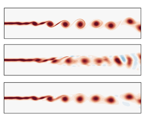
This work explores the application of multiscale stochastic averaging methods developed by Majda et al. (Reference Majda, Timofeyev and Vanden-Eijnden2001), Givon et al. (Reference Givon, Kupferman and Stuart2004), Weinan (Reference Weinan2011), Pradas et al. (Reference Pradas, Pavliotis, Kalliadasis, Papageorgiou and Tseluiko2012), Pavliotis & Stuart (Reference Pavliotis and Stuart2012) and others to the closure problem in reduced-order models of incompressible flow or other systems reducible to a linear–quadratic dynamics (Rowley, Colonius & Murray Reference Rowley, Colonius and Murray2004; Qian et al. Reference Qian, Kramer, Peherstorfer and Willcox2020; Kaptanoglu et al. Reference Kaptanoglu, Morgan, Hansen and Brunton2021b), including introducing an approximation to the form of the fast dynamics that allows for computation of the averaged dynamics in closed form. When applied to a Galerkin model of incompressible flow, this procedure effectively approximates nonlinear energy transfers to unresolved scales by higher-order nonlinearities in the resolved dynamics, as illustrated by figure 1 and illustrated schematically by figure 2. We refer to this secondary dimensionality reduction of the Galerkin system as MMR. Although dynamically complex fluid flows often exhibit structure across a wide range of spatio-temporal scales, in the present context the term multiscale refers specifically to the asymptotic time-scale separation assumed formally by the averaging procedure and does not imply anything about the spectral content of any particular flow.

Figure 1. Multiscale closure model applied to a mixing layer. The visualization of the network of average quadratic energy transfer between the leading harmonic modes shows the cascade of energy to higher-order modes. The multiscale model reduction (MMR) method approximates the effects of unresolved higher-order modes via stochastic averaging, which leads to a generalized Stuart–Landau-type equation with cubic nonlinear interactions. The network visualization of quadratic energy transfers (left) is computed from the modal coefficients  $\boldsymbol a(t)$ and Galerkin model for the leading harmonics, while that of the multiscale approximation (right) is a notional illustration of the origin of the cubic terms in (4.18b). See § 6.3 for details on the construction of this figure and the low-dimensional model of the mixing layer.
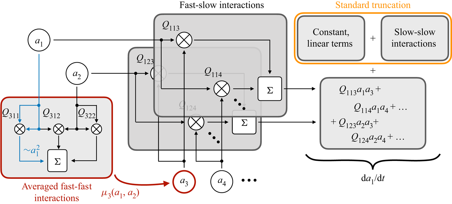
Figure 2. Schematic of nonlinear interactions in the multiscale closure scheme. The dynamics of one variable ( $a_1$) in a system with two slow variables involves quadratic interactions between fast and slow variables that would be neglected in a standard truncation. Instead, the proposed method averages over the fast scales, ultimately generating effective cubic nonlinearities in the closed equations. The quadratic interactions $Q$ represent terms that might arise for instance from Galerkin projection via (2.6c).
Since fluid flows generally do not have a true scale separation away from the threshold of instability, we demonstrate via numerical simulations that this method is a robust and systematic approach to stabilizing low-dimensional models. This extends the work of Majda et al. (Reference Majda, Timofeyev and Vanden-Eijnden2006) exploring the application of this class of methods to systems beyond the parameter regimes where their validity can be rigorously proven. Multiscale model reduction is a unified framework for understanding the origin and importance of cubic terms in reduced-order models of the linear–quadratic Navier–Stokes equations, capable of capturing both mean-flow deformation and subscale dissipation. Throughout this work we also highlight connections to other modelling methods, including Koopman theory and weakly nonlinear analysis.
2. Reduced-order modelling for incompressible flows
For more than three decades, POD and Galerkin projection have been the foundational tools in low-order modelling for nonlinear incompressible fluid flow. The POD analysis identifies dominant coherent structures in the flow and provides an energy-optimal linear modal basis. Galerkin projection approximates both the state of the flow and its time derivative in this finite-dimensional subspace, resulting in a reduced system of ordinary differential equations in terms of the POD mode amplitudes. These topics have been covered extensively elsewhere (see e.g. Holmes et al. Reference Holmes, Lumley and Berkooz1996; Noack et al. Reference Noack, Morzynski and Tadmor2011; Benner, Gugercin & Willcox Reference Benner, Gugercin and Willcox2015; Rowley & Dawson Reference Rowley and Dawson2017; Taira et al. Reference Taira, Brunton, Dawson, Rowley, Colonius, McKeon, Schmidt, Gordeyev, Theofilis and Ukeiley2017); here, we provide a brief overview.
We assume the flow is governed by the unsteady incompressible Navier–Stokes equations
 \begin{equation} \left.\begin{gathered} \frac{\partial \boldsymbol{u}}{\partial t} + \boldsymbol{\nabla} \boldsymbol{\cdot} \left( \boldsymbol{u} \otimes \boldsymbol{u} \right) ={-} \boldsymbol{\nabla} p + \frac{1}Re \nabla^2 \boldsymbol{u} \\ \boldsymbol{\nabla} \boldsymbol{\cdot} \boldsymbol{u} = 0, \end{gathered}\right\} \end{equation}
where  $\boldsymbol {u}(\boldsymbol {x}, t)$ is the velocity field, $p$ is the pressure field and $Re$ is the Reynolds number, $Re =UL / \nu$, based on the kinematic viscosity $\nu$ and suitable length and velocity scales $L$ and $U$. The nonlinear term is expressed in divergence form with the tensor product $\otimes$. In this work, we only consider two dimensional examples for which $\boldsymbol u = [u \enspace v]^\textrm {T}$, although all of the following applies equally well to three-dimensional flows.
In order to reduce the system of partial differential equations (PDEs) (2.1) to a finite-dimensional system of ordinary differential equations, we assume that the space and time dependence can be separated, so that an arbitrary velocity field  $\boldsymbol u(\boldsymbol x, t)$ can be approximated with the $r$-dimensional modal representation
 \begin{equation} \boldsymbol u(\boldsymbol x, t) \approx \boldsymbol{\psi}_0(\boldsymbol x) + \sum_{i=1}^r \boldsymbol \psi_i(\boldsymbol x) a_i(t), \end{equation}
where  $\boldsymbol {\psi }_0(\boldsymbol x)$ is a fixed base flow around which the expansion is performed and each mode individually satisfies the divergence-free constraint $\boldsymbol {\nabla }\boldsymbol {\cdot } \boldsymbol {\psi }_i = 0$ for $i=0, 1, 2, \ldots, r$. Unless otherwise specified we will take $\boldsymbol {\psi }_0$ to be the mean flow $\bar {\boldsymbol u}$ as estimated with a time average.
The POD identifies the set of modes  $\{\boldsymbol {\psi }_i\}_{i=1}^r$ that provide the optimal rank- $r$ approximation for an average velocity field in the energy norm induced by the velocity inner product
 \begin{equation} \langle \boldsymbol u_1, \boldsymbol u_2 \rangle = \int_\varOmega \boldsymbol u_1(\boldsymbol x) \boldsymbol{\cdot} \boldsymbol u_2(\boldsymbol x)\,{\textrm d} \varOmega, \end{equation}
defined on the spatial domain  $\varOmega$ for real-valued velocity fields $\boldsymbol u_1$ and $\boldsymbol u_2$. We approximate this integral with a weighted sum $\langle \boldsymbol u_1, \boldsymbol u_2 \rangle \approx \boldsymbol{\mathsf{u}}_1^\textrm {T} \boldsymbol{\mathsf{W}} \boldsymbol{\mathsf{u}}_2,$ where $\boldsymbol{\mathsf{u}}_1$ and $\boldsymbol{\mathsf{u}}_2$ are the discrete approximations to $\boldsymbol u_1$ and $\boldsymbol u_2$, and $\boldsymbol{\mathsf{W}}$ is a diagonal weight matrix containing the cell volumes. We estimate the POD modes from the two-point temporal correlation matrix using the method of snapshots (Sirovich Reference Sirovich1987).
The POD expansion (2.2) is often only applied to the velocity fields. This can pose a problem for model reduction methods approximating the pressure gradient term in the Navier–Stokes equations. While this term vanishes for closed flows and is often negligible for flows with a localized global instability, it is important in open shear flows, such as the mixing layer examined in § 6 (Noack, Papas & Monkewitz Reference Noack, Papas and Monkewitz2005). There are various methods for approximating the pressure term (see e.g. Caiazzo et al. Reference Caiazzo, Iliescu, John and Schyschlowa2014), but in this work we use a velocity–pressure expansion with the same inner product (2.3). Defining  $\boldsymbol q(\boldsymbol x, t) = [\boldsymbol u \enspace p]^\textrm {T}$, we replace (2.2) and (2.3) with
 \begin{align} \boldsymbol q(\boldsymbol x, t) &\approx \begin{bmatrix} \boldsymbol \psi^{\boldsymbol u}_0(\boldsymbol x) \\ \psi^p_0(\boldsymbol x) \end{bmatrix} + \sum_{i=1}^r \begin{bmatrix} \boldsymbol \psi^{\boldsymbol u}_i(\boldsymbol x) \\ \psi^p_i(\boldsymbol x) \end{bmatrix} a_i(t) \end{align}
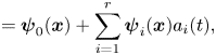 \begin{align} &= \boldsymbol{\psi}_0(\boldsymbol x) + \sum_{i=1}^r \boldsymbol \psi_i(\boldsymbol x) a_i(t), \end{align}
and energy inner product  $\langle \boldsymbol q_1, \boldsymbol q_2 \rangle _{\boldsymbol u} \equiv \langle \boldsymbol u_1, \boldsymbol u_2 \rangle$. Numerically, we simply carry the pressure fields through the method of snapshots by setting the diagonal entries of $\boldsymbol{\mathsf{W}}$ corresponding to pressure to zero. The pressure components of the POD modes are therefore estimated from the same linear combination of snapshots as the velocity components.
The derivation of the Galerkin system proceeds by substituting the velocity–pressure POD approximation (2.4) into the Navier–Stokes equations (2.1). In order for the dynamics to be an optimal continuous-time approximation, the residual error should be orthogonal to the POD subspace. Using the inner product (2.3) and orthonormality properties of the POD, this optimality condition leads to the linear–quadratic system of ordinary differential equations (ODEs) (Holmes et al. Reference Holmes, Lumley and Berkooz1996; Noack et al. Reference Noack, Morzynski and Tadmor2011)
 \begin{equation} \dot{a}_i = F_i + L_{ij} a_j + Q_{ijk} a_j a_k,\quad i, j, k = 1, 2, \ldots, r \end{equation}
with constant, linear and quadratic terms given by
 \begin{gather} F_i = \langle \boldsymbol \psi_i, -\boldsymbol{\nabla}\boldsymbol{\cdot} (\boldsymbol \psi_0^{\boldsymbol u} \otimes \boldsymbol\psi_0^{\boldsymbol u} ) - \boldsymbol{\nabla} \psi_0^{p} + Re^{{-}1} \nabla^2 \boldsymbol \psi_0^{\boldsymbol u} \rangle_{\boldsymbol u} \end{gather}
 \begin{gather}L_{ij} = \langle \boldsymbol \psi_i, -\boldsymbol{\nabla} \boldsymbol{\cdot} (\boldsymbol \psi_0^{\boldsymbol u} \otimes \boldsymbol \psi^{\boldsymbol u}_j + \boldsymbol \psi^{\boldsymbol u}_j \otimes \boldsymbol \psi_0^{\boldsymbol u} ) - \boldsymbol{\nabla} \psi^p_j + Re^{{-}1} \nabla^2\boldsymbol \psi^{\boldsymbol u}_j \rangle_{\boldsymbol u} \end{gather}
 \begin{gather}Q_{ijk} = \langle \boldsymbol \psi_i, -\boldsymbol{\nabla} \boldsymbol{\cdot} (\boldsymbol \psi_j^{\boldsymbol u} \otimes \boldsymbol \psi_k^{\boldsymbol u} ) \rangle_{\boldsymbol u}. \end{gather}
A key feature of the quadratic nonlinearity of the Navier–Stokes equations is that it is energy preserving, in the sense that it has no net contribution to the evolution equation for kinetic energy in the spectral domain (Kraichnan & Chen Reference Kraichnan and Chen1989), with some restrictions on the boundary conditions. This is the foundation of the energy cascade picture of turbulence, in which the role of the nonlinearity is to transfer energy from the large scales to the small, dissipative scales. For the Galerkin system, the energy preservation condition implies that (Schlegel & Noack Reference Schlegel and Noack2015)
 \begin{equation} Q_{ijk} + Q_{ikj} + Q_{jik} + Q_{jki} + Q_{kij} + Q_{kji} = 0. \end{equation}
This is often approximately true numerically for POD–Galerkin systems, but enforcing it explicitly can improve the stability of the model (Cordier et al. Reference Cordier, Noack, Tissot, Lehnasch, Delville, Balajewicz, Daviller and Niven2013). Based on the structure of the linear–quadratic system (2.5), the quadratic tensor can also be symmetrized in the last two indices
 \begin{equation} Q_{ijk} = Q_{ikj}. \end{equation}
In this work we explicitly enforce conditions (2.7) and (2.8) after construction of the quadratic tensor (2.6c).
3. Generators of deterministic and stochastic processes
In the study of mechanics there are often several equivalent representations of the same system (e.g. Lagrangian, Hamiltonian, etc.), each of which may be useful depending on the application. The operator-theoretic perspective will be especially useful in the development of the multiscale closure model as a framework for abstract formal manipulations of the dynamical systems model. In particular, the closure model will be derived via a perturbation series approximation to the action of a stochastic Koopman operator. Critically, the infinite-dimensional operator itself need not be computed or directly approximated; instead, the closed model appears as a solvability condition analogous to the derivation of the amplitude equation in weakly nonlinear analysis (Sipp & Lebedev Reference Sipp and Lebedev2007).
This section gives a brief overview of topics necessary for the development of the closure models in § 4; for a more in-depth presentation of these topics see, e.g. Risken (Reference Risken1996), Weinan (Reference Weinan2011), Pavliotis & Stuart (Reference Pavliotis and Stuart2012), Klus et al. (Reference Klus, Nüske, Koltai, Wu, Kevrekidis, Schütte and Noé2018, Reference Klus, Nüske, Peitz, Niemann, Clementi and Schütte2020) and Brunton et al. (Reference Brunton, Budišić, Kaiser and Kutz2022). Koopman theory is perhaps the most widely discussed operator-theoretic method in recent work on the analysis of fluid flows and other large-scale nonlinear dynamics (Mezić Reference Mezić2005; Rowley et al. Reference Rowley, Mezić, Bagheri, Schlatter and Henningson2009; Mezić Reference Mezić2013; Klus et al. Reference Klus, Nüske, Koltai, Wu, Kevrekidis, Schütte and Noé2018; Brunton et al. Reference Brunton, Budišić, Kaiser and Kutz2022), making it a convenient place to begin the discussion.
Suppose the state  $\boldsymbol {x}(t)$ is governed by an autonomous ODE
 \begin{equation} \dot{\boldsymbol{x}} = \boldsymbol{f}(\boldsymbol{x}),\quad \boldsymbol x \in \mathcal{X}. \end{equation}
We will assume, unless otherwise specified, that states are real valued, e.g.  $\mathcal {X} \subseteq \mathbb {R}^N$, and that all other functions are $L^2$-integrable with inner product
 \begin{equation} \langle\, f(\boldsymbol x), g(\boldsymbol x) \rangle = \int_\mathcal{X} f(\boldsymbol x) g(\boldsymbol x)\,{\textrm d} x, \end{equation}
where the usual complex conjugation is omitted since  $g$ is real valued.
The Koopman operator  $\mathcal {K}^t$ acts on the $L^2$-integrable space of scalar observables $g(\boldsymbol {x}): \mathcal {X} \rightarrow \mathbb {R}$, advancing them forward time $t$. More precisely, let $\boldsymbol x$ be the solution to the initial value problem of (3.1) with $\boldsymbol x(0) = \boldsymbol x_0$. Then the Koopman operator is defined as
 \begin{equation} \mathcal{K}^t g(\boldsymbol{x}_0) = g(\boldsymbol x(t)). \end{equation}
 Although the Koopman operator is generally difficult to either represent explicitly or approximate in a useful finite-dimensional subspace, analysis of its spectral properties has drawn great interest in recent work. For our purposes, the infinitesimal generator  $\mathcal {L}$, defined by
 \begin{equation} \mathcal{L}g = \lim_{t \rightarrow 0} \frac{\mathcal{K}^t g - g}{t}, \end{equation}
and sometimes called the Lie operator, is more theoretically useful. If we consider  $g(\boldsymbol x(t))$ to be an explicit function of time, then $\mathcal {L}$ can be derived by applying the chain rule to $g$. With a slight abuse of notation, if $g(\boldsymbol x, t)$ is taken to be a function of both time and initial state $\boldsymbol x$ (i.e. in the Lagrangian frame of reference in state space), then this can be extended to a PDE over all of state space
 \begin{equation} \frac{\partial{g}}{\partial{t}} = \mathcal{L} g = \boldsymbol f(\boldsymbol x) \boldsymbol{\cdot}\boldsymbol{\nabla}_x g. \end{equation}
Thus the generator  $\mathcal {L}$ is a linear advection operator governing the evolution of scalar observables of the system described by (3.1). Similarly, the adjoint of (3.5), defined by $\langle\, f, \mathcal {L} g \rangle = \langle \mathcal {L}^{\dagger} f, g \rangle$ with the inner product (3.2)
 \begin{equation} \frac{\partial{\rho}}{\partial{t}} = \mathcal{L}^{\dagger} \rho ={-} \boldsymbol{\nabla}_x \boldsymbol{\cdot} (\rho \boldsymbol f(\boldsymbol x)), \end{equation}
is a continuity equation governing the evolution of densities  $\rho (\boldsymbol x, t)$ in phase space. As a point of reference, (3.6) reduces to the Liouville equation from classical mechanics under the incompressibility condition $\boldsymbol {\nabla }_x \boldsymbol {\cdot } \boldsymbol f = 0$, and $\mathcal {L}^{\dagger}$ is also known as the generator of the Perron–Frobenius operator (Froyland Reference Froyland2005; Froyland & Padberg Reference Froyland and Padberg2009; Froyland, Santitissadeekorn & Monahan Reference Froyland, Santitissadeekorn and Monahan2010; Klus, Koltai & Schütte Reference Klus, Koltai and Schütte2016).
This description of the dynamics can readily be extended to systems governed by stochastic differential equations (SDEs) of the form
 \begin{equation} \dot{\boldsymbol x} = \boldsymbol f(\boldsymbol x) + \boldsymbol \varSigma \boldsymbol w(t), \end{equation}
where the deterministic component  $\boldsymbol f(\boldsymbol x)$ is known as the drift function and the diffusion matrix $\boldsymbol \varSigma$ modifies a vector-valued Gaussian white noise process $\boldsymbol w(t)$. In this case the evolution of the probability distribution $\rho (\boldsymbol x, t)$ is governed by the stochastic analogue of (3.6), known as the forward Kolmogorov, or Fokker–Planck, equation
 \begin{equation} \frac{\partial{\rho}}{\partial{t}} = \mathcal{L}^{\dagger} \rho ={-}\boldsymbol{\nabla}_x \boldsymbol{\cdot} (\rho \boldsymbol f) + \boldsymbol{\nabla}_x \boldsymbol{\nabla}_x^{\rm T}: (\rho \boldsymbol D), \end{equation}
where  $\boldsymbol D = \boldsymbol \varSigma \boldsymbol \varSigma ^\textrm {T} / 2$ is the diffusion tensor and the colon denotes tensor contraction. The associated backwards Kolmogorov equation is the adjoint of (3.8)
 \begin{equation} \frac{\partial{g}}{\partial{t}} = \mathcal{L} g = \boldsymbol f \boldsymbol{\cdot}\boldsymbol{\nabla}_x g + \boldsymbol D : \boldsymbol{\nabla}_x \boldsymbol{\nabla}_x^{\rm T} g. \end{equation}
 To interpret (3.9), consider the expectation of a scalar observable  $g(\boldsymbol x): \mathcal {X} \rightarrow \mathbb {R}$ defined by the inner product (3.2) of $g$ with the probability distribution $\rho _0(\boldsymbol x)$
 \begin{equation} \mathbb{E}[g] = \langle \rho_0, g \rangle = \int_\mathcal{X} \rho_0(\boldsymbol x) g(\boldsymbol x)\,{\textrm d} \boldsymbol x. \end{equation}
The probability distribution is advanced in time by  $\rho (\boldsymbol x, t) = \textrm {e}^{\mathcal {L}^{\dagger} t} \rho _0(\boldsymbol x)$. Using the definition of the adjoint, $\langle \rho, \mathcal {L} g \rangle = \langle \mathcal {L}^{\dagger} \rho, g \rangle$, the expectation of $g$ at time $t$ can be written equivalently as
 \begin{equation} \mathbb{E}[g](t) = \langle \rho, g \rangle = \int_\mathcal{X} \rho_0(\boldsymbol x) \,{\rm e}^{\mathcal{L} t} g(\boldsymbol x)\,{\textrm d} \boldsymbol x. \end{equation}
Therefore, just as the Koopman operator advances an observable in time, the backwards Kolmogorov equation describes the evolution of the expectation of an observable in the case of statistically stationary system where  $\rho = \rho _0 \equiv \rho ^\infty$.
As a simple example relevant for the closure modelling presented below, consider the Ornstein–Uhlenbeck process defined by the SDE
 \begin{equation} \dot{x} = \nu(\mu - x) + \sigma w(t), \end{equation}
for positive constants  $\nu$, $\mu$ and $\sigma$. The stationary distribution $\rho ^\infty (x)$ is given by the steady-state Fokker–Planck equation
 \begin{equation} 0 = \mathcal{L}^{\dagger} \rho^\infty ={-}\frac{\partial}{\partial{x}} \rho^\infty(x) \nu (\mu - x) + \frac{\sigma^2}{2}\frac{{\rm d}^2}{{\rm d}x^2} \rho^\infty(x), \end{equation}
along with the usual normalization condition on  $\rho ^\infty$. This can be solved analytically by a Gaussian distribution with mean $\mu$ and variance $\sigma ^2/2\nu$. Defining an observable that is the state itself $g(x) = x$, the evolution is given by the backwards Kolmogorov equation (3.9), which in this case reduces to the initial value problem
 \begin{equation} \frac{\partial}{\partial{g}}{t} = \nu(\mu - g),\quad g(0) = x. \end{equation}
The expectation at time  $t$ is the solution $g(t)$, which in this case is exponential decay towards the mean $\mu$
$\mu$
 \begin{equation} \mathbb{E}[x](t) = g(t) = \mu - (x - \mu) \,{\rm e}^{-\nu t}. \end{equation}
Given that the model reduction procedure described in § 2 aims to reduce the physics model from an infinite-dimensional PDE to a finite-dimensional system of ODEs, it may be counterintuitive that it would be helpful to return to an infinite-dimensional function space and represent the dynamics with a partial differential equation. The primary advantage in doing so is that these generators are linear operators, which in some cases can be amenable to approaches that are unavailable for the nonlinear dynamics of the ODE (3.1) or SDE (3.7).
For this reason, the prospect of using Koopman operators or Kolmogorov-type equations to analyse nonlinear and/or stochastic systems is appealing. However, aside from simple one-dimensional or linear examples like the Ornstein–Uhlenbeck process, it is typically very difficult to solve these PDEs analytically. Multiscale modelling approaches use operator representations to construct simplified approximations of the underlying systems, addressing their intractability with perturbation methods. As will be seen in § 4, an expansion can be used to derive a solvability condition based on the Fredholm alternative. Using the manipulations reviewed in this section, this condition can be interpreted as an average over subscale variables, which can be computed explicitly under suitable assumptions. For a Galerkin model of incompressible flow, the averaged slow dynamics takes the form of a cubic generalized Stuart–Landau equation that accounts for the leading-order effect of the unresolved fast variables.
4. Multiscale closure modelling
One of the primary difficulties of reduced-order modelling for fluid flows is that the nonlinear interactions in the Navier–Stokes equations transfer energy between all scales of the flow. Thus, restricting the dynamics to a low-dimensional subspace can lead to significant approximation errors. Generally speaking, the goal of closure modelling is to augment this truncated model with additional terms that account for the effect of the unresolved scales.
The multiscale approach to closure modelling accomplishes this by first partitioning the dynamics into fast and slow variables, and then approximating the solution to the associated backwards Kolmogorov equation with a perturbation series expansion. The result can be interpreted as a Koopman generator of the form of (3.5) corresponding to the coarse-grained dynamics for the slow variables. As we will show, when applied to the linear–quadratic Galerkin system (2.5), this leads to a generalized Stuart–Landau equation including cubic terms.
An interesting feature of cubic Stuart–Landau-type models of fluid flow is that they are often more accurate than linear–quadratic models, even though the nonlinearity in the underlying governing equations is quadratic (Noack et al. Reference Noack, Afanasiev, Morzynski, Tadmor and Thiele2003; Loiseau & Brunton Reference Loiseau and Brunton2018). One reason for this is the artificial space–time separation of variables introduced by the modal representation (2.2), which can introduce spurious degrees of freedom that represent phase-locked harmonics of travelling waves, for instance (Callaham, Brunton & Loiseau Reference Callaham, Brunton and Loiseau2022). As a result, POD–Galerkin models are vulnerable to decoherence and can fail to improve with increasing rank, even when the kinematic approximation of the flow field becomes nearly perfect. As illustrated by the examples in § 6, the introduction of cubic terms can mitigate this, either by modifying the dynamics to resemble phase-locked nonlinear oscillators or by eliminating spurious degrees of freedom altogether.
Although multiscale methods can be rigorously justified when there is a strict separation of time scales (Majda et al. Reference Majda, Timofeyev and Vanden-Eijnden2001; Weinan & Engquist Reference Weinan and Engquist2003; Weinan Reference Weinan2011; Pavliotis & Stuart Reference Pavliotis and Stuart2012), there is no such spectral gap in most fluid flows of practical interest. The proposed method for model reduction should therefore properly be viewed as an approximate closure model motivated by the asymptotic limit. Nevertheless, it provides a systematic method for stabilizing low-dimensional models and also highlights a generic mechanism by which higher-order nonlinearities can arise from the quadratic term in the governing equations.
4.1. Averaging over unresolved variables
Beginning with the Galerkin dynamics (2.5) for the state consisting of POD coefficients  $\boldsymbol {a}(t) \in \mathbb {R}^r$, where we assume that $r$ is large enough for an accurate kinematic reconstruction of a typical flow field, we partition the system into slow variables $\boldsymbol x(t) \in \mathcal {X} = \mathbb {R}^{r_0}$ and fast variables $\boldsymbol y(t) \in \mathcal {Y} = \mathbb {R}^{r-r_0}$, so that $\boldsymbol a = [\boldsymbol x^\textrm {T} \enspace \boldsymbol y^\textrm {T}]^\textrm {T}$. Since the POD modes are sorted according to typical energy content and not dominant time scale, in principle, this partition could lead to ‘fast’ variables included in $\boldsymbol x$, or vice versa. However, due to the mechanism of harmonic generation via quadratic nonlinear interaction, lower-order modes are often related to dominant instability modes, while higher-order modes tend to represent higher wavenumber and frequency content.
For concise notation we will use the Einstein convention that repeated indices imply summation and we will omit explicit summation unless not doing so would lead to ambiguity. We will index the slow variables with Roman subscripts  $i$,
$i$,  $j$,
$j$,  $k$,
$k$,  $\ell$ ranging from $1$ to $r_0$ and the fast variables with Greek subscripts $\alpha$, $\beta$, $\gamma$ ranging from $1$ to $r-r_0$. Without loss of generality we will also assume that the quadratic term has been symmetrized in the last two indices, so that $Q_{ijk} = Q_{ikj}$. Then the partitioned Galerkin system is
 \begin{gather} \dot{x}_i = f^x_i(\boldsymbol x, \boldsymbol y) = F^{x}_i + L^{xx}_{ij} x_j + L^{xy}_{i\beta} y_\beta + Q^{xxx}_{ijk} x_j x_k + 2 Q^{xxy}_{ij\beta} x_j y_\beta + Q^{xyy}_{i\beta \gamma} y_\beta y_\gamma \end{gather}
 \begin{gather}\dot{y}_\alpha = f^y_\alpha(\boldsymbol x, \boldsymbol y) = F^{y}_\alpha + L^{yx}_{\alpha j} x_j + L^{yy}_{\alpha\beta} y_\beta + Q^{yxx}_{\alpha jk} x_j x_k + 2 Q^{yxy}_{\alpha j \beta} x_j y_\beta + Q^{yyy}_{\alpha \beta \gamma} y_\beta y_\gamma. \end{gather}
 Standard truncation of this system is equivalent to retaining only the terms  $\boldsymbol{\mathsf{F}}^{x}$, $\boldsymbol{\mathsf{L}}^{xx}$ and $\boldsymbol{\mathsf{Q}}^{xxx}$. Here, we will attempt to approximate the terms involving the fast variables in $\boldsymbol f^x(\boldsymbol x, \boldsymbol y)$ in an average sense in order to derive a closed system $\dot {\boldsymbol x} = \hat {\boldsymbol f}(\boldsymbol x)$, largely following the approach of Pavliotis & Stuart (Reference Pavliotis and Stuart2012).
We assume that the time scales of the fast and slow dynamics are separated by a parameter  $\epsilon \ll 1$, so that we may define $\boldsymbol f^x(\boldsymbol x, \boldsymbol y) \equiv \epsilon \tilde {\boldsymbol f}^x(\boldsymbol x, \boldsymbol y)$. Furthermore, we note that the role of the fast self-interaction term $\boldsymbol{\mathsf{Q}}^{yyy}(\boldsymbol y, \boldsymbol y)$ is to transfer energy between the unresolved scales. Since this mechanism is of secondary importance to the transfers between slow and fast scales, we apply a version of the ‘working assumption of stochastic modelling’ (Majda et al. Reference Majda, Timofeyev and Vanden-Eijnden2001)
 \begin{equation} \sum_{\beta, \gamma = 1 }^{r - r_0} Q^{yyy}_{\alpha \beta \gamma} y_\beta y_\gamma \approx \sigma_{\alpha} w_\alpha(t), \end{equation}
where  $\boldsymbol w(t)$ is a Wiener process and $\boldsymbol \sigma$ is an as-yet-undefined constant forcing amplitude. This approximation of the fast self-interactions as uncorrelated additive white noise is the simplest possible stochastic closure. More sophisticated models such as state-dependent noise or non-diagonal covariance could also be considered. For the results shown in § 6 we ultimately take the noise amplitude to be zero, so that (4.2) is sufficiently expressive for the present purposes.
Finally, we coarse grain the dynamics on the time scale  $\tau = \epsilon t$, leading to the slow/fast system
 \begin{gather} \frac{\partial{x_i}}{\partial{\tau}} = \tilde{f}^x_i(\boldsymbol x, \boldsymbol y) \end{gather}
 \begin{gather}\frac{\partial{y_\alpha}}{\partial{\tau}} = \frac{1}{\epsilon} \tilde{f}^y_\alpha(\boldsymbol x, \boldsymbol y) + \frac{1}{\sqrt{\epsilon}} \sigma_{\alpha} w_\alpha (\tau), \end{gather}
where  $\boldsymbol {\tilde {f}}^y(\boldsymbol x, \boldsymbol y)$ are the fast dynamics (4.1b) excluding the self-interaction term $\boldsymbol{\mathsf{Q}}^{yyy}(\boldsymbol y, \boldsymbol y)$ modelled by (4.2) and we have also used the scaling property of Wiener processes that $\boldsymbol w(\epsilon t) = \sqrt {\epsilon } \boldsymbol w(t)$.
Defining an arbitrary scalar-valued observable  $g^\epsilon (\boldsymbol x, \boldsymbol y)$, the backwards Kolmogorov equation (3.9) associated with (4.3) is
 \begin{equation} \frac{\partial{g^\epsilon}}{\partial{\tau}} = \frac{1}{\epsilon} \underbrace{\left[ \tilde{f}^y_\alpha(\boldsymbol x, \boldsymbol y) \frac{\partial}{\partial{y_\alpha}} + \frac{\sigma_\alpha^2}{2} \frac{\partial^2}{\partial y_\alpha^2} \right]}_{\mathcal{L}_0} g^\epsilon + \underbrace{\tilde{f}^x_i(\boldsymbol x, \boldsymbol y) \frac{\partial}{\partial{x_i}}}_{\mathcal{L}_1} g^\epsilon. \end{equation}
Note that  $\mathcal {L}_0$ can be viewed as the generator of a stochastic process in $\boldsymbol y$ with $\boldsymbol x$ as a fixed parameter. We make the following assumptions related to the ergodicity of $\boldsymbol y$:
(i) The operator $\mathcal {L}_0$ has a one-dimensional nullspace spanned by constants in $\boldsymbol y$
(4.5)\begin{equation} \mathcal{L}_0 g(\boldsymbol x) = 0. \end{equation}
$\mathcal {L}_0$ has a one-dimensional nullspace spanned by constants in $\boldsymbol y$
(4.5)\begin{equation} \mathcal{L}_0 g(\boldsymbol x) = 0. \end{equation}(ii) The Fokker–Planck operator
$\mathcal {L}_0^{\dagger}$ has a one-dimensional nullspace corresponding to the stationary distribution $\rho ^\infty _{\boldsymbol x}$, where again $\boldsymbol x$ is treated as a fixed parameter
(4.6)along with the usual normalization condition\begin{equation} \mathcal{L}_0^{\dagger} \rho^\infty_{\boldsymbol x}(\boldsymbol y) = 0, \end{equation}$\int _\mathcal {Y} \rho ^\infty _{\boldsymbol x} \,{\textrm d} \boldsymbol y = 1$.


Since  $\mathcal {L}_0$ is the generator of a stochastic Koopman operator, (4.5) states that only observables that do not depend on the fast variables $\boldsymbol y$ are constant with respect to the fast dynamics. Equation (4.6) requires that there be a unique stationary probability density function in $\boldsymbol y$ for each value of $\boldsymbol x$. As shown in § 4.2, in this work $\mathcal {L}_0$ corresponds to a multi-dimensional Ornstein–Uhlenbeck process for which both assumptions hold and $\rho ^\infty _{\boldsymbol x}$ can be expressed analytically. These assumptions obviate the need to express the fast scale $\boldsymbol y$ as an instantaneous function of $\boldsymbol x$, as in an invariant manifold model (Guckenheimer & Holmes Reference Guckenheimer and Holmes1983; Pavliotis & Stuart Reference Pavliotis and Stuart2012). Instead, the fast variable is modelled with a simplified distribution that can be averaged over as follows. We assume that the solution to the backwards Kolmogorov equation (4.4) can be approximated by means of an asymptotic expansion
 \begin{equation} g^\epsilon(\boldsymbol x, \boldsymbol y, \tau) = g_0 + \epsilon g_1 + {O}(\epsilon^2). \end{equation}
This expansion holds for small values of the scale separation parameter  $\epsilon$, implying wide time-scale separations between the fast and slow dynamics. Substituting into (4.4) and equating powers of $\epsilon$ gives the consistency conditions
 \begin{gather} 0 = \mathcal{L}_0 g_0, \end{gather}
 \begin{gather}\frac{\partial{g_0}}{\partial{\tau}} = \mathcal{L}_0 g_1 + \mathcal{L}_1 g_0. \end{gather}
By virtue of the assumption of a one-dimensional nullspace, (4.8a) is satisfied if  $g_0$ is not a function of $\boldsymbol y$, or $g_0 = g_0(\boldsymbol x, \tau )$. As expected, the leading-order solution does not depend on the fast variable.
An effective evolution equation for  $g_0$ can be derived by considering (4.8b) as a linear equation for $g_1(\boldsymbol x, \boldsymbol y, \tau )$. The Fredholm alternative specifies that, for any equation of the form $\mathcal {L}_0 g_1 = b$ to have a unique solution, all functions $\rho$ in the nullspace of the adjoint operator $\mathcal {L}_0^{\dagger}$ must be orthogonal to $b$. Since we have assumed that the nullspace of $\mathcal {L}_0^{\dagger}$ is one-dimensional and spanned by the stationary distribution $\rho _{\boldsymbol x}^\infty (\boldsymbol y)$, this implies that $\langle \rho _{\boldsymbol x}^\infty, b \rangle = 0$. In other words, the solvability condition for
 \begin{equation} \mathcal{L}_0 g_1 = \frac{\partial{g_0}}{\partial{\tau}} - \mathcal{L}_1 g_0, \end{equation}
is that the right-hand side of (4.9) has zero mean with respect to the stochastic process generated by  $\mathcal {L}_0$
 \begin{equation} \int_{\mathcal{Y}} \rho_{\boldsymbol x}^\infty(\boldsymbol y) \left[ \frac{\partial}{\partial\tau} - \mathcal{L}_1 \right] g_0(\boldsymbol x, \tau) \,{\textrm d} \boldsymbol y = 0. \end{equation}
Using the normalization condition for  $\rho _x^\infty$, this simplifies to a closed evolution equation for $g_0(\boldsymbol x, \tau )$
 \begin{equation} \frac{\partial{g_0}}{\partial{\tau}} = \left[ \int_{\mathcal{Y}} \rho_{\boldsymbol x}^\infty(\boldsymbol y) \tilde{f}_i^x(\boldsymbol x, \boldsymbol y) {\textrm d} \boldsymbol y \right] \frac{\partial{g_0}}{\partial{x_i}}. \end{equation}
Since the observable  $g_\epsilon$ is arbitrary, (4.11) must hold for any $g_0$. This PDE has the form of the generator of a deterministic Koopman operator corresponding to the coarse-grained dynamics in $\boldsymbol x$ alone. Undoing the $\epsilon$ scaling in $\tau$ and $\tilde {\boldsymbol f}^x$, (4.11) can be written as
 \begin{equation} \frac{\partial{g_0}}{\partial{t}} = \hat{\boldsymbol f} (\boldsymbol x) \boldsymbol{\cdot}\boldsymbol{\nabla} g_0, \end{equation}
corresponding to the averaged dynamics
 \begin{gather} \dot{\boldsymbol x} = \hat{\boldsymbol f}(\boldsymbol x), \end{gather}
 \begin{gather}\hat{f}_i(\boldsymbol x) = \int_{\mathcal{Y}} \rho_{\boldsymbol x}^\infty(\boldsymbol y) f_i^x(\boldsymbol x, \boldsymbol y) \,{\textrm d} \boldsymbol y. \end{gather}
 The distribution  $\rho _{\boldsymbol x}^\infty (\boldsymbol y)$ specifies the probability distribution of the fast variables $\boldsymbol y$ and is stationary on the fast time scale, but implicitly time varying since it is parameterized by the state $\boldsymbol x$ of the slow variables. In the simplest case $\rho _{\boldsymbol x}^\infty$ might be proportional to a delta function in $\boldsymbol x$, indicating that the fast variables are a direct function of the slow variables. Physically this might correspond to the case where $\boldsymbol y$ represents a slow amplitude-dependent deformation of the base flow or phase-locked higher harmonics, for instance.
More generally the functional form of this distribution might be complicated, but it is not necessary to specify it in closed form provided the integral in (4.13b) can be evaluated. For instance, when the dynamics is linear–quadratic then (4.13b) simplifies to first and second moments of the distribution. Then the key to the MMR closure for the POD–Galerkin is deriving an approximation of the fast dynamics that is consistent with the original system but allows for computation of these moments in closed form.
As an aside, although the disappearance of the fictitious small parameter  $\epsilon$ is necessary for consistency with the original Galerkin system, it does call into question the validity of the perturbation series approximation (4.7). In this work we do not attempt to make this more rigorous, but instead demonstrate by example that it is a useful heuristic capable of resolving important features of the flow physics. In contrast to typical multiscale modelling applications, the underlying linear–quadratic Galerkin systems often poorly approximate the true dynamics, so it would not be useful to perfectly match the original model even if it was possible to do so.
4.2. Application to the Galerkin system
In order to make practical use of the averaging procedure for the partitioned Galerkin system (4.1), we must be able to perform the integral over the distribution  $\rho _{\boldsymbol x}^\infty (\boldsymbol y)$ of the fast variables. This task is somewhat simplified for the case of the linear–quadratic Galerkin dynamics since only the means $\mathbb {E}[y_\alpha ]$ and covariances $\mathbb {E}[y_\alpha y_\beta ]$ are necessary.
The distribution  $\rho _{\boldsymbol x}^\infty (\boldsymbol y)$ is the solution for fixed $\boldsymbol x$ to the steady-state Fokker–Planck equation
 \begin{equation} \mathcal{L}^{\dagger}_0 \rho ={-}\frac{\partial{(\rho f_\alpha^y )}}{\partial{y_\alpha}} + \frac{\sigma_\alpha^2}{2} \frac{\partial^2 \rho}{\partial y_\alpha^2} = 0, \end{equation}
corresponding to the linear stochastic process
 \begin{equation} \dot{y}_\alpha = \left[ F^y_\alpha + L^{yx}_{\alpha j} x_j + Q^{yxx}_{\alpha j k} x_j x_k \right] + \left[ L^{yy}_{\alpha \beta} + 2Q^{yxy}_{\alpha j \beta} x_j \right] y_\beta + \sigma_\alpha w_\alpha(t). \end{equation}
The stationary distribution is a multivariate Gaussian with mean and covariance that can be determined from the solution of a Lyapunov equation (Risken Reference Risken1996), but this would need to be done at each value of  $\boldsymbol x$. Instead, we propose the diagonal drift approximation
 \begin{equation} \dot{y}_\alpha \approx \nu_\alpha(\boldsymbol x) \left(\mu_\alpha(\boldsymbol x) - y_\alpha \right) + \sigma_\alpha w_\alpha (t), \end{equation}
for which the stationary distribution is a product of univariate Gaussians solving the one-dimensional Fokker–Planck equation (3.13), i.e.  $y_\alpha \sim \mathcal {N}(\mu _\alpha, \sigma _\alpha ^2/2 \nu _\alpha )$. The integrals in (4.13b) can then be evaluated easily using $\mathbb {E}[y_\alpha ] = \mu _\alpha$ and $\mathbb {E}[y_\alpha y_\beta ] = \delta _{\alpha \beta } \sigma ^2_\alpha / 2 \nu _\alpha$, where $\delta _{\alpha \beta }$ is the Kronecker delta symbol.
By comparison with (4.15), the conditional mean is naturally defined as
 \begin{equation} \mu_\alpha(\boldsymbol x) = \sum_{j, k = 1}^r \nu^{{-}1}_\alpha \left[ L^{yx}_{\alpha j} x_j + Q^{yxx}_{\alpha j k} x_j x_k \right]. \end{equation}
Here, we have omitted the contribution of the constant forcing term  $\boldsymbol{\mathsf{F}}^y$ so that the approximate fast process $\boldsymbol y$ preserves the zero-mean property of the POD coefficients for $\boldsymbol x = \boldsymbol 0$. In this work we will make the simplifying assumption that the effective damping coefficients $\nu _\alpha$ are constant, although more generally they could be functions of $\boldsymbol x$. Appropriate values for $\nu _\alpha$ can be determined from energy balance, as described below.
With this approximation, the fast variables  $y_\alpha$ are each an independent Ornstein–Uhlenbeck process with mean $\mu _\alpha$ and damping $\nu _\alpha$. Since the first and second moments of the stationary distribution for this process are given by $\mu _\alpha$ and $\sigma _\alpha ^2 / 2 \nu _\alpha$, the average in (4.13) is then a straightforward calculation resulting in the generalized Stuart–Landau model
 \begin{align} \hat{f}_i(\boldsymbol x) &= F^1_i + L^{11}_{ij} x_j + L^{12}_{i\alpha} \mu_\alpha(\boldsymbol x) + Q^{111}_{ijk} x_j x_k + 2 Q^{112}_{ij\alpha} x_j \mu_\alpha(\boldsymbol x) + \nu_\alpha^{{-}1} Q^{122}_{i\alpha \alpha} \sigma_\alpha \sigma_\alpha / 2 \end{align}
 \begin{align} &\equiv \hat{F}_i + \hat{L}_{ij} x_j + \hat{Q}_{ijk} x_j x_k + \hat{C}_{ijk\ell} x_j x_k x_\ell, \end{align}
with the following closed quantities denoted by a hat:
 \begin{gather} \hat{F}_i = F^x_i + \nu_\alpha^{{-}1} Q^{xyy}_{i\alpha \alpha} \sigma_\alpha \sigma_\alpha / 2 \end{gather}
 \begin{gather}\hat{L}_{ij} = L^{xx}_{ij} + \nu^{{-}1}_\alpha L^{xy}_{i\alpha} L^{yx}_{\alpha j} \end{gather}
 \begin{gather}\hat{Q}_{ijk} = Q^{xxx}_{ijk} + \nu^{{-}1}_\alpha \left( L^{xy}_{i\alpha} Q^{yxx}_{\alpha j k} + 2 Q^{xxy}_{ij\alpha} L^{yx}_{\alpha k}\right) \end{gather}
 \begin{gather}\hat{C}_{ijk\ell} = 2 \nu^{{-}1}_\alpha Q^{xxy}_{i j \alpha} Q^{yxx}_{\alpha k \ell}. \end{gather}
We will refer to the secondary reduction of a standard rank- $r$ POD–Galerkin model to the cubic model (4.18b) as the MMR approach to closure modelling.
The terms in the closure model are computed by summing the Galerkin tensors over the fast variables. As a mnemonic for these averaged quantities, the superscripts for the partitioned system could be thought of as tensor contractions with the modification of the damping  $\nu _\alpha ^{-1}$. For example, the cubic term $Q^{xxy}_{i j \alpha } \nu ^{-1}_\alpha Q^{yxx}_{\alpha k \ell }$ is suggestive of the slow variables ‘filtering through’ the fast dynamics via the quadratic interactions $\boldsymbol{\mathsf{Q}}^{yxx}$ and $\boldsymbol{\mathsf{Q}}^{xxy}$.
Although the constant, linear and quadratic terms are all modified as a result of the stochastic averaging procedure, the appearance of this cubic term is perhaps the most noteworthy. It represents the leading-order contribution of the fast–slow nonlinear interaction in the slow dynamics due to the slow–slow interaction in the fast dynamics. We will explore this in more detail in the following section, but it is a generalization of the weakly nonlinear Stuart–Landau mechanism (Landau Reference Landau1944; Stuart Reference Stuart1958) that is capable of resolving the stabilizing influences of both mean-flow deformation and the energy cascade.
The final ingredient in the multiscale closure model (4.18b) is the determination of the damping and diffusion coefficients  $\nu _\alpha$ and $\sigma _\alpha$. A reasonable approximation for the diffusion could be the mean of the neglected term $\sigma _\alpha = \sum _{\beta } Q^{yyy}_{\alpha \beta \beta } \overline {y_\beta ^2},$ although in our numerical examples we find little difference from neglecting the diffusion altogether. For the damping term we apply an energy-balance condition on the closed model, derived from the assumption that the system is statistically stationary so that the average variation of kinetic energy vanishes (Noack et al. Reference Noack, Morzynski and Tadmor2011)
 \begin{equation} \frac{\partial}{\partial{t}} \overline{x_i^2} = \overline{\hat{f}_i(\boldsymbol x) x_i } = 0. \end{equation}
When the closed tensors (4.19) are substituted for  $\hat {\boldsymbol {f}}(\boldsymbol x)$, this simplifies to a linear system of equations for $\boldsymbol \nu ^{-1}$. The energy-balance approximation does not require statistics of the fast variables, but due to the cubic term it does require well-converged fourth moments of the slow variables. In particular, the vector $\boldsymbol \nu _{inv}$, which is the element-wise inverse of $\boldsymbol \nu$, is the solution to the linear system
 \begin{equation} \boldsymbol{\mathsf{A}} \boldsymbol{\nu}_{inv} + \boldsymbol b = 0, \end{equation}
 \begin{align} A_{i\alpha} &= \sum_{j=1}^{r_0} L^{xy}_{i\alpha} L^{yx}_{\alpha j} \overline{a_i a_j} + \sum_{j,k=1}^{r_0} L^{xy}_{i\alpha} Q^{yxx}_{\alpha j k} \overline{a_i a_j a_k} \nonumber\\ &\quad + 2 \sum_{j,k=1}^{r_0} Q^{xxy}_{i j \alpha} L^{yx}_{\alpha k} \overline{a_i a_j a_k} + 2 \sum_{j, k, \ell = 1}^{r_0} Q^{xxy}_{ij\alpha} Q^{yxx}_{\alpha k \ell} \overline{a_i a_j a_k a_\ell} \end{align}
 \begin{equation} b_i = L^{xx}_{ii} \overline{a_i^2} + \sum_{j,k=1}^{r_0} Q^{xxx}_{ijk} \overline{a_i a_j a_k}. \end{equation}
 In general, the damping should be positive since the linear stochastic approximation (4.15) and its diagonal simplification are only plausible if the mean  $\boldsymbol \mu (\boldsymbol x)$ is linearly stable for all $\boldsymbol x$. This is physically consistent with the energy cascade picture, in which we expect that energy will primarily flow ‘downhill’ from the slow variables, representing large coherent structures and global instabilities, to the fast variables, representing the smaller, dissipative scales of the flow. On this basis, negative values of the damping coefficients can also be set to zero to avoid introducing unphysical instabilities in the cubic term, for example.
We conclude the discussion of the application to Galerkin-type systems with a note on the computational scaling of the closure model. While the simulation of the original linear–quadratic model is dominated by the quadratic term, which requires  ${O}(r^3)$ operations to evaluate, the cubic term in the closure model (4.18b) requires ${O}(r_0^4)$ operations to evaluate. In some cases this may mean that the cubic model is actually more expensive to simulate than the original Galerkin system, although whether or not this is the case will depend on the specific values of $r$, the dimension of the linear–quadratic system and $r_0$, the dimension of the closed model. For the examples given in § 6 either $r_0^4 < r^3$, as in §§ 6.1 and 6.2, or the two are the same order of magnitude, as in § 6.3. As we will show, the primary advantage of this approach is not necessarily that it is faster to simulate than the usual POD–Galerkin system, but that it is more stable and physically faithful with many fewer modes.
5. Flow configurations
In this work we consider models of three fluid flows: the canonical flow past a cylinder at Reynolds number 100, a lid-driven cavity flow and an incompressible mixing layer with two domain extents. We construct projection-based models of these flows based on direct numerical simulation (DNS) using the open-source Nek5000 spectral element solver (Fischer, Lottes & Kerkemeir Reference Fischer, Lottes and Kerkemeir2008). The semi-implicit time stepping integrates diffusive terms with third-order backwards differentiation and convective terms with a third-order extrapolation.
Once the DNS is complete, we estimate the POD modes and coefficients using the modred library, which provides a set of parallelized, high-performance algorithms in Python for linear modal decompositions and model reduction (Belson, Tu & Rowley Reference Belson, Tu and Rowley2014). We then compute the components of the Galerkin system (2.5) by extracting the weight matrix and necessary gradients from the POD modes with the built-in Nek5000 post-processor. Both the linear–quadratic Galerkin model (2.5) and the cubic closure (4.18b) are simulated using the LSODA time-stepping algorithm available from scipy with analytic Jacobian matrices for each system. The initial conditions are the orthogonal projections of the DNS flow fields onto the POD basis.
5.1. Flow past a circular cylinder
The vortex shedding in the wake behind a cylinder at Reynolds number 100, based on the free-stream velocity and cylinder diameter, is a canonical flow configuration for reduced-order modelling (Noack et al. Reference Noack, Afanasiev, Morzynski, Tadmor and Thiele2003) and it is shown in figure 3. We simulate this flow on a domain of 2600 sixth-order spectral elements on  $x, y \in (-5, 15) \times (-5, 5)$ refined close to the cylinder wall; further details and analysis can be found in Loiseau, Brunton & Noack (Reference Loiseau, Brunton and Noack2018a) and Loiseau et al. (Reference Loiseau, Noack and Brunton2018b). We first perform a global stability analysis of the the unstable steady state, determined by solving the stationary Navier–Stokes equations with selective frequency damping (Åkervik et al. Reference Åkervik, Brandt, Henningson, Hœpffner, Marxen and Schlatter2006), using a Krylov–Schur time-stepping algorithm (Loiseau et al. Reference Loiseau, Bucci, Cherubini and Robinet2019). The transient simulation is then initialized with the unstable steady state perturbed by the least-stable global eigenmode, normalized so that its energy is $10^{-4}$.
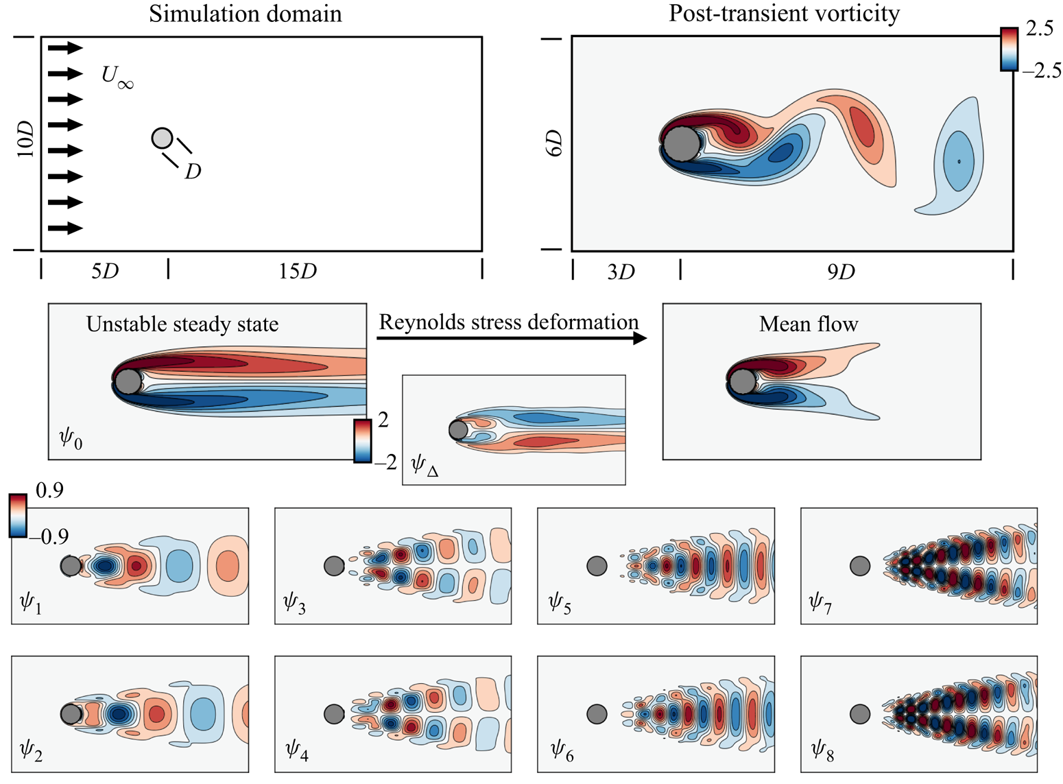
Figure 3. Vortex shedding in the wake of a circular cylinder at  $Re = 100$. En route to the periodic post-transient flow, Reynolds stresses deform the background flow from the unstable steady state to the marginally stable mean flow. This can be approximated in a model by augmenting the POD basis with the ‘shift mode’ $\boldsymbol \psi _\varDelta$. The usual POD modes show the typical structure of spatial and temporal harmonics describing periodically advecting flow features.
The flow regime at Reynolds number 100 is beyond the Hopf bifurcation leading to vortex shedding but below the onset of three-dimensional instability (Noack & Eckelmann Reference Noack and Eckelmann1994; Barkley & Henderson Reference Barkley and Henderson1996; Ma & Karniadakis Reference Ma and Karniadakis2002). The flow is also far enough from the threshold of bifurcation that weakly nonlinear analyses fail to predict the amplitude and frequency of the vortex shedding limit cycle, although a variety of techniques have been used to derive accurate models for the transient and post-transient wake (Noack et al. Reference Noack, Afanasiev, Morzynski, Tadmor and Thiele2003, Reference Noack, Morzynski and Tadmor2011; Manti $\breve{c}$-Lugo et al. Reference Mantic-Lugo, Arratia and Gallaire2014; Loiseau & Brunton Reference Loiseau and Brunton2018; Loiseau et al. Reference Loiseau, Noack and Brunton2018b).
Following Noack et al. (Reference Noack, Afanasiev, Morzynski, Tadmor and Thiele2003) and Loiseau et al. (Reference Loiseau, Brunton and Noack2018a), we compute POD modes from 100 snapshots of the mean-subtracted velocity field, equally spaced over one period of vortex shedding; the pressure gradient term can be shown to be negligible for Galerkin models of this flow. In order to construct a basis that can span the deformation between the unstable steady state and mean flow, we augment the POD basis with the ‘shift mode’, visualized in figure 3. This additional mode is computed from the difference between the base and mean flows and then orthonormalized with respect to the rest of the POD modes with the Gram-Schmidt process. We denote the coefficient of this mode by  $a_\varDelta (t)$ to distinguish it from the usual POD modes.
The full expansion basis then consists of eight POD modes capturing the limit-cycle vortex shedding, plus the shift mode. We take the unstable steady state to be the base flow of the modal expansion so that the origin is a fixed point of the POD–Galerkin system. This basis accurately represents the kinematics of the post-transient flow, with a normalized energy residual of  ${O}(10^{-4})$ (Loiseau et al. Reference Loiseau, Brunton and Noack2018a).
5.2. Lid-driven cavity flow
Lid-driven cavity flow is another idealized geometry that serves as a benchmark problem for numerical methods and model reduction (Arbabi & Mezić Reference Arbabi and Mezić2017; Arbabi & Sapsis Reference Arbabi and Sapsis2022; Lee, Dowell & Balajewicz Reference Lee, Dowell and Balajewicz2019; Rubini, Lasagna & Ronch Reference Rubini, Lasagna and Ronch2020). The flow, shown in figure 4, takes place on a square domain with  $(x, y) \in (-L, L) \times (-L, L)$ with $L=1$. A velocity profile is imposed on the upper boundary, given by
 \begin{equation} u(x, L) = U(1 - x^2)^2. \end{equation}
This driving velocity profile roughly approximates the shear-driven flow over an open cavity at a much lower computational cost, although the dynamics of the shear- and lid-driven cavities is different. The regularized fourth-order velocity profile on the lid avoids numerical problems where the lid meets the no-slip boundaries on the other walls.
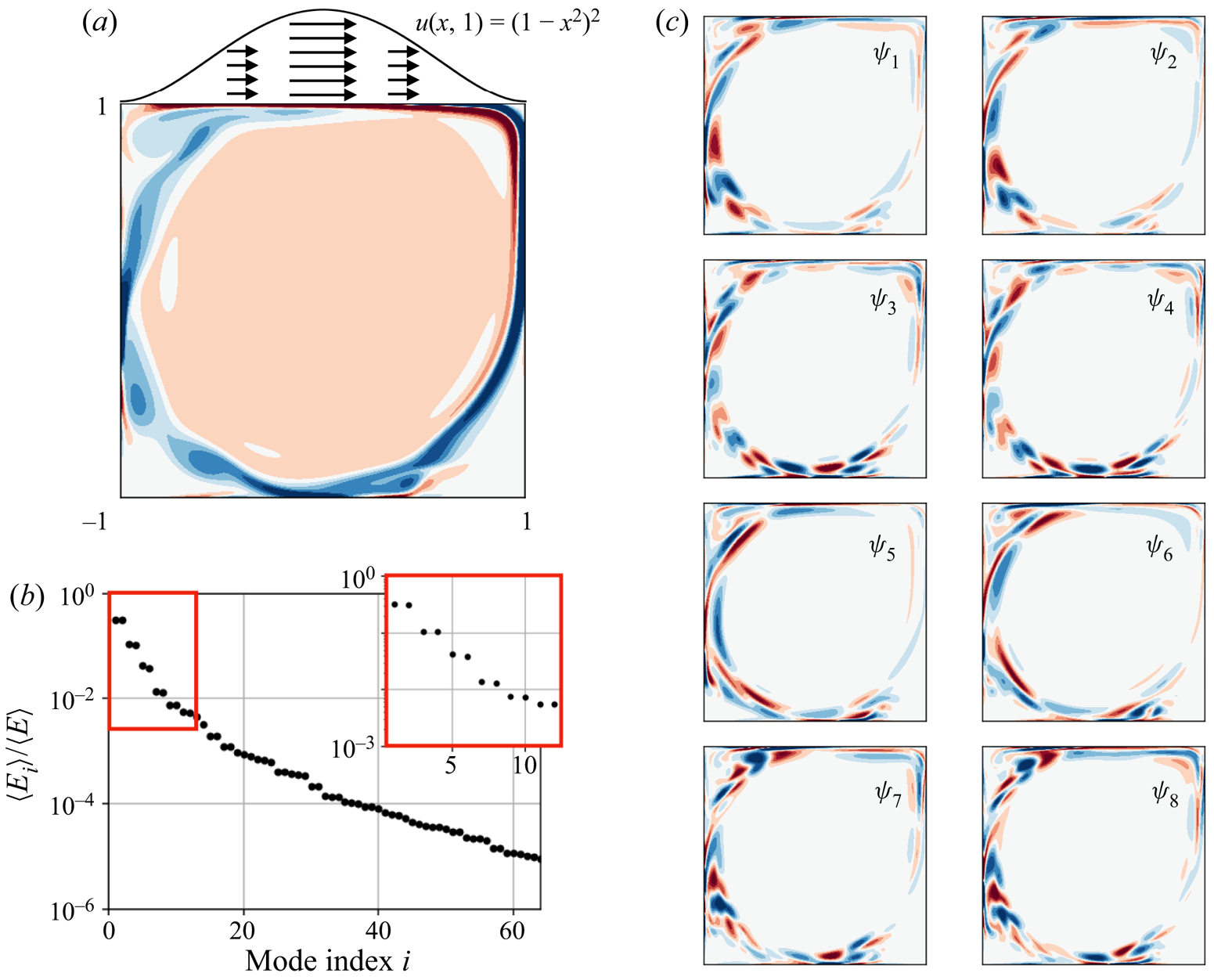
Figure 4. Regularized lid-driven cavity flow at  $Re = 20\,000$. The singular value spectrum is slow to converge (a,b), indicating that relatively many modes are necessary for an accurate kinematic approximation. The leading POD modes themselves appear roughly in pairs with similar spatial structure and frequency content (c). As for the cylinder wake shown in figure 3, this usually indicates oscillatory dynamics, although the evolution of the temporal coefficients is much more irregular in this chaotic flow than for the periodic wake.
The standard Reynolds number for this flow is defined as  $Re = UL/\nu$ based on the cavity half-height and forcing velocity. The flow follows the stereotypical Ruelle–Takens route to chaos parameterized by Reynolds number, undergoing a Hopf bifurcation at $Re_c^{(2)} \approx 10\,250$, a secondary Hopf bifurcation to quasiperiodic flow at $Re_c^{(2)} \approx 15\,500$, and a final bifurcation to chaos near $Re_c^{(3)} \approx 18\,000$ (Lee et al. Reference Lee, Dowell and Balajewicz2019). We simulate the flow in the chaotic regime at $Re = 20\,000$.
The numerical configuration is similar to that described by Arbabi & Sapsis (Reference Arbabi and Sapsis2022). The domain is discretized with 50 seventh-order spectral elements in each direction, refined towards the walls. The flow is integrated for 3000 time units, saving snapshots at a sampling rate  ${\rm \Delta} t = 0.1$. Again, the pressure gradient term vanishes for this closed flow (Noack et al. Reference Noack, Papas and Monkewitz2005), so the velocity POD modes are computed from the first 5000 snapshots, with the remaining 25000 snapshots retained for the statistical comparison in § 6.2. Figure 4 shows a snapshot of the DNS along with the leading POD modes and the singular value spectrum.
5.3. Incompressible mixing layer
As a more difficult test of the proposed MMR closure method, we also examine models of an incompressible mixing layer, pictured in figure 11. The mixing layer is a canonical example of a free shear flow exhibiting convective instability (Monkewitz & Huerre Reference Monkewitz and Huerre1982; Huerre & Monkewitz Reference Huerre and Monkewitz1985, Reference Huerre and Monkewitz1990). Inlet forcing is used to excite Kelvin–Helmholtz instability waves, which roll up into approximately discrete vortices. These vortices are subject to a secondary instability (Brancher & Chomaz Reference Brancher and Chomaz1997) and undergo successive helical pairing at the subharmonic of the primary Kelvin–Helmholtz frequency, a process that drives the linear growth of the mixing layer (Winant & Browand Reference Winant and Browand1974). At higher Reynolds numbers and in three dimensions, the turbulent mixing layer is dominated by the linear growth of coherent structures similar to those seen in two-dimensional simulation (Brown & Roshko Reference Brown and Roshko1974; Stanley & Sarkar Reference Stanley and Sarkar1997), which play a major role in mixing, transport and entrainment of the turbulent flow (Hussain Reference Hussain1981). From a global perspective, the flow behaves as an amplifier, where strong non-normality in the linear operator results in transient algebraic energy growth of small perturbations (Chomaz Reference Chomaz2005).
By analogy to numerical methods, modelling an advection-dominated flow with a POD–Galerkin approach is generally ill advised in much the same way that pseudospectral methods are not ideal for solving hyperbolic (advection) equations. Although the vortices shed in the flow past a cylinder are also travelling waves in a sense, the Kelvin–Helmholtz instability in the mixing layer is convective in nature in contrast with the absolute instability in the cylinder wake. For these reasons, Galerkin projection onto a global modal basis such as POD is not a natural way to approximate shear flows like the mixing layer. Nevertheless, both free and wall-bounded shear layers are present in a wide variety of flows, so in order to employ a low-dimensional dynamical systems model it is important that it be able to capture these features. The challenge of modelling advection-driven phenomena in a global reduced-order modelling framework motivates the use of similar configurations in several studies of stabilization methods for Galerkin-type systems (Ukeiley et al. Reference Ukeiley, Cordier, Manceau, Delville, Glauser and Bonnet2001; Noack et al. Reference Noack, Papas and Monkewitz2005; Balajewicz, Dowell & Noack Reference Balajewicz, Dowell and Noack2013; Cordier et al. Reference Cordier, Noack, Tissot, Lehnasch, Delville, Balajewicz, Daviller and Niven2013).
Since the flow becomes increasingly complex downstream, the difficulty of modelling the flow can be tuned by varying the streamwise extent of the domain. In contrast, the observed dynamics of the cylinder wake and lid-driven cavity is not strongly dependent on domain extent. We construct models on both short ( $L_x = 150$) and long ( $L_x = 250$) domains, as shown in figure 5. Over the extent of the short domain, the flow is mainly characterized by the initial instability and vortex rollup, with the earliest signs of vortex pairing at $x \gtrsim 130$. On the full domain, the vortex pairing accounts for a much larger fraction of the fluctuation kinetic energy, as shown by the POD analysis below.

Figure 5. Proper orthogonal decomposition applied to the mixing layer. The primary shear layer instability forms Kelvin–Helmholtz waves that roll up into vortices, which in turn undergo successive vortex pairing (a). Modes computed on both the short and long domains (c) reveal modes related to the dominant flow features: the shear layer instability and the downstream vortex pairing. Although the vortex pairing is secondary to the upstream instability, on the longer domain it accounts for a larger proportion of the fluctuation kinetic energy (b). Higher-order modes not pictured here include harmonics, nonlinear cross-talk and modes related to irregularity in the location of the vortex pairing events.
The inlet profile is a standard hyperbolic tangent
 \begin{equation} U(y) = \bar{U} + ({\rm \Delta} U / 2 ) \tanh 2y, \end{equation}
where  $\bar {U} = (U_1 + U_2)/2 \equiv 1$ and ${\rm \Delta} U = U_1 - U_2$ in terms of the free-stream velocities $U_1$ and $U_2$ above and below the layer, respectively, and the length scale is non-dimensionalized by the initial vorticity thickness $\delta _\omega = {{\rm \Delta} U}/{U'(0)}$. We define a Reynolds number $Re = \delta _\omega (0) {\rm \Delta} U / \nu$ based on initial vorticity thickness, velocity difference ${\rm \Delta} U$ across the layer and kinematic viscosity $\nu$ and set $Re = 500$ in the simulation. The domain consists of 5200 eleventh-order spectral elements on $x, y \in (-10, 300) \times (-50, 50)$, but the full streamwise extent is masked to $x, y \in (0, 250) \times (-20, 20)$ for modelling in order to discount any boundary effects. The domain is shown in figure 11.
This configuration roughly follows that described by Balajewicz et al. (Reference Balajewicz, Dowell and Noack2013) and Cordier et al. (Reference Cordier, Noack, Tissot, Lehnasch, Delville, Balajewicz, Daviller and Niven2013), with two key differences. First, we simulate incompressible flow, while these authors simulate isothermal compressible flow at low Mach numbers ( $Ma \sim 0.1$). Consequently, we replace the ‘sponge’ boundary conditions for far-field acoustic waves with a region of increased viscous damping corresponding to $Re = 50$ for $x > 250$ to avoid numerical instability at the outflow. Second, rather than disturbing the inlet with random solenoidal perturbations, we use eigenfunction forcing described in Appendix A, similar to that employed by Colonius, Lele & Moin (Reference Colonius, Lele and Moin1997).
The DNS is run until a final time of  $t=2820$, corresponding to fifty periods of the lowest-frequency component of the eigenfunction forcing, saving at every tenth time step with ${\rm \Delta} t = 0.00705$. The POD modes are then computed from the first 10 % of these snapshots (4000 fields), with the remainder reserved for statistical comparison with the models. The domain truncation can be accomplished by simply setting elements of the weight matrix $\boldsymbol{\mathsf{W}}$ in (2) to zero for mesh locations with $x > L_x$ so that these locations do not contribute to the statistics in the correlation matrix. For the mixing layer we compute modes with both velocity and pressure fields, as described in § 2, since the pressure gradient term is not necessarily negligible in Galerkin models of free shear flows (Noack et al. Reference Noack, Papas and Monkewitz2005).
Figure 5 shows the leading POD eigenvalues and modes for both domains. In both cases the bulk of the fluctuation kinetic energy is contained in the first four modes, with the remainder of the spectrum decaying relatively slowly. As expected, the dominant mode pair for the shorter domain corresponds to the Kelvin–Helmholtz waves, while the second pair represents the onset of vortex pairing at roughly half the spatial wavenumber. Higher-order modes are either harmonics (such as the third mode pair) or less regular downstream structures related to slight variations in the vortex pairing.
The directed graph of energy transfers in figure 1 is constructed from the modes computed on the short domain. Specifically, the leading mode pair and its first three harmonics are shown for a simple visualization of the energy cascade; the nodes labelled  $a_1$– $a_8$ thus actually correspond to mode pairs $(\boldsymbol \varphi _1, \boldsymbol \varphi _2)$, $(\boldsymbol \varphi _5, \boldsymbol \varphi _6)$, $(\boldsymbol \varphi _{17}, \boldsymbol \varphi _{18})$ and $(\boldsymbol \varphi _{24}, \boldsymbol \varphi _{25})$. The thickness of the edge from node $a_i$ to $a_j$ is proportional to $\sum _{k} Q_{ijk} \overline {a_i a_j a_k}$ for the quadratic Galerkin tensor $\boldsymbol{\mathsf{Q}}$, which is roughly related to average nonlinear energy transfer from one mode to the other, although it should not necessarily be interpreted in any rigorous way beyond the purposes of conceptual visualization of the energy cascade.
On the longer domain the vortex pairing makes up a larger proportion of the fluctuation kinetic energy. Consequently, the leading four modes are spatially localized downstream, representing vortex pairing, while the upstream linear instability is not evident until the third mode pair, even though the vortex pairing is secondary to the shear layer instability from a physical perspective.
The slowly decaying POD spectrum and wave-like spatial structure of the modes are a consequence of the advection-driven nature of this flow. It is well known that the space–time separation of variables assumed by POD is not a natural representation of travelling waves. This is one reason that free shear flows have long posed difficulties for POD–Galerkin modelling, making this a challenging test case for the MMR approach.
6. Results
In this section we evaluate the proposed MMR closure method on several numerical test problems. In § 6.1 we analyse vortex shedding behind a circular cylinder, showing that the method reproduces the classic invariant manifold model due to Noack et al. (Reference Noack, Afanasiev, Morzynski, Tadmor and Thiele2003), which must account for both mean-flow deformation and the energy cascade in order to accurately model the transient dynamics. As a more challenging test in § 6.2, we show that the multiscale closure stabilizes a reduced-order model of the chaotic lid-driven cavity flow, while closely matching the spectral energy content of the DNS. Finally, in § 6.3 we develop a model for convective instability and subharmonic vortex pairing in the spatially evolving mixing layer.
By means of these examples, we show that the proposed approach for multiscale closure is a systematic method for eliminating degrees of freedom from reduced-order models that can resolve critical subscale phenomena and produce stable models of dynamically complex unsteady flows. More broadly, the multiscale framework represents a general description of the means by which effective cubic nonlinearity arises in low-dimensional models.
As a general comment on the following figures, in order to evaluate the quality of the dynamical approximation (rather than that of detailed time-series forecasts) we choose visualizations that capture the overall statistical behaviour of the system more broadly than time series. In particular, we focus on fluctuation energy levels, estimated power spectral densities and phase portraits, which may be interpreted as approximate slices of joint probability distributions. However, for the sake of completeness we provide a comparison of forecasting errors in Appendix C.
6.1. Vortex shedding in the cylinder wake
In this section we revisit the canonical two-dimensional flow past a circular cylinder to show that the MMR closure can naturally resolve the stabilizing effects, both of mean-flow deformation and of energy transfer to higher-order modes, without assuming proximity to a bifurcation.
In keeping with previous work demonstrating that the cylinder wake can be modelled accurately with as few as two degrees of freedom, we reduce the 9-mode POD–Galerkin system to a 2-mode generalized Stuart–Landau model (4.18b) with the closure model (4.19) and damping derived from the energy-balance relation (4.20). The first 9 modes capture >99.9 % of fluctuation kinetic energy for this flow. In this case, the elimination of the higher-order modes does not require sacrificing kinematic resolution, since the unresolved coefficients can be approximated as sparse polynomial functions of the resolved variables (Loiseau et al. Reference Loiseau, Brunton and Noack2018a; Callaham et al. Reference Callaham, Brunton and Loiseau2022).
Figure 6(a) compares the energy of the first mode pair,  $E(t) = a_1^2(t) + a_2^2(t)$, predicted by the POD–Galerkin model and the 2-mode closure model, with DNS of the transient flow initialized from the unstable steady state and perturbed by the least-stable eigenmode. Also included for comparison is the invariant manifold model introduced by Noack et al. (Reference Noack, Afanasiev, Morzynski, Tadmor and Thiele2003). Although the Galerkin model is stable and accurately predicts the amplitude of the vortex shedding, it exhibits a transient energy overshoot before settling onto the limit cycle. Figure 6(b) shows the reason for this; whereas the DNS is restricted to an approximately parabolic invariant manifold, the finite relaxation time in the shift mode dynamics results in the energy of the leading modes continuing its exponential growth for longer before the energy can be absorbed into the mean-flow deformation.

Figure 6. Reduced-order models of the cylinder wake. The standard 9-mode Galerkin model accurately estimates the stable limit cycle (a), but the transient dynamics deviates from the slow manifold, leading to an energy overshoot (b). Both the two-dimensional invariant manifold reduction (Noack et al. Reference Noack, Afanasiev, Morzynski, Tadmor and Thiele2003) and MMR closure models prevent this by eliminating the rapidly equilibrating variable associated with mean-flow deformation, but MMR more accurately estimates the limit-cycle amplitude. The full flow field can be reconstructed by approximating the harmonics with polynomial regression (c).
In contrast, the cubic term in the MMR and invariant manifold models approximates the relaxation of the shift mode dynamics as instantaneous, pinning its amplitude to that of the primary mode pair. While the structure and interpretation of the two models is the same, there are quantitative differences in their accuracy. In particular, the manifold model slightly overestimates the energy of the limit cycle, with mode amplitudes larger than the DNS by  $\sim$13 %, while the multiscale closure accurately predicts the limit-cycle amplitude. This discrepancy can most likely be attributed to the energy-balance procedure used to estimate the subscale damping $\boldsymbol \nu$ in the MMR model, which is not used in the invariant manifold model.
Finally, the full flow field can also be reconstructed from the two-degree-of-freedom multiscale model by means of the sparse polynomial approximation to the nonlinear correlations in the higher-order modes (figure 6c). The flow field predicted by the model gives a good approximation of the DNS solution, although over long times the phase of the vortex shedding tends to drift from that of the high-dimensional solution. By systematically averaging over the fast variables, the multiscale closure method is thus able to reduce the dimensionality of the model while also improving its fidelity.
6.2. Chaotic lid-driven cavity flow
The Stuart–Landau equation derived for the cylinder wake in § 6.1 is an example of a relatively simple nonlinear oscillator with either a stable fixed point or periodic limit cycle as an equilibrium. Here, we show that the MMR closure approach can also be applied to systems with a more complex dynamics, as illustrated on the chaotic lid-driven cavity flow introduced in § 5.2.
First, we construct a standard POD–Galerkin model with  $r=64$ modes, sufficient to capture ${\sim }99.8\,\%$ of the fluctuation kinetic energy. The Galerkin system is chaotic and energetically stable. Despite its precise kinematic resolution, the Galerkin model is inaccurate, overestimating the kinetic energy by roughly one order of magnitude, as shown by the blue traces in figure 7.
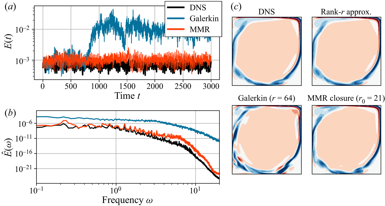
Figure 7. Reduced-order models of the lid-driven cavity flow. The Galerkin system eventually equilibrates at much higher energy levels, while the MMR closure model produces stable predictions that closely match the power spectrum of the chaotic flow (a,b). The reconstructed fields from the MMR model are also more physically consistent with the DNS than the Galerkin model (c). For comparison, the top right panel shows the reconstruction of the DNS flow field using an equal number of modes as the POD–Galerkin system ( $r=64$).
Reducing the model to  $r_0 = 21$ degrees of freedom via a multiscale closure stabilizes it with an equilibrium energy that approximately matches the power spectrum of the DNS (figure 7, orange). The MMR model still retains enough modes for a ${\sim }98\,\%$ accurate POD reconstruction. The predicted flow fields are coherent and qualitatively consistent with the DNS fields, even though they do not match in every detail due to the chaotic nature of the flow.
Varying the dimension  $r_0$ of the approximate slow variables results in models that are energetically stable, but not necessarily chaotic. Instead, many such models eventually settle onto a post-transient dynamics that is periodic or quasi-periodic. The persistence of the dominant frequencies suggests that, even for models with relatively many degrees of freedom ( $r_0>2$), the generalized Stuart–Landau equations produced by the MMR closure scheme can be viewed as coupled nonlinear oscillators, especially when the spatial components of the POD modes suggest that they may be grouped in pairs with similar temporal frequency content.
6.3. Convective instability and vortex pairing in a mixing layer
Advection-dominated flows have historically posed a challenge for reduced-order models, primarily because the global mode ansatz of POD is a poor representation of travelling waves. As a final numerical example, we apply the MMR closure to model the mixing layer introduced in § 5.3, a canonical example of convective instability in free shear flows.
In one sense, the dynamics of the mixing layer is relatively simple. The flow close to the inlet is dominated by the shear layer instability and subsequent vortex roll-up. These vortices are advected downstream at approximately the midline flow velocity, until the secondary vortex pairing begins at the subharmonic of the primary instability frequency. However, since this behaviour unfolds as the disturbances are carried downstream, a principal challenge for low-dimensional models based on global POD modes is to preserve phase coherence between the harmonics and subharmonics, so that the reconstructed flow fields consist of approximately discrete vortices undergoing the vortex pairing.
As discussed in § 5.3, both the POD mode basis and the difficulty of modelling this flow depend on the streamwise extent of the domain. Since the subharmonic vortex pairing is energetically dominant downstream, the leading POD modes computed from a longer domain will be related to vortex pairing, even though the primary shear layer instability drives the dynamics from a physically causal perspective. To illustrate this effect, we consider two domain lengths: one that is dominated by the primary instability and vortex roll-up, and the full modelling domain with vortex pairing.
In this case the POD–Galerkin models do not necessarily improve with an increasing number of modes. For both domains, the best dynamical approximation is found for models constructed from  $r=24$ modes, corresponding to 99.8 % of fluctuation kinetic energy on the short domain and 98.4 % on the long domain. On the short domain ( $L_x = 150$), this model is energetically stable but eventually approaches an unphysical fixed point (figure 8). On the longer domain ( $L_x = 250$), the model initially follows the DNS trajectory before eventually becoming unstable (figure 9). In either case, increasing the dimension of the POD–Galerkin model resulted in worse models. We then reduce the $24$-dimensional Galerkin systems to $r_0=16$-dimensional generalized Stuart–Landau models with the MMR closure.

Figure 8. Models of the mixing layer on a short domain. The phase portraits of the mode pairs (a) show phase locking between the fundamental mode pair  $(a_1, a_2)$, the subharmonic vortex pairing $(a_3, a_4)$, and the first harmonic $(a_5, a_6)$. These phase relationships are preserved by the MMR closure, resulting in physically consistent flow field estimates (b–d).
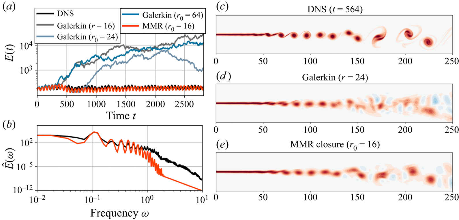
Figure 9. Mixing layer models on the long domain. While standard POD–Galerkin models are energetically unstable until at least  $r=64$, the multiscale closure stabilizes the model with only 16 variables (a,b). The model also remains coherent on long integration times (see also figure 10), producing flow field predictions that are consistent with the large-scale structure of the DNS (c–e).

Figure 10. Phase portraits of the mixing layer model on the long domain. The MMR closure (orange) closely matches the DNS trajectories (black) for the most energetic modes, even though the structure is more complicated than the Lissajous-type harmonics on the short domain (figure 8). This figure does not show a Galerkin model for comparison because they are energetically unstable (figure 9).
Figure 8 shows the comparison of the closed model with the DNS and Galerkin systems for the short domain. The MMR model closely matches the phase portraits of the DNS, indicating that it preserves the phase relationships between the various modes, including the early subharmonic vortex pairing  $(a_3, a_4)$ and higher harmonics, e.g. $(a_5, a_6)$. This remains true even when integrated to very long times (the final integration time is $t=2820$ in this case, as with the DNS described in § 5.3). As a result, the approximated fields are highly coherent, with the same pattern of vortex roll-up, advection, and pairing as seen in the DNS (figure 8b–d).
On the longer domain, the multiscale closure also stabilizes the Galerkin model. Figure 9 compares the true energy content of the POD coefficients with that predicted by the model, both in the time and frequency domain. Although the evolution of the energy matches at the dominant frequencies, the MMR model does not capture the weakly chaotic dynamics exhibited by the DNS as a result of slight irregularity in the vortex pairing. Instead, after a brief transient the solution becomes approximately periodic with phase locking between the modes (figure 10). As with the short domain, this synchronization ensures that the predicted flow fields remain coherent, even when integrated for long times (figure 9c–e).
As might be anticipated based on the more complex dynamics on the longer domain, the fields predicted by the MMR model do not match the DNS quite as closely as on the shorter domain, particularly closer to the inlet. This is likely because fine-scale resolution of the upstream region of the flow requires higher harmonics of the primary instability that do not appear in the POD modes of the longer domain until much higher-order mode number. Higher-resolution predictions might therefore be constructed by applying nonlinear correlations analysis and polynomial regression to selected higher-order modes, as in the cylinder reconstruction in § 6.1; see also Loiseau et al. (Reference Loiseau, Brunton and Noack2018a) and Callaham et al. (Reference Callaham, Brunton and Loiseau2022). Still, the dominant vortices are still evident in the prediction of the low-dimensional model, even in the downstream pairing region.
On both domains, the synchronization and long-time phase coherence between the modes further reinforces the picture outlined in § 6.2 of the closure model as consisting of coupled nonlinear oscillators. Although the description of this flow in terms of spatially fixed global modes is not an ideal representation of the advection-driven dynamics, the proposed MMR closure method is able to successfully stabilize the POD–Galerkin models and accurately capture the phase relationships necessary for accurate predictions of the full flow fields.
7. Conclusion
In this work, we have developed a MMR approach to improving linear–quadratic dynamical systems derived from POD–Galerkin projection of the Navier–Stokes equations, with the addition of systematically computed cubic closure terms. These cubic closure terms are derived through an adaptation and application of a multiscale stochastic averaging method that originated in singular perturbation theories of Markov processes (Kurtz Reference Kurtz1973; Papanicolaou Reference Papanicolaou1976; Majda et al. Reference Majda, Timofeyev and Vanden-Eijnden2001; Weinan Reference Weinan2011; Pavliotis & Stuart Reference Pavliotis and Stuart2012). Whereas the standard truncation of the Galerkin system disregards the influence of unresolved variables, the proposed MMR method accounts for their effect through averaging via a stochastic Koopman operator. In particular, this approach is able to model nonlinear interactions between resolved and unresolved variables, capturing key mechanisms such as mean-flow deformation and the energy cascade. The closed model includes cubic terms, taking the form of generalized Stuart–Landau equations that often act as coupled nonlinear oscillators.
Since the derivation of the MMR closure method relies on an asymptotic time-scale separation between resolved and subscale variables that is generally absent in fluid flows, we have not attempted to prove the general validity of this approach when the flow is not close to a bifurcation. Instead, we demonstrated by numerical example that the method dramatically improves the stability and accuracy of low-dimensional models of unsteady fluid flows compared with the standard POD–Galerkin models. After a comparison with the well-known benchmark problem of vortex shedding in a cylinder wake, we have shown that the MMR method can reproduce the chaotic dynamics in lid-driven cavity flow. Finally, we developed models of an incompressible mixing layer and showed that the coupled-oscillator MMR closures not only stabilize the models, but preserve phase relationships between the modes, which is critical for physically consistent predictions of advection-driven flow.
These results raise several possibilities for interesting future work. For example, the mixing layer is an ‘amplifier’ flow characterized by convective instability and transient energy growth. It is therefore highly sensitive to the nature of the upstream flow; models developed for a specific inlet forcing may not generalize. Further consideration of this issue could be the foundation of a multiscale approach to input/output models in the resolvent framework (McKeon & Sharma Reference McKeon and Sharma2010; Sharma & McKeon Reference Sharma and McKeon2013; Zare, Jovanović & Georgiou Reference Zare, Jovanović and Georgiou2017; Padovan et al. Reference Padovan, Otto and Rowley2020; Pickering et al. Reference Pickering, Rigas, Schmidt, Sipp and Colonius2021). In this work we neglect the time-varying boundary condition in the region upstream of the modelling domain, but an input/output model could more properly treat this explicitly as forcing, as is done for instance in control-oriented reduced-order models (Barbagallo, Sipp & Schmid Reference Barbagallo, Sipp and Schmid2009; Sipp et al. Reference Sipp, Marquet, Meliga and Barbagallo2010). Recent work on trajectory-based optimal oblique projections has also shown promise for capturing dynamically important, but typically low-energy, modes in an input–output framework for model reduction of open shear flows (Otto, Padovan & Rowley Reference Otto, Padovan and Rowley2022).
Amplifier flows are therefore one potential failure mode for the MMR method as presented here. This may be understood as a reflection of the unsuitability of standard POD–Galerkin for input–output modelling. By extension, without further development MMR would also most likely struggle to model configurations with time-varying base flows or actuation. As a more fundamental limitation, this approach does depends on the presumption of underlying low-dimensional structure in the dynamics of the flow. As a limiting case, MMR would likely fail to produce useful models of homogeneous isotropic turbulence.
As discussed for the chaotic lid-driven cavity flow in § 6.2, we have observed that the MMR models often tend towards phased-locked periodic or quasiperiodic solutions rather than chaos, consistent with the idea of a system of weakly coupled oscillators. However, we expect that in the development of models of chaotic or turbulent flows it may be helpful to re-introduce some degree of stochasticity to better match the flow statistics. Fortunately, this is straightforward in the multiscale modelling framework (Weinan Reference Weinan2011; Pavliotis & Stuart Reference Pavliotis and Stuart2012). For instance, the homogenization method (Majda et al. Reference Majda, Timofeyev and Vanden-Eijnden2001) begins from slightly different scaling assumptions and results in a closed model in which the fast-scale stochastic forcing appears as a new diffusion term. A careful investigation of different scale separation assumptions and stochastic approximations could be valuable in extending this framework to turbulent flows. The diagonal drift approximation could also be revisited; numerical estimation of the ‘stationary’ distribution of the fast Ornstein–Uhlenbeck process by solving the Lyapunov equation at each time step may improve the accuracy of averaging enough to justify the additional computational cost.
Moreover, since successful POD–Galerkin models of chaotic or turbulent flows often depend on explicit models of mean-flow deformation (Aubry et al. Reference Aubry, Holmes, Lumley and Stone1988; Ukeiley et al. Reference Ukeiley, Cordier, Manceau, Delville, Glauser and Bonnet2001) or subscale dissipation (Rempfer & Fasel Reference Rempfer and Fasel1994; Noack et al. Reference Noack, Schlegel, Ahlborn, Mutschke, Morzynski, Comte and Tadmor2008; Wang et al. Reference Wang, Akhtar, Borggard and Iliescu2012; Cordier et al. Reference Cordier, Noack, Tissot, Lehnasch, Delville, Balajewicz, Daviller and Niven2013; Östh et al. Reference Östh, Noack, Krajnovic̀, Barros and Borèe2014), both of which can be approximated naturally in the multiscale modelling framework, the MMR approach may be useful as a general approach to subscale and mean-flow modelling that is independent of the flow geometry.
The potential application to flows with continuous spectral components still relies conceptually on the existence of low-dimensional structure in the flow, although the success of filtering in flows with broadband turbulence to perform large-eddy simulation (LES) raises the possibility of a subscale LES-type closure model based on multiscale analysis. This might take the form of a multiple-scale expansion in both space and time or of a filter designed for the isotropic scales of turbulence, for instance. In either case, the Stuart–Landau form of the MMR closure model suggests that a spatio-temporal analysis would be akin to a Ginzburg–Landau theory of turbulence modelling.
In this work we have only considered a linear–quadratic dynamics derived from POD–Galerkin projection. This has the advantage of being based on the governing equations, but recent work has shown that data-driven model discovery can be a powerful alternative (Brunton et al. Reference Brunton, Proctor and Kutz2016; Loiseau & Brunton Reference Loiseau and Brunton2018; Loiseau et al. Reference Loiseau, Brunton and Noack2018a,Reference Loiseau, Noack and Bruntonb; Deng et al. Reference Deng, Noack, Morzynski and Pastur2020; Qian et al. Reference Qian, Kramer, Peherstorfer and Willcox2020; Rubini et al. Reference Rubini, Lasagna and Ronch2020; Callaham et al. Reference Callaham, Brunton and Loiseau2022). Data-driven modelling is especially useful when the governing equations are unknown or projection-based modelling is not as straightforward, as for incompressible fluid flow (Loiseau Reference Loiseau2020; Qian et al. Reference Qian, Kramer, Peherstorfer and Willcox2020; Guan, Brunton & Novosselov Reference Guan, Brunton and Novosselov2021). In a sense, data-driven modelling might circumvent the need for closure modelling by fitting directly to the time series, including leveraging the intuition that cubic terms will appear in the effective dynamics (Loiseau & Brunton Reference Loiseau and Brunton2018). However, the linear–quadratic system has certain symmetries and conservation properties that can be enforced in constrained regression to a quadratic model (Schlegel & Noack Reference Schlegel and Noack2015; Loiseau & Brunton Reference Loiseau and Brunton2018; Kaptanoglu et al. Reference Kaptanoglu, Callaham, Hansen, Aravkin and Brunton2021a,Reference Kaptanoglu, Morgan, Hansen and Bruntonb), while extending these properties to cubic nonlinearity is not straightforward. An interesting future direction could be exploring a two-step process, first identifying a quadratic model that satisfies the constraints, and then applying the MMR closure to reduce it to a lower-dimensional cubic model. Since the empirical models are often sparse, this could potentially result in models with improved stability and scaling compared with the projection-based approach. Alternatively, a more flexible deep-learning model could be used to replace the proposed diagonal drift approximation, for instance with a modified variational autoencoder (Kingma & Welling Reference Kingma and Welling2013) that parameterizes the distribution of subscale variables conditioned on the slow variables.
It will also be interesting to extend this analysis to systems where the leading-order cubic terms tend to destabilize the system, such as the subcritical bifurcation in plane Poiseuille flow (Stewartson & Stuart Reference Stewartson and Stuart1971). This is an important scenario in the transition to turbulence, particularly for shear flows in which non-normal energy amplification can activate the nonlinearity even when the flow is globally stable. Higher-order effective nonlinearity could potentially be incorporated into the framework via state-dependent diffusion or an alternative fast drift model, for instance.
Beyond the context of POD–Galerkin reduced-order modelling, the MMR framework represents a general theory of effective cubic nonlinearity arising in amplitude equations for global modes in quadratically nonlinear fluid flow. The system of generalized Stuart–Landau equations produced by the closure model presents a picture of the flow as a set of coupled nonlinear oscillators describing the evolution of mode pairs. Close to the threshold of instability the MMR closure is consistent with a weakly nonlinear analysis, but it does not rely on proximity to a bifurcation. The multiscale modelling methodology is therefore an alternative to standard asymptotic expansions that may have implications for a variety of theoretical and numerical approaches to modelling the large, slow scales of unsteady fluid flows.
Funding
S.L.B. acknowledges funding support from the Army Research Office (ARO W911NF-19-1-0045), the Air Force Office of Scientific Research (AFOSR FA9550-21-1-0178) and National Science Foundation AI Institute in Dynamic Systems (grant number 2112085). J.L.C. acknowledges funding support from the Department of Defense (DoD) through the National Defense Science & Engineering Graduate (NDSEG) Fellowship Program.
Declaration of interests
The authors report no conflict of interest.
Appendix A. Stability analysis of the mixing layer inlet profile
This appendix describes the eigenfunction forcing applied at the inlet of the mixing layer configuration described in § 5.3. The flow acts an amplifier (Huerre & Monkewitz Reference Huerre and Monkewitz1985, Reference Huerre and Monkewitz1990; Chomaz Reference Chomaz2005), so the downstream flow is highly sensitive to the inlet conditions; eigenfunction forcing accentuates the natural dynamics of the flow.
Since the dominant Kelvin–Helmholtz instability is inviscid (Michalke Reference Michalke1964), we derive the forcing from a temporal stability analysis of the inviscid equations linearized about the parallel hyperbolic tangent inlet profile  $\boldsymbol u(\boldsymbol x) = (U(y), 0)$. Defining a perturbation streamfunction $\psi (\boldsymbol x, t)$ with real wavenumber $\alpha$ and complex velocity $c = c_r + \textrm {i} c_i$
 \begin{equation} \psi(\boldsymbol x, t) = \mbox{Re} \left\{ \hat{\psi}(y) \exp({{\rm i}\alpha(x - ct)}) \right\}, \end{equation}
the evolution of the perturbation is given by the Rayleigh equation
 \begin{equation} \left( U - c \right) \left(\frac{{\rm d}^2}{{\rm d}y^2} - \alpha^2 \right) \hat{\psi} - U'' \hat{\psi} = 0. \end{equation}
For each wavenumber  $\alpha$, this can be written as a generalized eigenvalue problem
 \begin{equation} \boldsymbol {\mathcal{A}}(\alpha) \hat{\psi}_j(y; \alpha) = c^{(j)} \boldsymbol{\mathcal{B}}(\alpha) \hat{\psi}_j(y; \alpha), \end{equation}
for the  $j$th velocity $c$ and perturbation streamfunction $\hat {\psi }$, where we use the convention of sorting by decreasing $\mbox {Im}\{c^{(j)}\}$.
The base profile is odd, so the real phase velocity is the midline value  $c_r = \bar {U}$ (Michalke Reference Michalke1964). With $\bar {U} = 1$, perturbations oscillate with frequency $\omega =\alpha$ and growth rate $\sigma (\alpha ) = \alpha c_i(\alpha )$. For further details on linear stability analysis of shear flows, see for example Huerre & Monkewitz (Reference Huerre and Monkewitz1985) and Schmid & Henningson (Reference Schmid and Henningson2012). We choose a spectral discretization of (A2) using a Hermite collocation scheme from a Python implementation of the dmsuite library (Weidemann & Reddy Reference Weidemann and Reddy2000). We find the least stable wavenumber $\alpha ^*$ by maximizing the growth rate $\sigma$ (i.e. minimizing - $\alpha c_i^{(1)}$) using an implementation of the BFGS algorithm available in scipy. Since this departs from the standard shooting method, we validate it against Michalke (Reference Michalke1964), who uses the profile ${U(y) = 0.5( 1 + \tanh y )}$ based on non-dimensionalizing with the shear layer thickness $\delta _\omega /2$ rather than vorticity thickness. With that profile we find a least-stable wavenumber $\alpha ^* = 0.4449$ and growth rate $\sigma = 0.0949$ compared with the reported results of $\alpha ^* = 0.4446$ and $\sigma = 0.0949$. For the present base profile (5.2) we find $\alpha ^* = 0.8912$ and $\sigma = 0.2129$.
Once the wavenumber  $\alpha ^*$ and eigenfunction $\hat {\psi }_1$ corresponding to the maximum growth rate is identified, the inlet velocity perturbation can be computed from
 \begin{equation} \hat{u}_1(y; \alpha^*) = \hat{\psi}_1'(y; \alpha^*),\quad \hat{v}_1(y; \alpha^*) = {\rm i} \alpha^* \hat{\psi}_1(y; \alpha^*) . \end{equation}
The optimal perturbations are shown in figure 11. Following Colonius et al. (Reference Colonius, Lele and Moin1997), we also apply forcing at the first three subharmonics of the least-stable mode computed from solving (A2) at  $\alpha ^*/2$, $\alpha ^*/4$, and $\alpha ^*/8$, rescaling each so that the maximum value of $\hat {u}_1$ is $10^{-3} {\rm \Delta} U$. We perturb the inlet profile by $\mbox {Re}\{ \hat {\boldsymbol u}_1(y, \alpha _n) \exp ({\textrm {i} \omega _n t}) \}$ for $n=1, 2, 4, 8$ and $\alpha _n = \omega _n = \alpha ^*/n$ and use a simulation time step of ${\rm \Delta} t = 0.00705 = 10^{-3} \times 2 {\rm \pi}/ \alpha ^*$, so that the sampling rate of the simulation is commensurate with the forcing frequency.

Figure 11. An incompressible mixing layer at  $Re = 500$. The hyperbolic tangent base flow is convectively unstable, amplifying small perturbations as they are carried downstream. We force the flow at the inlet with eigenfunctions of inviscid flow equations linearized around the base flow (left). The central part of the domain is used for further modelling to avoid boundary effects, while the downstream extent $x \in (250, 300)$ is strongly damped to prevent numerical instability at the outlet.
Appendix B. Variable truncation of the mixing layer model
One of the limitations of projection-based reduced-order modelling for systems without an explicit scale separation is a lack of principled criteria for selecting the truncation rank, or dimension of the projection subspace. A common approach is to use ad hoc criteria such as the number of modes required to resolve some fraction of the fluctuation kinetic energy (e.g. 90 % or 99 %) on average. To some extent this simply replaces the arbitrary choice of rank truncation with an equally arbitrary choice of approximation accuracy. This is especially the case when the dynamic approximation accuracy of the reduced-order model does not monotonically improve with increasing kinematic approximation accuracy (as can be seen in figure 9, for instance).
Unfortunately, this problem is compounded in the secondary reduction step of the MMR method, since one must select both the rank  $r$ of the original POD–Galerkin system and the rank $r_0$ of the final MMR system. Our approach in this work was to follow the heuristic of simulating the POD–Galerkin system at various values of $r$ and choosing that which performs best or remains stable for longest (e.g. $r=24$ for the mixing layer model in figure 9). The final MMR models then typically behave similarly for a range of final ranks $r_0$.
However, in order to show that the method is relatively insensitive to the specific choices of rank truncation, here we repeat the model reduction for the mixing layer on the longest domain shown in figure 9. These models begin with  $r=64$ rather than the ‘optimal’ POD–Galerkin rank of $r=24$. Although less accurate than the model reported in § 6.3, the resulting models are stable for all values $r_0$ of the final rank and significantly outperform any POD–Galerkin model as shown by figure 12.
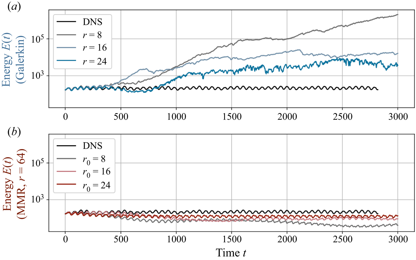
Figure 12. Alternative truncations of the mixing layer model in § 6.3. Rather than the ‘optimal’ value of  $r=24$, the MMR models shown here are constructed from Galerkin systems of rank $r=64$. While the POD–Galerkin models are inaccurate and energetically unstable for any rank truncation, while the MMR models are less sensitive to the specific values of rank truncation.
As a more principled example, figure 13 shows a model constructed by choosing a kinematic reconstruction accuracy threshold of 99 % for the POD–Galerkin rank  $r$. The MMR rank $r_0$ is then selected with the classic ‘elbow’ criterion, which selects a truncation level based on the inflection point of the singular value distribution. Again, the model is less accurate than the results shown in in § 6.3, but significantly more stable and accurate than any Galerkin system. Thus, while a principled approach to rank selection is an open problem for both POD–Galerkin modelling and the proposed multiscale reduction, the latter appears generally less sensitive to this choice.

Figure 13. Truncation of the mixing layer in § 6.3 based on the singular value spectrum. In this case the initial truncation level  $r=32$ is selected based on a residual of 1 %, while the MMR rank $r_0=6$ is based on the ‘knee’ criterion (see text). As with the models shown in figure 12, the resulting model is stable and roughly matches the true dynamics, but is not as accurate as the model reported in § 6.3.
Appendix C. Forecasting accuracy
As discussed in § 6, MMR is not primarily intended to produce accurate forecasts over long time horizons. The underlying POD–Galerkin model is developed based on optimizing the estimate of the instantaneous time derivative, which does not necessarily result in optimal finite-time predictions. Since MMR is developed based on asymptotic consistency with the Galerkin system it is also not optimized for forecasting accuracy. In this, autoregressive methods (Billings Reference Billings2013) that are specifically tailored to forecasting are more appropriate. On the other hand, dynamical accuracy is often more important than long-term forecasting in applications such as the design of feedback controllers (Noack et al. Reference Noack, Morzynski and Tadmor2011; Brunton & Noack Reference Brunton and Noack2015).
However, for the sake of completeness figure 14 gives a comparison of the forecasting accuracy of both the standard POD–Galerkin and MMR models. The error metric is the normalized energy error
 \begin{equation} \frac{{\rm \Delta} E(t)}{E(t)} = \frac{ \|\boldsymbol a_{DNS}(t) - \boldsymbol a_{ROM}(t)\|^2 } {\|\boldsymbol a_{DNS}(t) \|^2 }. \end{equation}
In this metric neither POD–Galerkin nor MMR produces accurate long-term forecasts.
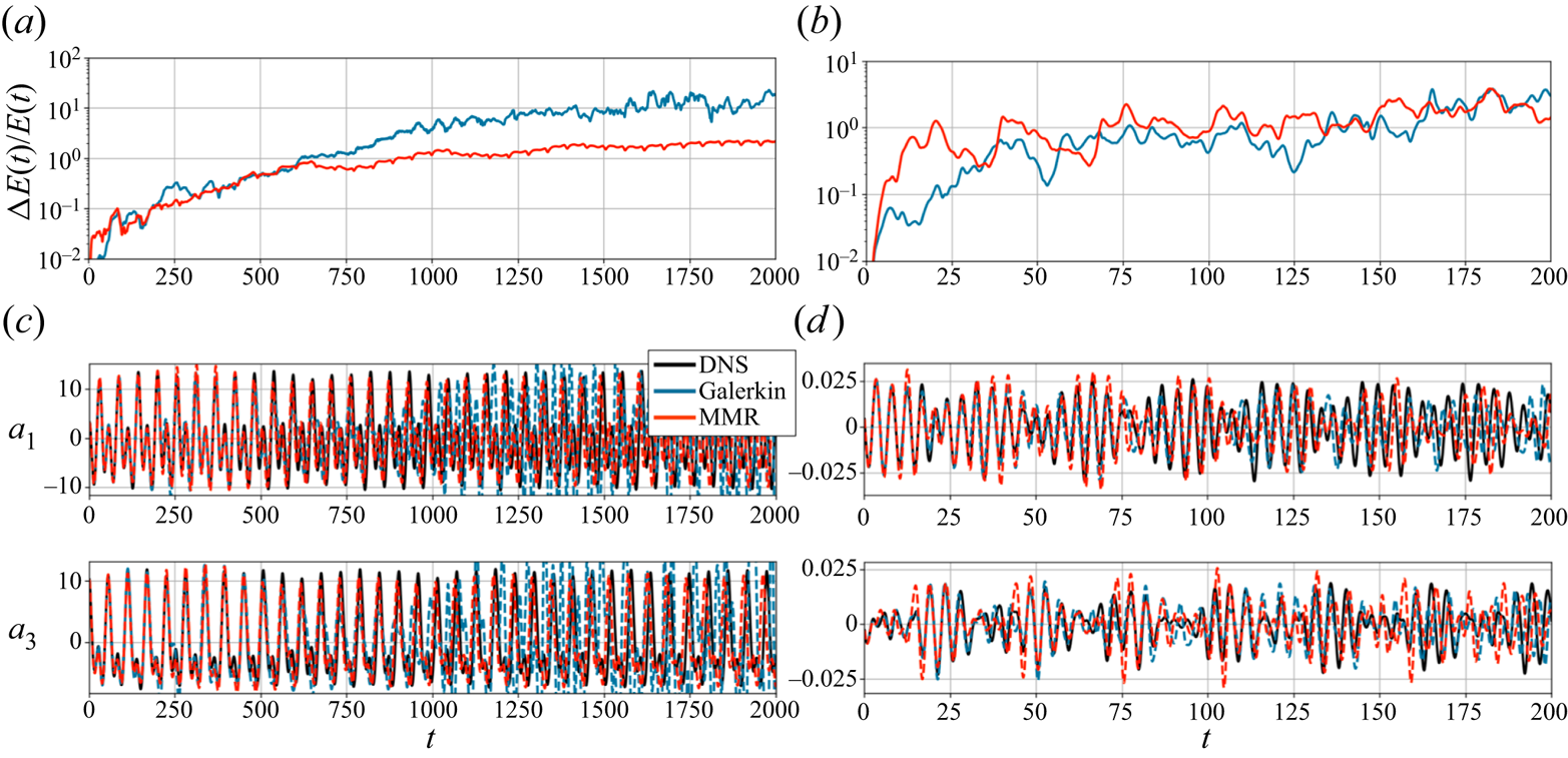
Figure 14. Time-series forecasts for the mixing layer (a,c) and lid-driven cavity (b,d). Due to the complex dynamics of these flows, neither modelling approach produces accurate forecasts over long time horizons. The normalized energy error  ${\rm \Delta} E(t) / E(t)$ is comparable between the standard POD–Galerkin and MMR models (a,b). Predictions for leading individual coefficients show significant errors after several periods of the dominant oscillatory frequency (c,d).
In flows with a relatively simple dynamics (e.g. the cylinder wake or short-domain mixing layer), small errors in the phase of oscillations tend to accumulate over time, even if the dynamical behaviour is modelled accurately. For instance, figure 14(c) shows that errors in MMR-based predictions of individual POD coefficients can largely be attributed to phase drift, while the Galerkin forecast diverges due to dynamical instability.
However, if the flow is chaotic (e.g. the lid-driven cavity) then detailed forecasting on times much longer than that determined by the Lyapunov exponent is impossible even in principle. Hence, while MMR more accurately captures the statistical behaviour of the lid-driven cavity flow (figure 7), it does not improve upon the finite-time predictions of the POD–Galerkin model (figure 14d).


 Open access