


1. Introduction
Two-dimensional internal shear layer structures were reported before in turbulent boundary layers (TBLs) by Meinhart & Adrian (Reference Meinhart and Adrian1995) and Adrian, Meinhart & Tomkins (Reference Adrian, Meinhart and Tomkins2000) as the regions where high gradients in the streamwise velocity occur; and by Eisma et al. (Reference Eisma, Westerweel, Ooms and Elsinga2015) as highly sheared regions. In these studies, it was shown that the shear layers are bounding large-scale energetic motions that have nearly uniform streamwise velocities. Later, several researchers treated the continuous edges of these large-scale motions as shear layers (e.g. Kwon et al. Reference Kwon, Philip, de Silva, Hutchins and Monty2014; de Silva, Hutchins & Marusic Reference de Silva, Hutchins and Marusic2016; Laskari et al. Reference Laskari, de Kat, Hearst and Ganapathisubramani2018; Chen, Yongmann & Wan Reference Chen, Yongmann and Wan2020). In wall turbulence, these energetically significant coherent motions have been known to carry a substantial portion of the turbulent kinetic energy and Reynolds stress (Liu, Adrianand & Hanratty Reference Liu, Adrianand and Hanratty2001; Ganapathisubramani, Longmire & Marusic Reference Ganapathisubramani, Longmire and Marusic2003; Guala, Hommema & Adrian Reference Guala, Hommema and Adrian2006; Wu, Baltzer & Adrian Reference Wu, Baltzer and Adrian2012; Ahn et al. Reference Ahn, Lee, Lee, Hoon Kang and Sung2015). The momentum exchange between these large-scale regions as well as their growth rate, on the other hand, must be largely determined by the thin shear layers bounding them, where large velocity gradients occur (e.g. Eisma et al. Reference Eisma, Westerweel, Ooms and Elsinga2015). The large-scale motions have also been reported to modulate the amplitude (Hutchins & Marusic Reference Hutchins and Marusic2001; Mathis, Hutchins & Marusic Reference Mathis, Hutchins and Marusic2009; Guala, Metzger & McKeon Reference Guala, Metzger and McKeon2011; Ganapathisubramani et al. Reference Ganapathisubramani, Hutchins, Monty, Chung and Marusic2012; Ankit & William Reference Ankit and William2018) and frequency (Ganapathisubramani et al. Reference Ganapathisubramani, Hutchins, Monty, Chung and Marusic2012; Baars, Hutchins & Marusic Reference Baars, Hutchins and Marusic2017; Ankit & William Reference Ankit and William2018) of the small-scale motions near the wall. Therefore, understanding the characteristics of these large-scale motions and their thin bounds (i.e. the shear layers) is very important for the conceptual picture of turbulence in canonical wall-bounded flows, as well as its advanced modelling, which remains a great challenge.
Initially, the long tail of the auto-correlation function of the streamwise velocity fluctuations in the experiments of Grant (Reference Grant1958), led Townsend (Reference Townsend1961) to argue for the presence of large-scale motions (LSMs) in the outer region of wall turbulence. The existence of LSMs was supported later by several other correlation-based (e.g. Bradshaw Reference Bradshaw1967; Blackwelder & Kovasznay Reference Blackwelder and Kovasznay1972) and spectral-based studies (e.g. Perry & Abell Reference Perry and Abell1975; Bullock, Cooper & Abernathy Reference Bullock, Cooper and Abernathy1978; Guala et al. Reference Guala, Hommema and Adrian2006). The long correlation tails and the spectral peaks in these studies showed that LSMs are of the order of  ${\sim }{R}$ or ${\sim }\delta$; where ${R}$ is the pipe radius, and $\delta$ is either the boundary layer thickness or half-channel height. With the development in experimental measurement techniques, Tomkins & Adrian (Reference Tomkins and Adrian2003) and Ganapathisubramani et al. (Reference Ganapathisubramani, Longmire and Marusic2003) captured the instantaneous snapshots of these structures using particle image velocimetry (PIV). They showed that these long low-speed structures are flanked by high-speed fluid regions, characterizing the streaky nature of the log region.
In addition to LSMs, Kim & Adrian (Reference Kim and Adrian1999) hypothesized on the existence of very large-scale motions (VLSMs) in a turbulent pipe flow based on the low-wavenumber peaks in the pre-multiplied energy spectra of the streamwise velocity fluctuations. The presence of VLSMs with a streamwise extent as much as  $30{R}$ in turbulent pipe and channel flows was also discussed by del Alamo & Jiménez (Reference del Alamo and Jiménez2003), Guala et al. (Reference Guala, Hommema and Adrian2006), Monty et al. (Reference Monty, Stewart, Williams and Chong2007) and Bailey et al. (Reference Bailey, Hultmark, Smits and Schultz2008). Very long elongated regions of high and low velocity were, similarly, identified in a TBL by Hutchins & Marusic (Reference Hutchins and Marusic2007). They termed these very large energy motions superstructures. Although large-scale motions in internal and external flows have been argued to be qualitatively very similar (e.g. Balakumar & Adrian Reference Balakumar and Adrian2007; Monty et al. Reference Monty, Hutchins, Ng, Marusic and Chong2009), Monty et al. (Reference Monty, Hutchins, Ng, Marusic and Chong2009) showed that the large-scale energetic motions in internal flows extend to much higher wall-normal distances. Also, they found that the energy of VLSMs corresponds to larger wavelengths in internal flows.
While there are different views about the origin and evolution of these large energetic motions, Kim & Adrian (Reference Kim and Adrian1999) and Adrian et al. (Reference Adrian, Meinhart and Tomkins2000) argued that these structures are formed by the streamwise alignment of several hairpin packets. According to the conceptual picture of Adrian et al. (Reference Adrian, Meinhart and Tomkins2000), the hairpins within a packet induce a single low-speed velocity region, where the streamwise velocity is nearly uniform, which is referred to as a uniform momentum zone (UMZ). Superimposing hierarchies of hairpin packets using the attached eddy hypothesis, de Silva et al. (Reference de Silva, Hutchins and Marusic2016) generated UMZs and their structural statistics in a turbulent boundary layer. The results of the synthetic data were compatible with the log linear increase in the detected number of the zones with Reynolds number as observed in their experiments. Recently, Laskari et al. (Reference Laskari, de Kat, Hearst and Ganapathisubramani2018) associated the higher than average number of the UMZs at a certain Reynolds number with the increased turbulence activity and ejection events in the log region in a TBL. The lower than average number of the UMZs, on the other hand, were coupled with sweep events together with low turbulence activity away from the wall.
The UMZs are interesting also because they are bounded by relatively thin regions of intense vorticity associated with strong jumps in the flow velocity (e.g. Meinhart & Adrian Reference Meinhart and Adrian1995; Adrian et al. Reference Adrian, Meinhart and Tomkins2000; Eisma et al. Reference Eisma, Westerweel, Ooms and Elsinga2015). These thin regions are referred to as internal shear layers or internal interfaces, and together with UMZs they characterize instantaneous wall turbulence. The vorticity in the layer may be associated (in part) with hairpins in a packet, which encloses a low-speed (uniform) flow region. However, the three-dimensional (3-D) structure of the shear layer and its possible connection with hairpins are unclear at this point. Similar shear layer structures were also reported by Worth & Nickels (Reference Worth and Nickels2011) and Ishihara, Kaneda & Hunt (Reference Ishihara, Kaneda and Hunt2013) in homogeneous and isotropic turbulence. Therefore, shear layers may be important general features of turbulence. This finds statistical support in the average flow field associated with turbulent strain, which reveals a shear layer bounded by two large-scale approximately uniform flow regions similar to the instantaneous internal shear layers (Wei et al. Reference Wei, Elsinga, Brethouwer, Schlatter and Johansson2014; Elsinga et al. Reference Elsinga, Ishihara, Goudar, da Silva and Hunt2017).
Although the importance of internal thin shear layers has been recognized by several researchers since the late 1900s (e.g. Blackwelder & Kovasznay Reference Blackwelder and Kovasznay1972; Robinson Reference Robinson1991), several issues remain to be addressed; in particular, their geometrical features, the mechanism by which these structures form and evolve and if and how their characteristics differ between turbulent flows. Moreover, two different approaches seen in the literature have been employed so far to detect the internal shear layers. The first approach relies on distinguishing the shear through the velocity gradient tensor, while the second one relies on the histogram of the streamwise velocities determined over wall-normal–streamwise plane at a certain spanwise position. With the latter method, the shear layers are treated as the continuous edges of the UMZs. Obviously, these two methods are rather different from each other. Therefore, it is also of interest to provide a comparison between these two different approaches.
To address some of the above questions, we provide a comprehensive analysis of internal shear layers based on the experimental databases acquired with time-resolved stereoscopic PIV in the cross-section of a turbulent pipe flow which can be reconstructed into quasi-instantaneous 3-D realizations, following van Doorne & Westerweel (Reference van Doorne and Westerweel2007). In particular, we investigate the geometrical properties of these shear layers and their 3-D signature in the flow field through conditional sampling and two point correlations. Also, we provide a comparison between the above mentioned 3-D shear layer detection method and the histogram method. We carry out this analysis for four different flow conditions, i.e.  $\mathit {Re}_\tau =340$, $752$, $999$ and $1259$, to examine if and how their properties change with Reynolds number.
This paper is organized as follows: a description of the experimental set-up and the datasets is given in § 2. Then, the  $3$-D shear layer detection method is introduced, and the geometrical features of the shear layers as well as their $3$-D fingerprints in the flow statistics are discussed (§ 3). Later, in § 4, the UMZs and their edges are analysed using the histogram method. A comparison between the two different methods used for the detection of the shear layers and the continuous edges of the UMZs is also provided (§ 5). Finally, the findings are summarized in § 6.
2. Experimental set-up and datasets
The experiments were performed in the pipe flow facility at the Laboratory for Aero- and Hydrodynamics of Delft University of Technology. The pipe is  ${\sim }28$ m long, and has an inner diameter, ${D}$, of 40 mm. The measurement location is 21.82 m downstream of the pipe inlet, corresponding to ${\sim }546{D}$. The working fluid is water.
The turbulent flows were captured with high-speed, stereoscopic PIV, where the measurement plane was perpendicular to the streamwise direction. A water-filled rectangular box with two prisms was located between the pipe and cameras to decrease the optical distortions due to refraction. The stereoscopic-PIV measurements provide all three components of velocity across the entire pipe cross-section. To enable the PIV measurements the flow was seeded with  $10\ \mathrm {\mu }\textrm {m}$ tracer particles (Sphericell), which have a density close to that of water. The entire cross-section of the pipe was illuminated by a light sheet generated using a twin-cavity double pulsed Nd:YLF laser (25 mJ per cavity at 1 kHz and 527 nm wavelength). The thickness of this light sheet was 0.9 mm, which was determined based on the method by Wieneke (Reference Wieneke2005).
The particle images were recorded using two high-speed CMOS cameras (Lavision Imager HS 4M) equipped with a Micro-Nikkor F105 mm objective operating at  ${f}_{\#}=11$. The field of view was $2.36{R}\times 2.58{R}$, where ${R}$ is the radius of the pipe. The nominal image magnification and the depth of field were ${\sim }0.5$ and ${\sim }2.5$ mm, respectively. Images were recorded at a frame rate of 0.714 kHz. For each flow condition, $\mathit {Re}_\tau =340$, 752, 999 and 1259, a total of 1782 instantaneous velocity fields were obtained. Two additional sets were collected for $\mathit {Re}_\tau =752$. Here, $\mathit {Re}_\tau$ is the friction Reynolds number, $\mathit {Re}_\tau ={u}_\tau {R}/\nu$, defined by the wall friction velocity, ${u}_\tau$, the pipe radius, ${R}$, and the kinematic viscosity of the fluid, $\nu$.
The calibration, data acquisition and post-processing were performed with a commercial software package (Davis  $8.3.1$, LaVision). The PIV images were interrogated with a multi-pass interrogation technique, where the final interrogation window size was $24\times 24$ pixels (with $75\,\%$ overlap) corresponding to a spatial resolution based on the window size between $8.8$ and $32.5$ viscous wall units ( $\nu /{u}_\tau$) depending on $\mathit {Re}_\tau$ (see table 1).
Table 1. Summary of the experimental conditions for the turbulent pipe flow, with  $d_l^+=d_lu_\tau /\nu$ and ${\rm \Delta} t^+={\rm \Delta} tu_\tau ^2/\nu$, where $d_l$ and ${\rm \Delta} t$ are the dimension of the PIV interrogation domain (in the light sheet plane) and PIV exposure time delay, respectively.

In the present study,  ${r}$, $\theta$ and ${x}$ represent the radial, azimuthal and axial coordinates, respectively, with the corresponding velocity components, ${u}_r$, ${u}_\theta$, ${u}_x$. Similar to previous studies (e.g. Guala et al. Reference Guala, Hommema and Adrian2006; Wu et al. Reference Wu, Baltzer and Adrian2012), the cylindrical coordinates were transformed to the Cartesian coordinates to enable comparison with other wall-bounded turbulent flows. In the Cartesian coordinate system, ${x}$, ${y}={R}-{r}$ and ${z}={r}\theta$ represent the streamwise, wall-normal and spanwise directions, respectively. The corresponding instantaneous velocities are given by ${u}$, ${v}$ and ${w}$, respectively. Time averaged quantities are denoted by capital letters (e.g. ${U}$), and velocity fluctuations are denoted by prime symbols (e.g. ${u}^\prime$). The superscript ‘ $+$’ is used to denote the inner scaling of length, (e.g. ${y}^{+}={y}{u}_\tau /\nu$) and velocity, (e.g. ${u}^{+}={u}/{u}_\tau$). The bulk and centreline velocities are ${U}_b$ and ${U}_{cl}$, respectively.
To assess the accuracy of the datasets, profiles for the mean velocity ( ${U}^+$) and root mean square (r.m.s.) of the streamwise velocity fluctuation ( ${u}_{rms}^+$) are compared with the experimental (laser Doppler anemometry) and DNS data of den Toonder & Nieuwstadt (Reference den Toonder and Nieuwstadt1997) and Lee et al. (Reference Lee, Ahn and Sung2015) at similar Reynolds numbers (figure 1). Good agreement between the current data and the reference data is observed in the outer layer of the turbulent pipe flow, which is the region of interest. The deviations in the r.m.s. profiles are less than $2\,\%$ beyond ${y}^+=50$ for all the cases compared. Larger deviations are observed closer to the wall due to limited spatial resolution. However, the near-wall region is not considered for further analysis.

Figure 1. (a) Mean velocity,  ${U}^+$, and (b) r.m.s. profiles for the streamwise velocity component, ${u}^+_{rms}$. Magenta, blue, red and green lines correspond to current data at $\mathit {Re}_\tau =340$, $752$, $999$ and $1259$, respectively. Brown and black lines with symbols represent the experimental data (laser Doppler anemometry) of den Toonder & Nieuwstadt (Reference den Toonder and Nieuwstadt1997) for $\mathit {Re}_\tau =315$ and $690$, respectively; while, light blue with symbols ( $\circ$) represent the DNS results of Lee, Ahn & Sung (Reference Lee, Ahn and Sung2015) for $\mathit {Re}_\tau =930$.
To assess the measurement noise contribution to the r.m.s. profiles, a  $2$-D Gaussian smoothing over a kernel size of $5\times 5$ was applied to the velocity fields in the spanwise–wall-normal planes for each snapshot. After the smoothing, deviations of $0.7\,\%$, $1.7\,\%$, $2.1\,\%$ and $2.6\,\%$ were observed at a wall-normal distance of ${y}^+=50$ for the Reynolds numbers $\mathit {Re}_\tau =340$, $752$, $999$ and $1259$, respectively, when compared to the raw data. Beyond that wall distance, the deviations gradually become much smaller, which shows that the noise level in the PIV images is not significant. Note that relatively larger deviations near the wall is expected as the near-wall region is dominated by the small scales of turbulence, and their contribution to the r.m.s. profiles is attenuated by the smoothing.
Since the shear layer detection method is based on an evaluation of the velocity derivatives, further assessment was carried out on the velocity gradients, for  ${y}/{R}=0.1\text {--}1$. The velocity gradients were obtained by applying a second-order regression filter over a kernel size of $5\times 5\times 5$ (Elsinga et al. Reference Elsinga, Adrian, Oudheusden and Scarano2010). The spatial filter length of the regression is comparable to the PIV spatial filter. Here, the local mean streamwise velocity along with the Taylor's hypothesis (Taylor Reference Taylor1938) was used to convert the temporal derivatives into the out-of-plane component of the velocity gradient. The joint probability density function (p.d.f.) of ( $\partial {v}/\partial {y}+\partial {w}/\partial {z}$) and ( $-\partial {u}/\partial {x}$), presented in figure 2(a) for $\mathit {Re}_\tau =752$, shows that the data tend to the red diagonal line, which is indicative of the divergence-free condition, as required for mass conservation in an incompressible fluid. The data away from the diagonal, i.e. non-zero divergence, indicate a finite measurement error, which is quantified by the r.m.s. divergence error. For the flow conditions, $\mathit {Re}_\tau =340$, $752$, $999$ and $1259$, the r.m.s. divergence error is $1.8$, $4.5$, $6.2$ and $8\ \textrm {s}^{-1}$, respectively. All these values are consistent with the values reported by Jodai & Elsinga (Reference Jodai and Elsinga2016) and Eisma (Reference Eisma2017) for tomographic PIV in a TBL. The increase in the r.m.s. divergence with Reynolds number is mainly due to the effect of the decreased spatial resolution in ${x}$. Further details about the uncertainties in the velocity and the velocity derivatives can be found in Gül (Reference Gül2019).

Figure 2. (a) Joint p.d.f. of ( $\partial v/\partial {y}+\partial {w}/\partial {z}$) and ( $-\partial {u}/\partial {x}$). The contours are from $0.05$ to $0.95$ with an increment of $0.05$. (b–d) Instantaneous three-dimensional views of the detected shear regions, where iso-surfaces represent $[A]/[\overline {A}]_{{y}/{R}=0.2}=0.5$ (magenta), $1$ (yellow) and $5$ (green). Azimuthally averaged $1.5\times$ local mean shear values were used to distinguish the intense shear regions from the surrounding before any normalization. Here, $[\overline {A}]_{{y}/{R}=0.2}$ is both a time and azimuthally averaged shear value at the wall location ${y}/{R}=0.2$. Panels (c,d) show two closer views from different perspectives.
3. Properties of internal shear layers based on a 3-D detection method
3.1. Detection of the shear layers
The shear regions were detected using the identification method of Horiuti & Takagi (Reference Horiuti and Takagi2005) for vortex sheet like structures. This method is based on the correlation between the strain rate,  $S_{ij}[{=}(\partial {u}_i/\partial {x}_j+\partial {u}_j/\partial {x}_i)/2]$, and vorticity, $\Omega _{ij}[{=}(\partial {u}_i/\partial {x}_j-\partial {u}_j/\partial {x}_i)/2]$, tensors, which is represented by the symmetric tensor $A_{ij}=S_{ik}\Omega _{kj}+S_{jk}\Omega _{ki}$. After the eigenvalues of this symmetric tensor are determined, they are ordered according to the alignment of their eigenvectors with the vorticity vector. The eigenvalue whose eigenvector has the maximum alignment is represented by $[A_{ij}]_z$. The largest remaining eigenvalue is represented by $[A_{ij}]_+$, and the last remaining one by $[A_{ij}]_-$. The eigenvalue $[A_{ij}]_+$ is a measure for the local shear content in a point and will be used to identify vortex sheet like structures. Throughout this paper, we simply use $[A]$ to represent $[A_{ij}]_+$.
To distinguish the (intense) shear layers, we applied a threshold based on the local mean value,  $1.5\times$ the local mean, which was determined for each snapshot by averaging the instantaneous shear quantities, $[A]$, in the azimuthal direction for a given radial position. After testing several threshold values, $1.5\times$ the local mean was chosen, as with this threshold it was observed that the cores of the detected shear layers are more clearly distinguished compared to lower threshold values, and also they overlap fairly well with the peaks of the instantaneous wall-normal profiles of $[A]$. Note that, throughout this paper, figures and the corresponding information belong to the condition $\mathit {Re}_\tau =752$, unless the Reynolds number is specified.
As a final note in this section, the shear regions detected using  $[A]$ were observed to overlap fairly well with the shear layers identified using the $2$-D triple decomposition method of Kolář (2007), which also was employed to distinguish shear regions in turbulent flows (e.g. Maciel, Robitaille & Rahgozar Reference Maciel, Robitaille and Rahgozar2012; Eisma et al. Reference Eisma, Westerweel, Ooms and Elsinga2015). However, the detected regions with $[A]$, which is a $3$-D method, were observed to better define the azimuthal features of the structures.
3.2. Three-dimensional features of the detected shear layers
In figure 2(b–d), the detected shear regions using the  $1.5\times$ local mean value of the shear are shown. As can be seen in this figure, the near-wall region of the pipe is more densely populated by these structures as compared to the core region. Also, these shear regions are fairly long both in the azimuthal and the streamwise directions, while they are relatively thin in the radial (wall-normal) direction, forming layer like structures. The structural features of the shear layers are further analysed below on different cross-sections of the pipe, i.e. wall-normal–spanwise plane (figure 3) and wall-normal–streamwise plane (figure 4).

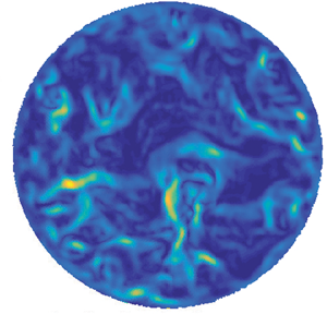
Figure 3. (a) Shear field,  $[\overline {A}]$, of an instantaneous snapshot of the cross-section of the pipe, where the shear values are normalized by the azimuthally averaged shear value at each wall-normal location, $[\overline {A}]_{{y}}$. (b) Intense shear regions of $[\overline {A}]$ (shown by black) greater than the $1.5\times$ local mean shear values for the same instantaneous snapshot in (a). Background map represents the instantaneous streamwise velocity field normalized by the central velocity of the pipe, ${u}/{U}_{{cl}}$.

Figure 4. Sample instantaneous field of the streamwise velocity,  ${u}$, normalized by ${U}_{cl}$ (colour map) in the wall-normal ( ${y}$)–streamwise ( ${x}$) plane together with the detected shear regions, $[A]$ (shown by the grey contours), normalized by the mean shear value at ${y}/{R}=0.2$. The streamwise extent is reconstructed using the bulk velocity, ${U}_{b}$, together with Taylor's hypothesis. Arrow indicates the direction of the flow.
Figure 3(a) shows the shear content,  $[\overline {A}]$, of an instantaneous snapshot of the cross-section of the pipe. Here, the local shear values are normalized by the azimuthally averaged shear values (for each radial position) of the same snapshot. This results in intense shear regions as can be seen in this figure. After applying a threshold, based on the $1.5\times$ local mean (figure 3b), these intense shear regions can be distinguished from the surrounding. Based on the thresholding criterion, the thickness and the spanwise length of the structures vary somewhat, as expected. However, they remain relatively thin compared to their spanwise length. The structures identified by the applied threshold in figure 3(b) are observed to surround the core region of the pipe, which is less turbulent than the region near the wall. A similar observation was reported before by Kwon et al. (Reference Kwon, Philip, de Silva, Hutchins and Monty2014) and Yang, Hwang & Sung (Reference Yang, Hwang and Sung2016) for a turbulent channel flow, where they argued that a continuous interface marking a jump in the streamwise velocity demarcates the quiescent core region. Also, the layers in the turbulent pipe flow are observed to be bounding large-scale regions of nearly uniform streamwise velocities (figures 3 and 4), as previously reported observations by Meinhart & Adrian (Reference Meinhart and Adrian1995), Adrian et al. (Reference Adrian, Meinhart and Tomkins2000) and Eisma et al. (Reference Eisma, Westerweel, Ooms and Elsinga2015) in a TBL.
Furthermore, to investigate the large-scale motions around the shear layers and possible link between them,  $3$-D conditional analyses were conducted. Figures 5(a) and 5(b) show iso-surfaces of the streamwise and wall-normal velocity fluctuations and swirling strength for the averaged flow field conditioned on the wall-normal centres of the internal shear layers in the range ${y}/{R}=0.15\text {--}0.2$. Here, for each cross-section of a detected shear layer in the spanwise–wall-normal plane, the shear layer was further divided into sections at each spanwise location. Finally, for each section of the shear layer the wall-normal centre was determined. While ${y}_i$ corresponds to the wall-normal centre of each final cross-section, ${x}_i$ and $\theta _i$ indicate the streamwise and azimuthal positions of these cross-sections, respectively. Hence, the flow field was remapped with respect to ${y}_i$, ${x}_i$ and $\theta _i$ for each cross-section of a shear layer. Here, local conditional mean streamwise velocities were used to reconstruct the streamwise extent. As can be seen in these $3$-D figures, below ( ${y}-{y}_i=0$) there is a strong low-speed region extending in the streamwise direction, which is accompanied by two distinguished swirling motions having opposite signs in the spanwise direction. Also, this low-speed region can be seen to be associated with strong positive wall-normal velocity fluctuations, which would indicate a region dominated by ejection events. These findings are consistent with the conceptual picture of Adrian et al. (Reference Adrian, Meinhart and Tomkins2000) in the sense that uniform low-speed regions are separated from other flow regions by strong vorticity, either in the form of shear layers, hairpins or both, and support the connection between the shear layers and the hairpin structures.

Figure 5. Iso-surfaces of the streamwise and wall-normal velocity fluctuations (a), and swirling motions together with the low-speed flow (b), that are remapped with respect to the wall-normal centres of the detected shear layers. Here, only the shear layers in the range  ${y}/{R}=0.15\text {--}0.2$ are considered; ${y}_i$, ${x}_i$ and $\theta _i$ correspond to the wall-normal, streamwise and azimuthal positions of the shear layers (cross-sectionwise), respectively. Blue, red, yellow and green surfaces in (a) correspond to $\langle {u}^\prime /{U}_{cl}\rangle =-0.03$, $\langle {u}^\prime /{U}_{cl}\rangle =0.015$, $\langle {v}^\prime /{U}_{cl}\rangle =-0.003$ and $\langle {v}^\prime /{U}_{cl}\rangle =0.006$, respectively. The streamwise extent is reconstructed using the local conditional mean streamwise velocities. Iso-surfaces in cyan and purple in (b) represent a swirling strength of $\langle \lambda {R}/{U}_{cl}\rangle =0.05$ and $\langle \lambda {R}/{U}_{cl} \rangle = -0.05$, respectively.
In addition to figure 5, in figure 6, a  $2$-D cross-section of some averaged flow fields at ( ${x}-{x}_i=0$) is provided in the spanwise–wall-normal plane for all components of the velocity fluctuations as well as swirling strength and Reynolds shear stress. All of the above findings in figure 5 can be more clearly seen in these $2$-D cross-sections. Furthermore, from the spanwise component of the averaged velocity fluctuations (figure 6c) as well as the averaged vector field shown by arrows and swirling motions (figures 6d and 6f), it can be seen that the shear layers are strongly stretched in the spanwise direction. This is the reason why the layers are thin in the wall-normal direction.

Figure 6. Conditionally averaged fields around the shear layers for (a) streamwise velocity fluctuation,  $\langle {u}^\prime /{U}_{cl}\rangle$, (b) wall-normal velocity fluctuation, $\langle {v}^\prime /{U}_{cl}\rangle$, (c) spanwise velocity fluctuation, $\langle {w}^\prime /{U}_{cl}\rangle$, (d) swirling strength, $\langle \lambda {R}/{U}_{cl}\rangle$ and (e) Reynolds shear stress, $\langle -{u}^\prime {v}^\prime /{U}^2_{cl}\rangle$. Panel (f) shows a close view for all components of the velocity fluctuations and swirling strength. Here, contour lines in blue, red, yellow, green, black, orange, purple and cyan correspond to $\langle {u}^\prime /{U}_{cl}\rangle =-0.03$, $\langle u^\prime /{U}_{cl}\rangle =0.015$, $\langle {v}^\prime /{U}_{cl}\rangle =-0.03$, $\langle {v}^\prime /{U}_{cl}\rangle =0.06$, $\langle {w}^\prime /{U}_{cl}\rangle =-0.06$, $\langle {u}^\prime /{U}_{cl}\rangle =0.06$, $\langle \lambda {R}/{U}_{cl}\rangle =-0.05$ and $\langle \lambda {R}/{U}_{cl}\rangle =0.05$, respectively. Arrows indicate the average vector field for $\langle {u}^\prime \rangle$ and $\langle {w}^\prime \rangle$. Results correspond to the plane ( ${x}-{x}_i=0$).
Note that we repeated the same conditional analysis for the shear layers at other wall-normal locations. The results are qualitatively similar for the velocity fluctuations and swirling motions. However, a decrease in the strength of these properties with the wall distance was observed.
3.3. Shear layers in the spanwise–wall-normal plane
Previously mentioned studies have examined the shear structures or the continuous edges of the UMZs in the streamwise–wall-normal plane only, either in a TBL or turbulent channel flow. In this section, we extend the analysis to the cross-sectional plane, and consider the properties of the shear layers in the spanwise direction, which latter has not been considered before.
We begin the analysis by conditionally averaging some flow properties across the shear layers in the spanwise direction. The shear layers were first divided into spanwise–wall-normal cross-sections at each streamwise location similar to § 3.2. Then, for each cross-section, the shear layers were further divided into sections at each wall-normal position, having a certain wall thickness determined by the vector spacing but varying spanwise length. Afterwards, with respect to its wall position, each section was grouped from the near wall,  ${y}=0.1{R}$, to the core, ${y}=1{R}$, of the pipe in bins with an equal increment of $0.1{R}$. Finally, relative to the spanwise centre of each section, conditional analyses were performed to find out if there is any change in the flow properties across the detected shear layers along the spanwise direction. The resulting average profiles for the streamwise velocity, $\langle {u}\rangle$, and the dissipation rate, $\langle \varepsilon \rangle$ are shown in figure 7. Here, the profiles in (a,b) are normalized by the local conditional-mean values of $\langle {u}\rangle _{y}$ and $\langle \varepsilon \rangle _{y}$, respectively, obtained at locations away from the effect of the layers. From figure 7, it can be seen that these structures are associated with low streamwise velocity and high dissipation. As can be seen in (a), this effect is stronger near the wall and weaker towards the core of the pipe; whereas in (b) similar peaks (in terms of the magnitude) in the dissipation rates result at each wall-normal location. Moreover, the peaks in the streamwise velocity and dissipation rate profiles are wider in terms of the azimuthal angle near the pipe centre. Note that the resolved dissipation rate was estimated by $\varepsilon _{resolved}= \frac {1}{2}\nu \overline {(u^\prime _{i,j}+u^\prime _{j,i})^2}$ (Tennekes & Lumley Reference Tennekes and Lumley1972), where $u^\prime _{i,j}$ denote the gradients of the velocity fluctuations. The gradients in the streamwise direction were determined using Taylor's hypothesis together with the local mean velocity. Since the dissipation rate was not fully resolved ( $45\,\%$ near the core of the pipe), the unresolved dissipation was estimated by the large eddy (Smagorinsky) model (Sheng, Meng & Fox Reference Sheng, Meng and Fox2000; Sharp & Adrian Reference Sharp and Adrian2001; Tokgoz et al. Reference Tokgoz, Elsinga, Delfos and Westerweel2012). The data in figure 7 represent the total dissipation, i.e. the sum of the resolved and unresolved dissipation.

Figure 7. Conditionally sampled streamwise velocity,  ${u}$, (a) and dissipation, $\varepsilon$, (b) profiles in the spanwise direction, $\theta$. The spanwise centre of each cross-section of the detected shear region is represented by $\theta _i$, while ( $\theta -\theta _i$) represents the distance from the centre of the cross-section of the layers in the spanwise direction. Shear layers are grouped according to the location of their spanwise centre (for each cross-section) in the pipe, from $0.1{R}$ to $1{R}$ with a constant increment of $0.1{R}$.
To check the spanwise width of the shear layers, two-point correlations for the gradient of the streamwise velocity,  ${R}({u}_{y}{u}_{y})$ were computed; ${R}({u}_{y}{u}_{y})$ can also provide information about the wall-normal thickness of the shear layers in an average sense. Here, in addition to correlations conditioned on the wall-normal centres (see § 3.2) of the shear layers (3.1), general correlations (3.2) conditioned on wall-normal locations irrespective of whether a shear layer is detected or not were also determined for comparison. For the latter, the wall-normal locations, ${y}_{ref}$, correspond to the centre of each bin that the detected shear layers are grouped into. The subscripts $\textit {s}$ and ref in (3.1) and (3.2) correspond to the properties related to the detected shear layers and reference wall locations, respectively. The overbars, on the other hand, represent conditional averaging over $\theta$ and ${x}$.
The wall-normal thickness and the spanwise length of these two-point correlations were quantified based on the peak width at  ${R}({u}_{y}{u}_{y})=0.8$. This threshold is relatively high to ensure converged results at each wall-normal location and because R does not drop to zero at large distances but reaches a plateau due to the mean gradient (see figure 8). The wall-normal thickness of the correlation is determined at the spanwise centre of the correlation, i.e. $(\theta -\theta _i=0)$ (see figure 8a,b), while the spanwise length is determined at the wall-normal centre of the correlation coefficient $({y}-{y}_{i}=0)$ (see figure 8c,d). Here, $\theta _i$ and ${y}_{i}$ represent the azimuthal (in terms of angles) and wall-normal locations of the detected shear, respectively.
 \begin{gather} {R}({u}_y{u}_{y,s})=\frac{\overline{{u}_y({x,y}_{s}, {z})\,{u}_y({x,y}, {z}+{r}_z)}}{\sqrt{\overline{{u}^2_{y}({y}_{s})}}\, \sqrt{\overline{{u}^2_{y}({y})}}}, \end{gather}
 \begin{gather} {R}({u}_y{u}_{y,ref})=\frac{\overline{{u}_y({x,y}_{ref}, {z})\,{u}_y({x,y}, {z}+ {r}_z)}}{\sqrt{\overline{{u}^2_{y}({y}_{ref})}}\,\sqrt{\overline{{u}^2_{y}({y})}}} . \end{gather}
Figure 8. Sketch illustrating how the wall-normal thickness,  ${l}_{y}$, (a,b) and the spanwise length, ${l}_{z}$, (c,d) of the correlation coefficients are determined using the peak width at ${R}({u}_{y}{u}_{y})=0.8$.
Dashed lines on the correlation contours indicate the wall-normal (a) and the spanwise (c) centres of the shear layers where
${R}({u}_{y}{u}_{y})=0.8$.
Dashed lines on the correlation contours indicate the wall-normal (a) and the spanwise (c) centres of the shear layers where  $ R({u_y}{u_y}) $ in (b,d), respectively, was determined; ${r}$ indicates the distance of the centre of the averaged shear layers from the core of the pipe.
The resulting width and the spanwise length of the two-point correlations are presented in figures 9(a) and 9(b), respectively, for several wall-normal locations and for all Reynolds numbers. Full lines with open symbols correspond to the data conditioned on the wall-normal centre of the shear layers, while the dashed lines with filled symbols represent the results for general conditioning on wall-normal location. When the general conditioning is compared to those for conditioning on the shear layers, a significant increase in the wall-normal thickness ( ${\sim }40\,\%$) and the spanwise length ( ${\sim }50\,\%$) of the correlation coefficient is observed for the case of the shear layers (see also figure 12b,c). The shear layers have, therefore, a significantly larger coherence length than can be expected from general unconditional correlations. On the other hand, although the presence of the shear layers significantly affects the size of the correlation peaks, the trends with wall-normal distance are quite similar. For both conditions, the wall-normal widths of the correlations are proportional to the Reynolds number until the wall-normal position of ${y}/{R}\approx 0.6$. Beyond that position, the behaviour reverses. Similar behaviour is observed for the spanwise length of the correlation coefficients below the same wall-normal position, i.e. ${y}/{R}\approx 0.6$, such that the spanwise length is proportional to the Reynolds number. Beyond this wall-normal location, the spanwise length appears to be independent of the Reynolds number.

Figure 9. Wall-normal thickness,  ${l}_{y}$, (a) and the spanwise length, ${l}_{z}$, (b) as determined from the peak (see figure 8). Full lines with open symbols are for the correlation conditioned on the wall-normal centre of the shear layers, and dashed lines with filled symbols are for the general correlation at reference wall locations. Yellow (diamond), blue (circle), red (triangle) and green (square) correspond to the flow conditions at $\mathit {Re}_{\tau }=340$, $752$, $999$ and $1259$, respectively.
As a final note in this section, the spanwise shape of the shear layers was also investigated through the two-point correlations for  $[A]$. However, similar results were obtained as the correlations for the streamwise velocity gradients.
3.4. Shear layers in the streamwise–wall-normal plane
In this section, the shear layers are examined in the streamwise–wall-normal plane. First, the detected shear layers were grouped according to the wall-normal distance of their centre as in § 3.2, and then conditional sampling was performed to analyse these structures in wall-normal–streamwise planes. The conditionally averaged profiles for the streamwise velocity  $\langle {u}\rangle$, wall-normal velocity $\langle {v}\rangle$, turbulent shear stress $\langle -{u}^\prime {v}^\prime \rangle$ and dissipation rate $\langle \varepsilon \rangle$, at ( ${x}-{x}_{i}$) are shown in figure 10. From the streamwise velocity (a) and dissipation rate (b) profiles, a significant increase is observed within the averaged layers at each wall-normal location, the magnitude of which is decreasing towards the core of the pipe. For the turbulent shear stress profiles (d), on the other hand, a decrease in the magnitude across the sampled layers is observed. Although these averaged streamwise velocity and turbulent shear stress profiles in the turbulent pipe flow are consistent with those for TBLs (e.g. Eisma et al. Reference Eisma, Westerweel, Ooms and Elsinga2015; Laskari et al. Reference Laskari, de Kat, Hearst and Ganapathisubramani2018), there is a significant difference in the trend of the wall-normal velocity profiles. The magnitude of the conditional wall-normal velocities across the shear layers in these TBL studies keep increasing with wall distance, whereas similar magnitudes were observed in the pipe flow at each wall-normal position (figure 10c). This could be explained by the effect of the flow confinement in the pipe flow, which is different from the TBL.

Figure 10. Conditionally sampled streamwise velocity  $\langle {u}\rangle$ (a), dissipation $\langle \varepsilon \rangle$ (b), wall-normal velocity $\langle v\rangle$ (c) and turbulent shear stress $\langle -{u}^\prime {v}^\prime \rangle$ (d) profiles. The centre of the shear region is represented by ${y}_{i}$, while ( ${y}-{y}_{i}$) represents the distance from the centre of the layers in the wall-normal direction. Shear layers are grouped according to the location of their centres in the pipe, from $0.1{R}$ to $1{R}$ with a constant increment of $0.1{R}$. The arrow shows the direction of the wall (from $1{R}$ to $0.1{R}$).
The jumps in the streamwise velocities are further quantified for each  $\mathit {Re}_\tau$, and for each wall-normal bin using a method similar to the one of Chauhan et al. (Reference Chauhan, Philip, de Silva, Hutchins and Marusic2014) (figure 11). The single set and three set results for $\mathit {Re}_\tau =752$ are nearly identical, which implies that the results appear to be converged. Furthermore, it can be seen that the jumps in the conditional streamwise velocity profiles at each wall-normal location are very similar for different Reynolds numbers, except for $\mathit {Re}_\tau =340$ near the wall. This is consistent with the findings of de Silva et al. (Reference de Silva, Philip, Hutchins and Marusic2017), who showed that the velocity jumps across the UMZ edges within a TBL are independent of the Reynolds number ( $\mathit {Re}_\tau =10^3\text {--}10^4$ in their study), when scaled by $u_\tau$. The present study supports this argument also in a turbulent pipe flow at much lower Reynolds numbers. Moreover, these jumps are observed to be strong near the wall and decrease towards the core of the pipe. This is again consistent with the observations in the above mentioned TBL study. Stronger jumps near the wall for $\mathit {Re}_\tau =340$ can be explained by the low Reynolds number effect, as also observed in a very recent DNS study ( $\mathit {Re}_\tau =500$) of Chen et al. (Reference Chen, Yongmann and Wan2020) in a turbulent pipe flow. Based on the conditional streamwise velocity profiles (figure 10a), the thickness of the layers is also determined (figure 11). It can be seen that the thickness of the layers is in the range $0.05\text {--}0.09{R}$. Note that the normalization does not imply that the thickness scales with R. The present limited Reynolds number range does not allow for a detailed scaling analysis.

Figure 11. (a) Schematic showing how the velocity jumps and thicknesses of the layers are determined using a method similar to the one of Chauhan et al. (Reference Chauhan, Philip, de Silva, Hutchins and Marusic2014). (b) Jumps in the streamwise velocity profiles at several wall locations,  ${\rm \Delta} {U}$, which are normalized by ${u}_\tau$. (c) Thickness of the shear layers at the same wall-normal locations. Yellow (diamond), blue (circle), red (triangle) and green (square) colours correspond to the flow conditions at i.e. $\mathit {Re}_\tau =340$, $752$, $999$ and $1259$, respectively. Additionally, filled circles correspond to data with three independent sets for $\mathit {Re}_\tau =752$.
Similar to the previous section, two-point correlations for the gradients of the streamwise velocity were performed in wall-normal–streamwise planes to determine the effect of the shear structures on the streamwise length of the correlation coefficient peaks. Similar to the thickness and the spanwise length of the correlation peaks, a significant increase in the streamwise length of the correlation coefficients is visible when conditioning on the shear layers. When the streamwise length scale determined from the width of the correlation peaks based on  ${R}({u}_{y}{u}_{y})=0.8$ is compared for all $\mathit {Re}_\tau$ (figure 12a), it can be seen that the increase is around $40\,\%$ (figure 12d).

Figure 12. (a) Streamwise length,  ${l}_{x}$, of the peak of the correlation coefficients. Full lines with open symbols are for the correlation conditioned on the wall-normal centre of the shear layers, and dashed lines with filled symbols are for the general correlation at reference wall locations. Panels (b–d) show percentage increase in the width of the correlation peaks with the presence of the shear layers in the wall-normal, spanwise and streamwise directions, respectively.
4. Edges of UMZs using different orientation of planes
In § 3, the properties of the internal shear layers identified using a  $3$-D detection scheme were discussed in detail. The results revealed that these highly dissipative structures are elongated in both the streamwise and spanwise directions. Furthermore, the internal shear layers are bounded by large-scale regions of nearly uniform velocities. This strongly suggest that the shear layers are the edges of the so-called uniform momentum zones. Therefore, in this section, we detect and analyse the edges of the UMZs for later comparison with the internal shear layers § 5.
The UMZs are basically large-scale regions identified by employing the histogram approach of Adrian et al. (Reference Adrian, Meinhart and Tomkins2000) and de Silva et al. (Reference de Silva, Hutchins and Marusic2016). With this current work, we aim to provide a comparison between these two different detection methods for the shear layers in a statistically steady turbulent pipe flow. In previous studies (e.g. Kwon et al. Reference Kwon, Philip, de Silva, Hutchins and Monty2014; de Silva et al. Reference de Silva, Hutchins and Marusic2016; Laskari et al. Reference Laskari, de Kat, Hearst and Ganapathisubramani2018), the edges of the UMZs were analysed in wall-normal–streamwise planes (and for  $2$-D data only). Here, the analysis is extended to other orientations of the planes, i.e. wall-normal–streamwise versus wall-normal–spanwise planes, when using the histogram method. Furthermore, with all the UMZ edges determined from the wall-normal–streamwise planes at different azimuthal positions across the pipe, the cross-stream connectivity of the UMZ edges can also be explored, which also allows us to assess the consistency of the method.
4.1. Edges of the UMZs in the streamwise–wall-normal plane
In this section, we use the streamwise–wall-normal plane to plot the histogram of the streamwise velocities, and accordingly detect the continuous edges of the UMZs. The wall-normal plane extends from  ${y}=0.05{R}$ to the core of the pipe ( ${y}={R}$). The streamwise extent of the plane, on the other hand, is limited to ${\sim }2.2{R}$ (explained below) for each flow condition considered in this section. Since the data were acquired in the cross-section of the pipe with time-resolved stereoscopic PIV, the streamwise length was reconstructed using Taylor's hypothesis with the bulk velocity as the convection velocity. Following de Silva et al. (Reference de Silva, Hutchins and Marusic2016), the location of an UMZ edge was approximated by the streamwise velocity contour corresponding to the mid-point between the local peaks in the histogram of the streamwise velocities. Figure 13(a) shows a sample field of the streamwise velocity together with the UMZ edges (black lines), and panel (b) shows the corresponding histogram of the streamwise velocities over this plane. The local peaks on the histogram correspond to the so-called modal velocities, and the locations of the UMZ edges in (a) were the mid-point between these modal velocities. The regions demarcated by these edges, i.e. R1, R2 and R3, are called UMZs, since within each region the magnitude of streamwise velocity is nearly constant. Note that the histogram of the streamwise velocities was not much affected by peak locking. Therefore, the raw data without any smoothing were used throughout § 4.

Figure 13. (a) Sample instantaneous field of the streamwise velocity, u, normalized by the central velocity of the pipe,  ${U}_{cl}$, together with the detected UMZs and their edges on a wall-normal–streamwise plane. (b) The corresponding histogram of the streamwise velocities over the plane shown in (a). R1, R2 and R3 show three different regions with similar velocities (UMZs), while the black continuous lines in (a) correspond to the mid-points between the peaks in the p.d.f. as indicated by the dashed lines in (b).
In this section, all the streamwise velocities over each plane were distributed over 50 histogram bins, which corresponds to a bin size of  ${\sim }0.12{U}_{cl}$ for all the cases considered. In addition, to correctly identify the modal velocities and accordingly the edges of the UMZs, the greater of the peaks that were separated by only a single histogram bin was chosen as the peak, and the smaller one was ignored. Furthermore, peaks whose count was less than $0.5\,\%$ of the total number of the data points in the considered plane were also ignored to avoid noisy peaks affecting the identification of UMZs close to the wall. It should also be noted here that the modal velocities are highly dependent on the number of histogram bins. If the number of bins increases, then more modal velocities and UMZ edges are identified. However, the locations of the detected UMZ edges become very close to each other, such that the distance between them becomes less than the thickness of the shear layers discussed previously.
Another important parameter affecting the number and the location of the UMZ edges is the streamwise extent of the considered plane. If the streamwise length of the plane is very long then no separation between the regions of similar velocities occurs, since the histogram would average to its mean, which is resulting in a single peak. On the other hand, if the streamwise length is very short then the total number of data points in the plane is not enough to accurately define the UMZs and their edges. In this study, a streamwise length ( ${\sim }2.2{R}$) was chosen after conducting several analyses with different streamwise lengths, ranging between $1.2{R}$ and $2.5{R}$. The results revealed that, although the number density of the UMZ edges varied with the size of the streamwise distance, the overall statistics were observed to be almost identical over the ranges considered. Therefore, to have enough data points for each flow condition, a streamwise length ${\sim }2.2{R}$ was employed. This length corresponds to ${\rm \Delta} {x}^+\approx 752$, $1682$, $2208$ and $2798$ for $\mathit {Re}_\tau =340$, $752$, $999$ and $1259$, respectively. Furthermore, there are a total of 52, 384, 180 and 232 independent streamwise–wall-normal planes for these Reynolds numbers, $\mathit {Re}_\tau =340$, 752, 999 and $1259$, respectively. These numbers have been established assuming four azimuthal planes are independent of each other and considering that the streamwise length of the shear layers ( ${\sim }{R}$, see § 3) is shorter than the ${\sim }2.2{R}$ streamwise length of each plane, such that non-overlapping planes in the streamwise direction are independent.
In this section, the azimuthal continuity of the detected modal velocities was also used as an additional criterion on the peaks of the histogram plots. Compared to the base case (case A), where no azimuthal condition is applied, for case B only the peaks that also appeared at least on one of the neighbouring wall-normal–streamwise planes are considered. The azimuthal spacing between two neighbouring planes is  $0.01{R}$ (arc length) at the wall, which is much smaller than the thickness of the internal shear layers. For case C, on the other hand, the peaks on the histogram of the base plane were required to repeat on two other consecutive planes located azimuthally either before or after the current azimuthal position. Note that, throughout this section, unless otherwise stated, the results using the first azimuthal criterion (case B) are presented.
Figure 14 shows the resulting p.d.f. of the number of the UMZs in a plane for each Reynolds number and also for the different azimuthal conditions (cases A, B and C, mentioned above). It can be seen that the distributions are not very sensitive to the azimuthal condition. Similar behaviour with respect to the azimuthal condition is also observed in the p.d.f.s of the velocities corresponding to the location of the identified UMZ edges, and of the modal velocities. For brevity, only the results for case B are shown in figure 15. From these plots it can also be seen that a significant number of the velocities corresponding to the location of the UMZ edges appear around  $95\,\%$ of the central velocity of the pipe, ${U}_{cl}$, while the modal velocity p.d.f.s peak at ${U}_{cl}$. Similar behaviour was also reported previously by Kwon et al. (Reference Kwon, Philip, de Silva, Hutchins and Monty2014) for a turbulent channel flow using a similar histogram approach.

Figure 14. The p.d.f. of the number of the detected UMZs over the wall-normal–streamwise planes with case A (a), case B (b) and case C (c). Yellow (diamond), blue (circle), red (triangle) and green (square) correspond to the flow conditions at  $\mathit {Re}_\tau =340$, $752$, $999$ and $1259$, respectively.

Figure 15. The p.d.f. of the velocities corresponding to the location of the UMZ edges,  ${U}_{i}/{U}_{cl}$, (a) and the p.d.f. of the modal velocities, ${U}_{m}/{U}_{cl}$, (b). Yellow, blue, red and green correspond to the flow conditions $\mathit {Re}_\tau =340$, $752$, $999$ and $1259$, respectively. Results for case B are presented here.
Finally, in this section, the UMZ edges detected over the wall-normal–streamwise planes at each of the azimuthal planes were projected onto the cross-section of the pipe for each flow condition (figure 16). It can be seen that for the lowest Reynolds number (i.e.  $\mathit {Re}_\tau =340$), the UMZ edges are coherent in the spanwise direction and separating the regions of similar velocities in the cross-section of the pipe, in the same way as in the wall-normal–streamwise planes where they were originally identified. The same applies to the results obtained at other Reynolds numbers. However, the continuity of the UMZ edges in the spanwise direction is not as clear as those for $\mathit {Re}_\tau =340$. This is partly due to the noisy peaks in the histogram at higher Reynolds number, which could be a result of the decreased spatial resolution in the streamwise direction, hence, a smaller number of velocity points in a given area. Moreover, the undulation of the velocity contours, hence UMZ edges, appear at increasingly smaller scale as the Reynolds number increases, which affects the smoothness of the edge in the spanwise direction.

Figure 16. The projection of the edges of the UMZs, which were detected using the streamwise–wall-normal plane, onto the wall-normal–azimuthal plane (black regions) for the flow conditions  $\mathit {Re}_\tau =340$ (a), $\mathit {Re}_\tau =752$ (b), $\mathit {Re}_\tau =999$ (c) and $\mathit {Re}_\tau =1259$ (d). Background colour shows the instantaneous streamwise velocity field normalized by the central velocity ${U}_{cl}$.
4.2. Edges of the UMZs in the spanwise–wall-normal plane
In this section, the UMZs and their edges were detected over the cross-section of the pipe. In this case, the UMZs and their edges were detected using the histogram of the streamwise velocities in the spanwise–wall-normal plane where the bin size was  ${\sim }0.12{U}_{cl}$. As before, the locations of the UMZ edges on that plane were identified by considering the mid-point between the local peaks in the histogram (figure 17). For the histogram peaks that were separated by a single bin, the greater one was selected as before (§ 4.1).

Figure 17. (a) Sample instantaneous field of the streamwise velocity, u, normalized by the central velocity of the pipe,  ${U}_{cl}$, together with the detected UMZs and their edges on a wall-normal–spanwise plane. (b) The corresponding histogram of the streamwise velocities over the plane shown in (a). R1, R2, R3, R4 and R5 show five different regions of similar velocities (UMZs), while the black continuous lines in (a) correspond to the location of the UMZ edges determined by the dashed lines in (b).
As can be seen in figure 18(a), similar distribution for the total number of the UMZs in the cross-section is observed for all the considered flow conditions. These distributions are also consistent with those, except for  $\mathit {Re}_\tau =340$, presented in figure 14 based on the detection in the streamwise–wall-normal plane. Also, the p.d.f.s of the velocities corresponding to the UMZ edges are quite similar to those obtained in the streamwise–wall-normal plane (compare figures 18b and 15). Again, the velocities corresponding to the UMZ edges are mostly appearing around $95\,\%{U}_{cl}$, bounding the relatively less turbulent core region of the pipe.

Figure 18. (a) The p.d.f. of the number of UMZs detected using the spanwise–wall-normal planes. (b) The p.d.f. of the instantaneous velocities corresponding to the location of the detected UMZ edges. Yellow (diamond), blue (circle), red (triangle) and green (square) symbols correspond to the flow conditions  $\mathit {Re}_\tau =340$, $752$, $999$ and $1259$, respectively.
Note that the UMZs are continuous by the definition of their edges as iso-contours of streamwise velocity. Each UMZ exists all the way around the circumference, because the associated velocity contours do. The latter is not surprising. The former (UMZs spanning the circumference) may be considered dubious, which would imply that the commonly used UMZ detection method is problematic. Nevertheless, the p.d.f. method is adopted for consistency with the existing literature. Furthermore, the method is suitable for showing that shear layers are found at the edges of large, nearly uniform, momentum regions (see § 5).
5. Comparison of the UMZ edges and the shear layers
In this part, the edges of the UMZs and the identified shear layers are compared both visually and quantitatively. Figures 19 and 20 provide a visual comparison of the UMZ edges detected using a different orientation of the planes and the shear layers. These figures present the results for  $\mathit {Re}_\tau =340$ and for $\mathit {Re}_\tau =752$, respectively, to allow for comparison between two different Reynolds numbers. From the contour plots in figures 19(b) and 20(b), it can be seen that the shear layers appear on the continuous edges of the UMZs which were detected using the cross-section p.d.f. (wall-normal–spanwise plane). Although the shear layers are not fully connected in the azimuthal direction as are the UMZ edges, they have a significant azimuthal length. Note that the UMZs are by their definition as velocity contours. When the UMZ edges that were detected from wall-normal–streamwise planes are compared with the shear layers (see figures 19c and 20c), it can also be seen that they correspond mostly to the regions of intense shear. Furthermore, the azimuthal extent of the densely populated regions of the UMZ edges (magenta) is seen to be comparable to the azimuthal length of the shear layers.

Figure 19. Comparison of the shear layers detected using the  $3$-D method (black regions), edges of the UMZs defined using the wall-normal–spanwise planes (black contour lines) and the projection of the UMZ edges identified over the wall-normal–streamwise planes (magenta regions). Panels (a–d) show different combinations of the UMZ edges and the shear layers for better comparison. Results correspond to the flow condition at $\mathit {Re}_\tau =340$, and background colour map shows the instantaneous streamwise velocity normalized by ${U}_{cl}$.

Figure 20. Comparison of the shear layers detected using the  $3$-D method (black regions), edges of the UMZs defined using the wall-normal–spanwise planes (black contour lines) and the projection of the UMZ edges identified over the wall-normal–streamwise planes (magenta regions). Panels (a–d) show different combinations of the UMZ edges and the shear layers for better comparison. Results correspond to the flow condition at $\mathit {Re}_\tau =752$, and background colour map shows the instantaneous streamwise velocity normalized by ${U}_{cl}$.
Based on the visualizations it appears that the shear layers coincide with the edges of the UMZs, similar to the observations in previous studies (Meinhart & Adrian Reference Meinhart and Adrian1995; Adrian et al. Reference Adrian, Meinhart and Tomkins2000; Eisma et al. Reference Eisma, Westerweel, Ooms and Elsinga2015). This correspondence is quantified by considering the distance from the core of a shear region to the nearest edge of the UMZs (defined over the wall-normal–streamwise plane). It is found that this distance is less than  $0.035R$ (figure 21a), which is smaller than the thickness of the shear layers ( ${\sim }0.07R$, see figure 11c). When the locations of the core of the shear layers are compared with those of the UMZ edges defined over the cross-section of the pipe, it can be seen that all the shear layers reside in close proximity to these UMZ edges; see figure 21(b). For the distance between the UMZ edges determined over the two different orientations of planes, it can be seen in figure 21(c) that the distance is greater than in the previous two cases. These results show that the shear layers detected by the $3$-D method have a very good overlap with the UMZ edges detected by the histogram method. However, the reverse is not the case. This is obvious for the UMZ edges determined from the cross-section of the pipe, since the shear layers are not continuous in the azimuthal direction. For the UMZ edges determined from the wall-normal–streamwise planes, these UMZ edges do not always correspond to a detected shear layer. It should also be noted that the results are quite similar over the range of the Reynolds numbers considered.

Figure 21. The p.d.f. of the distance of the core of the shear layers from the UMZ edges of the UMZs defined using the wall-normal–streamwise planes (a) and using the wall-normal–spanwise planes (b). (c) The p.d.f. of the distance of the UMZ edges determined in wall-normal–streamwise planes to the UMZ edges detected using the wall-normal–spanwise planes. (d) The p.d.f. of the number of UMZs which were determined based on the occurrence of shear layers at each spanwise and streamwise direction. Yellow (diamond), blue (circle), red (triangle) and green (square) correspond to the flow conditions  $\mathit {Re}=340$, $752$, $999$ and $1259$, respectively.
Finally, when the p.d.f. of the number of the UMZs that were determined based on the occurrence of the shear layers (figure 21d) is compared with those in figures 14 and 18(a), a very similar distribution was found. Here, the UMZs were defined according to the wall-normal centre of the detected shear layers as in § 3.2. These results also suggest that the distribution for the number of the UMZs does not change significantly with Reynolds number in a turbulent pipe flow; at least within the range of the Reynolds numbers considered in this study, no significant variation was found. However, it should be noted that the range of Reynolds number in the present study is small. The number distribution of UMZs with Reynolds number was investigated before by de Silva et al. (Reference de Silva, Hutchins and Marusic2016) in a TBL, and they found a log linear increase of the number of the UMZs with Reynolds number. In their study, a larger range of Reynolds number,  $\mathit {Re}_\tau =10^3\text {--}10^4$, was investigated. As a final note in this section, the number distribution of the UMZs found in this study is very similar to the one reported very recently by Chen et al. (Reference Chen, Yongmann and Wan2020) in a turbulent pipe flow at $\mathit {Re}_\tau =500$, where the UMZs were determined using 3-D volumetric data.
6. Conclusions
In this paper, a comprehensive analysis is presented of the properties of the internal shear layers and the edges of the UMZs in a turbulent pipe flow. The experimental datasets used were acquired with time-resolved stereoscopic PIV in the cross-section of the pipe for four different Reynolds numbers,  $\mathit {Re}_\tau =340$, $752$, $999$ and $1259$. For each flow condition, the shear layers were detected using the method of Horiuti & Takagi (Reference Horiuti and Takagi2005), which enabled us to investigate the $3$-D features of these structures. The UMZs and their edges, on the other hand, were determined using the histogram method following de Silva et al. (Reference de Silva, Hutchins and Marusic2016).
Visual examples of the shear layers together with the corresponding instantaneous velocity fields showed clearly observable regions of similar streamwise velocities bounded by the detected shear layers both in the spanwise–wall-normal and stream wise–wall-normal planes. In particular, the core region of the pipe, which had relatively low turbulence, was seen to be bounded by the layers. Also, the shear layers were observed to be elongated in the streamwise directions ( ${\sim }{R}$), and they appear arc-like in the cross-sectional planes.
The conditional mean flow around the shear layers revealed a low-speed region beneath the average shear layers. This low momentum flow was associated with positive wall-normal velocity fluctuations, and surrounded by two oppositely rotating swirling motions on either side in the azimuthal direction. The shear layers were observed to be stretched in the azimuthal direction by two oppositely signed secondary motions, keeping the layers thin in the wall-normal direction. These findings are consistent with the conceptual picture of Adrian et al. (Reference Adrian, Meinhart and Tomkins2000) in the sense that uniform low-speed regions are separated from other flow regions by strong vorticity, either in the form of shear layers, hairpins or both, and support the connection between the shear layers and the hairpin structures.
Moreover, conditional averaging across the detected shear layers revealed significant jumps in the flow properties (e.g. turbulent shear stress, streamwise and wall-normal velocities) occurring in the wall-normal direction. Furthermore, these shear layer regions are highly dissipative.
Further analysis on the shear layers was performed through two point spatial correlations to reveal if and how much they affect the surrounding flow in an average sense. The two-point correlations were conditioned on the wall-normal centre of the shear layers, where the shear layers were grouped into according to their wall-normal centre. For comparison, general correlations (i.e. not conditioned on shear layers) were also evaluated for a given wall-normal reference position. The resulting correlations revealed that the shear layers significantly affect the average size of the correlation peaks in all directions. Moreover, it was seen that the streamwise length of the structures are of the same order as the large-scale motions, which support the argument that the shear layers are bounding the large-scale motions, i.e. UMZs.
In the second part of the work, the continuous edges of UMZs were detected using the histogram method. The histogram approach has been frequently employed in the literature. However, the analysis has been limited to the wall-normal–streamwise planes at a single spanwise position, over which the histogram is constructed using the streamwise velocity information. Therefore, the spanwise length of the UMZ edges could not be obtained. With the current work, on the other hand, the UMZ edges that were obtained over the wall-normal–streamwise planes at each azimuthal position were projected onto the cross-section of the pipe. With this approach, the spanwise extent of the UMZ edges could be visualized. The results showed that the UMZ edges appear to be coherent in the spanwise direction (when the densely populated regions of the UMZ edges are considered).
Furthermore, different than in previous studies, the wall-normal–spanwise plane was also used to investigate the UMZ edges in the cross-section of the pipe. The histogram analysis revealed UMZ edges that are similar to the findings based on the histograms from the wall-normal–streamwise planes. In the last part of this work, the UMZ edges defined using the histogram approach with two different orientations of the planes were compared with each other, as well as the shear layers that were detected using the  $3$-D method. Both visual results and the quantitative analysis showed that the detected shear layers coincide with the UMZ edges, such that the distance of the core of the shear layers from the UMZ edges defined in the cross-section of the pipe was found to be much smaller than the thickness of the shear layers. However, since the spanwise and streamwise lengths of the intense shear regions do not appear as long as the UMZ edges, which is partly explained by the different nature of their detection methods, the reverse does not hold: the detected UMZ edges through the histogram method do not always appear to overlap with the shear layers as defined by the $3$-D method.
Acknowledgements
This work is part of the research programme of the Foundation for Fundamental Research on Matter (FOM), which is part of the Netherlands Organisation for Scientific Research (NWO).
Declaration of interests
The authors report no conflict of interest.


 Open access