


Introduction
Body size is a key morphological variable that plays a significant role in biology and ecology (Peters Reference Peters1983; Schmidt-Nielsen Reference Schmidt-Nielsen1984; Barbault Reference Barbault1988; Damuth Reference Damuth1991; Cotgreave Reference Cotgreave1993; Blackburn and Gaston Reference Blackburn and Gaston1994; Brown Reference Brown1995; Calder Reference Calder1996; Jablonski et al. Reference Jablonski, Jablonski, Erwin and Lipps1996; Payne et al. Reference Payne, Boyer, Brown, Finnegan, Kowalewski, Krause, Lyons, McClain, McShea and Novack-Gottshall2009; Petchey and Belgrano Reference Petchey and Belgrano2010). Numerous studies have documented size diminution of individuals in the recovery phases following mass extinction events (Schmidt et al. Reference Schmidt, Thierstein and Bollmann2004; Payne Reference Payne2005; Aberhan et al. Reference Aberhan, Weidemeyer, Kiessling, Scasso and Medina2007; Twitchett Reference Twitchett2007; Harries and Knorr Reference Harries and Knorr2009). This phenomenon, widely known as the Lilliput effect, was first recognized in several graptolite taxa after relatively small-scale biological crises during the late Silurian (Urbanek Reference Urbanek1993). Similar size reductions are seen in several other faunal groups in postextinction strata, for example, Ordovician–Silurian crinoids (Borths and Ausich Reference Borths and Ausich2011), terminal Ordovician brachiopods (Huang et al. Reference Huang, Harper, Zhan and Rong2010), early Silurian corals (Kaljo Reference Kaljo1996), Late Devonian conodonts (Renaud and Girard Reference Renaud and Girard1999) and echinoids (Jeffery and Emlet Reference Jeffery and Emlet2010), and late Guadalupian fusulinoidean fusulinid foraminifers (Payne et al. Reference Payne, Groves, Jost, Nguyen, Moffitt, Hill and Skotheim2012; Groves and Wang Reference Groves and Wang2013). However, the mechanisms of size change remain controversial. Four biological circumstances were proposed to account for the potential Lilliput effect after the Permian–Triassic mass extinction (PTME): (1) size-based extinction, (2) size-based origination, (3) changing relative abundances, and (4) size change within lineages (Payne Reference Payne2005; see also Twitchett Reference Twitchett2007; Song et al. Reference Song, Tong and Chen2011). In addition, the relative proportion of within- and among-lineage processes in changing body size was compared quantitatively by Rego et al. (Reference Rego, Wang, Altiner and Payne2012), who concluded that size reduction within lineages rather than size-biased extinction drove the Lilliput effect following the PTME.
The PTME was the most severe biotic crisis of the Phanerozoic, during which the Paleozoic Fauna was replaced by the Modern Fauna (Sepkoski et al. Reference Sepkoski, Bambach, Raup and Valentine1981; Bottjer et al. Reference Bottjer, Clapham, Fraiser and Powers2008; Erwin Reference Erwin2015). More than 90% of all marine species and >70% of terrestrial species were eliminated during the crisis (Raup Reference Raup1979; Erwin Reference Erwin1993; Jin et al. Reference Jin, Wang, Wang, Shang, Cao and Erwin2000; Benton Reference Benton2003; Song et al. Reference Song, Wignall, Tong and Yin2013), leading to the “reef gap” (Flügel and Kiessling Reference Flügel and Kiessling2002; Kiessling et al. Reference Kiessling, Kustatscher, Preto and Wignall2010), a flat latitudinal biodiversity gradient (Song et al. Reference Song, Huang, Jia, Dai, Wignall and Dunhill2020), and a reversed functional pyramid in the Early Triassic oceans (Song et al. Reference Song, Wignall and Dunhill2018). Many kinds of (often synergistic) environmental stresses have been implicated in the crisis, including global warming (Kidder and Worsley Reference Kidder and Worsley2004; Joachimski et al. Reference Joachimski, Lai, Shen, Jiang, Luo, Chen, Chen and Sun2012; Sun et al. Reference Sun, Joachimski, Wignall, Yan, Chen, Jiang, Wang and Lai2012), hypercapnia (Knoll et al. Reference Knoll, Bambach, Canfield and Grotzinger1996, Reference Knoll, Bambach, Payne, Pruss and Fischer2007), oceanic anoxia (Wignall and Hallam Reference Wignall and Hallam1992; Wignall and Twitchett Reference Wignall and Twitchett1996, Reference Wignall and Twitchett2002; Grice et al. Reference Grice, Cao, Love, Böttcher, Twitchett, Grosjean, Summons, Turgeon, Dunning and Jin2005; Kump et al. Reference Kump, Pavlov and Arthur2005; Shen et al. Reference Shen, Lin, Xu, Li, Wu and Sun2007; Brennecka et al. Reference Brennecka, Herrmann, Algeo and Anbar2011; Song et al. Reference Song, Tong and Chen2011; Lau et al. Reference Lau, Maher, Altiner, Kelley, Kump, Lehrmann, Silva-Tamayo, Weaver, Yu and Payne2016; Penn et al. Reference Penn, Deutsch, Payne and Sperling2018; Huang et al. Reference Huang, Chen, Algeo, Zhao, Baud, Bhat, Zhang and Guo2019), oceanic acidification (Liang Reference Liang2002; Hinojosa et al. Reference Hinojosa, Brown, Chen, DePaolo, Paytan, Shen and Payne2012; Clarkson et al. Reference Clarkson, Kasemann, Wood, Lenton, Daines, Richoz, Ohnemueller, Meixner, Poulton and Tipper2015), increased siltation (Algeo and Twitchett Reference Algeo and Twitchett2010) and turbidity (Cao et al. Reference Cao, Song, Algeo, Chu, Du, Tian, Wang and Tong2019), ozone depletion (Visscher et al. Reference Visscher, Looy, Collinson, Brinkhuis, Van Konijnenburg-Van Cittert, Kürschner and Sephton2004; Beerling et al. Reference Beerling, Harfoot, Lomax and Pyle2007; Black et al. Reference Black, Lamarque, Shields, Elkins Tanton and Kiehl2014; Bond et al. Reference Bond, Grasby and Wignall2017), toxic metal poisoning (Wang Reference Wang2007; Sanei et al. Reference Sanei, Grasby and Beauchamp2012), and more (Racki and Wignall Reference Racki and Wignall2005; Reichow et al. Reference Reichow, Pringle, Al'Mukhamedov, Allen, Andreichev, Buslov, Davies, Fedoseev, Fitton and Inger2009).
The PTME manifests as a sharp decline in biodiversity, the near-total collapse of various ecosystems on land and in the oceans, and morphological changes, including the Lilliput effect, whereby surviving species exhibited decreased body size after extinction events (Urbanek Reference Urbanek1993). The Lilliput effect across the Permian/Triassic boundary (PTB) has been recognized in many groups, including foraminifers (Song and Tong Reference Song and Tong2010; Payne et al. Reference Payne, Summers, Rego, Altiner, Wei, Yu and Lehrmann2011, Reference Payne, Jost, Wang and Skotheim2013; Song et al. Reference Song, Tong and Chen2011; Rego et al. Reference Rego, Wang, Altiner and Payne2012; Schaal et al. Reference Schaal, Clapham, Rego, Wang and Payne2016), conodonts (Luo et al. Reference Luo, Lai, Shi, Jiang, Yin, Xie, Tong, Zhang, He and Wignall2008; Schaal et al. Reference Schaal, Clapham, Rego, Wang and Payne2016), gastropods (Schubert and Bottjer Reference Schubert and Bottjer1995; Fraiser and Bottjer Reference Fraiser and Bottjer2004; Payne Reference Payne2005; Twitchett Reference Twitchett2007; Fraiser et al. Reference Fraiser, Twitchett, Frederickson, Metcalfe and Bottjer2011; Schaal et al. Reference Schaal, Clapham, Rego, Wang and Payne2016), brachiopods (He et al. Reference He, Shi, Feng, Campi, Gu, Bu, Peng and Meng2007, Reference He, Shi, Twitchett, Zhang, Zhang, Song, Yue, Wu, Wu, Yang and Xiao2015; McGowan et al. Reference McGowan, Smith and Taylor2009; Zhang et al. Reference Zhang, Augustin and Payne2015, Reference Zhang, Shi, He, Wu, Lei, Zhang, Du, Yang, Yue and Xiao2016; Schaal et al. Reference Schaal, Clapham, Rego, Wang and Payne2016; Chen et al. Reference Chen, Song, He, Tong, Wang and Wu2019), bivalves (Hayami Reference Hayami1997; Twitchett Reference Twitchett2007; Posenato Reference Posenato2009), ostracods (Chu et al. Reference Chu, Tong, Song, Benton, Song, Yu, Qiu, Huang and Tian2015; Schaal et al. Reference Schaal, Clapham, Rego, Wang and Payne2016), echinoderms (Twitchett et al. Reference Twitchett, Feinberg, O'Connor, Alvarez and McCollum2005), amphibians and reptiles (Benton et al. Reference Benton, Tverdokhlebov and Surkov2004), and fishes (Mutter and Neuman Reference Mutter and Neuman2009). Nevertheless, the discovery of larger gastropods from the Early Triassic (Brayard et al. Reference Brayard, Nützel, Stephen, Bylund, Jenks and Bucher2010, Reference Brayard, Meier, Escarguel, Fara, Nuetzel, Olivier, Bylund, Jenks, Stephen and Hautmann2015) has led to some controversy over the true duration of the Lilliput effect.
An earlier Permian mass extinction, across the Guadalupian/Lopingian boundary (GLB) was first recognized by Stanley and Yang (Reference Stanley and Yang1994) and Jin et al. (Reference Jin, Zhang and Shang1994), who suggested the latest Paleozoic crisis was a “two-stage mass extinction” that initiated with the Guadalupian–Lopingian extinction (GLE). The Capitanian Stage of the Guadalupian Series records various geological phenomena of global scale, including the lowest sea levels of the Phanerozoic (Haq and Schutter Reference Haq and Schutter2008) and a low point in the Phanerozoic ocean 87Sr/86Sr ratio (Veizer et al. Reference Veizer, Ala, Azmy, Bruckschen, Buhl, Bruhm, Carden, Diener, Ebneth and Godderis1999; Gradstein et al. Reference Gradstein, Ogg and Smith2004; Korte et al. Reference Korte, Jasper, Kozur and Veizer2006; Kani et al. Reference Kani, Fukui, Isozaki and Nohda2008). The GLE affected a variety of organisms such as corals (Wang and Sugiyama Reference Wang and Sugiyama2000), brachiopods (Shen and Shi Reference Shen and Shi2009), bivalves (Isozaki and Aljinović Reference Isozaki and Aljinović2009), bryozoans (Jin et al. Reference Jin, Zhang and Shang1995), and especially foraminifers—among which the extinction was first recognized (Stanley and Yang Reference Stanley and Yang1994; Yang et al. Reference Yang, Jiarun and Guijun2004; Ota and Isozaki Reference Ota and Isozaki2006; Bond et al. Reference Bond, Wignall, Wang, Izon, Jiang, Lai, Sun, Newton, Shao and Védrine2010a). Payne et al. (Reference Payne, Groves, Jost, Nguyen, Moffitt, Hill and Skotheim2012) illustrated that the test size of fusulinoidean fusulinids in North American and global datasets stabilized in the early–middle Permian and then declined during the late Permian. In addition, Groves and Wang (Reference Groves and Wang2013) found that larger fusulinoidean fusulinids such as the Schwagerinidae and Neoschwagerinidaea were key victims of the GLE and that the median volume of fusulinoidean fusulinids exceeded 10 mm3 in the Roadian Stage of the Guadalupian before decreasing to 0.1 mm3 across the GLB. However, it is still not clear whether non-fusulinoidean fusulinids also experienced the Lilliput effect during the GLE.
Foraminifers, as primary consumers, play a key role in benthic marine ecosystems. We chose to study size variations in foraminifers through both the GLE and PTME as they are not only a key ecological group during those intervals, but they are also abundant and have high preservation potential, making them ideal for study. Previous quantitative analysis of PTB foraminifers from south China has shown that a reduction in foraminiferal test sizes across the boundary was driven by the extinction of large foraminifers as well as size decreases in the survivors and prevalence of smaller newcomers (Song et al. Reference Song, Tong and Chen2011). However, Rego et al. (Reference Rego, Wang, Altiner and Payne2012) found that size reduction during the PTME was driven mainly by within-lineage change and the extinction of large genera. In this study, we evaluate size variations in Permian foraminiferal suborders across the GLB and PTB. We compiled a database of foraminifer test size from the early Permian to the Late Triassic in order to evaluate whether the Lilliput effect is a feature of these major extinction events, and whether patterns in test size variation among different foraminiferal suborders are similar during the GLE and PTME.
Data and Methods
We constructed a global database of foraminifer test sizes from the early Permian to the Late Triassic illustrated in 632 published papers. Our database includes 20,226 individual specimens representing 464 genera, 98 families, and 9 suborders (Table 1). All data are archived at Dryad. We applied the timescale and ages provided in the 2018 IUGS Geological Time Scale (Cohen et al. Reference Cohen, Finney, Gibbard and Fan2018). The systematic classification of foraminifers has been controversial, and here we follow Tappan and Loeblich (Reference Tappan and Loeblich1988), Mikhalevich (Reference Mikhalevich and Alimov2000), Armstrong and Brasier (Reference Armstrong and Brasier2004), and Groves et al. (Reference Groves, Altiner and Rettori2005). We have performed additional standardization for some controversial and uncertain species (including synonyms) (by H.S.).
Table 1. The total number of foraminiferal specimens, genera, and families recorded in our database at stage level from the early Permian to the Late Triassic.

Foraminiferal test morphologies are widely variable and include cones, columns, disks, spheres, hemispheres, and ellipsoidal shapes. We use test volume as a proxy for body size to mitigate against biases caused by shape changes over time. Test symmetries were used to calculate test volume from the two measurable axes in thin-sectioned specimens. The logarithmic scale with base 10 of test volume was chosen, because the rate of biological evolution is an inverse power function of time; it is often used for statistical comparison of right-skewed distributions (Gingerich Reference Gingerich1983). In addition, the value is reduced on a linear scale after logarithmization, making it easier to compare test sizes across a broad range of sizes (Payne Reference Payne2005).
The mean, minimum, and maximum sizes, and 95% confidence intervals of mean size were used to analyze size variations of foraminifers in our database. Here we calculated the test volumes for specimen-level mean values and genus-level mean and maximum values, respectively, because the dataset may include many specimens of some species and few of others, which will affect the overall size distribution.
The mean size (x) is an indicator that reflects trends of all foraminifers in each stage. Because the mean value across all specimens is potentially affected by the relative abundance of different taxa and the illustration frequency in different papers, we use a genus-level metric, which is calculated with the following formula:
 $$x = 1/n\ast \sum\nolimits_{i = 1}^n {Vi} \comma \;$$
where x is the genus mean value, n is the total number of foraminifer genera in each stage, and Vi is the test size of each foraminifer genus.
The 95% confidence interval of the mean size can be calculated using the following equation:
 $$y = t_{{\alpha \over 2}}\displaystyle{s \over {\sqrt n }}\comma \;$$
where y is the fluctuation range, t α/2 is the t-test value of 1-α confidence, s is the standard deviation, and n is the total genus number in each stage. Thus, the 95% confidence interval is (x – y, x + y), where x is the genus mean value, x – y is the lower 95% confidence interval, and x + y is the upper 95% confidence interval. In addition, we chose the t-test method to compare the differences in the mean test values of foraminifera between adjacent stages (Table 2), and this analysis is mainly performed using the Statistical Package for the Social Sciences (SPSS).
Table 2. Summary statistics of foraminifer genus volumes (lg μm3) from the early Permian to the Late Triassic, including maximum, mean, and minimum test volume, 95% lower and upper confidence intervals (CI), p-value and change in mean between adjacent stages. The significance level of p-value was 0.05, e.g., the p-value in the Induan is <0.01, which shows that t-test for mean values between the Changhsingian and Induan is <0.01, illustrating the size reduction during this transition is significant (p < 0.05).

The frequency of foraminiferal test sizes (in log10 μm3, hereafter lg μm3) is used to reflect the test size distribution of foraminifers during the Permian–Triassic intervals. Size-distribution histograms and rarefaction curves were generated through the paleontological statistics software package PAST (Hammer et al. Reference Hammer, Harper and Ryan2001).
Results
Foraminifer Size Distributions
Figure 1 shows the frequency of test volumes (in lg μm3) for all foraminifers in our database during the Permian–Triassic intervals. In general, foraminifers in the early–middle Permian were larger (Fig. 1A), ranging from 4.5 lg μm3 to 12.0 lg μm3. Late Permian foraminifers were, on average, smaller, with volumes ranging from 4.5 lg μm3 to 10.5 lg μm3. Figure 1 also reveals the bimodal distribution of test volumes in the early–middle Permian. The smaller volume mode from the early and middle Permian (7.5 lg μm3) is the same as that of the late Permian. However, the early and middle Permian larger volume mode is 10.5 lg μm3, ~1000 times greater in volume than that in the late Permian. This is due to gigantism in the early and middle Permian in groups such as fusulinoidean fusulinids, most of which became extinct during the GLE.
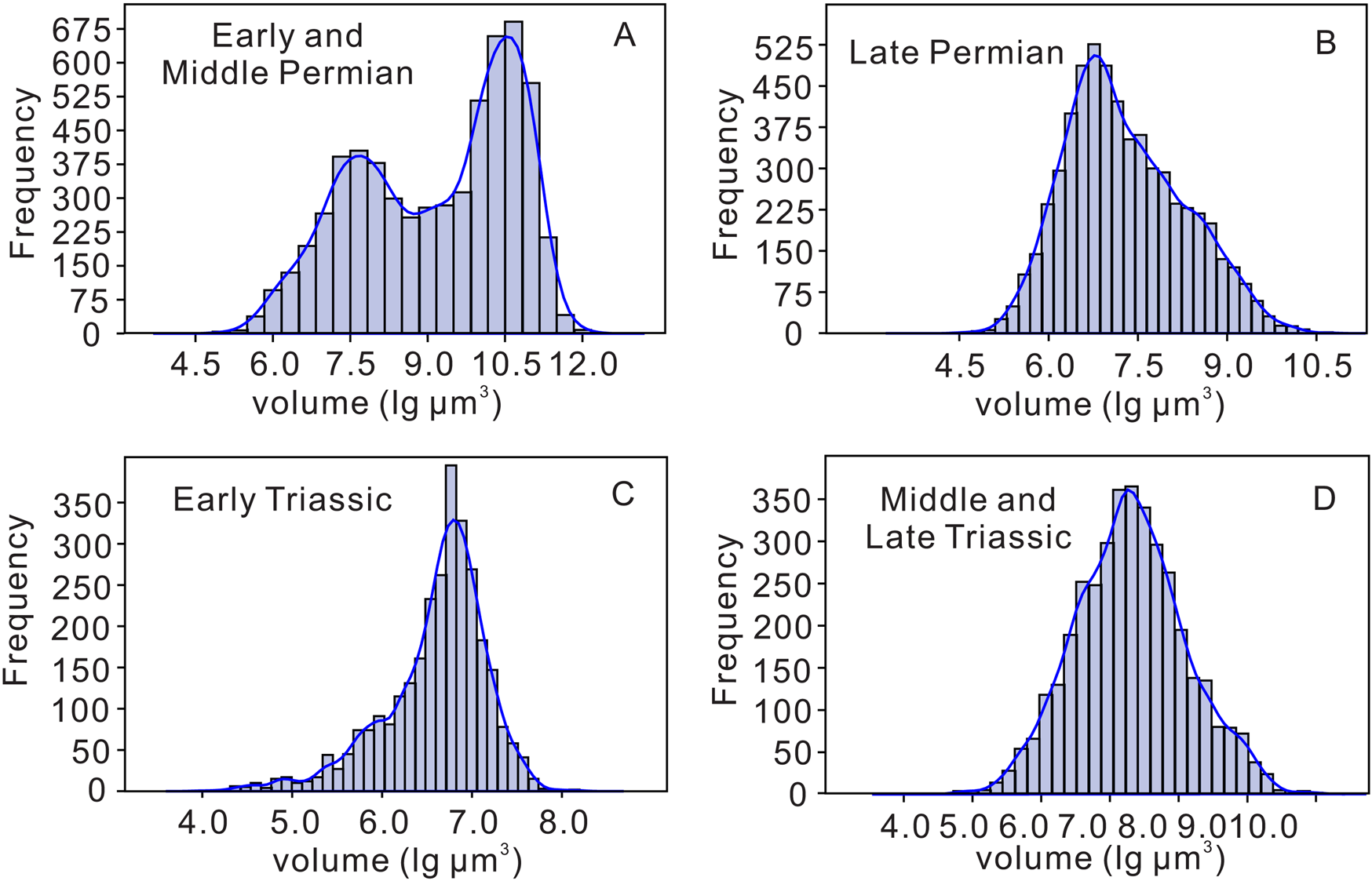
Figure 1. Histograms showing volumes of foraminifers (in lg μm3) in the database. A, Early and middle Permian; B, late Permian; C, Early Triassic; and D, Middle and Late Triassic.
Volume frequencies of foraminifers in the late Permian, Early Triassic, and Late Triassic specimens all conform to the normal distribution. Obviously, the test size of Triassic foraminifers is much smaller than that of Permian foraminifers. Volumes of Early Triassic foraminifers distribute between 4.5 lg μm3 and 7.5 lg μm3, and the dominant peak is 6.5–6.8 lg μm3 (Fig. 1C). That is, the volumes of foraminifers in the Early Triassic are the smallest in our study interval. In the Middle and Late Triassic, their size ranged from 5.0 lg μm3 to 10.0 lg μm3, with foraminifers having volumes from 7.0 lg μm3 to 8.0 lg μm3 being the most frequently occurring (Fig. 1D). This illustrates that the foraminifers increased in size during the Early–Middle Triassic intervals.
Foraminifer Size Variations
Variations in all foraminifer volumes (in lg μm3) during the Permian–Triassic intervals are shown in Figure 2. Figure 2A–C illustrate the test size variations for specimen-level mean values and genus-level mean and maximum values, respectively. All three figures show similar patterns, in which test size remained stable in the early Permian, and began to decrease from the middle Permian to the Early Triassic, then increase from the Middle Triassic, demonstrating that the total trend of test size variation is not sensitive to the size or taxonomic metric chosen. More interesting, the size change in our data shows trends similar to those identified in Payne et al.'s (Reference Payne, Jost, Wang and Skotheim2013) study of foraminiferal size evolution that includes almost 25,000 species and subspecies over the past 400 Myr. As mentioned earlier, we present subsequent analyses of size changes using the genus mean metric (Fig. 2B). Test size variations can be divided into four distinct intervals:
1. The early and middle Permian interval. The test size was the largest in both maximum (11.16 lg μm3 to 11.71 lg μm3) and mean (8.02 lg μm3 and 8.87 lg μm3) sizes throughout the whole study interval. Despite this, foraminifers decreased in mean size from the Asselian (8.79 lg μm3) to the Sakmarian (8.39 lg μm3), from the Kungurian (8.87 lg μm3) to the Roadian (8.31 lg μm3), and from the Wordian (8.62 lg μm3) to the Capitanian (8.02 lg μm3) (Table 2). These results are similar to those of Payne et al. (Reference Payne, Jost, Wang and Skotheim2013), who also found that test size in the early and middle Permian was the largest from the Devonian to the Neogene, with the mean volume of foraminifers being approximately 9 lg μm3.
2. The late Permian interval. There is a significant reduction in test size across the GLB. The mean test volume was 8.02 lg μm3 in the Capitanian before it decreased to 7.67 lg μm3 in the Wuchiapingian. Thus, Capitanian foraminifers were about 2.24 times larger than Wuchiapingian examples. In addition, the significant differences of all specimen mean values between adjacent stages have been tested with a t-test (Table 2), which clearly demonstrates that the test size declined sharply across the GLB. The mean volumes of foraminifer tests were relatively stable between the Wuchiapingian and the Changhsingian. Payne et al. (Reference Payne, Jost, Wang and Skotheim2013) observed a similar size reduction between the middle and late Permian, from mean volumes of approximately 9 lg μm3 in the Wordian and Capitanian to approximately 8 lg μm3 in the Wuchiapingian.
3. The late Permian to Early Triassic interval, including the transition across the PTB, sees the most significant size reduction in our entire database. The mean test volume was 7.53 lg μm3 for Changhsingian specimens, but this value dropped to 5.98 lg μm3 in the Induan. The t-test for specimen mean values indicates that the size decrease during this period was significant (p < 0.001). In addition, the change in mean during this period is the largest (−1.55 lg μm3) in the early Permian to Late Triassic interval (Table 2). Maximum and mean test volumes fluctuated slightly across the Induan/Olenekian boundary. The maximum and mean test sizes in Olenekian genera were 7.91 lg μm3 and 6.52 lg μm3, respectively. This is consistent with the significant mean size decrease across the PTB reported by Payne et al. (Reference Payne, Jost, Wang and Skotheim2013), who recorded mean test sizes in the Induan of approximately 6.8 lg μm3.
4. The Middle and Late Triassic interval. Foraminifers increased their maximum and mean sizes dramatically during the Olenekian and Anisian (the maximum and mean test volumes were 8.92 lg μm3 and 7.11 lg μm3, respectively). Overall, mean test volumes then remained relatively stable from the Anisian onward. These volume-change trends are identical to those of Payne et al. (Reference Payne, Jost, Wang and Skotheim2013), who noted that the mean size increased between the Early Triassic and the Middle Triassic and remained relatively stable in the Middle and Late Triassic (7.1 lg μm3).

Figure 2. Variations in volume (in lg μm3) of foraminifers from the beginning of the Permian to the end of the Triassic. A, mean test size variations for all specimens; B, mean test sizes of each genus; C, largest measured specimen of each genus. Abbreviations: As., Asselian; Sa., Sakmarian; Ar., Artinskian; Ku., Kungurian; Ro., Roadian; Wo., Wordian; Cap., Capitanian; Wu., Wuchiapingian; Ch., Changhsingian; In., Induan; Ol., Olenekian; An., Anisian; La., Ladinian; Car., Carnian; No., Norian; Rh., Rhaetian. The middle thick line and shaded areas represent the mean size of the foraminiferal volumes and the 95% confidence interval, respectively.
Size Variations in Foraminifer Suborders
We analyzed volume variations in nine foraminiferal suborders (Fig. 3). Four out of nine suborders survived during the Permian–Triassic intervals: Fusulinina, Textulariina, Miliolina, and Lagenina. In the Permian, the volumes of Fusulinina were largest in the early–middle Permian (>9.0 lg μm3), before they decreased significantly from the middle to late Permian. Thus, their mean test volume decreased from 9.40 lg μm3 in the Capitanian to 7.76 lg μm3 in the Wuchiapingian. The mean volume of Fusulinina tests in the Capitanian was 43.6 times larger than that in the Wuchiapingian. The mean values of Textulariina, Lagenina, and Miliolina were similar in the early–middle Permian, ranging from 5.93 lg μm3 to 8.12 lg μm3. All four suborders experienced a sharp reduction in mean volumes across the PTB (Fig. 3). For example, the mean volume of Fusulinina declined from 7.65 lg μm3 in the Changhsingian to 5.72 lg μm3 in the Induan. Thus, the mean volume of Fusulinina in the Changhsingian was 85.1 times greater than that in the Induan. The test size of these four suborders recovered between the Induan and Olenekian and increased significantly from the Early to Middle Triassic. In the Middle–Late Triassic, the volume of the nine extant suborders remained fairly stable (6.5–7.5 lg μm3) in mean value, with the exception of the Globigenina, whose test volumes fell from 6.87 lg μm3 in the Norian to 6.02 lg μm3 in the Rhaetian. However, the t-test was used to compare the mean value between the Norian and Rhaetian, suggesting that this size variation was not significant during this period (p = 0.518).

Figure 3. Trends in mean value of nine suborders of foraminifers from the beginning of the Permian through the end of the Triassic. Abbreviations are defined in Fig. 2. Each point represents the mean volume of specimens in a suborder within each stage. Solid lines represent continuous occurrences through time, dotted lines represent discontinuous occurrences, and shaded areas represent the 95% confidence intervals.
Fusulinina
To evaluate the different patterns in size variations experienced by the Fusulinina in contrast to Textulariina, Lagenina, and Miliolina (e.g., the major reductions in Fusulinina volumes across the GLB and PTB), we examined trends at the genus level within this suborder (Fig. 4A). During the early to middle Permian, the maximum volumes of Fusulinina exceeded 10.0 lg μm3, and the volumes of some genera even reached 11.0 lg μm3 (e.g., Verbeekina, Polydiexodina, and Pseudoschwagerina; Fig. 4A). During the late Permian, the maximum volumes of Fusulinina did not exceed 9.5 lg μm3. Many fusulinoidean fusulinid genera died out during the GLE, the victims of which included Verbeekina, Polydiexodina, and Codonofusiella. In the Early Triassic, the test size of Fusulinina dropped to <7.0 lg μm3 (Table 3), a function of the extinction of all remaining fusulinoidean fusulinids during the PTME. Some Permian genera (e.g., Polytaxis and Endoteba) that are absent in Early Triassic strata reappeared in the Middle–Late Triassic, so-called Lazarus taxa (Jablonski Reference Jablonski and Elliott1986). These Lazarus taxa led to an increase (Fig. 4A), but their tests were still smaller on average than they had been during the Permian.

Figure 4. Test size variations of Fusulinina from the beginning of the Permian through to the end of the Triassic. A, mean value trends of each genus. B,C, genus-level analysis of three component values (size-biased extinction, size-biased origination, and within-lineage evolution) across the GLB and PTB, respectively. Abbreviations are defined in Fig. 2. In A, the two thick solid lines in the middle represent the mean volume of fusulinoidean fusulinids and non-fusulinoidean fusulinids, respectively. The shaded areas represent the 95% confidence intervals. Fusulinoidea: 1, Verbeekina; 2, Polydiexodina; 3, Codonofusiella; 4, Pseudoschwagerina; 5, Parafusulina; 6, Pseudofusulina; 7, Rugosofusulina; 8, Quasifusulina; 9, Schwagerina; 10, Sumatrina; 11, Monodiexodina; 12, Sphaerulina; 13, Nankinella; 14, Staffella; 15, Yangchienia; 16, Pseudoendothyra; 17, Minojapanella; 18, Rauserella; 19, Reichelina; 20, Dunbarula; 21, Schubertella; 22, Cribrogenerina. Non-fusulinoidean fusulinids: 23, Polytaxis; 24, Climacammina; 25, Deckerella; 26, Globivalvulina; 27, Bradyina; 28, Palaeotextularia; 29, Endothyra; 30, Endothyranella; 31, Neoendothyra; 32, Dagmarita; 33, Endoteba; 34, Abadehella; 35, Tetrataxis; 36, Neotuberitina; 37, Endotriadella; 38, Earlandia; 39, Diplosphaerina. In B and C, stars denote extinction victims, circles denote genera that survived across the GLB and PTB, and squares denote new originations. The mean size of Capitanian genera was 8.651 lg μm3. For genera that survived into the Wuchiapingian, the mean size in the Capitanian was 7.992 lg μm3—smaller than the overall mean, so the extinction was size biased. The variation in mean size due to this size-biased extinction was 7.992 − 8.651 = −0.659 lg μm3. Of the surviving genera, their mean size in the Wuchiapingian was 7.835 lg μm3, and so the estimated change in size due to within-genus evolution is 7.835 − 7.992 = −0.157 lg μm3. The mean value of all Wuchiapingian Fusulinina was 7.706 lg μm3. Thus the change in mean size due to this size-biased origination was 7.706 − 7.835 = −0.129 lg μm3. This calculation method follows that of Rego et al. (Reference Rego, Wang, Altiner and Payne2012).
Table 3. Summary of volumes of tests (lg μm3) belonging to Fusulinina from the early Permian to the Late Triassic, including fusulinoidean fusulinids and non-fusulinoidean fusulinids. CI, confidence interval.

Figure 4A shows variations in volumes among fusulinoidean fusulinids and non-fusulinoidean fusulinids. Fusulinina with more than three occurrences in our database are represented. Our data set includes 39 genera in 16 families, of which fusulinoidean fusulinids make up 22 genera and non-fusulinoidean fusulinids make up 16 genera. Fusulinoidean fusulinids range in volume from 7.27 lg μm3 to 11.71 lg μm3. Nine genera survived the GLE: Sphaerulina, Nankinella, Pseudoendothyra, Staffella, Minojapanella, Rauserella, Dunbarula, Schubertella, and Reichelina. A volume reduction across the GLB resulted in mean volumes of fusulinoidean fusulinids decreasing from 9.84 lg μm3 in the Capitanian to 8.29 lg μm3 in the Wuchiapingian. All fusulinoidean fusulinids became extinct during the PTME. The test size of non-fusulinoidean fusulinids was smaller (<9.34 lg μm3), and their volumes were only modestly affected by the GLE. The larger genera Climacammina, Abadehella, Cribrogenerina, Deckerella, and Globivalvulina died out during the PTME, resulting in a further volume reduction across the PTB.
Figure 4B,C quantifies three modes of miniaturization of the Fusulinina across the GLB and PTB, and our methods follow those of Rego et al. (Reference Rego, Wang, Altiner and Payne2012). Figure 4B shows that the mean size of 49 Fusulinina genera was 8.651 lg μm3 in the Capitanian. Of these 49 genera, 33 died out across the GLB, and 16 existed into the Wuchiapingian. The mean value for the 16 survivors in the Capitanian was 7.99 lg μm3, which illustrates that larger genera were more likely to go extinct. This suggests that the test size change may have been due to size-biased extinction and the size change was 7.99 − 8.65 = −0.66 lg μm3. The mean size of the 16 surviving genera was 7.84 lg μm3 in the Wuchiapingian, and thus the size change due to within-genus trends is 7.84 − 7.99 = −0.15 lg μm3. In the Wuchiapingian, 11 genera originated, and the mean value of all Wuchiapingian Fusulinina was 7.71 lg μm3. Thus the size change due to size-biased origination is 7.71 − 7.84 = −0.13 lg μm3. Therefore, three modes can be considered the cause of size change across the GLE: size-biased extinction (−0.66 lg μm3), within-lineage change (−0.15 lg μm3), and size-biased origination (−0.13 lg μm3). All Changhsingian Fusulinina went extinct during the PTME, with the exception of Earlandia and Diplosphaerina (Fig. 4A). Figure 4C shows that the mean size of all Changhsingian Fusulinina was 8.06 lg μm3. The mean size of the surviving genera was 6.31 lg μm3 in the Changhsingian (Fig. 4A), and so the size reduction due to the size-biased extinction effect is 6.31 − 8.06 = −1.75 lg μm3. Two Fusulinina genera in the Induan are recorded in our data with a mean size of 5.49 lg μm3, meaning that the size decrease due to within-genus change is 5.49 − 6.31 = −0.82 lg μm3. Because no new genera of Fusulinina appeared in the Induan, the size change due to size-biased origination is 0. In summary, as for Fusulinina, size reduction following the GLE and PTME was driven mainly by the extinction of larger genera. Size change within surviving genera and the origination of new small genera could also have resulted in further size reduction.
Lagenina
The mean test volume of Permian Lagenina fluctuated over a narrow range (from 6.40 lg μm3 to 7.65 lg μm3; Fig. 3). The t-test for specimen means shows that the size reduction across the PTB was significant (p = 0.001; Fig. 5A). Only genera recorded in three or more stages are included in our analysis; thus Figure 5 includes 25 genera and 8 families. The genera Nodosinelloides, Lingulina, and Nodosaria exhibit size reduction across the PTB (e.g., the volume of Lingulina fell from 7.58 lg μm3 in the Changhsingian to 6.42 lg μm3 in the Induan). The mean test volume of the Lagenina began to increase from the Induan (5.78 lg μm3) to the Olenekian (6.07 lg μm3) (Table 4). More significant volume increases occurred between the Olenekian and the Anisian (6.91 lg μm3) (Table 4). Some new genera originated during the Anisian, such as Grillina and Astacolus. During the Middle–Late Triassic, some Lazarus genera also returned, such as Dentalina and Protonodosaria, and the range of mean test volumes was 6.91–7.55 lg μm3, similar to the volumes attained during the Permian (6.40–7.45 lg μm3).

Figure 5. Test size variations of Lagenina from the beginning of the Permian through to the end of the Triassic (25 genera in 8 families). A, Mean value trends of each genus. B,C, Genus-level analysis of three component values (size-biased extinction, size-biased origination, and within-lineage evolution) across the Guadalupian/Lopingian boundary and the Permian/Triassic boundary, respectively. Abbreviations are defined in Fig. 2. The calculation methods for B and C are listed in Fig. 4. Only genera occurring in three or more stages are included in this figure. Families are represented by different shapes. 1, Nodosinelloides; 2, Lingulina; 3, Dentalina; 4, Pseudoglandulina; 5, Nodosaria; 6, Pseudonodosaria; 7, Nodosinella; 8, Geinitzina; 9, Vervilleina; 10, Polarisella; 11, Pachyphloides; 12, Austrocolomia; 13, Protonodosaria; 14, Frondina; 15, Cryptoseptida; 16, Grillina; 17, Robuloides; 18, Rectostipulina; 19, Syzrania; 20, Tezaquina; 21, Pachyphloia; 22, Astacolus; 23, Lenticulina; 24, Marginulina; 25, Ichthyofrondina.
Table 4. Summary of test volumes (lg μm3) from the early Permian to the Late Triassic in the suborders Fusulinina, Lagenina, Miliolina, and Textulariina.

We further quantified three modes of size variation across the two extinction events (Fig. 5B,C). The mean size of all Capitanian Lagenina genera was 7.15 lg μm3, and of these, 9 genera survived to the Wuchiapingian. The survivors’ mean value in the Capitanian was 6.94 lg μm3. Thus the size change due to size-biased extinction effect is 6.94 − 7.15 = −0.21 lg μm3, while in the Wuchiapingian, the mean size of the surviving genera was 7.23 lg μm3, indicating that size change due to within-lineage change is 7.23 − 6.94 = 0.29 lg μm3. The mean size of all Wuchiapingian Lagenina was 7.37 lg μm3. Thus, the size change due to the biased-origination effect is 7.37 − 7.23 = 0.14 lg μm3. In summary, the size change across the GLB is −0.21 + 0.29 + 0.14 = 0.22 lg μm3, which confirms that there is no size decrease during this interval. Figure 5C shows that the mean size of 20 Lagenina genera was 7.11 lg μm3 in the Changhsingian, of these, 16 genera went extinct in the PTME. In the Changhsingian, the remaining 4 survivors’ mean value was 6.92 lg μm3. Thus the size reduction due to the size-biased extinction effect is 6.92 − 7.11 = −0.19 lg μm3. In the Induan, the survivors’ mean value was 5.84 lg μm3, so the size change due to within-lineage change is 5.84 − 6.92 = −1.08 lg μm3. In our data, no new Lagenina genera originated in the Induan, so the size change due to the biased origination effect is 0. In summary, the size reduction in the PTME was mainly due to within-lineage change. The extinction of large genera could also have resulted in further size reduction.
Miliolina
Figure 3 shows the mean size change of Miliolina specimens during the Permian–Triassic intervals. The mean size increased between the early and middle Permian. The t-test for the means of all specimens suggests that this size change was not significant (p = 1.000) in the middle Permian. A more significant volume reduction occurred across the PTB, probably as a result of the extinction of several genera or an adaptation to smaller sizes in order to survive. For example, Eolasiodiscus, Lasiodiscus, Multidiscus, and Neodiscus became extinct, while Rectocornuspira reduced its test volume during the PTME (Fig. 6A). A modest size increase occurred from the Induan to the Olenekian, and then the Miliolina increased in volume more significantly between the Early and Middle Triassic. This is mainly due to some new originations (Planiinvoluta and Ophthalmidium) and the reappearance of some Lazarus genera (Agathammina). The range of test volumes for the Miliolina reached 5.61–7.63 lg μm3 in the Middle to Late Triassic, still smaller than the test volumes of the Permian. Figure 6B,C shows three patterns of test size change in the GLE and PTME. There were 25 Miliolina genera in the Capitanian when mean size was 7.46 lg μm3. Of these, 10 genera survived to the Wuchiapingian, and the mean size of these genera in the Capitanian was 7.91 lg μm3. It is interesting that some small Miliolina genera disappeared across the GLB. Thus the size change due to extinction effect is 7.91 − 7.46 = 0.45 lg μm3. In the Wuchiapingian, the mean size of the survivors was 7.68 lg μm3, and thus the size change in the survivors is 7.68 − 7.91 = −0.23 lg μm3. The mean size of all Wuchiapingian Miliolina, including newly originating genera, was 7.60 lg μm3. Therefore, the size change due to biased origination effect is 7.60 − 7.68 = −0.08 lg μm3. In summary, the size change across the GLB is 0.45 + (−0.23) + (−0.08) = 0.14 lg μm3, which also illustrates that the size change during this interval was not particularly significant at the species level. In contrast, size change is apparent across the PTME. The mean size of all Changhsingian Miliolina was 7.59 lg μm3, of these, only 2 genera survived to the Induan. The survivors’ mean value was 7.13 lg μm3 in the Changhsingian. Thus, the size change due to size-biased extinction is 7.13 − 7.59 = −0.46 lg μm3. In the Induan, the survivors’ mean value was 6.09 lg μm3; thus the size change due to within-lineage change is 6.09 − 7.13 = −1.04 lg μm3. The mean size of all Miliolina in the Induan was 6.06 lg μm3. Therefore, the size change due to the biased origination effect is 6.06 − 6.09 = −0.03 lg μm3. The size decrease across the PTB is −0.46 + (−1.04) + (−0.03) = –1.53 lg μm3. In summary, there was no significant size change in the Miliolina across the GLE, whereas the decrease across the PTME is obvious and was mainly due to size-biased extinction and within-lineage reduction.

Figure 6. Test size variations of Miliolina from the beginning of the Permian through to the end of the Triassic (25 genera in 7 families). A, Mean value trends of each genus. B,C, Genus-level analysis of three component values (size-biased extinction, size-biased origination, and within-lineage evolution) across the Guadalupian/Lopingian boundary and the Permian/Triassic boundary, respectively. Abbreviations are defined in Fig. 2. The calculation methods for B and C are listed in Fig. 4. Only genera occurring in three or more stages are included in this figure. Families are represented by different shapes. 1, Rectocornuspira; 2, Calcitornella; 3, Cornuspira; 4, Meandrospira; 5, Planiinvoluta; 6, Calcivertella; 7, Cyclogyra; 8, Streblospira; 9, Agathammina; 10, Hemigordiopsis; 11, Hemigordius; 12, Orthovertella; 13, Neohemigordius; 14, Pseudovidalina; 15, Eolasiodiscus; 16, Lasiodiscus; 17, Xingshandiscus; 18, Multidiscus; 19, Neodiscus; 20, Ophthalmidium; 21, Gsollbergella; 22, Baisalina; 23, Nikitinella; 24, Pseudoglomospira; 25, Palaeonubecularia.
Textulariina
Figure 3 reveals that the mean test volumes of Permian Textulariina were stable. Size variations were minor, with test volumes ranging from 6.96 lg μm3 to 7.95 lg μm3. A notable volume reduction occurred across the PTB, with test volumes falling from 6.96 lg μm3 in the Changhsingian to 6.22 lg μm3 in the Induan. Textulariina began to increase in volume from the Induan to the Olenekian, driven primarily by the origination of genera such as Rectoglomospira and Palaeolituonella that increased in size significantly in the Olenekian. Figure 7 illustrates the genus trends in test volumes among the Textulariina and reveals that the range of mean test sizes among Textulariina was 6.22–7.21 lg μm3 in the Triassic, as large as they had been during the Permian.

Figure 7. Genus trends of Textulariina volumes from the beginning of the Permian through to the end of the Triassic. Abbreviations are defined in Fig. 2. Families are represented by different shapes. 1, Ammodiscus; 2, Ammovertella; 3, Glomospira; 4, Glomospirella; 5, Pilammina; 6, Rectoglomospira; 7, Tolypammina; 8, Turriglomina; 9, Turritellella; 10, Hyperammina; 11, Ammobaculites; 12, Kamurana; 13, Spiroplectammina; 14, Reophax; 15, Palaeolituonella; 16, Bigenerina; 17, Textularia; 18, Trochammina; 19, Verneuilinoides; 20, Duotaxis; 21, Gaudryina; 22, Gaudryinella.
Discussion
Sufficiency of Specimens
Sampling bias clearly has the potential to influence the range of foraminifer test volumes during each stage in our study. To evaluate the sampling sufficiency and demonstrate that our data are complete to the extent that they are representative of the volumes of all individuals in each stage, we conducted a rarefaction analysis (Fig. 8) that was first developed by Sanders (Reference Sanders1968). Rarefaction is used to compare the diversity of two samples based on similar sample sizes and can also be used to show whether the sample size is adequate (Raup Reference Raup1975). Figure 8 shows that further collecting is unlikely to add new genera, as each curve is approaching an asymptote.

Figure 8. Rarefaction curves (specimens vs. genera) of foraminifer test volumes for each stage. Abbreviations are defined in Fig. 2.
Size Variations across the GLB
The size reduction across the GLB has already been reported by previous studies (Isozaki et al. Reference Isozaki, Kawahata, Ota and Change2007; Bond et al. Reference Bond, Hilton, Wignall, Ali, Stevens, Sun and Lai2010b; Groves and Wang Reference Groves and Wang2013). Our study confirms that the reduction in test volumes across the GLB was a function of the extinction of larger fusulinoidean fusulinids during the GLE. The mean test volume of foraminifers decreased from 9.40 lg μm3 in the Capitanian to 7.76 lg μm3 in the Wuchiapingian (Fig. 3). Of these, the mean volume of fusulinoidean fusulinids was 9.84 lg μm3 in the Capitanian and 8.29 lg μm3 in the Wuchiapingian (Fig. 4). In addition, specimens belonging to the fusulinoidean fusulinids accounted for 53% of all foraminifers in the Capitanian, but only 19% in the Wuchiapingian. Non-fusulinoidean fusulinids, Miliolina, and Textulariina also saw a reduction in test volume between the Capitanian and Wuchiapingian, but only slightly. In contrast, Lagenina experienced a small increase in mean test volumes, from 7.17 lg μm3 in the Capitanian to 7.65 lg μm3 in the Wuchiapingian.
The Lilliput effect across the GLB can still be attributed to multiple drivers. Figure 4B has quantified three modes of Fusulinina size reduction in the GLE, that is, the selective extinction of large genera, within-lineage change, and the origination of new small genera, following the methods of Rego et al. (Reference Rego, Wang, Altiner and Payne2012). As discussed earlier, size decreased 8.651 − 7.992 = 0.945 lg μm3 from the Capitanian to the Wuchiapingian. Of the three modes of Fusulinina size reduction, size change owing to the size-biased extinction effect is −0.659 lg μm3, which means that the selective extinction of large genera was an important contributor to the size reduction across the GLE. However, it is also known that body size changes with environmental shift (Atkinson Reference Atkinson1994; Smith et al. Reference Smith, Betancourt and Brown1995). The miniaturization experienced by the Fusulinina might be linked to one or more of the following causes.
1. Emeishan Traps volcanism in southern China. The GLE has close temporal coincidence with the initial period of Emeishan volcanism (Wignall et al. Reference Wignall, Sun, Bond, Izon, Newton, Védrine, Widdowson, Ali, Lai and Jiang2009; Bond et al. Reference Bond, Wignall, Wang, Izon, Jiang, Lai, Sun, Newton, Shao and Védrine2010a). Large-scale volcanism can potentially destroy atmospheric ozone, resulting in excessive exposure to ultraviolet B among shallow-water taxa, with detrimental effects for photosynthetic taxa. Thus, keriothecal-walled fusulinaceans such as members of the Schwagerinidae and Neoschwagerinidae suffered preferential losses during the GLE, perhaps as a result of photosymbiont loss (Ross Reference Ross1972; Ota and Isozaki Reference Ota and Isozaki2006; Bond et al. Reference Bond, Wignall, Wang, Izon, Jiang, Lai, Sun, Newton, Shao and Védrine2010a). On the other hand, Zhang and Payne (Reference Zhang and Payne2012) illustrated that species in the keriothecal-walled families Verbeekidae, Neoschwagerinidae, and Schwagerinidae are much larger than members of the Schubertellidae, Staffellidae, and Ozawainellidae. However, smaller foraminifers are generally more likely to survive the environmental changes driven by a volcanism event because of their shorter generation times and comparatively lower energy needs (Song et al. Reference Song, Tong and Chen2011). In addition, Emeishan volcanogenic (and thermogenic) CO2 (Retallack Reference Retallack2002, Reference Retallack2005; Bond et al. Reference Bond, Hilton, Wignall, Ali, Stevens, Sun and Lai2010b; Bond and Grasby Reference Bond and Grasby2017) could have dissolved into seawater, resulting in its decreased pH value in the ocean, that is, oceanic acidification (Bond et al. Reference Bond, Hilton, Wignall, Ali, Stevens, Sun and Lai2010b), which would reduce calcification and growth rate of benthic calcareous foraminifers (Kuroyanagi et al. Reference Kuroyanagi, Kawahata, Suzuki, Fujita and Irie2009; Song et al. Reference Song, Tong and Chen2011). In short, the cessation of photosynthesis, lowered productivity, and acidification are all potential effects of Emeishan volcanism that might have driven the extinction of larger keriothecal-walled and calcareous foraminifers. Our study shows that the disappearance of larger fusulinoidean fusulinids and the miniaturization of survivors coincided with the emplacement of the Emeishan Traps (Figs. 4, 9), suggesting a causal link.

Figure 9. Summary of foraminifer test volumes (from this study), sea-surface temperatures, volcanic events, and oceanic anoxic events (OAEs) during the early Permian to the Late Triassic interval. The bars below represent the estimated original volumes of flood basalt provinces (Wignall Reference Wignall2001; Courtillot and Renne Reference Courtillot and Renne2003; Bond et al. Reference Bond, Hilton, Wignall, Ali, Stevens, Sun and Lai2010b). The long curve and short vertical lines below show global mean temperatures and 95% confidence intervals in °C, respectively (Song et al. Reference Song, Wignall, Song, Dai and Chu2019). The boxes above indicate OAEs (Isozaki Reference Isozaki1997; Wignall and Twitchett Reference Wignall and Twitchett2002; Clapham et al. Reference Clapham, Shen and Bottjer2009; Detian et al. Reference Detian, Liqin and Zhen2013; Song et al. Reference Song, Wignall, Song, Dai and Chu2019). Abbreviations are defined in Fig. 2. Additionally, ET, Early Triassic; GL, Guadalupian–Lopingian. The curve and shading represent mean test size of the foraminiferal specimens and the 95% confidence interval, respectively.
2. Oceanic anoxia, recorded locally across the GLB (Isozaki Reference Isozaki1997; Wignall et al. Reference Wignall, Bond, Kuwahara, Kakuwa, Newton and Poulton2010; Chen et al. Reference Chen, Joachimski, Sun, Shen and Lai2011; Bond et al. Reference Bond, Wignall, Joachimski, Sun, Savov, Grasby, Beauchamp and Blomeier2015, Reference Bond, Wignall and Grasby2020), is an oft-cited cause of species extinction in marine settings (Hallam and Wignall Reference Hallam and Wignall1997; Courtillot and Renne Reference Courtillot and Renne2003; Bond et al. Reference Bond, Wignall, Wang, Izon, Jiang, Lai, Sun, Newton, Shao and Védrine2010a, Reference Bond, Wignall, Joachimski, Sun, Savov, Grasby, Beauchamp and Blomeier2015), and oxygen deficiency is a potential driver of the Lilliput effect in foraminifers during the GLE. Most benthic invertebrates experience difficulties in secreting and retaining calcareous tests in oxygen-deprived environments (Rhoads and Morse Reference Rhoads and Morse1971). Therefore, larger calcareous foraminifers such as Fusulinina were more likely to die out in an anoxic-driven GLE scenario. On the other hand, foraminifers are very sensitive to variations in dissolved oxygen. Basov (Reference Basov1979) discovered that benthic foraminifers living in reduced oxygen settings tend to be smaller, usually with thinner and transparent walls and without sculpture.
3. Climate warming. It has been reported that a phase of global warming initiated near the GLB (Isozaki et al. Reference Isozaki, Kawahata, Ota and Change2007; Chen et al. Reference Chen, Joachimski, Sun, Shen and Lai2011, Reference Chen, Joachimski, Shen, Lambert, Lai, Wang, Chen and Yuan2013). Temperature is one of the most influential and pervasive environmental factors recognized as affecting body size (Angilletta et al. Reference Angilletta, Steury and Sears2004; Hunt and Roy Reference Hunt and Roy2006). The “temperature-size rule” invokes a negative correlation between temperature and body size (Atkinson and Sibly Reference Atkinson and Sibly1997; Hunt and Roy Reference Hunt and Roy2006; Atkinson et al. Reference Atkinson, Wignall, Morton and Aze2019), which is exhibited by many animals, including foraminifers (Lewis and Jenkins Reference Lewis and Jenkins1969; Bjørklund Reference Bjørklund1976; Schmidt et al. Reference Schmidt, Lazarus, Young and Kucera2006). First, oxygen solubility is lower in warmer waters, which would influence body size, as discussed earlier. Second, temperature can affect body size by changing the growth rate and the frequency of reproduction. For example, lower temperatures generally result in a slower growth rate and lower fecundity but a larger size at maturity (Angilletta et al. Reference Angilletta, Steury and Sears2004). Therefore, the predicted ~4°C warming across the GLB (Song et al. Reference Song, Wignall, Song, Dai and Chu2019) is also a potential driver of the Lilliput effect in foraminifers during the GLE (Fig. 9).
Size Variations across the PTB
The Lilliput effect has been observed in many organisms during the PTME (see references in the “Introduction”). More interestingly, the size change during the Permian–Triassic intervals shown in Figure 2A is in accordance with Payne et al.'s (Reference Payne, Jost, Wang and Skotheim2013) study of nearly 25,000 foraminiferal species and subspecies over the past 400 Myr, that is, the mean test size in the early and middle Permian was the largest at about 9 lg μm3. Mean size began to decrease from the middle Permian, and by the Induan, the mean test size was the smallest at about 6.8 lg μm3. Sizes then increased from the Induan to the Olenekian and became stable in the Middle and Late Triassic (7.2 lg μm3).
In our study, a size reduction is seen in all Lopingian foraminifers (i.e., Fusulinina, Lagenina, Miliolina, and Textulariina) across the PTB. In addition, all remaining fusulinoidean fusulinids became extinct during the PTME. Some larger non-fusulinoidean fusulinids also died out, such as Climacammina (Fig. 4), or had to reduce their volume (e.g., Glomospira; Fig. 7). Some new Early Triassic genera were very small and then became larger (e.g., Ophthalmidium; Fig. 6), which may be a function of the “Brobdingnag effect” introduced by Atkinson et al. (Reference Atkinson, Wignall, Morton and Aze2019).
With regard to the timing and cause of size reductions more generally, He et al. (Reference He, Shi, Feng, Campi, Gu, Bu, Peng and Meng2007) found that the Lilliput effect of brachiopod species appeared before the PTME, possibly as a result of regression, increased inflow of terrestrial material, and reduced productivity. Twitchett (Reference Twitchett2007) reported the Lilliput effect in both body and trace fossils in the aftermath of the PTME, driven by four factors (size-biased extinction, the new appearance of many small genera, the transitory disappearance of larger genera, and within-lineage size decreases) with origins in anoxia and food shortages. Luo et al. (Reference Luo, Lai, Shi, Jiang, Yin, Xie, Tong, Zhang, He and Wignall2008) demonstrated that the conodonts Hindeodus-Isarcicella underwent four distinct phases of size decrease across the PTB at Meishan, and two phases of size decrease in the earliest Triassic at Shangsi, possibly triggered by eustatic sea-level changes, hypoxic events, and carbon isotope fluctuations. Huttenlocker (Reference Huttenlocker2014) evaluated temporal distributions of therocephalian and cynodont therapsid body size during the middle Permian–Triassic intervals and found that the mean size in basal skull length of therocephalians decreased across both the GLB and PTB, probably in response to the ecological removal of large-bodied species. Chu et al. (Reference Chu, Tong, Song, Benton, Song, Yu, Qiu, Huang and Tian2015) described miniaturization in freshwater ostracods (0.4 lg μm3) during the PTME and invoked several stresses, consisting of global warming, hypoxia, and increased input of terrestrial materials following acid rain and wildfires. We consider that the causes of the Lilliput effect during the PTME can be summarized as follows:
1. Oceanic anoxia. Previous studies have demonstrated the development of super-anoxia during the PTB interval (Wignall and Twitchett Reference Wignall and Twitchett2002; Grice et al. Reference Grice, Cao, Love, Böttcher, Twitchett, Grosjean, Summons, Turgeon, Dunning and Jin2005; Bond and Wignall Reference Bond and Wignall2010; Brennecka et al. Reference Brennecka, Herrmann, Algeo and Anbar2011; Lau et al. Reference Lau, Maher, Altiner, Kelley, Kump, Lehrmann, Silva-Tamayo, Weaver, Yu and Payne2016; Li et al. Reference Li, Song, Algeo, Wignall, Dai and Woods2018), and such harmful conditions persisted in many areas throughout almost the whole Early Triassic, an interval of ~5 Myr (Wignall and Twitchett Reference Wignall and Twitchett2002; Grice et al. Reference Grice, Cao, Love, Böttcher, Twitchett, Grosjean, Summons, Turgeon, Dunning and Jin2005; Twitchett Reference Twitchett2007; Wignall et al. Reference Wignall, Bond, Kuwahara, Kakuwa, Newton and Poulton2010; Brennecka et al. Reference Brennecka, Herrmann, Algeo and Anbar2011; Song et al. Reference Song, Wignall, Tong, Bond, Song, Lai, Zhang, Wang and Chen2012, Reference Song, Wignall, Song, Dai and Chu2019; Tian et al. Reference Tian, Tong, Algeo, Song, Song, Chu, Lei and Bottjer2014; Zhang et al. Reference Zhang, Algeo, Romaniello, Cui, Zhao, Chen and Anbar2018). The development of oceanic anoxia closely coincided with the reduction in foraminiferal size seen in our data (Fig. 9), suggesting a causal link. In addition, our data reveal that the decline of foraminiferal size is significantly greater during the PTB interval than during the GLB interval, consistent with the wider extent and intensity of anoxia during the PTB interval.
2. Global warming, triggered by volcanogenic and thermogenic greenhouse gases from Siberian Traps volcanism and contemporaneous volcanic activity around the Paleotethys Ocean (Renne et al. Reference Renne, Black, Zichao, Richards and Basu1995; Svensen et al. Reference Svensen, Planke, Malthe-Sørenssen, Jamtveit, Myklebust, Eidem and Rey2004, Reference Svensen, Planke, Polozov, Schmidbauer, Corfu, Podladchikov and Jamtveit2009; Brand et al. Reference Brand, Posenato, Came, Affek, Angiolini, Azmy and Farabegoli2012; Joachimski et al. Reference Joachimski, Lai, Shen, Jiang, Luo, Chen, Chen and Sun2012; Yin and Song Reference Yin and Song2013; Majorowicz et al. Reference Majorowicz, Grasby, Safanda and Beauchamp2014). Oxygen isotope data from conodont apatite represent tropical sea-surface temperature warming of ~10°C during the PTB interval (Joachimski et al. Reference Joachimski, Lai, Shen, Jiang, Luo, Chen, Chen and Sun2012, Reference Joachimski, Alekseev, Grigoryan and Gatovsky2020). This hot climate lasted for much of the Early Triassic (Sun et al. Reference Sun, Joachimski, Wignall, Yan, Chen, Jiang, Wang and Lai2012; Romano et al. Reference Romano, Goudemand, Vennemann, Ware, Schneebelihermann, Hochuli, Brühwiler, Brinkmann and Bucher2013), and therefore temporally coincided with the Lilliput effect experienced by foraminifers (Fig. 9). Rapid warming is a likely driver of the Early Triassic Lilliput effect, and foraminiferal sizes only began to increase once the worst of the Early Triassic heat had abated.
We propose that volcanically induced global warming and anoxia were the principal drivers of the Lilliput effect in foraminifers across the GLB and the PTB. Our results do not preclude the role of other environmental elements in the size reduction of foraminifers, such as food shortage (Hallam Reference Hallam1965; Hunt and Roy Reference Hunt and Roy2006; Twitchett Reference Twitchett2007; Zhang et al. Reference Zhang, Shi, He, Wu, Lei, Zhang, Du, Yang, Yue and Xiao2016; Atkinson et al. Reference Atkinson, Wignall, Morton and Aze2019), sea-level change (Twitchett et al. Reference Twitchett, Feinberg, O'Connor, Alvarez and McCollum2005; He et al. Reference He, Shi, Feng, Campi, Gu, Bu, Peng and Meng2007; Sigurdsen and Hammer Reference Sigurdsen and Hammer2016; Atkinson et al. Reference Atkinson, Wignall, Morton and Aze2019), enhanced input of terrestrial materials (He et al. Reference He, Shi, Feng, Campi, Gu, Bu, Peng and Meng2007; Algeo and Twitchett Reference Algeo and Twitchett2010; Chu et al. Reference Chu, Tong, Song, Benton, Song, Yu, Qiu, Huang and Tian2015), and oceanic acidification (Kuroyanagi et al. Reference Kuroyanagi, Kawahata, Suzuki, Fujita and Irie2009; Song et al. Reference Song, Tong and Chen2011; Sephton et al. Reference Sephton, Jiao, Engel, Looy and Visscher2015). It is likely that many of these factors together contributed to the Lilliput effect of foraminifers and other organisms during these, and other mass extinction events.
Conclusions
Our study of 20,226 specimens in 464 genera, 98 families, and 9 suborders from 632 publications during the Permian–Triassic intervals has revealed that: (1) A decrease in foraminifer test volume (and by proxy, size) occurred during the two Permian extinction events (the GLE and PTME). (2) The main influence of the GLE was to reduce the test volumes of Fusulinina. Their size reduction was a function of the preferential extinction of taxa exhibiting gigantism, that is, the larger fusulinoidean fusulinids. The ecological impact of the GLE was modest, and this was clearly a less severe crisis than that of the PTME. (3) The PTME resulted in a major reduction in test volumes for all Permian suborders, that is, Fusulinina, Lagenina, Miliolina, and Textulariina. (4) The synergistic effects of volcanically induced global warming and anoxia are likely the ultimate drivers of the Lilliput effect recorded in our database.
Acknowledgments
We thank Y. Wang for his help in data collection; X. Dai for assistance with analyses; and E. Jia, X. Liu, and S. Jiang for useful discussions. This research was supported by the National Natural Science Foundation of China (41821001, 41622207, 41530104, 41661134047), the State Key R&D project of China (2016YFA0601100), the Strategic Priority Research Program of the Chinese Academy of Sciences (XDB26000000), and the National Mineral Rock and Fossil Specimens Resource Center, China. D.P.G.B. acknowledges support from the Natural Environment Research Council (grant no. NE/J01799X/1).


