


1. Introduction
In turbulent convection, persistent line plumes are the prominent coherent structures on the hot/cold convecting surfaces (Sparrow & Husar Reference Sparrow and Husar1969; Theerthan & Arakeri Reference Theerthan and Arakeri1994; Kitamura & Kimura Reference Kitamura and Kimura1995; Lewandowski et al. Reference Lewandowski, Radziemska, Buzuk and Bieszk2000). They contribute to most of the heat transport from the hot plate into the bulk fluid (Shishkina & Wagner Reference Shishkina and Wagner2008). The structure, the spatial and temporal distribution, and the dynamics of these line plumes hence predominantly determine the scaling of heat flux in turbulent convection (Puthenveettil et al. Reference Puthenveettil, Gunasegarane, Agrawal, Schmeling, Bosbach and Arakeri2011). Detection of these structures is therefore necessary to improve our understanding of the phenomenology of turbulent convection. In addition, detecting these structures from the flow field near hot surfaces is important in many applications such as designing surfaces with improved heat transfer characteristics in engineering, and estimating heat fluxes from the earth's surface. In the present paper, we present a novel kinematic approach to detect plumes from the velocity field near hot surfaces in turbulent convection.
Much of our knowledge about line plumes near the hot plate in turbulent convection comes from experimental visualisations, which implicitly use various plume detection criteria in their visualisation techniques. In electrochemical visualisations, plumes are identified as relatively dark regions where the concentration of a dark dye exceeds a visible threshold (Sparrow & Husar Reference Sparrow and Husar1969; Adrian, Ferreira & Boberg Reference Adrian, Ferreira and Boberg1986; Theerthan & Arakeri Reference Theerthan and Arakeri1998). In laser induced fluorescence techniques, however, plumes appear as relatively brighter fluorescing regions, owing to the relatively higher concentration of the fluorescent dye (Puthenveettil Reference Puthenveettil2004; Puthenveettil, Ananthakrishna & Arakeri Reference Puthenveettil, Ananthakrishna and Arakeri2005; Ramareddy & Puthenveettil Reference Ramareddy and Puthenveettil2011). Imaging flows laden with temperature sensitive liquid crystals detect plumes as regions where the temperature is locally high (Zhou & Xia Reference Zhou and Xia2010). Shadowgraphy detects plumes as regions with relatively low densities (Bosbach, Weiss & Ahlers Reference Bosbach, Weiss and Ahlers2012), while scattering of smoke particles by a laser sheet detects plumes as regions with relatively fewer particles (Puthenveettil et al. Reference Puthenveettil, Gunasegarane, Agrawal, Schmeling, Bosbach and Arakeri2011; Gunasegarane & Puthenveettil Reference Gunasegarane and Puthenveettil2014).
Characteristics of line plumes have also been studied in numerical simulations by using explicit criteria on the simulated velocity and temperature fields. Regions with
 \begin{equation} T'>c \sigma, \end{equation}
were identified as plumes by Gastine, Wicht & Aurnou (Reference Gastine, Wicht and Aurnou2015), where  $T'=T-\overline {\langle T\rangle }_A$ are the temperature fluctuations with $T$ being the instantaneous temperature and $\overline {\langle T\rangle }_A$ the temporally averaged spatial mean temperature, $\sigma =\sqrt {\overline {\langle T'^2 \rangle }_V}$ the volume averaged root mean square value of $T'$ and $c$ an arbitrary constant. Here, an overbar indicates averaging over time, subscript $A$ indicates area averaging over an entire horizontal plane and subscript $V$ indicates averaging over the entire domain volume. In other words, $\overline {\langle \ \rangle }_A$ and $\overline {\langle \rangle }_V$ represent spatiotemporal averaging over a horizontal plane and the entire domain volume, respectively. Another class of criteria used to detect plumes in numerical studies are based on the condition that the local vertical scalar flux in plumes is greater than that at other locations near the hot surface; an example is the criterion $wT'>0$ used by Schumacher (Reference Schumacher2009), where $w$ is the instantaneous vertical velocity. Criteria that combine temperature and flux-based conditions have also been used to detect plumes (Huang et al. Reference Huang2013); the same criterion has been used by Van der Poel et al. (Reference Van der Poel, Verzicco, Grossmann and Lohse2015) to study the statistics of these plumes. Shishkina & Wagner (Reference Shishkina and Wagner2008) detected plumes as regions having relatively high values of conditionally averaged (on temperature) values of thermal dissipation rates, after examining similar values of vertical velocity, absolute value of horizontal velocity, heat flux and vertical and horizontal vorticity components. As is evident even from this short discussion, there is no consensus on how to identify plumes near hot surfaces in turbulent convection. Furthermore, the relation between the many available criteria, and hence the regions identified by them, remains unclear.
All the aforementioned studies detect plumes as regions above a threshold on a scalar concentration field, or on the heat flux field, based on the understanding that plumes have higher values of scalar concentration or local heat flux, compared with the ambient. However, plumes are not just scalar structures; they also have associated velocity fields. The spatial extent of these velocity structures will be different from those of the scalar structures for Prandtl numbers,  $Pr \ne 1$. For the most commonly occurring $Pr>1$ cases in liquids, the velocity structures will be of larger spatial extents than the associated high scalar concentration regions. Detecting plumes based on their scalar signatures alone is hence unlikely to capture their entire extent since, at $Pr>1$, they have thinner, higher scalar concentration regions surrounded by thicker, higher vertical velocity regions (Gebhart, Pera & Schorr Reference Gebhart, Pera and Schorr1970). Further, scalar fields are quite hard to obtain in experimental studies; it is even harder to obtain scalar fields simultaneously with the velocity fields in experiments, as necessary for detecting plumes from flux-based criteria (Schumacher Reference Schumacher2009). In contrast, spatial velocity fields are easily obtained from particle imaging velocimetry (PIV); a velocity-based, kinematic criterion to detect plumes would then be immensely useful in such studies to shed more light on plume dynamics and the associated heat transport.
A critical gap in the understanding of transport due to line plumes is the effect of the large-scale flow (or large-scale circulation) on plumes, and the effect plumes in turn have on the large-scale flow (LSF). A velocity-based detection scheme of these plumes will help in bridging this gap, and delineate the plumes, the large-scale flow and their interaction. No such rigorous velocity-based criteria for separating plumes from the ambient and the boundary layers near the plate in turbulent convection are available. In contrast, in shear turbulence, sophisticated kinematic schemes such as  $Q$-criterion (Hunt, Wray & Moin Reference Hunt, Wray and Moin1988), $\lambda _2$ criterion (Jeong & Hussain Reference Jeong and Hussain1995) and the swirling strength ( $\lambda _{ci}$) method (Zhou et al. Reference Zhou, Adrian, Balachandar and Kendall1999), are used to detect coherent structures in near-wall regions. Even though these criteria detect coherent vortices, and not plumes, they have been applied in turbulent convection to detect plumes (De, Eswaran & Mishra Reference De, Eswaran and Mishra2018). Such applications are, however, unlikely to be appropriate since, due to their entraining nature, plumes are attracting, rather than vortical, structures. Attracting structures that underlie material transport in flows of varying complexity have previously been defined, identified and studied using the rigorous kinematic framework of Lagrangian coherent structures (LCS) (Haller Reference Haller2015); the framework has revealed hidden structures that organise complex tracer patterns in a wide range of natural and laboratory flows. While the scalar species present in excess in plumes, namely temperature/concentration, are diffusive and also actively influence the flow field, Mensa et al. (Reference Mensa, Özgökmen, Poje and Imberger2015) have shown that patterns in such scalar fields are still strongly correlated with the structures governing material transport in the flow. Specifically, they showed that convective plumes in the ocean boundary layer with a weak wind forcing drive the clustering of tracers. A velocity-based kinematic criterion to detect plumes would then clarify this connection of plumes structures with LCS, and hence the advective transport of active, diffusive scalars.
In this study, we propose a novel criterion to extract line plumes from the horizontal velocity field in a plane parallel and close to the hot plate in turbulent convection. The proposed criterion of negative values of horizontal divergence of the horizontal velocity field is shown to detect plume regions for the range of Rayleigh numbers  $5.5\times 10^5\le Ra\le 1.2\times 10^9$ and $1\le Pr\le 10$ reasonably well. This criterion, which is simple to compute from only the spatial distribution of horizontal velocity components in a plane parallel and close to the plate, does not need any arbitrary threshold value that varies from flow to flow. In § 2, we describe the experiments and simulations used to obtain the velocity fields in a horizontal plane close to the hot plate in Rayleigh–Bénard convection (RBC). The proposed horizontal divergence criterion is then motivated from the theoretical similarity solutions of plumes and boundary layers in § 3.1. Examining the deformation of a fluid element close to the hot plate, we then show in § 3.2 that regions with dominant negative eigenvalues of the strain rate are likely to be plumes. In § 3.3, we invoke the definition of attracting LCS in the instantaneous limit, and subsequently the tendency of plumes to act as attracting LCS, to show that plumes are regions of attracting LCS that do not have stronger, repulsive LCS overlying on them; this understanding then justifies the horizontal divergence criterion. Four types of regions in the flow field near the hot plate are then identified based on the distribution of eigenvalues of the strain rate in § 3.4 to show the influence of shear due to the large-scale flow. The characteristics of the regions detected by the criterion are compared with the theoretical estimates of these regions, and with the results of applying various other available criteria for plume detection in § 4. The main conclusions of the paper are summarised in § 5.
2. Experiments and simulations
We conduct laboratory experiments to obtain the spatiotemporal velocity fields in a horizontal plane close to the hot surface in RBC, while numerical simulations are performed to obtain velocity and temperature fields simultaneously and explore a wider range of  $Pr$ than in the experiments.
2.1. Experiments
2.1.1. Apparatus
Velocity field measurements were conducted for steady, temperature-driven convection in water in an RBC cell of cross-sectional area  $300\times 300$ mm $^2$, as shown in figure 1(a). The bottom hot copper plate, painted black to prevent reflection of light from its surface, was kept above a thin glass plate, which was above two aluminium plates that had a nichrome wire heater sandwiched between them. A constant heat flux was provided by a Variac connected to the wire heater. The heat flux was estimated by measuring the temperature difference $(T_1-T_2)$ across the glass plate in the heater assembly using T-type thermocouples. The sides and the bottom of the convection cell were insulated. The top cold plate, made of glass, was maintained at a constant temperature by circulating refrigerated water in a glass compartment above the plate. A water filled glass prism was fixed on top of this glass compartment to rectify the radial distortions in stereoscopic imaging. The vertical location of the cold plate assembly – which included the cold plate, the glass compartment and the glass prism – could be adjusted. The temperature difference between the bottom plate ( $T_B$) and the top plate ( $T_T$), $\Delta T=T_B-T_T$, was measured using thermocouples touching the hot copper plate at the bottom and the cold glass plate at the top. Measurements were made only after a steady state was attained after around three hours, when $\Delta T$ remained a constant, as monitored by a data logger (Agilent, model 34970A). The water layer height $H$ and the constant heat flux through the bottom copper plate were changed to vary the Rayleigh number $Ra=g\beta \Delta T H^3/\nu \alpha$, where $g$ is the gravitational acceleration, $\beta$ the coefficient of thermal expansion, $\nu$ the kinematic viscosity and $\alpha$ the thermal diffusivity. The values of $H$,
$H$,  $\Delta T$ and the corresponding estimated values of $Ra$ and Prandtl number ( $Pr = \nu /\alpha$) are shown in table 1. Figure 1(b) shows an example of the pattern of line plumes observed on the hot surface, obtained by electrochemical dye visualisation (Baker Reference Baker1966) at $Ra= 8.26\times 10^6$ and $Pr= 6$ (Gunasegarane Reference Gunasegarane2015).

Figure 1. (a) Schematic of the experimental set-up. (b) Top view of the line plumes at  $Ra=8.26\times 10^6$ and $Pr=6$ detected by electrochemical dye visualisation (Gunasegarane Reference Gunasegarane2015). See Movie 1 available at in the supplementary movies for corresponding velocity field in RBC experiments.
Table 1. Values of experimental parameters, length scales and PIV parameters. Physical properties of the fluid were estimated at  $T_b$, where $T_b$ is the temperature of the bulk fluid. For PIV, one side of the square interrogation window $D_I$ was equal to 32 pixels and the overlap was equal to $50\,\%$. Vertical velocity at the centreline of a plume, estimated from the similarity solutions of Gebhart et al. (Reference Gebhart, Pera and Schorr1970), is shown as $w_{pc}$. Here $V_{sh}$ is the large-scale flow velocity given by (3.25).

2.1.2. Velocity measurements
Velocity fields in a horizontal ( $x$–
$x$– $y$) plane, parallel and close to the hot copper plate at the bottom, were obtained by stereo PIV at different $Ra$. The height $h_m$ of the measurement plane above the hot plate was within the Prandtl–Blasius velocity boundary layer thickness ( $\delta _{pb}$) and within the natural convection velocity boundary layer thickness ( $\delta _{nc}$), as estimated from Ahlers, Grossmann & Lohse (Reference Ahlers, Grossmann and Lohse2009) and Puthenveettil et al. (Reference Puthenveettil, Gunasegarane, Agrawal, Schmeling, Bosbach and Arakeri2011) (see table 1). The flow was seeded with polyamide spheres (mean diameter $d_p=55\,\mathrm {\mu }$m and density $\rho _p=1.012$ g cm $^{-3}$), which were illuminated by a laser sheet of maximum thickness $h_l=1$ mm from an Nd:YAG laser (Litron, 100 mJ pulse $^{-1}$). The value of the particle Stokes number, which represents the ratio between particle relaxation time and the characteristic time scale of the flow, was less than $0.00415$; the particles hence followed the flow. Two $1024\times 1280$ pixels Imager Pro cameras (LaVision GmbH), with Scheimpflug adapters, oriented at $32^\circ$ with the vertical, were used to capture the particle images in a single pulse, single frame mode. The depth of field of imaging was around $2$ mm, greater than $h_l$. Imaging was done at the centre of the plate so that image areas $A_i$ had at least eight to $12$ plumes; the values of $A_i$ are shown in table 1. The laser pulse separation $\Delta t$ was chosen such that the largest out-of-plane particle displacement was not more than a quarter of the laser sheet thickness. The maximum in-plane particle displacement over this $\Delta t$ was around 10 pixels at each $Ra$. The particle images were filtered using a high pass filter to remove noise and to make the varying background uniform. A stereo cross-correlation method was used to evaluate the three components of the velocity field in a plane (2D3C vector field).
The size of the interrogation window was chosen so that a minimum of three velocity vectors were present within the plume thickness  $t_p$ at any $Ra$; values of $t_p$, estimated from the similarity solutions for line plumes (Gebhart et al. Reference Gebhart, Pera and Schorr1970), are given in table 1. The corresponding spatial resolution of velocity vectors $L_v$ at different $Ra$ are shown in table 1; the number of vectors in $t_p$ varied from approximately seven at the lowest $Ra$ to approximately three at the highest $Ra$. The size of the interrogation window was also limited by the condition that the displacement due to the largest velocity in the horizontal plane was less than a quarter of the size of the interrogation window and that a minimum of 10 particles were present in the interrogation window for robustness of correlation. The bias errors were reduced by using a multipass adaptive window cross-correlation technique. Subpixel interpolation ensured that the peak lock value was less than $0.1$, the acceptable limit of peak locking effect. Spurious vectors were removed by applying a median filter of $3\times 3$ pixel neighbourhood with interpolated vectors replacing the spurious vectors. A third-order polynomial fit was applied to the final vector field to ensure accurate calculation of the velocity derivatives. Such smoothed vector fields were used for the calculation of spatial derivatives.
2.2. Numerical simulations
The non-dimensional governing equations under the Boussinesq, incompressible approximation are
 \begin{gather} \boldsymbol{\nabla}^*\boldsymbol{\cdot} \boldsymbol{V}^*=0, \end{gather}
 \begin{gather} \frac{{\rm D}\boldsymbol{V}^*}{{\rm D}t^*} ={-}\boldsymbol{\nabla}^*P^*+ \left( \sqrt{\frac{Pr}{Ra}}\right) {\nabla}^*{^2} \boldsymbol{V}^* + T^* \boldsymbol{e_z}, \end{gather}
 \begin{gather} \frac{{\rm D} T^*}{{\rm D}t^*}=\frac{1}{ \sqrt{Ra\,Pr}}{\nabla}^*{^2} T^*, \end{gather}
where the lengths are normalised by  $H$, time by $H/u_f$, $\boldsymbol {V}^*$ is the dimensionless velocity field obtained by normalising by the free-fall velocity $u_f=\sqrt {g\beta \Delta T H}$, $T^*=(T-T_C)/\Delta T$ and $\boldsymbol {e_z}$ is the unit vector in the $z$ direction. Here $T^*$ varies from a constant value of one at the bottom surface to zero at the top plate. The computations were done for a cylindrical domain with adiabatic sidewalls and an aspect ratio, $\varGamma = D/H$ of one, for $Ra = 2\times 10^7, 2\times 10^8$ and $Pr=1,\, 4.96, 10$.
The numerical schemes described in Verzicco & Camussi (Reference Verzicco and Camussi2003) are used for solving (2.1)–(2.3). In brief, we use a second-order finite difference scheme discretised on a staggered mesh in a cylindrical domain. The time integration is done using an explicit third-order Runge–Kutta scheme (Verzicco & Camussi Reference Verzicco and Camussi1997; Verzicco & Orlandi Reference Verzicco and Orlandi1996) for nonlinear terms, and implicit Crank–Nicholson scheme for the linear terms, as described in the fractional step method discussed in Kim & Moin (Reference Kim and Moin1985). The discretised equations are solved by a fractional-step procedure. The pressure equation is inverted using trigonometric expansion in the azimuthal direction and FISHPACK package (Swartzrauber Reference Swartzrauber1974) in the other two directions. The grid size  $N_{\theta }\times N_r \times N_z$ used in the simulations is $513\times 129\times 385$. This ensures $33$ grid points in the thermal boundary layer for $(Ra,Pr)=(2\times 10^8,10)$, satisfying the criterion suggested by Shishkina et al. (Reference Shishkina, Stevens, Grossmann and Lohse2010). The maximum grid size in the vertical direction is $0.006$ and the Courant–Friedrichs–Lewy number was fixed at ${\rm CFL}=0.5$ with a maximum time step ${\rm d}t=0.0331$.
3. Kinematic approach to separating plumes from boundary layers
Any criterion to detect coherent structures near the hot plate in turbulent convection should reproduce, both qualitatively and quantitatively, the complex, connected structure of line plumes similar to that in figure 1(b). Even though these plume structures appear random in space and time, successful scaling law predictions for the mean spacings between such line plumes (Theerthan & Arakeri Reference Theerthan and Arakeri1998; Puthenveettil & Arakeri Reference Puthenveettil and Arakeri2005), their total lengths (Puthenveettil et al. Reference Puthenveettil, Gunasegarane, Agrawal, Schmeling, Bosbach and Arakeri2011), and their mean dynamics (Gunasegarane & Puthenveettil Reference Gunasegarane and Puthenveettil2014) have all been obtained. Such scaling laws use the similarity solutions of steady two-dimensional (2D) laminar plumes originating from line sources of heat (Gebhart et al. Reference Gebhart, Pera and Schorr1970) and those of steady 2D laminar natural convection boundary layers (Rotem & Claassen Reference Rotem and Claassen1969; Pera & Gebhart Reference Pera and Gebhart1973) feeding these plumes. It therefore appears that plumes near the hot plate in turbulent convection can be approximated as steady 2D laminar plumes originating from line sources of heat. As a result, we first analyse the theoretical velocity fields associated with such an idealised plume, and the boundary layer feeding the plume. This analysis leads us to a possible kinematic condition to separate plumes from boundary layers. A schematic depicting the division of the flow into plume, boundary layer and bulk regions is shown in figure 2(a).

Figure 2. (a) Schematic of the side view of the typical evolution of the shape of a fluid element along its trajectory near the hot plate in RBC. The unhatched region indicates the plume along with its vertical velocity profiles, the 45 $^\circ$ hatched region indicates boundary layers along with its horizontal velocity profiles and the 135 $^\circ$ hatched region indicates the bulk fluid. The horizontal dashed line indicates the location of measurement of the velocity fields. Locations 1, 2 and 3 on a pathline show the shape of a spherical fluid element in the bulk, boundary layer and the plume, respectively. (b) Variation of the dimensionless vertical velocity, horizontal velocity and the horizontal gradient of the horizontal velocity across a plume and a boundary layer, calculated from the similarity solutions of Gebhart et al. (Reference Gebhart, Pera and Schorr1970) and Pera & Gebhart (Reference Pera and Gebhart1973), respectively. Solid lines show the plume solutions while the dashed lines show the boundary layer solutions. Here $\circ,\, u z/\nu \sqrt {Gr_z}$; $+,\, w z/\nu \sqrt {Gr_z}$; lines with no markers show $(\partial u/\partial x)z^2/ \nu \sqrt {Gr_z}$.
3.1. Theoretical velocity distributions
3.1.1. Plume
For a steady, 2D, laminar line plume, shown as the unhatched region in the schematic in figure 2(a), denoting the plume variables by the subscript  $p$, the dimensional horizontal and vertical velocity profiles are (Gebhart et al. Reference Gebhart, Pera and Schorr1970)
 \begin{gather} u_p(z,\eta_p)={-}4^{3/4}\frac{\nu}{z}Gr_z^{1/4}\left(\frac{3}{5}f_p(\eta_p)-\frac{2}{5}\eta_p f_p'(\eta_p) \right), \end{gather}
 \begin{gather} w_p(z,\eta_p)=4^{1/5}\left(\frac{g\beta Q_p}{C_p I}\right)^{2/5}\left(\frac{z}{\mu \rho}\right)^{1/5} f_p'(\eta_p). \end{gather}
Here,  $f_p(\eta _p)$ is the dimensionless stream function obtained as the numerical solution of the self-similar plume equations; an approximation of $f_p$ is given in Appendix A (A1). In (3.1) and (3.2), a prime denotes differentiation with respect to the similarity variable $\eta _p$, defined as
 \begin{equation} \eta_p=\frac{x_p}{z}\left(\frac{Gr_z}{4}\right)^{1/4}, \end{equation}
where,  $x_p$ is the horizontal distance from the plume centreline and $Gr_z=g\beta (T_0-T_\infty )z^3/\nu ^2$ is the Grashoff number based on the vertical distance $z$ from the hot plate. Here, $T_0$ and $T_\infty$ denote the temperatures at the plume centreline and the ambient, respectively. In (3.2), the heat flux per unit length of the line source is
 \begin{equation} Q_p=4^{3/4} (g \beta)^{1/4}\sqrt{\rho\mu} IC_pN^{5/4}, \end{equation}
where  $N$ is a constant, $C_p$ is the specific heat at constant pressure and $I =\int _{-\infty }^\infty f_p'\phi \,{\rm d}\eta _p$, with $\phi =(T-T_\infty )/(T_0-T_\infty )$ and
 \begin{equation} T_0-T_\infty=Nz^{{-}3/5}. \end{equation}
Using (3.4) and (3.5) in (3.2) and (3.1), we obtain the dimensionless horizontal and vertical velocities within the plume as
 \begin{gather} u_p^*= \frac{u_p}{\nu\sqrt{Gr_z}/z} ={-}4^{3/4}Gr_z^{{-}1/4}\left(\frac{3}{5}f_p-\frac{2}{5}\eta_pf_p' \right), \end{gather}
 \begin{gather}w_p^*=\frac{w_p}{\nu\sqrt{Gr_z}/z}=2f_p', \end{gather}
where  $f_p$ and $f_p'$ are given by (A1) and (A2).
Figure 2(b) shows the profiles of dimensionless horizontal and vertical velocities, (3.6) and (3.7), across a plume. The plume has an upward vertical velocity, which has a maximum at the centreline and reaches zero at its edge. Differentiating (3.7) with respect to  $z$, we obtain the dimensionless vertical gradient of vertical velocity as
 \begin{equation} \frac{\partial w_p^*}{\partial z^*}= \frac{\partial w_p/\partial z}{\nu\sqrt{Gr_z}/z^2}=\frac{2}{5}\left( f_p'-2\eta_p f_p''\right). \end{equation}
From (3.8), we see that the plume region, shown as the unhatched region in figure 2(a), has a positive vertical spatial acceleration,  $\partial w_p/\partial z\sim 1/z^{4/5}$; the positive vertical acceleration increases as we approach the hot plate. Simultaneously, owing to continuity, $\partial u_p/\partial x_p=-\partial w_p/\partial z\sim -1/z^{4/5}$ is a negative quantity. With $u_p$ being zero at the plume centreline, the horizontal velocities within the plumes are negative and decrease in magnitude as we approach the centre of the plumes from its edges. In summary, $\partial w_p/\partial z>0$ and ${\partial u_p/\partial x_p<0}$ in the unhatched plume region of figure 2.
3.1.2. Boundary layer
For a steady, 2D natural convection boundary layer, shown as the  $45^\circ$ hatched regions in figure 2(a), the horizontal and vertical velocity profiles are (Pera & Gebhart Reference Pera and Gebhart1973)
 \begin{align} u_b&=5^{3/5}\frac{\nu}{x_b}Gr_x^{2/5}f_b'\quad{\rm and} \end{align}
 \begin{align} w_b&={-}\frac{\nu}{x_b}\left(\frac{Gr_x}{5}\right)^{1/5}\left(3f_b-2\eta_bf_b'\right), \end{align}
where the subscript  $b$ denotes boundary layer variables. Here, $Gr_x=g\beta (T-T_\infty ) x_b^3/\nu ^2$ is the Grashoff number based on the horizontal distance $x_b$ within the boundary layer. Here $x_b = 0$ is the leading edge from where the boundary layer forms, and the boundary layer thickens as $x_b$ increases and we approach the plume. The dimensionless stream function $f_b(\eta _b)=\psi _b/(5\nu (Gr_x/5)^{1/5})$, an approximation of which is given by (A3), with $\psi _b$ being the stream function, and a prime denotes differentiation with respect to the boundary layer similarity variable,
 \begin{equation} \eta_b=\frac{z}{x_b}\left(\frac{Gr_x}{5}\right)^{1/5}. \end{equation}
Using (3.3), (3.11) can be rewritten in terms of  $\eta _p$ as
 \begin{equation} \eta_b=\frac{1}{4^{1/10}5^{1/5}}\frac{Gr_z^{3/10}}{\eta_{p}^{2/5}}. \end{equation}
Rewriting (3.9) and (3.10) in dimensionless form using (3.12), we obtain the dimensionless horizontal and vertical velocities as
 $$\begin{gather} u_b^*=\frac{u_b}{\nu \sqrt{Gr_z}/z}=5^{3/5}4^{1/20}\frac{\eta_p^{1/5}}{Gr_z^{3/20}}f_b', \end{gather}$$
 $$\begin{gather}w_b^*=\frac{w_b}{\nu \sqrt{Gr_z}/z}=\frac{1}{5^{1/5}4^{1/10}}\frac{1}{\eta_p^{2/5}Gr_z^{1/5}}, \left(3f_b-2\eta_bf_b' \right), \end{gather}$$
where  $f_b$ and $f_b'$ are given by (A3) and (A4).
The variations given by (3.13) and (3.14) along the boundary layer that feeds the plume at its base, as shown schematically in figure 2(a), are shown in figure 2(b). To plot (3.13) and (3.14) in figure 2(b), we write (A3) and (A4) in terms of  $\eta _p$ using (3.12). Figure 2(b) shows that the horizontal velocity (towards the plume) inside the boundary layer region increases as we approach the plume, as also shown schematically in figure 2(a). From (3.9),
 \begin{equation} \frac{\partial u_b}{\partial x_b} =\frac{1}{5^{2/5}} \frac{\nu }{x_b^2} Gr_x^{2/5} \left(f_b'-2\eta_bf_b''\right) \end{equation}
is identified as a positive quantity, whose value decreases as  $x_b^{-4/5}$ as we approach the plume from the leading edge of the boundary layer. This increase in horizontal velocity along the boundary layer occurs since the driving horizontal pressure gradient due to the density difference, $\Delta p \approx \rho g \beta \Delta T \delta _{nc}$, increases with increase in boundary layer thickness as we approach the plume. As discussed in § 3.1.1, inside the plume, the horizontal velocity decreases towards its centreline. Figure 2(b) shows that the boundary layer has a small vertical downward velocity far away from its leading edge, which increases to appreciable values closer to its leading edge; these boundary layers entrain ambient fluid into them. From (3.15), by continuity, $\partial w_b/\partial z\sim -x_b^{-4/5}$, a negative quantity. Hence, as shown schematically in the boundary layer regions in figure 2(a), for the regions within the boundary layers feeding the plumes on either side at the bottom of the plumes, $\partial u_b/\partial x_b >0$ and $\partial w_b/\partial z<0$.
In the ambient/bulk fluid region above the boundary layers, rising plumes cause flows due to the ambient fluid being entrained into them. Such entrainment flows are expected to have  $\partial w/\partial z<0$ since the large-scale flow in the bulk is of an order higher in magnitude than the entrainment flows into the plumes and the boundary layers (Gunasegarane & Puthenveettil Reference Gunasegarane and Puthenveettil2014). Further, the kinematic blocking due to the presence of the bottom plate also slows down the downward vertical velocities as we approach the bottom plate. Hence, $\partial w/\partial z$ is expected to be negative in the regions shown as bulk in figure 2(a). In addition, the presence of plumes also results in increasing horizontal velocities in the bulk ( $\partial u/\partial x>0$) due to the entrainment, as shown by the horizontal arrows in the bulk region in figure 2(a). We then see that the flow in and around a 2D laminar plume and a 2D laminar boundary layer feeding it at the bottom separates into two regions, viz. (i) the plumes where $\partial w/\partial z>0$ and $\partial u/\partial x<0$ and (ii) the bulk and the boundary layers where $\partial w/\partial z<0$ and $\partial u/\partial x>0$; these two regions are shown as the unhatched and the hatched regions, respectively, in figure 2(a). To separate the plumes from the boundary layers and the bulk in such flows, we then need a criterion that distinguishes the $\partial w/\partial z>0$, $\partial u/\partial x<0$ regions as plumes from the $\partial w/\partial z<0$, $\partial u/\partial x>0$ regions as bulk or boundary layers.
Extending the above considerations to a three-dimensional (3D) flow, the horizontal, 2D divergence of the horizontal velocity components, calculated in a plane parallel and close to the plate,
 \begin{equation} \boldsymbol{\nabla_H} \boldsymbol{\cdot} \boldsymbol{u}= \frac{\partial u}{\partial x} +\frac{\partial v}{\partial y}, \end{equation}
is the equivalent of  $\partial u/\partial x$ in the similarity solutions, with the subscript $H$ indicating that the divergence operator is applied only on the horizontal ( $x$ and $y$) components of the velocity field, namely $u$ and $v$. Since the flow is incompressible, $\boldsymbol {\nabla _H} \boldsymbol {\cdot } \boldsymbol {u} = -\partial w/\partial z$; negative values of $\boldsymbol {\nabla _H} \boldsymbol {\cdot } \boldsymbol {u}$ imply that such regions will have positive $\partial w/\partial z$ and vice versa. Further,
 \begin{equation} \boldsymbol{\nabla_H} \boldsymbol{\cdot} \boldsymbol{u} <0 \end{equation}
implies that the horizontal velocities reduce in magnitude along the direction of these velocities. As deduced in § 3.1.1, such regions are likely to be plumes. Similarly, regions with  $\boldsymbol {\nabla _H} \boldsymbol {\cdot } \boldsymbol {u} >0$ will have increasing horizontal velocities in the direction of these velocities as well as $\partial w/\partial z <0$; such regions are likely to be the ambient fluid or the boundary layer regions in-between plumes. We now analyse the nature of deformation of fluid elements within plumes and the associated boundary layers, in terms of the eigenvalues of the strain rate tensor, and arrive at the same kinematic condition (3.17) that would separate the plume regions from the boundary layer regions.
3.2. Deformation mechanism and strain rate tensor
Figure 3 shows the displacement and deformation of fluid elements as they pass from a local boundary layer to a plume, as observed in a vertical plane by using passive markers in the visualisation experiments of Weijermars (Reference Weijermars1988). Figure 2(a) shows a schematic representation of this observed evolution in shape of a spherical fluid element at three different locations along its path near the hot plate in RBC. The spherical fluid element is initially in the bulk (location 1), then moves into the boundary layer (location 2), and finally becomes a part of the plume (location 3). Balachandar (Reference Balachandar1992) has shown that the compressive strain rate orients along the vertical direction in the boundary layers. Then, in a horizontal plane inside the boundary layer, due to the horizontal shear forces present, the extensional strain rate is predominantly in the horizontal plane. Fluid elements get stretched along the extensional strain axes and show reluctance to be tilted by the vorticity field (Guala et al. Reference Guala, Lüthi, Liberzon, Tsinober and Kinzelbach2005). Hence, inside the boundary layer, the fluid element undergoes predominantly horizontal stretching, as shown in figures 2(a) and 3. At location 3 inside the plume (figure 2a), the extensional strain is vertical (Balachandar Reference Balachandar1992) due to the vertically accelerating plume, and the fluid element then gets stretched farther in the vertical direction, as could be noticed in figure 3. The extensional strain rate caused by this vertical stretching of the fluid element inside the plume, due to mass conservation, results in a compressive strain rate in the horizontal plane. Hence, in summary, the net horizontal strain rate transitions from being extensional to compressive as the fluid element travels from the boundary layer to the plume region.

Figure 3. Side view of the observed deformations of circular blobs of markers near a hot surface at the bottom, as given by Weijermars (Reference Weijermars1988).
The extension or compression strain rates occurring at various points in a horizontal plane, which represent the deformation rates of fluid elements in that plane, can be described using the eigenvalues  $\lambda _{1,2}$ of the 2D instantaneous strain rate tensor,
 \begin{equation} S= \begin{bmatrix} u_x & \frac{1}{2}(u_y+v_x) \\ \frac{1}{2}(u_y+v_x) & v_y \end{bmatrix}, \end{equation}
where  $u$ and $v$ are the velocities in the $x$ and $y$ directions in the horizontal plane, and the subscripts $x$ and $y$ denote the gradients in these directions. The ordered eigenvalues of $S$ are
 \begin{gather} \lambda_1=\tfrac{1}{2}\left(\boldsymbol{\nabla_H} \boldsymbol{\cdot} \boldsymbol{u} +\gamma\right), \end{gather}
 \begin{gather}\lambda_2=\tfrac{1}{2}\left(\boldsymbol{\nabla_H} \boldsymbol{\cdot} \boldsymbol{u} -\gamma\right), \end{gather}
so that  $\lambda _1>\lambda _2$; these eigenvalues provide the local principal strain rates at each location. In (3.19) and (3.20),
 \begin{equation} \gamma = \sqrt{\gamma_n^2+\gamma_s^2} \end{equation}
is the total strain rate in the horizontal plane, with  $\gamma _n=u_x-v_y$ being the normal component of the strain rate, and $\gamma _s=u_y+v_x$ the shear component of the strain rate (Nolan, Mattia & Shane Reference Nolan, Mattia and Shane2020). The eigenvalues $\lambda _{1,2}$ take positive or negative values, corresponding to the extension or compression strain rates along the principal axes. The associated eigenvectors, denoted by $\boldsymbol {\xi _1}$ and $\boldsymbol {\xi _2}$, which are orthogonal to each other, give the lines of action of these pure extensional or compressive deformations of the fluid element at the corresponding location.
We define the dominant eigenvalue  $\lambda _D$ at a spatial location as the eigenvalue that is larger in magnitude; $\lambda _D=\lambda _1$ if $|\lambda _1/\lambda _2|>1$ and $\lambda _D=\lambda _2$ if $|\lambda _1/\lambda _2|<1$. Since the boundary layers are dominated by extensional strains in the horizontal direction, $\lambda _D$ is expected to take positive values within the boundary layers. Similarly, since the vertical extensional strains inside the plumes result in compressive horizontal strains in a horizontal plane, $\lambda _D$ is expected to take negative values within the plumes. Hence, a spatial distribution of the dominant eigenvalue in a horizontal plane can distinguish plumes from boundary layers, with regions of
 \begin{equation} \lambda_D<0 \end{equation}
being the plumes, and those with
 \begin{equation} \lambda_D>0 \end{equation}
being the boundary layers. The relation between the signs of  $\lambda _D$ and ${\boldsymbol {\nabla _H}\boldsymbol {\cdot }\boldsymbol {u}}$ is depicted in table 2, based on the definitions in equations (3.19)–(3.20). With $\gamma >0$, it is straightforward to observe that $\lambda _D<0$ occurs when $\boldsymbol {\nabla _H}\boldsymbol {\cdot }\boldsymbol {u}<0$, also coinciding with $\lambda _2$ being the dominant eigenvalue. In other words, regions of negative horizontal divergence and negative $\lambda _D$ are identical, thus establishing a direct connection between the similarity-solution-based arguments in § 3.1 and the strain-rate-based arguments in the current subsection.
Table 2. The signs of  $\lambda _1$, $\lambda _2$, $\lambda _D$, and their relation to the sign of $\boldsymbol {\nabla _H}\boldsymbol {\cdot }\boldsymbol {u}$, as concluded based on (3.19) and (3.20).

Figure 4 shows the spatial distribution of  $\lambda _D$ and the corresponding eigenvector (figure 4a,c), and the regions with negative values of the dimensionless horizontal divergence,
 \begin{equation} \zeta=\frac{\boldsymbol{\nabla_H} \boldsymbol{\cdot} \boldsymbol{u}}{V_{sh}/\bar{\lambda}}, \end{equation}
overlaid with the horizontal velocity field (figure 4b,d). Here,  $V_{sh}$ is the large-scale flow velocity, estimated from the Reynolds number based on $V_{sh}$ as (Gunasegarane & Puthenveettil Reference Gunasegarane and Puthenveettil2014)
 \begin{equation} Re_{sh}=\frac{V_{sh}H}{\nu}=0.404Ra^{4/9}Pr^{{-}2/3}; \end{equation}
the values of  $V_{sh}$ for the present range of $Ra$ are listed in table 1. In (3.24),
 \begin{equation} \bar{\lambda}=C_1Z_w Pr^{n_1} \end{equation}
is the mean spacing between the line plumes, where
 \begin{equation} Z_w=\left(\frac{\nu\alpha}{g\beta \Delta T_w}\right)^{1/3}=H\left(\frac{2}{Ra}\right)^{1/3} \end{equation}
is a length scale near the plate,  $C_1=47.5$ and $n_1=0.1$ (Puthenveettil et al. Reference Puthenveettil, Gunasegarane, Agrawal, Schmeling, Bosbach and Arakeri2011). The distributions in figure 4 are in a central, horizontal 73.32 $\times$ 61.32 mm $^2$ region, at a height of 1.5 mm from the hot surface in the experimental set-up shown in figure 1(a). The eigenvalues and eigenvectors were calculated from the PIV-based velocity field measurements in the plane within the Prandtl–Blasius and natural convection boundary layer thicknesses. Figure 4(a,b) and figure 4(c,d) correspond to ( $Ra,Pr$)=( $3.3\times 10^6$, 5.21) and ( $1.21\times 10^9, 5.09$), respectively. As expected, the shape and extent of regions with negative $\zeta$ in figures 4(b) and 4(d) coincide with those having negative $\lambda _D$ in figures 4(a) and 4(c).

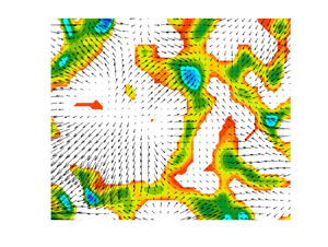
Figure 4. (a) Negative dominant eigenvalues  $\lambda _D$ of the 2D strain rate tensor $S$ (3.18), overlaid with the corresponding eigenvectors for $(Ra,Pr)=(3.33\times 10^6, 5.21)$; (b) corresponding distribution of the dimensionless horizontal divergence field, overlaid with the horizontal velocity vector field in a horizontal plane at a height of 1.5 mm from the hot plate. Panels (c,d) are the same as (a,b), but for $(Ra, Pr)= (1.21\times 10^9, 5.09)$. An arrow length of 1 mm is equal to the magnitude of horizontal velocity of 0.67 mm s $^{-1}$ in (b) while that in (d) is equal to 3.33 mm s $^{-1}$. All the plots in this figure are based on 2D3C PIV measurements. See Movies 2, 3 and 4 (see supplementary movies) showing different motions of plumes at three different $Ra$.
$Ra$.
In figure 4(a), the domain splits into slender, line-like regions that have negative  $\lambda _D$, surrounded by regions of positive $\lambda _D$. Note that the eigenvectors corresponding to $\lambda _D$ within the negative $\lambda _D$ regions in figure 4(a) are mostly perpendicular to the longitudinal boundaries of these regions. Owing to the orthogonality between the eigenvectors of $S$, the eigenvectors corresponding to the non-dominant eigenvalues within the negative $\lambda _D$ regions mostly align along the length of these regions (not shown here). The negative $\zeta$ regions in figure 4(b) have velocity vectors pointed towards them, as would be expected for plumes, since feeding of plumes by the boundary layers on their sides is predominant in the absence of strong large-scale flows at low $Ra$ (Gunasegarane & Puthenveettil Reference Gunasegarane and Puthenveettil2014).
A distribution of negative  $\lambda _D$ in slender, line-like regions is also observed in figure 4(c) at a higher Rayleigh number of $Ra=1.2\times 10^9$. Figures 4(a) and 4(c) show that an increase in $Ra$ decreases the mean spacing between the negative $\lambda _D$ regions, as expected for line plumes from (3.26) and (3.27). On comparing with the velocity vector field shown in figure 4(d), the line-like regions in figure 4(c) could be seen to be more aligned with the shear near the hot plate, compared with that in figure 4(a). Further, the orientation of the eigenvectors corresponding to $\lambda _D$, shown in figure 4(c), is seen to be more tilted along the shear direction; in contrast, for lower $Ra$, the eigenvectors are more perpendicular to the length of the $\lambda _D<0$ regions in figure 4(a). A corresponding tilt of the eigenvectors of the non-dominant eigenvalue away from the longitudinal orientation of the $\lambda _D<0$ regions thus occurs at the higher $Ra$ (not shown here).
In summary, the regions of negative  $\lambda _D$ at the smaller $Ra$ of $3.33\times 10^6$ have incoming flows with fluid elements that predominantly get compressed in directions perpendicular to the length of these regions. Such a flow and deformation is expected in a rising plume when the fluid elements get stretched vertically, resulting in dominant compression perpendicular to these plumes in a horizontal plane. These negative $\lambda _D$ regions tend to align along the dominant shear direction at higher $Ra$; plumes are known to align along the direction of large-scale flow (Puthenveettil & Arakeri Reference Puthenveettil and Arakeri2005; Shevkar et al. Reference Shevkar, Gunasegarane, Mohanan and Puthenveettil2019). At higher $Ra$, the mean spacing between these regions is smaller, resulting in the length of these regions being larger, similar to the trend observed for the length of plume regions. In the presence of shear at higher $Ra$, the compressive deformation inside these regions occurs more in the direction of shear. Such an effect would occur at larger $Ra$ since the external large-scale flow would result in a velocity field within the plume which is inclined to the longitudinal axes of the plumes (Shevkar et al. Reference Shevkar, Gunasegarane, Mohanan and Puthenveettil2019). We hence expect these regions of negative $\lambda _D$ (or negative $\zeta$) to be the plumes, while the regions with positive $\lambda _D$ (or positive $\zeta$) to be the boundary layers. Such an understanding of plume regions also imply that the boundaries of plume regions would occur at $|\lambda _1/\lambda _2|=1$, where both the extensional and the compressional strains are equal in magnitude. We now look at the connection between these regions of negative dominant eigenvalues (plumes) and LCS.
3.3. LCS and plumes
Lagrangian coherent structures is a dynamical systems-based framework to identify underlying robust features that organise tracer patterns resulting from finite time stirring in any fluid flow (Haller Reference Haller2015). While the relevance of stable and unstable manifolds for long-term advective stirring has long been known in steady, periodic and quasiperiodic flows (Beigie, Leonard & Wiggins Reference Beigie, Leonard and Wiggins1994), rigorous definitions have emerged for equivalent features that are relevant for finite-time stirring in flows of arbitrary time dependence also (Haller & Yuan Reference Haller and Yuan2000). Numerical detection of these LCS has often invoked the finite-time Lyapunov exponent (FTLE), defined as (Haller Reference Haller2002; Shadden, Lekien & Marsden Reference Shadden, Lekien and Marsden2005)
 \begin{equation} \sigma_{t_0}^{t_i}(\boldsymbol{x})=\frac{1}{|t_i|}\ln \sqrt{\lambda_{m}}, \end{equation}
where  $\lambda _{m}$ is the maximum eigenvalue of the Cauchy–Green strain tensor,
 \begin{equation} \Delta=({\boldsymbol{\nabla}} \phi_{t_0}^{t_0+t_i}(\boldsymbol{x}))^{\rm T} {\boldsymbol{\nabla}} \phi_{t_0}^{t_0+t_i}(\boldsymbol{x}), \end{equation}
with the flow map  $\phi _{t_0}^{t_0+t_i}$: $\boldsymbol {x}(t_0)\longmapsto \boldsymbol {x}(t_0+t_i)$ calculated from the advected positions of tracers from $t_0$ to $t_0+t_i$, where $t_i$ is the finite time interval of integration and superscript ${\rm T}$ indicates the transpose. Physically, FTLE is a measure of the maximum separation, after a time $t_i$, between the advected positions of infinitesimally close initial conditions around $\boldsymbol {x}$ at $t_0$. The direction associated with the maximally separating (over time $t_i$) initial conditions at $t_0$ is given by $\boldsymbol {\xi _m}$, the eigenvector corresponding to the eigenvalue $\lambda _m$.
Ridges of the backward ( $t_i<0$) and forward ( $t_i>0$) time FTLE fields have previously been computed as candidates to represent attracting and repelling LCS (together referred to as hyperbolic LCS), respectively, including in 2D (Mathur et al. Reference Mathur, Haller, Peacock, Ruppert, Jori and Swinney2007) and 3D (Green, Rowley & Haller Reference Green, Rowley and Haller2007) turbulent flows. However, since the maximum separation of initial conditions is not necessarily normal to the FTLE ridges, all FTLE ridges may not represent hyperbolic LCS (Haller Reference Haller2002). More recent approaches have identified hyperbolic LCS as maximally attracting or repelling strain lines, which, by definition, are normal to the direction $\boldsymbol {\xi _m}$ along which maximal separation of initial conditions occurs (Farazmand & Haller Reference Farazmand and Haller2012b). Attracting LCS, by definition, represent distinguished material lines along which fluid blobs get stretched. Patterns in dye release experiments therefore tend to resemble attracting LCS (Shadden, Dabiri & Marsden Reference Shadden, Dabiri and Marsden2006; Jimreeves et al. Reference Jimreeves, Mathur, Govardhan and Arakeri2018). In the turbulent ocean, even diffusive tracers such as the temperature have been shown to spatially organise, on sufficiently large scales, around the attracting LCS computed using optimally chosen integration times (Balasuriya, Ouellette & Rypina Reference Balasuriya, Ouellette and Rypina2018; Mathur et al. Reference Mathur, Jimreeves, Sharma and Agarwal2019). In RBC, Bandaru et al. (Reference Bandaru, Kolchinskaya, Padberg-Gehle and Schumacher2015) reported that, on the hot plate, thermal plumes seem to form along with attracting LCS in the skin friction field.
The choice of integration time  $t_i$ for a given flow depends on the time scales over which one is interested in understanding advective stirring and the resulting tracer patterns. In addition, constraints from the flow field dataset also impose restrictions on the value of $t_i$. For example, (i) the velocity field (from experiments or simulations) of an unsteady flow may be available only for a finite period of time, or (ii) the velocity field may be available only over a finite spatial extent, in which case numerically advected tracer particles would leave the domain of measurements in finite time. In the current study, the velocity field measurements are in a horizontal plane, and tracer particles tend to leave this plane in a few $\Delta t$, where $\Delta t\sim 0.1$ s is the temporal resolution of our measurements (see table 1). We therefore seek LCS in the limit of $t_i\to 0$, i.e. the instantaneous limit of LCS. Physically, this limit would reveal structures that drive tracer patterns in short time scales (Mattia & Haller Reference Mattia and Haller2016).
Thermal plumes entrain fluid from their longitudinal edges, thus motivating us to define plumes as hyperbolic attracting LCS. To elucidate the attracting nature of plumes even at short time scales, the horizontal deformation of a fluid parcel in the vicinity of a plume, as evidenced in a direct numerical simulation at  $(Ra, Pr)=(2\times 10^8, 1)$, captured using the Lagrangian particle tracking code of Sharma & Sameen (Reference Sharma and Sameen2019), is shown in figure 5. The fluid parcel, initiated close to the edge of a plume, is instantly pulled into the plume region and is also observed to get stretched in a way so as to align with the plume orientation in the horizontal plane. In summary, in a horizontal plane, plumes are sought as instantaneous limits of attracting LCS, and we proceed to show that regions of negative horizontal divergence are equivalent to regions in the vicinity of sufficiently strong attracting LCS in the instantaneous limit.

Figure 5. Evolution of a fluid parcel in the vicinity of a plume, as evidenced in a numerical simulation, captured using the Lagrangian particle tracking code of Sharma & Sameen (Reference Sharma and Sameen2019), at ( $Ra, Pr) = (2\times 10^8,1$). (a) Fluid particles located outside a plume at the initial time ${t^*}=0$, and (b) the advected fluid particle locations at a later time of ${t^*}=0.6$. In both (a,b), the background colour indicates the temperature distribution, with the red region being the plume central region.
For sufficiently small integration times  $t_i$, considering the 2D motion within a horizontal plane, the Cauchy–Green strain tensor (3.29) can be written as $\Delta = I + 2t_iS$, where $I$ is the $2\times 2$ identity matrix and $S$ (3.18) is the Eulerian rate of strain tensor (Nolan et al. Reference Nolan, Mattia and Shane2020). As a consequence, the forward and backward time FTLE fields (3.28) are given by
 \begin{equation} \lim_{t_i\to 0_+}\sigma_{t_0}^{t_i}=\lambda_{1},\quad \lim_{t_i\to 0_-}\sigma_{t_0}^{t_i}={-}\lambda_{2}, \end{equation}
where  $\lambda _1$ and $\lambda _2$ are the eigenvalues of $S$, as given in (3.19)–(3.20). Therefore, ridges in the $-\lambda _2$ field are candidates to represent attracting LCS in the instantaneous limit. Furthermore, the eigenvectors corresponding to the forward and backward time FTLE are the same as the eigenvectors of $S$ corresponding to $\lambda _1$ and $\lambda _2$, respectively.
Seeking regions of negative  $\lambda _2$ as regions containing ridges in the $-\lambda _2$ field, we investigate the spatial distribution of $-\lambda _2$ in figure 6. Figure 6(a) shows the spatial distribution of $-\lambda _2$ estimated from the experimental measurements at $(Ra,Pr) = (3.33\times 10^6,5.21)$, the same case as in figure 4(a). Superimposed on the $-\lambda _2$ field are the corresponding eigenvectors $\boldsymbol {\xi _2}$, which seem to be orthogonal to the ridges in most of the domain. This orthogonality indicates that ridges of the $-\lambda _2$ field are strain lines, and being local maximisers of the normal attraction rate (ridges are locally maximising features of the scalar field), they represent robust attracting LCS. When attracting LCS occur in the vicinity of repelling LCS, fluid parcels experience a combination of attracting and repelling behaviour, much like in the vicinity of saddle-type fixed points. Despite the presence of attracting LCS, repelling behaviour may dominate depending on the strength of the repelling LCS in the neighbourhood. Hence, to identify only the attraction-dominated regions as plume-like, we eliminate regions where $\lambda _1/(-\lambda _2)$ is larger than unity from the regions identified using $\lambda _2<0$, as shown later in figure 7(a). It is worth recalling from (3.30a,b) that $\lambda _1$ represents the forward time FTLE, and is hence a measure of the repelling behaviour in the region. As shown in figure 6(b), some regions of large and positive $\lambda _1$ indeed overlap with regions of positive $-\lambda _2$. For example, the region at around ( $-15$, 25) mm where $\lambda _1$ is large and positive in figure 6(b) is not plume-like even though $-\lambda _2$ is also positive there. Moreover, the positive $\lambda _1$ region around ( $-15$, 25) mm in figure 6(b) has the corresponding eigenvectors being orthogonal to the ridges in the $\lambda _1$ field, indicating the occurrence of strong repelling LCS in the region. Figure 7, as discussed later in this subsection, indeed confirms the occurrence of repelling LCS in this region.

Figure 6. (a) Spatial distribution of  $-\lambda _2$, overlaid with the corresponding eigenvectors $\boldsymbol {\xi _2}$ for ( $Ra$,
$Ra$,  $Pr$) = (3.33 $\times 10^6$, 5.21); (b) corresponding distribution of $\lambda _1$, overlaid with the corresponding eigenvectors $\boldsymbol {\xi _1}$ in a horizontal plane at a height of 1.5 mm from the hot plate. Panels (c,d) are the same as (a,b), but for ( $Ra$,
$Ra$,  $Pr$) = ( $1.21\times 10^9$, 5.09). All the plots in this figure are based on experimental 2D3C PIV measurements.

Figure 7. Attracting and repelling LCS in the instantaneous limit (integration time  $t_i=0$) based on 2D3C velocity measurements in the experiment at ( $Ra, Pr)=(3.33\times 10^6,5.21)$. (a) Attracting LCS (blue lines) overlaid over $\lambda _D$ field (regions of positive $\lambda _D$ are shown in white), (b) attracting (blue) and repelling (red) LCS plotted together.
In summary, in figure 6(a,b), regions of negative  $\lambda _2$, with $-\lambda _2/\lambda _1<0$ or $-\lambda _2/\lambda _1>1$, indicate regions of attracting LCS with no repelling LCS that are stronger, and are hence plume-like. Based on the various scenarios shown in table 2, plumes can now be identified as regions where $\lambda _2$ is dominant and negative, which coincide with regions of $\boldsymbol {\nabla _H}\boldsymbol {\cdot }\boldsymbol {u}<0$. It is insightful to recall from the study of Mensa et al. (Reference Mensa, Özgökmen, Poje and Imberger2015) that horizontal divergence and tracer concentration fields were found to be highly correlated in a model ocean mixed layer with weak wind forcing. Our analysis provides a complementary perspective that the horizontal divergence field is highly correlated with regions of sufficiently strong attracting LCS. Attracting LCS, by their very definition, significantly influence tracer concentration fields, thus establishing that our discussion is consistent with the conclusions of Mensa et al. (Reference Mensa, Özgökmen, Poje and Imberger2015).
In figure 6(c,d), we reproduce figures 6(a) and 6(b) for a larger  $Ra$ of $1.21\times 10^9$, which corresponds to a larger shear imposed on the regions close to the hot plate due to a stronger large-scale flow at the higher $Ra$. Regions of positive $-\lambda _2$ extract plume-like regions (figure 6c), but with the corresponding eigenvectors being somewhat non-orthogonal to the ridges of the $-\lambda _2$ field. We attribute this non-orthogonality to the presence of shear, which in some extreme scenarios can even introduce non-hyperbolic FTLE ridges (Haller Reference Haller2002). Regions inside the plumes, however, are known to have relatively low shear (Shevkar et al. Reference Shevkar, Gunasegarane, Mohanan and Puthenveettil2019; Blass et al. Reference Blass, Zhu, Verzicco, Lohse and Stevens2020), owing to which ridges in the $-\lambda _2$ field are likely to represent attracting LCS even at high $Ra$. In summary, attracting LCS in regions where repelling LCS are either absent or sufficiently weak are interpreted as the centrelines of plume regions. Finally, the $\lambda _1$ field in the regions of positive $-\lambda _2$ shown in figure 6(d) show that stronger repelling LCS can occur in the regions of attracting LCS, with such regions not considered plume-like.
We now extract variational theory-based attracting and repelling LCS (Farazmand & Haller Reference Farazmand and Haller2012a), based on the instantaneous limits of forward-time and backward-time FTLEs ( $\lambda _1$ and $-\lambda _2$, respectively) and the corresponding eigenvectors, using the MATLAB-based software discussed in Onu, Huhn & Haller (Reference Onu, Huhn and Haller2015). Specifically, attracting LCS are obtained as trajectories of the differential equation
 \begin{equation} \frac{{\rm d}\boldsymbol{r}}{{\rm d}t}={\pm} \boldsymbol{\xi_1}(\boldsymbol{r}), \end{equation}
where  $\boldsymbol {r}=(x,y)$ is the position vector and $\xi _1$ is the eigenvector corresponding to $\lambda _1$. These trajectories are initialised from local maxima of $-\lambda _2$, that lie in $\lambda _D<0$ regions, and are stopped based on the specification of a maximum length. Correspondingly, repelling LCS are obtained as trajectories of ${{\rm d}\boldsymbol {r}}/{{\rm d}t}=\pm \boldsymbol {\xi _2}(\boldsymbol {r})$, with initialisation points being from local maxima of $\lambda _1$ that lie in $\lambda _D>0$ regions. More details can be found in Onu et al. (Reference Onu, Huhn and Haller2015).
For the experimental measurements corresponding to figure 6(a), figure 7(a) shows the attracting LCS plotted on top of the  $\lambda _D$ field, for which only the negative valued regions are shown in colour. While all the $\lambda _D<0$ regions have attracting LCS passing through them, attracting LCS also pass through regions where $\lambda _D>0$. Noticeable examples of such regions are marked as A, B, C, D, E and F in figure 7(a). Figure 7(b) shows that these regions have corresponding repelling LCS passing in their vicinity, with the repelling behaviour being dominant since $\lambda _D = \lambda _1>0$. It is also noteworthy that regions of intersection between attracting and repelling LCS are saddle-like and hence less likely to be plume regions.
Finally, to highlight the ability of  $\boldsymbol {\nabla _H}\boldsymbol {\cdot }\boldsymbol {u}$ to pick up regions of negative $\lambda _D$, we plot the correlation between $\boldsymbol {\nabla _H}\boldsymbol {\cdot }\boldsymbol {u}$ and $\lambda _D$ from the entire spatial domain, averaged over 1399 snapshots, as a function of $Ra$ in figure 8. Values close to unity indicate that $\boldsymbol {\nabla _H}\boldsymbol {\cdot }\boldsymbol {u}$ can be a reliable indicator of regions with negative $\lambda _D$. Furthermore, the similarly large correlation between $\boldsymbol {\nabla _H}\boldsymbol {\cdot }\boldsymbol {u}$ and $\lambda _2$ suggests that regions with negative $\lambda _2$ and positive dominant $\lambda _1$ represent a relatively small fraction of the spatial domain at all $Ra$.
$Ra$.

Figure 8. The temporal mean values of the correlation coefficient between ◆ (blue),  $\boldsymbol {\nabla }_H \boldsymbol {\cdot } \boldsymbol {u}$ values and the dominant eigenvalues and ■ (red), $\boldsymbol {\nabla }_H\boldsymbol {\cdot }\boldsymbol {u}$ and $\lambda _2$ values for the present range of $Ra$ in experiments. The correlation coefficient between arrays $P$ and $Q$ is defined as $r=\sum _{m} \sum _n (P_{mn}-\langle P\rangle _A)(Q_{mn}-\langle Q\rangle _A)/\sqrt {(\sum _{m} \sum _n (P_{mn}-\langle P\rangle _A)^2)(\sum _{m} \sum _n (Q_{mn}-\langle Q\rangle _A)^2)}$, where $\langle P\rangle _A$ and $\langle Q\rangle _A$ indicate spatial means.
3.4. Spatial distribution of eigenvalues
Based on (3.19)–(3.21), we define the dimensionless second eigenvalue as
 \begin{equation} \kappa=2\lambda_2/\gamma, \end{equation}
representing twice the ratio of the corresponding extensional or compressional strain rate – as the case may be based on whether  $\lambda _2$ is positive or negative – with the total strain rate. Instantaneous snapshots of the spatial distribution of $\kappa$ are shown in figures 9(a) and 9(b) for $Ra=3.33\times 10^6$ and $Ra=1.2\times 10^9$, respectively. Regions with positive $\lambda _1$ and $\lambda _2$ (case 1 in table 2) are the boundary layer regions where strong local impingement occurs, and the fluid elements get stretched in both the horizontal principal directions; such regions are shown in maroon in figure 9. Regions with positive $\lambda _1$ and negative $\lambda _2$ with $\lambda _1$ being dominant (case 2 in table 2) are the boundary layer regions with little or no impingement, where the extensional strain dominates over the compressional strain; such regions are shown in red in figure 9. In the plume regions where the compressional strain dominates over the extensional strain, $\lambda _1$ is positive and $\lambda _2$ is negative with $\lambda _2$ being dominant (case 3 in table 2); such regions are shown in green/yellow in figure 9. Regions with negative $\lambda _1$ and $\lambda _2$ (case 4 in table 2) seem to occur at the centre of the plumes, such regions are shown in blue/cyan in figure 9. At low $Ra$ (figure 9a), a converging (in all directions) type of flow is observed in these regions, possibly due to the larger vertical velocity at the centre of the plumes; fluid elements would then get compressed in all directions in the horizontal plane due to the large vertical stretching by the rising plume. At higher $Ra$ (figure 9b) these plume centre regions with a converging flow are smaller in extent, possibly due to the stronger effect of shear from the large-scale flow. In table 2, cases 1 and 4 correspond to impingement portions of the boundary layer and central plume regions, respectively. Regions in the vicinity of boundary layer – plume boundaries are more faithfully captured by cases 2 and 3; case 2 being on the boundary layer side and case 3 being on the plume side.

Figure 9. Spatial distribution of the dimensionless  $\lambda _2$ (3.32), with the corresponding horizontal velocity vector field overlaid at (a) $Ra=3.33\times 10^6$ and (b) $Ra=1.21\times 10^9$.
The shear fields created due to LSF can be seen from the directions and magnitudes of horizontal velocity vectors in figures 9(a) and 9(b), as well as in figures 4(b) and 4(d), at  $Ra=3.33\times 10^6$ and $Ra=1.21\times 10^9$, respectively. The scales of vector lengths are given in the caption of figure 4. In RBC, inside a box, large-scale flow is known to get oriented along one of the diagonals of a box and may change its orientation along the other diagonal with time. At lower $Ra$, due to the elliptic shape of LSF path (Niemela & Sreenivasan Reference Niemela and Sreenivasan2003), only a small near-plate area comes in direct contact with the LSF. As seen in figure 9(a), at lower $Ra$, the vectors are of smaller magnitudes and are randomly oriented, and so are the plumes; implying that the effect of shear due to the LSF on the near-plate region is minimal. Increase in $Ra$ increases the large-scale flow strength (3.25). Also, with increasing $Ra$, the shape of the LSF path gets changed from elliptic to increasingly square-like (Niemela & Sreenivasan Reference Niemela and Sreenivasan2003), which in-effect causes larger and larger near-wall areas to get affected by the LSF. At high $Ra$, due to this increased LSF strength, and the square-like nature of the LSF path along the diagonal of the box, a unidirectional shear field, with plumes oriented in the direction of shear, is created in the centre of a horizontal plane close to the hot plate (Shevkar et al. Reference Shevkar, Gunasegarane, Mohanan and Puthenveettil2019), as shown in figure 9(b). At any $Ra$, the effect of LSF is felt the most at the central region of the bottom plate, and the effect decreases as we move away from the centre towards the sidewalls.
For various eigenvalue combinations, we now categorise the flow field into four different regions based on the value of  $\kappa$. It is evident from (3.20) that $\kappa =-1$ is satisfied when $\boldsymbol {\nabla _H}\boldsymbol {\cdot }\boldsymbol {u}=0$. As a result, regions with $\kappa \geq -1$ correspond to boundary layer regions, while regions with $\kappa <-1$ correspond to plume regions. As discussed earlier in the section, cases 1 and 2, separated by the $\lambda _2 = 0$ boundary, further divide the boundary layer regions into impingement ( $\lambda _1>\lambda _2>0$) and non-impingement ( $\lambda _1>0>\lambda _2$ with $\lambda _1$ being dominant) portions. In terms of $\kappa$, impingement and non-impingement portions of the boundary layer regions are given by $\kappa >0$ and $-1<\kappa <0$, respectively. Similarly, the plume regions given by $\kappa <-1$ are divided further as convergent-in-all-directions ( $\lambda _2<\lambda _1<0$) and remaining ( $\lambda _2<0<\lambda _1$ with $\lambda _2$ being dominant) portions. In terms of $\kappa$, $\kappa <-2$ and $-2<\kappa <-1$ correspond to convergent-in-all-directions plume and remaining plume regions, respectively.
The aforementioned classification based on the values of  $\kappa$ is shown using different colours in figure 9. While the impingement and non-impingement boundary layer regions are shown in maroon and red, respectively, the convergent-in-all-directions and remaining plume regions are shown in blue/cyan and green/yellow, respectively. Based on similar arguments, it is also possible to perform the classification based on the values of non-dimensionalised $\lambda _1$, given by $\chi = 2\lambda _1/\gamma$. Specifically, the boundary layer regions correspond to $\chi >2$ (impingement) and $1<\chi <2$ (non-impingement), while the plume regions correspond to $\chi <0$ (convergent-in-all-directions) and $0<\chi <1$ (remaining plume regions).
In summary, the plume regions have  $\boldsymbol {\nabla _H} \boldsymbol {\cdot } \boldsymbol {u}<0$, which can be alternatively expressed as $\kappa <-1$ or $\chi <1$. Since these regions have $\lambda _D=\lambda _2$, which is negative, these regions have the dominant compression more than half the total strain, i.e. $|\lambda _2|>\gamma /2$. Within such plume regions, case 3 regions tend to occur on the edges of the plumes where shear strain, and hence the total strain, could be significant so that the dominant compressional strain $\lambda _2$ in these regions is in the range $\gamma /2<\lambda _2<\gamma$. These are the regions of the plumes that are affected by the shear due to the large-scale flow; we expect the extent of these regions to increase with $Ra$. At the convergent-in-all-directions portions of the plumes, where shear effects are not significant, we find case 4 regions where the dominant compressive strain $\lambda _2>\gamma$, the total strain.
The boundary layer regions have  $\boldsymbol {\nabla _H} \boldsymbol {\cdot } \boldsymbol {u}>0$, alternately expressed as $\chi >1$ or $\kappa >-1$. These regions have $\lambda _D=\lambda _1$, which is positive. Then, these regions have dominant extensional strain more than half the total strain, $\lambda _1>\gamma /2$. These boundary layer regions have within them case 1 regions, which occur in the impingement regions, and have dominant extensional strain $\lambda _1$ more than the total strain $\gamma$. These regions are surrounded by case 2 regions, which occur at the edge of these boundary layer regions, and have non-negligible shear strain, and hence total strain $\gamma$, so that the dominant extensional strain satisfies $\gamma >\lambda _1>\gamma /2$. These are the regions of the boundary layers that are affected by the external shear. Hence, it appears that the effects of external shear due to the large-scale flow are more strongly felt at the edges of the boundary layers and plumes, with the beginning of the boundary layer regions and the centre of plumes being relatively less affected by the large-scale flow.
The present criterion for detecting plumes,  $\boldsymbol {\nabla _H} \boldsymbol {\cdot } \boldsymbol {u}<0$, which we showed to be equivalent to $\lambda _D<0$ in § 3.2 and equivalent to $\kappa =2\lambda _2/\gamma <-1$ in this subsection, picks up the plume regions along with their edges. In addition, the central plume regions are detected by local minima of $-\lambda _2$ or $\kappa$, where shear effects are minimal. Similarly, attracting LCS in the instantaneous limit occur in regions where shear is not dominant, and can hence be expected to pass through the middle of the $\boldsymbol {\nabla _H}\boldsymbol {\cdot }\boldsymbol {u}<0$ regions. While $\boldsymbol {\nabla _H}\boldsymbol {\cdot }\boldsymbol {u}=0$ identifies the plume boundaries, and hence allows us to estimate the widths of the plume structures, the LCS perspective only allows for us to extract lines that pass through the centre of the plume regions. Additional criteria are required for the LCS-based approach to detect the plume boundaries.
4. Verification of the  ${\nabla _H} {\cdot } {u}$ criterion

As we have already seen in §§ 3.2, 3.3 and 3.4, qualitative considerations strongly suggest that the  $\boldsymbol {\nabla }_H\boldsymbol {\cdot }\boldsymbol {u}<0$ regions are the line plumes. In § 4.1, we now quantitatively verify whether the overall lengths and areas of $\boldsymbol {\nabla }_H\boldsymbol {\cdot }\boldsymbol {u}<0$ regions match the corresponding theoretical predictions for plumes. In § 4.2, we compare the $\boldsymbol {\nabla }_H\boldsymbol {\cdot }\boldsymbol {u}<0$ criterion with the other existing plume detection criteria.
4.1. Verification with the theoretical estimate of length and area of plumes
The length of plumes in an area  $A$, as given by Puthenveettil et al. (Reference Puthenveettil, Gunasegarane, Agrawal, Schmeling, Bosbach and Arakeri2011), is
 \begin{equation} L_p=A/\bar{\lambda}, \end{equation}
where  $\bar {\lambda }$ is given by (3.26). Substituting (3.26) in (4.1), we obtain
 \begin{equation} L_p=\frac{1}{2^{1/3}C_1Pr^{n_1}}\frac{A}{H}Ra^{1/3}, \end{equation}
thus giving  $L_p$ as a function of $Ra$ and $Pr$ (Puthenveettil et al. Reference Puthenveettil, Gunasegarane, Agrawal, Schmeling, Bosbach and Arakeri2011). Equation (4.2) has been verified with measurements of plume lengths – obtained by representing the plume regions in areas $A$ with short linear segments – over six decades of $Ra$, three decades of $Pr$ and a wide range of $A$ by Puthenveettil et al. (Reference Puthenveettil, Gunasegarane, Agrawal, Schmeling, Bosbach and Arakeri2011), using planforms from experimental and numerical studies. We now compare the total length of negative $\boldsymbol {\nabla }_H\boldsymbol {\cdot }\boldsymbol {u}$ regions in an area $A$ with equation (4.2) to quantitatively verify whether the negative $\boldsymbol {\nabla }_H\boldsymbol {\cdot }\boldsymbol {u}$ regions are plumes. The total length of the negative $\boldsymbol {\nabla }_H\boldsymbol {\cdot }\boldsymbol {u}$ regions in various areas $A$, from our experimental and computational velocity fields, were measured by representing these regions with short linear segments, as done in Puthenveettil et al. (Reference Puthenveettil, Gunasegarane, Agrawal, Schmeling, Bosbach and Arakeri2011). The sum of the length of these segments gives the total length of the negative $\boldsymbol {\nabla }_H\boldsymbol {\cdot }\boldsymbol {u}$ regions. Figure 10(a) shows the measured total length of the negative $\boldsymbol {\nabla }_H\boldsymbol {\cdot }\boldsymbol {u}$ regions, along with (4.2) for the range of $Ra$ and $Pr$ considered in the present study. The error bars show the range of data from measurements at different instants at the same $Ra$. The excellent agreement between (4.2) and the measured lengths of negative $\boldsymbol {\nabla }_H\boldsymbol {\cdot }\boldsymbol {u}$ regions indicates that these regions are indeed the plumes.

Figure 10. (a) Variation of the measured total length of the negative  $\boldsymbol {\nabla }_H\boldsymbol {\cdot }\boldsymbol {u}$ regions with $Ra$. The error bars show the ranges of values obtained from 10 different instants. Here $\blacktriangle$ (red) are experiments at the $Ra$ and $Pr$ shown in table 1. Computations at $Ra=2\times 10^7$ and $2\times 10^8$ for $\circ$ (blue), $Pr=1$; $\diamond$ (magenta), $Pr=10$; $\square$ (green), $Pr=4.96$; and $--$ (4.2). (b) Variation of the measured area fraction of the $\boldsymbol {\nabla }_H\boldsymbol {\cdot }\boldsymbol {u}<0$ regions with $Ra$ with $n=0.09$. The error bars show one standard deviation of measurements from various instants. Symbols denote the same quantities as in (a), $--$ (4.9).
We now obtain a theoretical estimate of the area fraction  $A_p/A$ of the plumes, where $A_p$ is the area of the plumes in an area $A$, so as to compare the measured values of the area fractions of the $\boldsymbol {\nabla }_H\boldsymbol {\cdot }\boldsymbol {u}<0$ regions with this theoretical estimate; this serves as another verification of the $\boldsymbol {\nabla }_H\boldsymbol {\cdot }\boldsymbol {u}<0$ criterion. Plumes are a result of instability of the natural convection boundary layers on either side of the plumes. Due to this, the mean thickness of the plumes in a horizontal plane ( $t_{pc}$) at the height the boundary layers turn into plumes is known to scale as the boundary layer thickness (Van der Poel et al. Reference Van der Poel, Verzicco, Grossmann and Lohse2015). Then,
 \begin{equation} t_{pc}\sim 2 \delta_{vc}, \end{equation}
twice the critical velocity boundary layer thickness,  $\delta _{vc}$. For any $Pr$, the total area of the plumes in an area $A$ is then
 \begin{equation} A_p\sim t_{pc} L_p, \end{equation}
where  $L_p$ is given by (4.2). From (4.3) and (4.4),
 \begin{equation} \frac{A_p}{A} =C(Pr)2\delta_{vc}\frac{L_p}{A}, \end{equation}
where  $C(Pr)$ is an unknown function of $Pr$ to take into account the effects of $Pr$ on the instability of the boundary layers. Using the expressions for the critical thermal boundary layer thickness $\delta _c\sim 4\bar {\lambda }/(Gr_\lambda Pr)^{1/5}$ and the ratio $\delta _c/\delta _{vc}\sim 1/\sqrt {Pr}$, given as (A11) and (A17), respectively, in Puthenveettil et al. (Reference Puthenveettil, Gunasegarane, Agrawal, Schmeling, Bosbach and Arakeri2011),
 \begin{equation} \delta_{vc}\sim \frac{4\bar{\lambda} Pr^{2/5}}{Gr_\lambda^{1/5}}. \end{equation}
Here,  $Gr_\lambda =g\beta \Delta T_w \overline {\lambda }^3/\nu ^2$ is the Grashoff number based on the mean plume spacing $\bar {\lambda }$. Substituting (3.26) for $\bar {\lambda }$ into (4.6), we obtain
 \begin{equation} \delta_{vc}\sim \left(\frac{C_1}{2}\right)^{2/5}Pr^{0.54}Z_w, \end{equation}
where  $Z_w$ is the near wall length scale given by (3.27). Substituting (4.7) and (4.2) in (4.5), we obtain the theoretical estimate of the area fraction of plumes as
 \begin{equation} \frac{A_p}{A}=0.15\,C(Pr)\,Pr^{0.44}. \end{equation}
Interestingly, (4.8) – an important new result of the present work – shows that the area fraction of plumes near the hot surface in turbulent RBC is independent of  $Ra$, and is only a function of $Pr$. Even though the total length of plumes ( $L_p$) increases as $Ra^{1/3}$ by (4.2), their corresponding mean thickness ( $2\delta _{vc}$) decreases as $Ra^{-1/3}$ (see (4.7) and (3.27)) so that the area fraction of plumes $A_p/A$ becomes independent of $Ra$.
$Ra$.
Figure 10(b) shows the measured areas of the  $\boldsymbol {\nabla }_H\boldsymbol {\cdot }\boldsymbol {u}<0$ regions, normalised by the total area, from the experimental and the computational velocity fields for $1\le Pr\le 10$ and $5\times 10^5\le Ra \le 1 \times 10^9$. The measured area fractions shown in the figure are averaged from those obtained at various instants at a given ( $Ra$,
$Ra$,  $Pr$), with the error bars showing one standard deviation range of these instantaneous values. The measured mean area fractions of the $\boldsymbol {\nabla }_H\boldsymbol {\cdot }\boldsymbol {u}<0$ regions collapse on to the relation
 \begin{equation} \frac{A_p}{A}= 0.55\,Pr^{{-}0.09}, \end{equation}
shown by the dashed line in the figure. The measured mean area fractions are also independent of  $Ra$, in agreement with the theoretical relation (4.8), thereby validating the $\boldsymbol {\nabla }_H\boldsymbol {\cdot }\boldsymbol {u}<0$ criterion. Comparison of (4.9) with (4.8) implies that $C(Pr)=3.67Pr^{-0.53}$ captures the $Pr$ effects on the instability of the boundary layer.
4.2. Comparison with other criteria for detecting plumes
In this subsection, we compare the plumes extracted by the  ${\nabla ^{*}}_H\boldsymbol {\cdot }\boldsymbol {u^{*}}<0$ criterion, when applied to the velocity fields obtained from our numerical computations, with those extracted by the criterion in (1.1) (Gastine et al. Reference Gastine, Wicht and Aurnou2015) and the criterion
 \begin{equation} w^*T^{*'} > 0, w^{*}>0. \end{equation}
Here, in addition to  $w^{*}T^{*'}>0$ mentioned by Schumacher (Reference Schumacher2009), we include $w^{*}>0$ since we are only interested in rising plumes close to the bottom plate. The criterion (1.1), which we use with $c=0.25$, is a temperature based criterion while the criterion (4.10) is a flux-based criterion. The plumes extracted by the three criteria (3.17), (1.1) and (4.10) in a horizontal plane at a height within the natural convection boundary layer, are compared for $Pr=1,\, 4.98$ and $10$ at $Ra=2\times 10^7$. The plumes from these criteria are assessed vis-à-vis the dimensionless positive vertical velocity ( $w^{*}>0$) field and the dimensionless temperature field $T^*$ in the same plane. A theoretical comparison of the present $\boldsymbol {\nabla }_H\boldsymbol {\cdot }\boldsymbol {u}<0$ criterion with the $w>0$ condition using similarity solutions described in § 3.1 is given in Appendix B; a similar comparison with the flux criterion, using 2D boundary layer equations, is given in Appendix C. We also show in Appendix D that application of methods for identification of coherent structures in shear turbulence (Hunt et al. Reference Hunt, Wray and Moin1988; Jeong & Hussain Reference Jeong and Hussain1995; Zhou et al. Reference Zhou, Adrian, Balachandar and Kendall1999) fail to detect the complete plume structure.
Figure 11(c–e) show the plumes detected by the above three criteria, along with the dimensionless temperature field in figure 11(a) and the  $w^{*}>0$ regions in figure 11(b), all at $z/H=0.012$ for $Ra=2\times 10^7$ and $Pr=1$. Overall, all the three criteria detect similar regions, which have higher temperatures and $w^{*}>0$. However, the horizontal divergence criterion (3.17) detects high temperature upwellings such as the connecting plumes at D and E (see figure 11d), isolated initiation of plumes at F and upwellings in-between merging plumes at G (see figure 11e); these commonly occurring regions are all excluded by both the criteria (1.1) and (4.10). In addition, there are a few regions, such as A and B in figure 11(b) and C in figure 11(c), which have temperatures quite higher than the mean temperature, but have $w^{*}<0$. Such regions are seen to occur in-between two merging plumes. A purely temperature-based criterion, such as (1.1), erroneously identifies these regions as plumes, as seen in figure 11(d). The kinematic condition $\boldsymbol {\nabla }^{*}_H\boldsymbol {\cdot }\boldsymbol {u^{*}}<0$ excludes such regions since these are not regions where there is an upward acceleration. A flux-based criterion, such as (4.10), also excludes such regions (see figure 11e) since the flux is downward due to $w^{*}<0$ in such regions. Further, (1.1) and (4.10), in general, select narrower plume regions, missing out the upwellings which occur at the edges of upwelling regions that have higher than mean temperatures, as seen in the specific case of the plume at H in figure 11(e).

Figure 11. Plumes detected by various criteria at  $Ra=2\times 10^7$ at three $Pr$: (a–e), $Pr=1$, $z/H= 0.012$; (f–j), $Pr=4.96$, $z/H=0.029$; (k–o), $Pr=10$, $z/H=0.043$. (a,f,k) The temperature field; (b,g,l), the positive vertical velocity field; (c,h,m), $\boldsymbol {\nabla ^{*}_H} \boldsymbol {\cdot } \boldsymbol {u^{*}}<0$; (d,i,n), the criterion by Gastine et al. (Reference Gastine, Wicht and Aurnou2015) (1.1); (e,j,o), the criterion by Schumacher (Reference Schumacher2009) with $w^{*}>0$ (4.10).
In figure 12, we compare the evolution of the instantaneous area fractions of plumes ( $A_{pi}/A$) with time in a horizontal plane at $z/H=0.012$ for $(Ra, Pr)=(2\times 10^7,1)$ using the above three criteria (3.17), (1.1) and (4.10), along with the $w^{*}>0$ regions and the $T^{*}>0.75$ regions. A theoretical estimate for the corresponding time averaged area fraction of plumes ( $A_p/A$) was obtained in (4.8). In the present calculations of $A_{pi}/A$, a circular area within $r^*=0.352$ is taken as $A$ to avoid the influence of the sidewall. The overall trend of $A_{pi}/A$ with time is the same for all these criteria, even though there are differences in the magnitudes and the details at specific time instants, such as at $t^{*}=7, 28, 51$ and $61$. The area fractions estimated from $\boldsymbol {\nabla }^{*}_H\boldsymbol {\cdot }\boldsymbol {u^{*}}<0$ follow the trend of the $w^{*}>0$ regions quite closely, but is always slightly lower in magnitude. This slightly lower area of plumes estimated from (3.17), compared with that from $w^{*}>0$, can also be seen in figure 11(c,b), especially in the larger plume area at F and E in figure 11(b), compared with the corresponding regions in figure 11(c). The edges of the $w^{*}>0$ regions, which do not have buoyancy driven vertical acceleration, are, possibly correctly, not considered as plumes by the horizontal divergence criterion. Further, as shown in (B4a–d), (3.17) implies that, in addition to $w=0$, the edge of the plume must also have $\partial w/\partial z =0, \partial w/\partial x =0$ and $\partial u/\partial x=0$; these more stringent conditions seem to shift the plume boundary calculated from (3.17) slightly inward into the upwelling regions, so as to result in slightly lower plume areas compared with that with a $w>0$ condition. It must also be remembered that a $w>0$ criterion would wrongly identify all the upward flow regions in the up-flow region of the large-scale flow as plumes.

Figure 12. Time series of instantaneous plume area fractions detected by  $T^{*}\ge 0.75$ (in black), $w^{*}>0$ (in red), $\boldsymbol {\nabla ^{*}_H}\boldsymbol {\cdot } \boldsymbol {u^{*}} >0$ (in green), (1.1) (in magenta) and (4.10) (in blue) at $Ra=2\times 10^7$ and $Pr=1$. The inset shows the $T^{*}>0.75$ regions in green, yellow and red colour at $t^{*}=51$, with the $w^{*}=0$ boundary shown by the dashed line, while the regions where $T^{*}<0.75$ and $w^{*}<0$ are shown in light blue.
The criteria (1.1) and (4.10) closely follow the trend of the area evolution of the  $T^{*}\ge 0.75$ regions, albeit with noticeably smaller areas at all instants. Similarly, the areas captured by (1.1) and (4.10) are much lower than those from (3.17) and $w^{*}>0$. These three criteria, viz. $T^{*}\ge 0.75$, (1.1) and (4.10), however, show substantial deviations from the velocity based criteria, viz. (3.17) and $w^{*}>0$, at some specific time instants, such as at $t^{*}=7, 28, 51$ and $61$. The plume areas estimated by $T^{*}\ge 0.75$ at these times show a sudden rise to values approximately 40 % more than the mean area fractions; similar trends are shown by the (1.1) and the (4.10) criteria, even though their mean area fractions are lower. We examine one such instant at $t^{*}=51$ in the inset in figure 12. The inset figure shows that there are large regions where $T^{*}> 0.75$, which, however, have $w^{*}$ slightly less than zero, possibly due to reasons like the hotter rising fluid bouncing back down after hitting the top plate, or due to the stronger downward entrainment of hotter fluid in-between two nearby rising strong plumes. The spike in $A_{pi}/A$ shown by the $T^{*}\ge 0.75$ condition and by the criteria (1.1) and (4.10) are due to such regions being erroneously classified as plumes.
At a higher Prandtl number,  $Pr=4.96$, the structure is less intricate in figure 11(g) compared with that in figure 11(b), possibly due to the increase in viscous effects. Comparing figures 11(g) and 11(b), we see that the upwellings at $Pr=4.96$ are mostly of the same thickness as at $Pr=1$. The plumes, however, have thinner higher temperature regions, as could be noticed by comparing figures 11(f) and 11(a). A temperature criterion such as $T^{*}>0.75$ at this $Pr$ would then detect much smaller area of plumes, as seen in the temporal evolution of plume areas at $Pr=4.96$ in figure 13(a). The $T^{*}\ge 0.75$ criterion, which gave $A_{pi}/A\approx 0.5$ for $Pr=1$ in figure 12, now detects a much smaller area of plumes at $Pr=4.96$, with $A_{pi}/A\approx 0.1$ in figure 13(a). The fraction of areas of velocity upwellings at $Pr=4.96$, however, remains at approximately $0.45$ in figure 13(a), around the same value as at $Pr=1$ in figure 12.

Figure 13. (a) The time series of instantaneous plume area fractions at  $Ra=2\times 10^7$ and $Pr=4.96$ detected by $T^{*}\ge 0.75$ (in black), $w^{*}>0$ (in red), $\boldsymbol {\nabla ^{*}_H}\boldsymbol {\cdot } \boldsymbol {u^{*}} >0$ (in green), (1.1) (in magenta) and (4.10) (in blue). (b) Correlation coefficients between $T^{*}$ and $\boldsymbol {\nabla ^{*}_H} \boldsymbol {\cdot } \boldsymbol {u^{*}}$ (in black), $T^{*}$ and $w^{*}$ (in red) and $w^{*}$ and $\boldsymbol {\nabla ^{*}_H} \boldsymbol {\cdot } \boldsymbol {u^{*}}$ (in green). Circles denote $Ra=2\times 10^7$ and triangles denote $Ra=2\times 10^8$. The error bars are plotted using the ranges of values obtained in five instants.
Figure 11(h) shows that the criterion (3.17) captures all these upwellings at this higher  $Pr$ with their actual thicknesses. The $w^{*}>0$ areas and the $\boldsymbol {\nabla }^{*}_H\boldsymbol {\cdot }\boldsymbol {u^{*}}<0$ areas coincide at all instants at this higher $Pr$, as seen in figure 13(a). The divergence criterion, however, seems to slightly underestimate the downward flow, non-plume regions in-between large upwellings, as seen at I in figure 11(g); such regions are, however, only a small fraction of the plume area. On the contrary, the criteria (1.1) and (4.10), capture approximately $40\,\%$ fewer upwelling areas, as seen in figure 13(a); the reason being the much thinner regions characterised as plumes by these criteria at $Pr=4.96$ (see figure 11i,j vis-à-vis figure 11g). These two criteria seem to be able to capture only the thermal boundary layer regions of the plumes, which are thinner compared with the velocity boundary layers at $Pr>1$. The two criteria (1.1) and (4.10) miss large upwell regions such as an entire plume at L in figure 11(i). The two criteria also miss out upwellings on the outer peripheries of higher temperature regions, such regions such as J and K in figure 11(h).
A further increase in  $Pr$ reduces the intricacy of the plume patterns further; see the upwelling patterns shown in figure 11(l) at $Pr=10$ and those in figure 11(g,b) at $Pr=4.96$ and $Pr=1$, respectively. The thickness of the upwellings in these figures remains approximately the same, while the high temperature regions in figure 11(k) become even thinner than in figure 11(f). The $\boldsymbol {\nabla ^{*}_H}\boldsymbol {\cdot } \boldsymbol {u^{*}}<0$ criterion identifies all the upwelling regions as plumes, while the criteria (1.1) and (4.10) mostly identify only the thinner, higher temperature regions as plumes, often missing entire large upwelling regions, such as the plume at M in figure 11(l). However, the divergence criterion (3.17) seems to slightly overestimate the plume regions with downwelling regions near the edges of the upwellings, especially when they are closed polygons, such as at N and O in figure 11(m), also being identified as plumes; these are, however, quite small areas compared with the overall plume areas.
This increasing difference between the areas of upwelling regions and the areas of higher temperature regions with an increase in  $Pr$ could be seen in figure 13(b), which shows the correlation coefficient between $T^{*}$ and $\boldsymbol {\nabla ^{*}_H}\boldsymbol {\cdot } \boldsymbol {u^{*}}<0$ for various $Ra$ and $Pr$. As discussed earlier, with increase in $Pr$, the higher temperature region areas, compared with the upwelling region areas, shrink in their thickness (see figures 11f, 11g vis-à-vis figures 11a, 11b, and figures 11k, 11l vis-à-vis figures 11f, 11g). This occurs since the thermal boundary layers become thinner compared with the viscous boundary layer with increase in $Pr$. Correspondingly, the correlation between $T^{*}$ and $\boldsymbol {\nabla ^{*}_H}\boldsymbol {\cdot }\boldsymbol {u^{*}}$ in figure 13(b) decreases from around $0.85$ to $0.7$ with increase in $Pr$ from $1$ to $10$, showing that temperature-based criteria will detect increasingly smaller areas as plumes, compared with the upwelling regions, with increasing $Pr$. Due to the same reason, a decrease in correlation between $T^{*}$ and $w^{*}$ with increase in $Pr$ is also seen in figure 13(b). In contrast, the correlation between $\boldsymbol {\nabla ^{*}_H}\boldsymbol {\cdot }\boldsymbol {u^{*}}$ and $w^{*}$ is high and varies little (between $1$ and $0.95$) with $Pr$, showing the capability of the $\boldsymbol {\nabla ^{*}_H}\boldsymbol {\cdot }\boldsymbol {u^{*}}<0$ criterion to pick up the upwellings as plumes at all $Pr\ge 1$.
5. Discussion and conclusions
The primary contribution of the present work is the proposal, justification and validation of the novel kinematic criterion of negative horizontal divergence ( ${\boldsymbol {\nabla _H}\boldsymbol {\cdot }\boldsymbol {u}<0}$) to separate plumes from the local boundary layers near the hot plate in turbulent convection. We showed that this simple criterion represents an improvement over other criteria for detection of plumes, over the range of Rayleigh numbers $5.52\times 10^5\le Ra\le 1.2\times 10^9$ and Prandtl numbers $1\le Pr\le 10$. The criterion picks up all the local buoyancy-driven upwellings as plumes, which the other presently available criteria often fail to do. The proposed criterion needs only the horizontal velocity components in a horizontal plane close to the hot plate, and not the temperature distribution, which makes it easy to use in experimental studies, where scalar fields are difficult to obtain. In addition to the absence of any threshold which arbitrarily varies from flow to flow, the criterion identifies the complete width of the plume regions for $Pr\ge 1$, including the velocity boundary layer regions that are wider.
The proposed criterion was obtained by examining the similarity solutions of 2D laminar plumes over line sources of heat and natural convection boundary layers on horizontal surfaces (§ 3.1). In such plumes, the plume-ward horizontal velocity decreases towards their centre, while in natural convection boundary layers it increases away from the leading edge of the boundary layer. Then, if such boundary layers feed the plumes, the interface between them would have  $\partial u/\partial x=0$, which when extended to three dimensions gives ${\boldsymbol {\nabla _H}\boldsymbol {\cdot }\boldsymbol {u}<0}$ within plumes and ${\boldsymbol {\nabla _H}\boldsymbol {\cdot }\boldsymbol {u}>0}$ within the boundary layers. Assuming the plume-boundary layer assemblies observed on the hot plate in turbulent convection to be laminar, we proposed the same criterion to hold close to the hot plate in turbulent convection. This assumption is justified since the total length of the regions with negative $\boldsymbol {\nabla }_H\boldsymbol {\cdot }\boldsymbol {u}$, measured from our PIV and numerical velocity fields, is quantitatively the same and scales in the same way with $Ra$, as that obtained from a much-verified theoretical estimate of total plume length by Puthenveettil et al. (Reference Puthenveettil, Gunasegarane, Agrawal, Schmeling, Bosbach and Arakeri2011) (figure 10a). The overall spatial structure of negative $\boldsymbol {\nabla }_H\boldsymbol {\cdot }\boldsymbol {u}$ regions also shows close correspondence with the spatial structure of regions obtained from other plume detection criteria (figure 11).
The horizontal advective acceleration in the flow direction inside the boundary layers would imply that fluid elements would undergo predominantly extensional stretching in a horizontal plane within the boundary layers. Similarly, the vertical spatial acceleration of fluid elements within plumes would imply that they undergo vertical stretching, and consequently by continuity, a predominant compression in the horizontal plane (figures 2a and 3). This understanding led us to an alternative criterion (3.22) for separating plumes from boundary layers in a horizontal plane close to the hot plate, namely, plumes are regions with a negative value for the dominant eigenvalue ( $\lambda _D$) of the 2D instantaneous strain rate tensor ( $S$) (3.18) in that plane. Based on expressions (3.19) and (3.20) for the eigenvalues of $S$ in terms of the velocity gradients, we showed that the $\lambda _D<0$ regions are the same as the $\boldsymbol {\nabla }_H\boldsymbol {\cdot }\boldsymbol {u}<0$ regions, thereby arriving at a more rigorous kinematic basis for the $\boldsymbol {\nabla }_H\boldsymbol {\cdot }\boldsymbol {u}<0$ criterion.
In § 3.3, we discuss the proposed  $\boldsymbol {\nabla }_H\boldsymbol {\cdot }\boldsymbol {u}<0$ criterion in the context of the dynamical systems based framework of LCS. Hyperbolic attracting LCS represent distinguished material lines along which tracer patches tend to align, and instantaneously attract nearby tracer patches. Since plumes are also attracting structures, we compared the attracting LCS in the instantaneous limit to the regions of $\lambda _D<0$. We showed that attracting LCS, with no underlying dominant repelling LCS, coincide with the lines drawn through the centre of the $\boldsymbol {\nabla }_H\boldsymbol {\cdot }\boldsymbol {u}<0$ or $\lambda _D<0$ regions, which are the plume regions. The LCS approach, however, would only give lines through the centre of the plume regions; obtaining the width of the plume regions needs additional criteria.
In contrast to the LCS approach, the areas of plume regions as a function of  $Ra$ and $Pr$ were readily obtained by applying the $\boldsymbol {\nabla }_H\boldsymbol {\cdot }\boldsymbol {u}<0$ criterion on our PIV and numerical velocity fields. Based on the observation of Van der Poel et al. (Reference Van der Poel, Verzicco, Grossmann and Lohse2015) that the plume thickness scales as the boundary layer thickness, and using the total length of plumes ( $L_p$) given by Puthenveettil et al. (Reference Puthenveettil, Gunasegarane, Agrawal, Schmeling, Bosbach and Arakeri2011), we obtained a theoretical estimate for the area of the plumes ( $A_p$) in a given area $A$. The estimate showed that $A_p/A$ is independent of $Ra$ and depends on $Pr$ through a power law; this prediction matched the variation of the measured area fractions of $\boldsymbol {\nabla }_H\boldsymbol {\cdot }\boldsymbol {u}<0$ regions with a reasonable prefactor. We classified the plume areas further based on the distribution of $\kappa =2\lambda _2/\gamma$, twice the ratio of the smaller eigenvalue ( $\lambda _2$) of the horizontal strain rate tensor and the total strain rate ( $\gamma$). Regions close to the periphery of the plume regions had $-2<\kappa <-1$ so that the shear strain rates, and hence $\gamma$, were significant, with $\gamma /2<\lambda _2<\gamma$; we identified these plume regions as the ones affected by the shear due to the large-scale flow. Similarly, regions close to the plume-boundary layer interface within the boundary layer regions, had $-1<\kappa <0$ so that these regions had significant shear strain rate and hence $\gamma >\lambda _1/2>\gamma /2$; we proposed that the effect of large-scale flow to be felt more in these regions of the boundary layers.
In general, the proposed kinematic criterion for separating plumes from boundary layers in a horizontal plane close to the hot plate in turbulent convection functions quite well. We hence expect the use of this criterion to have a major role in clarifying many of the unresolved phenomenological issues near the hot plate in turbulent convection. The criterion also raises some interesting questions. Since the application of the criterion shows that the flow field near the hot plate splits into horizontally accelerating and decelerating regions within boundary layers and plumes, respectively, theories that assume a global horizontally decelerating Blasius boundary layer may not be accurate. Such decelerating flow regions are to be found mostly within the plume regions which amount to approximately 50 % of the plate area (see figure 10b). When strain dominates, the gradient of passive scalars are known to align along the compressive strain directions in homogenous isotropic turbulence at small scales (Lapeyre, Klein & Hua Reference Lapeyre, Klein and Hua1999). Since the compressive strain rate direction and the dominant temperature gradients are both vertical in the boundary layer regions and horizontal in the plume regions, we notice that a similar alignment, albeit at much larger length scales, is also an outcome of the present analysis.
The proposed plume detection criterion has some limitations too. For  $Pr < 1$, the velocity boundary layer thicknesses would be lower than the thermal boundary layer thickness, and it is not clear whether the $\boldsymbol {\nabla }_H\boldsymbol {\cdot }\boldsymbol {u}$ criterion will detect lower plume thicknesses than the temperature-based criteria. Similarly, when the large-scale flow strength increases beyond a limit at high $Ra$, plumes may get substantially modified to not have any attracting feature; it is not clear whether the $\boldsymbol {\nabla }_H\boldsymbol {\cdot }\boldsymbol {u}$ will still be able to separate plumes. Three-dimensional effects have also been ignored in our study. While a 2D study is reasonably justified based on fluid parcel deformation in the vicinity of plumes near the hot plate, 3D effects are never completely absent. This aspect is briefly highlighted in Appendix E, where the backward time FTLE fields in the instantaneous limit are shown both from 2D and 3D velocity fields obtained from numerical simulations for a representative case. With respect to LCS, a fully 3D calculation may reveal the 3D nature of plumes, including regions far away from the hot plate. Furthermore, an LCS approach that accounts for finite-time diffusive tracer transport (Haller, Karrasch & Kogelbauer Reference Haller, Karrasch and Kogelbauer2018) may still be relevant to detect plumes in the low $Pr$ or large $Ra$ regimes.
Supplementary movies
Supplementary movies are available at https://doi.org/10.1017/jfm.2022.271.
Funding
The authors gratefully acknowledge the financial support of DST, Government of India through their FIST grants SR/FST/ETII-017/2003, SR/FST/ETII-064/2015 and their core research grant SR/S3/MERC/028/2009.
Declaration of interests
The authors report no conflict of interest.
Appendix A. Curve fits for dimensionless stream functions
The curve fits,
 \begin{align} f_p&=0.8956 e^{{-}0.01369 \eta_p}-0.8956 e^{{-}0.8931\eta_p} \quad {\rm and} \end{align}
 \begin{align} f_p'&=0.1675e^{{-}0.2286\eta_p^2}+0.4627e^{{-}0.6047\eta_p^2}, \end{align}
were used on the distributions of  $f_p$ and $f_p'$ given by Gebhart et al. (Reference Gebhart, Pera and Schorr1970), obtained from the numerical solutions of the boundary layer equations for a steady laminar plume rising from a line heat source. These were used in (3.6) and (3.7) to obtain the velocity distributions across a plume. Similarly, the curve fits,
 \begin{align} f_b&={-}0.44e^{{-}0.3385\eta_b^2}+0.44e^{0.006537\eta_b}\quad {\rm and} \end{align}
 \begin{align} f_b'&=0.3628e^{{-}0.198\eta_b^2}-0.3628e^{{-}1.38\eta_b}, \end{align}
were used on the numerical solutions of laminar natural convection boundary layers on a horizontal surface (Pera & Gebhart Reference Pera and Gebhart1973) to obtain the dimensionless stream function and its derivative. These were used in (3.13) and (3.14) to obtain the velocity distributions along a boundary layer.
Appendix B. Theoretical comparison of ${\nabla }_H{\cdot }{u}<0$ and the $w>0$ conditions


For an ideal 2D plume given by the similarity solutions in § 3.1, due to incompressibility, the  $\boldsymbol {\nabla _H} \boldsymbol {\cdot } \boldsymbol {u}$ criterion implies that $\partial w_p/\partial z=0$ at the plume edge. Equation (3.8) implies that $\partial w_p/\partial z=0$ occurs when
 \begin{align} &f_p'-2\eta_p f_p''=0 \quad \mathrm{or}\ \mathrm{when} \end{align}
 \begin{align} &f_p'=0\quad \mathrm{and}\quad f_p''=0. \end{align}
We discard the case of (B1) since that occurs at unphysical negative values of  $\eta _p$. Considering the case of (B2), from (3.7), $f_p'=0$ ensures that $w_p=0$ at the plume edge. Using (3.3) and (3.7), $f_p''$ can be written as
 \begin{equation} \sqrt{2} f_p''=\frac{\partial w_p/\partial x_p}{\nu Gr_z^{3/4}/z^2}. \end{equation}
When  $f_p''=0$ for a plume edge detected by $\boldsymbol {\nabla _H} \boldsymbol {\cdot } \boldsymbol {u}=0$, (B3) shows that $\partial w_p/\partial x_p$ is also zero at the plume edge.
Hence, detecting a plume edge by  $\boldsymbol {\nabla _H} \boldsymbol {\cdot } \boldsymbol {u}=0$ for an ideal 2D line plume originating from a line source of heat, given by the similarity solution of Gebhart et al. (Reference Gebhart, Pera and Schorr1970), implies that we detect the edge of the plume that satisfy the following four conditions:
 \begin{equation} w_p=0,\quad \partial w_p/\partial z=0,\quad \partial w_p/\partial x_p=0\quad \mathrm{and} \quad \partial u_p/\partial x_p=0. \end{equation}
It is evident that a condition  $w=0$ for detecting the edge of a plume is a subset of the set of four conditions (B4a–d) satisfied by the $\boldsymbol {\nabla _H} \boldsymbol {\cdot } \boldsymbol {u}=0$ criterion for detecting the edge of the plume. Further, as could be noticed from figure 2(b), specifying $w=0$ as the edge of the plume results in an imprecise detection of the plume edge since $w\approx 0$ over a large range of $\eta _p$. On the contrary, the edge of the plume detected by the $\boldsymbol {\nabla }_H\boldsymbol {\cdot }\boldsymbol {u}<0$ condition, having $\partial u_p/\partial x_p=0$, will be detected as the point of intersection of the solid line with the horizontal, dotted, zero line in figure 2(b); this edge is sharply defined. In addition, the $w>0$ condition will incorrectly detect the non-plume upward flows due to large-scale flows as plumes.
Appendix C. Theoretical comparison of ${\nabla }_H{\cdot }{u}<0$ and flux-based criteria

To theoretically compare the  $\boldsymbol {\nabla }_H\boldsymbol {\cdot }\boldsymbol {u}<0$ criterion with flux-based criteria such as (4.10), we now rewrite the $\boldsymbol {\nabla }_H\boldsymbol {\cdot }\boldsymbol {u}<0$ condition in terms of the heat flux. This also gives an interpretation of the $\boldsymbol {\nabla }_H\boldsymbol {\cdot }\boldsymbol {u}<0$ criterion in terms of the heat flux in the plumes and the boundary layers. The comparison of the performance of the $\boldsymbol {\nabla }_H\boldsymbol {\cdot }\boldsymbol {u}<0$ criterion vis-à-vis (4.10) in detecting plumes is given in § 4.2.
The energy equation in the plume region, subject to the boundary layer approximation, is given by Gebhart et al. (Reference Gebhart, Pera and Schorr1970) as
 \begin{equation} u\frac{\partial T}{\partial x}+w\frac{\partial T}{\partial z}= \alpha\frac{\partial^2 T}{\partial z^2}. \end{equation}
Rewriting the first term in (C1) as  $\partial (uT)/\partial x-T\partial u/\partial x$ and the second term as $\partial (wT)/\partial z-T\partial w/\partial z$, using the continuity equation and rearranging, we obtain
 \begin{equation} \boldsymbol{\nabla_H} \boldsymbol{\cdot} \boldsymbol{u}=\frac{1}{T}\left(w\frac{\partial T}{\partial z}+\frac{\partial}{\partial x}\left(uT-\alpha\frac{\partial T}{\partial x}\right)\right). \end{equation}
In dimensionless form, (C2) can be rewritten as
 \begin{equation} \zeta=\frac{\boldsymbol{\nabla_H} \boldsymbol{\cdot} \boldsymbol{u}}{V_{sh}/\bar{\lambda}}=\frac{wT\, \alpha\partial T/\partial z}{(\alpha T/\bar{\lambda})(V_{sh} T)}+\frac{1}{V_{sh} T/\bar{\lambda}}\frac{\partial}{\partial x}\left( uT-\alpha\frac{\partial T}{\partial x}\right). \end{equation}
The first term on the right-hand side of (C3) is the dimensionless product of vertical convective flux and the vertical diffusive flux in the plumes, while the second term is the dimensionless horizontal gradient of the total horizontal flux. The first term on the right-hand side in (C3) dominates since the vertical fluxes are much higher compared with the horizontal fluxes in plumes. Since temperature inside a plume decreases with height,  $\partial T/\partial z$ is always negative inside a plume and this dominant first term is also always negative; then, $\boldsymbol {\nabla }_H\boldsymbol {\cdot }\boldsymbol {u}<0$ inside the plumes.
A similar analysis for the boundary layer region will show that
 \begin{equation} \zeta={-}\frac{uT\, \alpha\partial T/\partial x}{(\alpha T/\bar{\lambda})(V_{sh} T)}-\frac{1}{V_{sh} T/\bar{\lambda}}\frac{\partial}{\partial z}\left( wT-\alpha\frac{\partial T}{\partial z}\right). \end{equation}
The first term on the right-hand side is the dimensionless product of the horizontal convective flux and the horizontal diffusive flux in the boundary layers. The second term on the right-hand side is the dimensionless vertical gradient of the total vertical flux in the boundary layers. Even though the first term on the right-hand side is negative, the magnitude of the term is small since  $\partial T/\partial x$ is small in the boundary layers. The last term on the right-hand side, which is the vertical gradient of the vertical diffusive flux, is also negative since diffusive flux decreases with height in boundary layers; however, this term is also quite small in the boundary layers. Then, the predominant term in (C4) is the second term on the right-hand side, viz. the negative of the vertical gradient of the vertical convective flux in the boundary layers. Within the boundary layers, $wT$ becomes more negative with increase in height from the plate since natural convection boundary layers entrain fluid from the ambient; see also (3.10) and (3.15), where $w_b$ is negative and $\partial w_b/\partial z$ is also negative. Then, $\partial (wT)/\partial z$ will be negative; $-\partial (wT)/\partial z$ will always be positive and dominant, resulting in $\zeta >0$ within the boundary layers.
We hence see that  $\boldsymbol {\nabla _H} \boldsymbol {\cdot } \boldsymbol {u}$ becomes negative within the plumes due to the predominant, negative product of vertical convective and conductive flux within the plumes. At the same time $\boldsymbol {\nabla _H} \boldsymbol {\cdot } \boldsymbol {u}$ becomes positive within the boundary layers due to the predominant, positive term $-\partial (wT)/\partial z$ within the boundary layers. The $\boldsymbol {\nabla _H} \boldsymbol {\cdot } \boldsymbol {u}$ criterion hence splits the region near the plate into negative plume regions and positive boundary layer regions.
Appendix D. Comparison with criteria from shear turbulence
We apply the  $Q$-criterion (Hunt et al. Reference Hunt, Wray and Moin1988), $\lambda _2$ criterion (Jeong & Hussain Reference Jeong and Hussain1995) and the swirling strength ( $\lambda _{ci}$) criterion (Zhou et al. Reference Zhou, Adrian, Balachandar and Kendall1999) on our PIV velocity field to see whether a line plume structure is captured by these criteria. Since we have velocity fields in only one horizontal plane, terms involving the vertical velocity gradients are set to zero in all the further analyses.
The second invariant of the velocity gradient tensor  $\overline {\boldsymbol {\nabla }} \bar {u}$, $Q=\frac {1}{2}(\|\varOmega \|^2-\|S\|^2)$, where $\|\varOmega \|$ and $\|S\|$ are the antisymmetric and the symmetric components of $\overline {\boldsymbol {\nabla }} \bar {u}$, respectively, is a local measure of excess rotation rate relative to the strain rate. Regions with $Q>0$ denote vortices and regions with $Q<0$ denote regions of larger strain rate. Figure 14(a) shows the spatial map of $Q$, calculated from our PIV vector field in a horizontal plane close to the plate, overlaid over the vector field at $Ra =1.53\times 10^6$. Regions of $Q<0$ capture line-like regions, into which the flow converges locally, which could be the plumes. However, $Q<0$ regions also include regions from which the flow diverges, namely regions at the centre of the regions in-between the line-like regions, see at ( $-70$, 30) and ( $-20$,70) in figure 14(a), thereby making this criterion unsuitable for extracting plumes.

Figure 14. Coherent structure extraction methods in shear turbulence applied on a vector field at  $Ra_w=1.53\times 10^6$: (a) Q-criterion; (b) $\lambda _2$ criterion; (c) $\lambda _{ci}$ method and (d) $\boldsymbol {\nabla _H} \boldsymbol {\cdot } \boldsymbol {u}$ criterion.
In  $\lambda _2$ criterion, the local pressure minimum within a vortex core is identified as the regions with two negative eigenvalues of the symmetric tensor $\kappa =\|\varOmega \|^2+\|S\|^2$. Since the eigenvalues of $\kappa$ are real, from the ordered triad of the three local eigenvalues $\lambda _1\ge \lambda _2\ge \lambda _3$, the regions with negative $\lambda _2$ are identified as the vortex cores. The $\lambda _2$ criterion looks for the excess rotation rate relative to the strain rate in one plane alone while the $Q$ criterion looks for it in all directions. Figure 14(b) shows the distribution of $\lambda _2$ calculated from the vector field in figure 14(a), overlaid over the same vector field. Far fewer line-type structures are captured by the $\lambda _2$ criterion, compared with that by the $Q$ criterion, possibly because the terms set to zero in $\kappa$ are important in the present flow.
Swirling strength ( $\lambda _{ci}$) is the imaginary part of the complex eigenvalue of $\boldsymbol {\nabla u}$, which is a measure of the local swirling rate inside a vortex. As shown in figure 14(c), distribution of the positive values of $\lambda _{ci}^2$ captures the line type structures. However, it also captures broad patches in various regions, such as in locations ( $-60$, 10), ( $-40$, 20), ( $-25$, 75), ( $-5$, 75) and (0, 40) in figure 14(c), which do not seem to be plumes. It hence appears that $Q$,
$Q$,  $\lambda _2$ and $\lambda _{ci}$ criteria are not able to isolate plumes alone; these criteria can hence not be used to detect line plumes in turbulent convection.
Figure 14(d) shows the instantaneous horizontal velocity field overlaid over the distribution of  $\boldsymbol {\nabla _H} \boldsymbol {\cdot } \boldsymbol {u}$. Only the variations of negative $\boldsymbol {\nabla _H} \boldsymbol {\cdot } \boldsymbol {u}$ values are shown in dark colour while all the positive values are set to a uniform grey colour. Line-like regions, similar to plumes, are detected by the $\boldsymbol {\nabla _H} \boldsymbol {\cdot } \boldsymbol {u}$ criterion, with no circular or broad patches being picked up. Unlike in the case of application of the $Q$ criterion in figure 14(a), the central, diverging flow regions between the plumes are not picked up by the $\boldsymbol {\nabla _H} \boldsymbol {\cdot } \boldsymbol {u}$ criterion. In comparison to the application of $\lambda _2$ criterion in figure 14(b), far more line-like regions are picked up by the $\boldsymbol {\nabla _H} \boldsymbol {\cdot } \boldsymbol {u}$ criterion. A comparison of figures 14(c) and 14(d) shows that $\lambda _{ci}$ does not pick up all the line-like regions but picks up more broad patches than the $\boldsymbol {\nabla _H} \boldsymbol {\cdot } \boldsymbol {u}$ criterion. Hence, the negative values of $\boldsymbol {\nabla _H} \boldsymbol {\cdot } \boldsymbol {u}$ fall on line-like regions alone, which we have seen earlier to be plumes, with no need for an arbitrary and prior unknown threshold value for the criterion.
Appendix E. 3D effects
The LCS framework, in principle, is applicable to fully 3D flow fields as well, though their extraction and visualisation can be computationally challenging in 3D flows (Green et al. Reference Green, Rowley and Haller2007; Tang et al. Reference Tang, Mathur, Haller, Hahn and Ruggiero2010). While 3D LCS are shown to be strongly correlated with plumes on a horizontal plane close to the hot plate in our study, a discussion of the 3D effects is important. Towards this, figures 15(a) and 15(b) show the spatial distributions of the backward time FTLE fields in the instantaneous limit,  $-\lambda _2$ and $-\lambda _3$, obtained numerically from the 2D and 3D velocity fields in a horizontal plane, respectively. Here, $\lambda _3$ is the smallest eigenvalue of the fully 3D strain rate tensor, and is identical to backward time FTLE in the instantaneous limit (Nolan et al. Reference Nolan, Mattia and Shane2020). As seen in the figure, there are qualitative similarities in the features present in the two fields, thus making the 2D approach reasonable.

Figure 15. Backward time FTLE fields in the instantaneous limit. (a) Spatial distribution of  $-\lambda _2$ calculated from the 2D velocity field and (b) corresponding distribution of $-\lambda _3$ calculated from the 3D velocity field in a horizontal plane close to the hot plate at $Ra=2\times 10^7$ and $Pr=1$. The results in this figure are obtained from numerical simulations.


 Open access