


1 Introduction
Uncertainty received a substantial amount of attention as a driving force of business cycle fluctuations following the experiences of economists and policymakers in the aftermath of the great recession. The most recent strand of the respective literature originates with Bloom (Reference Bloom2009), and measuring uncertainty and its impact on the economy have been the subject of numerous articles since. Such studies usually find that uncertainty shocks can produce large drops in economic activity, and may simultaneously render counteracting policy measures less effective.Footnote 1 Transmission channels not only relate to real phenomena such as distorted private decision-making under uncertainty, but also disturbances in credit and financial markets.
Many authors define macroeconomic uncertainty as the weighted average of the “volatilit[ies] of the purely unforecastable component of the future value” of a large set of relevant variables, following Jurado et al. (Reference Jurado, Ludvigson and Ng2015, JLN). This definition requires two features of the underlying econometric specification. First, one needs to obtain the purely unforecastable component of a series of interest. This implies that the econometric model used for computing the conditional expectation of some series at time
 $t+h$
conditional on time t has to possess most favorable properties in terms of predictive accuracy. Second, the measure should reflect the common volatility component of a large set of variables to reflect aggregate variation in uncertainty.
$t+h$
conditional on time t has to possess most favorable properties in terms of predictive accuracy. Second, the measure should reflect the common volatility component of a large set of variables to reflect aggregate variation in uncertainty.
Researchers usually either follow the JLN approach, or construct proxies for uncertainty (e.g. by counting the number of uncertainty-related keywords in newspapers).Footnote 2 These uncertainty measures are subsequently treated as observed in the context of two-step structural inference. Conditioning on the unobserved latent process of uncertainty for structural inference, however, comes with two major caveats. First, using a point estimate of uncertainty rather than its probabilistic distribution often yields too narrow credible sets for parameter estimates. Second, systematic measurement errors may introduce biases in structural models, thereby also affecting higher order functions of the reduced form parameters such as impulse response functions.
To circumvent these inferential issues, several authors propose integrated econometric frameworks to measure uncertainty and its impacts jointly. The methods employed in this context are typically variants of medium to large-scale vector autoregressions (VARs) or dynamic factor models. Uncertainty is then often captured with stochastic volatility processes for the structural errors, using a factor structure to extract their common component from idiosyncratic volatility movements. Prominent examples for papers in this spirit are Carriero et al. (Reference Carriero, Clark and Marcellino2018) and Mumtaz and Musso (Reference Mumtaz and Musso2019). In this study, I pursue a related unified econometric approach to measuring international uncertainty and its time-varying effects jointly for several economies. The proposed econometric extensions are designed to fill several gaps regarding empirical regularities in the literature.
In particular, I introduce a global VAR featuring time-varying parameters (TVP-GVAR) and factor stochastic volatility in the mean (FSVM). Relying on a multi-economy framework such as the GVAR is motivated by two aspects from the literature. First, this model class possesses excellent properties in terms of predictive inference (see, e.g. Crespo Cuaresma et al. (Reference Crespo Cuaresma, Feldkircher and Huber2016); Huber (Reference Huber2016); Koop and Korobilis (Reference Koop and Korobilis2019); Feldkircher et al. (Reference Feldkircher, Huber, Koop and Pfarrhofer2021)). These gains stem from rich underlying information sets, which are crucial to avoid omitted variable biases in a globalized world economy. This feature is important due to the necessity of constructing accurate conditional forecasts for a large set of variables to compute their purely unforecastable component—which is used to derive an uncertainty measure in line with the JLN definition. Second, using a multi-country framework allows to conduct structural inference jointly for a cross-section of economies taking into account static interdependencies, dynamic interdependencies, and spillovers in a wide sense.Footnote 3 Several authors find that while domestic uncertainty may affect business cycle dynamics, the magnitudes of such effects are usually smaller and sometimes insignificant. International uncertainty shocks appear to play a more important role (see, e.g. Berger et al. (Reference Berger, Grabert and Kempa2016); Beckmann et al. (Reference Beckmann, Davidson, Koop and Schüssler2020)).
The TVP aspect in the model is again introduced for two reasons. First, TVPs have proven useful in improving predictive inference (see, e.g. D’Agostino et al. (Reference D’Agostino, Gambetti and Giannone2013); Huber et al. (Reference Huber, Koop and Onorante2020); Yousuf and Ng (Reference Yousuf and Ng2021)). This again relates to the notion that the measurement of uncertainty following JLN requires models that possess excellent predictive capabilities. Second, using TVPs allows to detect structural breaks in international transmission channels of uncertainty. Such dynamics have been studied by Mumtaz and Theodoridis (Reference Mumtaz and Theodoridis2018) for the domestic case of the USA.Footnote 4 They find that the impact of uncertainty shocks has decreased for some variables but not others. Empirical evidence from the model proposed in this study sheds light on the question whether this is a US-specific phenomenon, or whether such parameter change might be spurious and can be attributed to disregarding international information.
Relying on a factor stochastic volatility (FSV) specification is due to the second part of the definition of uncertainty, which states that a valid measure should capture the common volatility component of a large number of relevant series. Such models provide a natural way of discriminating between common and idiosyncratic volatilities, which is described in detail below. A methodological innovation is the inclusion of the common volatility in the mean of the VAR, similar to Crespo Cuaresma et al. (Reference Crespo Cuaresma, Huber and Onorante2020). This is a multivariate extension of the stochastic volatility in mean model with TVPs, as proposed by Chan (Reference Chan2017). Note that this setup implies that the contemporaneous value of uncertainty informs the conditional forecast of all series in the VAR model. The presence of the volatilities in the mean of the process again improves predictive accuracy, particularly in conjunction with the TVPs. Another convenient feature of this approach is that the coefficients associated with the uncertainty measure directly provide the contemporaneous effects of uncertainty on all endogenous variables, which can be exploited to calculate impulse response functions.
The proposed TVP-GVAR-FSVM is thus a highly flexible framework capable of measuring international uncertainty and its effects on a set of economies jointly, conditional on suitably chosen endogenous variables. However, using both the multi-country framework and the TVPs result a heavily parameterized model, possibly subject to overfitting concerns and imprecise inference. To alleviate such concerns, I propose several layers of regularization. The first layer is introduced by relying on a GVAR rather than an unrestricted panel VAR. This modeling choice introduces a set of deterministic parametric restrictions without substantial sacrifices to the model fit. Thus, it greatly reduces the high-dimensional parameter space and decreases the computational burden such high-dimensional models entail.Footnote 5 In addition, I adopt Bayesian methods and global–local priors developed for introducing hierarchical shrinkage in TVP models. Finally, the FSVM specification not only provides a measure of uncertainty in line with the definition of JLN, but also regularizes the potentially huge-dimensional covariance matrix by modeling its evolution with a small number of latent factors.
I apply the TVP-GVAR-FSVM to data for the G7 economies ranging from 1995:01 to 2019:12. A thorough analysis of the resulting international measure of uncertainty and impulse response functions provides several novel economic insights. In particular, I compare the obtained econometric measure of uncertainty to several proxies and discuss commonalities and differences. While peaks and troughs often coincide (depending on the type of uncertainty captured by the respective index), econometric measures of uncertainty lack upward trending behavior usually found in proxies. Moreover, I compare the econometric international uncertainty measure to domestic variants estimated using restricted (nested) versions of the multi-country model. Uncertainty in globally dominant countries like the USA exhibit a substantial degree of comovement with the international measure. However, domestic uncertainty may also differ substantially, governed by country-specific circumstances and events. Structural inference shows that the proposed measure of uncertainty produces economically meaningful results. I find that uncertainty shocks produce contractionary real and financial effects in all considered economies, albeit with nuanced heterogeneities over time and the cross-section. The results provide empirical evidence in favor of using a sophisticated econometric framework equipped with several layers of regularization, to avoid potential biases arising from overly simplistic specifications.
The article is organized as follows. Section 2 proposes the TVP-GVAR-FSVM. Section 3 presents the data, motivates choices regarding endogenous variables, and discusses particulars of the model specification. Section 4 investigates the uncertainty measure and provides a discussion of the empirical results. Section 5 concludes. An Appendix provides further details on the Bayesian econometric framework, sampling algorithm, and collects additional empirical results.
2 Econometric framework
2.1 A multi-country model with drifting coefficients and volatility in the mean
Let
 $\textbf{y}_{it}$
denote a
$\textbf{y}_{it}$
denote a
 $k\times1$
vector of endogenous variables for
$k\times1$
vector of endogenous variables for
 $t=1,\ldots,T$
specific to country
$t=1,\ldots,T$
specific to country
 $i=1,\ldots,N$
. Collecting country-specific endogenous variables yields the
$i=1,\ldots,N$
. Collecting country-specific endogenous variables yields the
 $K\times1$
vector
$K\times1$
vector
 $\textbf{y}_{t}=(\textbf{y}_{1t}^{\prime},\ldots,\textbf{y}_{Nt}^{\prime})^\prime$
with
$\textbf{y}_{t}=(\textbf{y}_{1t}^{\prime},\ldots,\textbf{y}_{Nt}^{\prime})^\prime$
with
 $K=kN$
, while the reduced form shocks to
$K=kN$
, while the reduced form shocks to
 $\textbf{y}_{it}$
are stacked in a
$\textbf{y}_{it}$
are stacked in a
 $K\times1$
vector
$K\times1$
vector
 ${\boldsymbol\epsilon}_{t} = ({\boldsymbol\epsilon}_{1t}^{\prime},\ldots,{\boldsymbol\epsilon}_{Nt}^{\prime})^{\prime}$
. Consider a FSV model for these errors:
${\boldsymbol\epsilon}_{t} = ({\boldsymbol\epsilon}_{1t}^{\prime},\ldots,{\boldsymbol\epsilon}_{Nt}^{\prime})^{\prime}$
. Consider a FSV model for these errors:
 \begin{equation}{\boldsymbol\epsilon}_{t} = \textbf{L} \textbf{f}_t + {\boldsymbol\eta}_{t}, \quad \textbf{f}_t \sim \mathcal{N}(\textbf{0},\exp\!(h_t)\times{\boldsymbol\Sigma}), \quad {\boldsymbol\eta}_{t}\sim\mathcal{N}(\textbf{0},{\boldsymbol\Omega}_t).\end{equation}
Here,
 $\textbf{f}_t$
is a vector of
$\textbf{f}_t$
is a vector of
 $d\times1$
common static factors (with
$d\times1$
common static factors (with
 $d \ll K$
), and
$d \ll K$
), and
 ${\boldsymbol\eta}_{t}$
is an idiosyncratic white noise shock vector of dimension
${\boldsymbol\eta}_{t}$
is an idiosyncratic white noise shock vector of dimension
 $K\times1$
. The latent factors are linked to the reduced form errors by the
$K\times1$
. The latent factors are linked to the reduced form errors by the
 $K\times d$
factor loadings matrix
$K\times d$
factor loadings matrix
 $\textbf{L}$
.Footnote 6 The factors
$\textbf{L}$
.Footnote 6 The factors
 $\textbf{f}_t$
are Gaussian with zero mean and common time-varying volatility
$\textbf{f}_t$
are Gaussian with zero mean and common time-varying volatility
 $\exp\!(h_t)$
, scaling a diagonal matrix
$\exp\!(h_t)$
, scaling a diagonal matrix
 ${\boldsymbol\Sigma} = \textbf{I}_d$
, with
${\boldsymbol\Sigma} = \textbf{I}_d$
, with
 $\textbf{I}_{d}$
referring to a d-dimensional identity matrix. The idiosyncratic errors
$\textbf{I}_{d}$
referring to a d-dimensional identity matrix. The idiosyncratic errors
 ${\boldsymbol\eta}_{t}$
follow a Gaussian distribution centered on zero with
${\boldsymbol\eta}_{t}$
follow a Gaussian distribution centered on zero with
 $K\times K$
time-varying covariance matrix
$K\times K$
time-varying covariance matrix
 ${\boldsymbol\Omega}_t = \text{diag}(\!\exp\!(\omega_{1t}),\ldots,\exp\!(\omega_{Kt}))$
.
${\boldsymbol\Omega}_t = \text{diag}(\!\exp\!(\omega_{1t}),\ldots,\exp\!(\omega_{Kt}))$
.
I assume a random walk law of motion for
 $h_t$
and
$h_t$
and
 $\omega_{ij,t}$
:
$\omega_{ij,t}$
:
 \begin{align*}&h_{t} = h_{t-1} + \xi_{t}, \quad \xi_{t}\sim\mathcal{N}(0,\sigma_{h}^2)\\&\omega_{ij,t} = \omega_{ij,t-1} + \zeta_{t}, \quad \zeta_{t}\sim\mathcal{N}(0,\sigma_{\omega ij}^2), \quad \text{for } i=1,\ldots,N \text{ and } j=1,\ldots,k,\end{align*}
with
 $\sigma_{h}^2$
and
$\sigma_{h}^2$
and
 $\sigma_{\omega ij}^2$
denoting the state-equation innovation variances. This establishes a conventional stochastic volatility framework, see Jacquier et al. (Reference Jacquier, Polson and Rossi2002).
$\sigma_{\omega ij}^2$
denoting the state-equation innovation variances. This establishes a conventional stochastic volatility framework, see Jacquier et al. (Reference Jacquier, Polson and Rossi2002).
Note that
 $\text{Var}({\boldsymbol\epsilon}_{t}) = \exp\!(h_t)\textbf{L}\textbf{L}' + {\boldsymbol\Omega}_t$
, where the factor loadings in
$\text{Var}({\boldsymbol\epsilon}_{t}) = \exp\!(h_t)\textbf{L}\textbf{L}' + {\boldsymbol\Omega}_t$
, where the factor loadings in
 $\textbf{L}$
determine the covariance structure. Time variation in the covariance matrix thus arises from two sources: country- and variable-specific shocks reflected in
$\textbf{L}$
determine the covariance structure. Time variation in the covariance matrix thus arises from two sources: country- and variable-specific shocks reflected in
 $\omega_{ij,t}$
; and a common volatility component across all variables and economies, encoded in
$\omega_{ij,t}$
; and a common volatility component across all variables and economies, encoded in
 $h_t$
. Following the definition of uncertainty in Jurado et al. (Reference Jurado, Ludvigson and Ng2015), this suggests an interpretation of
$h_t$
. Following the definition of uncertainty in Jurado et al. (Reference Jurado, Ludvigson and Ng2015), this suggests an interpretation of
 $h_t$
as a natural measure of international uncertainty, since it is based on many variables across a set of economies. The preceding equations define the contemporaneous relationships between countries, and provide an econometric measure of international uncertainty. It remains to specify the conditional mean of this system. In what follows, I provide an econometric framework which allows for estimating the time-varying impact of uncertainty shocks, and how such shocks propagate internationally.
$h_t$
as a natural measure of international uncertainty, since it is based on many variables across a set of economies. The preceding equations define the contemporaneous relationships between countries, and provide an econometric measure of international uncertainty. It remains to specify the conditional mean of this system. In what follows, I provide an econometric framework which allows for estimating the time-varying impact of uncertainty shocks, and how such shocks propagate internationally.
The conditional mean of
 $\textbf{y}_{it}$
is governed by a vector autoregressive (VAR) process with drifting coefficients and features the common volatility of the factors
$\textbf{y}_{it}$
is governed by a vector autoregressive (VAR) process with drifting coefficients and features the common volatility of the factors
 $h_t$
in the mean:
$h_t$
in the mean:
 \begin{equation}\textbf{y}_{it} = {\boldsymbol\alpha}_{it} + \sum_{p=1}^{P} \underbrace{\textbf{A}_{ip,t} \textbf{y}_{it-p}}_{\text{domestic}} + \sum_{q=1}^{Q} \underbrace{\textbf{B}_{iq,t} \textbf{y}^{\ast}_{it-q}}_{\text{non-domestic}} + {\boldsymbol\beta}_{it} h_t + {\boldsymbol\epsilon}_{it}.\end{equation}
Define the
 $k\times1$
intercept vector
$k\times1$
intercept vector
 ${\boldsymbol\alpha}_{it}$
and
${\boldsymbol\alpha}_{it}$
and
 $k\times k$
coefficient matrices
$k\times k$
coefficient matrices
 $\textbf{A}_{ip,t}\ (p=1,\ldots,P)$
that govern domestic macroeconomic dynamics. To establish dynamic interdependencies between economies in the spirit of the GVAR (see Pesaran et al. (Reference Pesaran, Schuermann and Weiner2004)), that is, cross-country lagged relationships between countries i and j, I construct
$\textbf{A}_{ip,t}\ (p=1,\ldots,P)$
that govern domestic macroeconomic dynamics. To establish dynamic interdependencies between economies in the spirit of the GVAR (see Pesaran et al. (Reference Pesaran, Schuermann and Weiner2004)), that is, cross-country lagged relationships between countries i and j, I construct
 $k\times1$
-vectors
$k\times1$
-vectors
 $\textbf{y}_{it}^{\ast} = \sum_{j = 1}^{N} w_{ij} \textbf{y}_{jt}$
. The
$\textbf{y}_{it}^{\ast} = \sum_{j = 1}^{N} w_{ij} \textbf{y}_{jt}$
. The
 $w_{ij}$
’s denote prespecified weights (subject to the restrictions
$w_{ij}$
’s denote prespecified weights (subject to the restrictions
 $w_{ii} = 0$
,
$w_{ii} = 0$
,
 $w_{ij} \geq 0$
and
$w_{ij} \geq 0$
and
 $\sum_{j=1}^{N} w_{ij} = 1$
for
$\sum_{j=1}^{N} w_{ij} = 1$
for
 $i,j=1,\ldots,N$
) that capture the strength of the linkages between economies. The process in equation (2) is augmented by Q lags of these nondomestic cross-sectional averages
$i,j=1,\ldots,N$
) that capture the strength of the linkages between economies. The process in equation (2) is augmented by Q lags of these nondomestic cross-sectional averages
 $\textbf{y}_{it}^{\ast}$
, with
$\textbf{y}_{it}^{\ast}$
, with
 $k\times k$
coefficient matrices
$k\times k$
coefficient matrices
 $\textbf{B}_{iq,t}\ (q=1,\ldots,Q)$
.Footnote 7 The parameter vector
$\textbf{B}_{iq,t}\ (q=1,\ldots,Q)$
.Footnote 7 The parameter vector
 ${\boldsymbol\beta}_{it}$
associated with the log of the factor volatility,
${\boldsymbol\beta}_{it}$
associated with the log of the factor volatility,
 $h_t$
, is of dimension
$h_t$
, is of dimension
 $k\times1$
.
$k\times1$
.
 ${\boldsymbol\beta}_{it}$
measures the contemporaneous impact of uncertainty
${\boldsymbol\beta}_{it}$
measures the contemporaneous impact of uncertainty
 $h_t$
on the endogenous variables of country i. The structure set forth in equations (1) and (2) implies that shocks to
$h_t$
on the endogenous variables of country i. The structure set forth in equations (1) and (2) implies that shocks to
 $h_t$
affect both the first and second moments of the system based on common shocks captured in
$h_t$
affect both the first and second moments of the system based on common shocks captured in
 $\textbf{f}_t$
.Footnote 8 This may be exploited for calculating impulse response functions or other types of structural inference, relating to recursive identification schemes that order uncertainty indices first (see, e.g. Bloom (Reference Bloom2009)). In general, structural identification of uncertainty shocks is a challenging task due to various reasons, as suggested in Ludvigson et al. (Reference Ludvigson, Ma and Ng2019). Empirical evidence for the credibility of the identifying assumption I use in this paper is provided by Carriero et al. (Reference Carriero, Clark and Marcellino2019), who find little evidence for endogenous responses of macroeconomic uncertainty.Footnote 9
$\textbf{f}_t$
.Footnote 8 This may be exploited for calculating impulse response functions or other types of structural inference, relating to recursive identification schemes that order uncertainty indices first (see, e.g. Bloom (Reference Bloom2009)). In general, structural identification of uncertainty shocks is a challenging task due to various reasons, as suggested in Ludvigson et al. (Reference Ludvigson, Ma and Ng2019). Empirical evidence for the credibility of the identifying assumption I use in this paper is provided by Carriero et al. (Reference Carriero, Clark and Marcellino2019), who find little evidence for endogenous responses of macroeconomic uncertainty.Footnote 9
2.2 Rewriting the multi-country model
For simplicity of exposition, I rewrite the full model defined in equations (1) and (2) more compactly:
 \begin{equation}\textbf{y}_{it} = \textbf{C}_{it} \textbf{x}_{it} + {\boldsymbol\epsilon}_{it},\end{equation}
with
 $\textbf{x}_{it} =\left(1,\{\textbf{y}_{it-p}^{\prime}\}_{p=1}^P,\{\textbf{y}^{\ast\prime}_{it-q}\}_{q=1}^Q,h_t\right)^{\prime}$
and
$\textbf{x}_{it} =\left(1,\{\textbf{y}_{it-p}^{\prime}\}_{p=1}^P,\{\textbf{y}^{\ast\prime}_{it-q}\}_{q=1}^Q,h_t\right)^{\prime}$
and
 $\textbf{C}_{it} = \left({\boldsymbol\alpha}_{it},\{\textbf{A}_{ip,t}\}_{p=1}^P,\{\textbf{B}_{iq,t}\}_{q=1}^Q,{\boldsymbol\beta}_{it}\right)$
. It is convenient to consider the jth equation of country i in equation (3) given by
$\textbf{C}_{it} = \left({\boldsymbol\alpha}_{it},\{\textbf{A}_{ip,t}\}_{p=1}^P,\{\textbf{B}_{iq,t}\}_{q=1}^Q,{\boldsymbol\beta}_{it}\right)$
. It is convenient to consider the jth equation of country i in equation (3) given by
 \begin{equation*}y_{ij,t} = \textbf{C}_{ij,t}^{\prime} \textbf{x}_{it} + \epsilon_{ij,t}.\end{equation*}
Here,
 $\textbf{C}_{ij,t}$
refers to the jth row of the matrix
$\textbf{C}_{ij,t}$
refers to the jth row of the matrix
 $\textbf{C}_{it}$
, a vector of dimension
$\textbf{C}_{it}$
, a vector of dimension
 $\tilde{K}\times1$
with
$\tilde{K}\times1$
with
 $\tilde{K}=k(P+Q)+2$
. This state vector is assumed to follow a random walk process:
$\tilde{K}=k(P+Q)+2$
. This state vector is assumed to follow a random walk process:
 \begin{equation}\textbf{C}_{ij,t} = \textbf{C}_{ij,t-1} + \textbf{u}_t, \quad \textbf{u}_t\sim\mathcal{N}(\textbf{0},{\boldsymbol\Theta}_{ij}),\end{equation}
with diagonal
 $\tilde{K}\times\tilde{K}$
variance–covariance matrix
$\tilde{K}\times\tilde{K}$
variance–covariance matrix
 ${\boldsymbol\Theta}_{ij}=\text{diag}(\theta_{ij,1},\ldots,\theta_{ij,\tilde{K}})$
. If
${\boldsymbol\Theta}_{ij}=\text{diag}(\theta_{ij,1},\ldots,\theta_{ij,\tilde{K}})$
. If
 $\theta_{ij,l}=0$
in equation (4), the respective coefficient is constant over time. To test this restriction, I rely on the noncentered parameterization introduced by Frühwirth-Schnatter and Wagner (Reference Frühwirth-Schnatter and Wagner2010). This approach splits the model coefficients into a constant and a time-varying part.
$\theta_{ij,l}=0$
in equation (4), the respective coefficient is constant over time. To test this restriction, I rely on the noncentered parameterization introduced by Frühwirth-Schnatter and Wagner (Reference Frühwirth-Schnatter and Wagner2010). This approach splits the model coefficients into a constant and a time-varying part.
Using a
 $\tilde{K}\times1$
-vector containing the square root of the state innovation variances in equation (4) denoted
$\tilde{K}\times1$
-vector containing the square root of the state innovation variances in equation (4) denoted
 $\sqrt{{\boldsymbol\Theta}_{ij}}=\text{diag}\left(\sqrt{\theta_{ij,1}},\ldots,\sqrt{\theta_{ij,\tilde{K}}}\right)$
, the reparameterized equation is
$\sqrt{{\boldsymbol\Theta}_{ij}}=\text{diag}\left(\sqrt{\theta_{ij,1}},\ldots,\sqrt{\theta_{ij,\tilde{K}}}\right)$
, the reparameterized equation is
 \begin{equation}y_{ij,t} = \textbf{C}_{ij,0}^{\prime} \textbf{x}_{it} + \tilde{\textbf{C}}_{ij,t}^{\prime} \sqrt{{\boldsymbol\Theta}_{ij}} \textbf{x}_{it} + \epsilon_{ij,t}.\end{equation}
Let
 $\tilde{c}_{ijl,t}$
denote a typical element of
$\tilde{c}_{ijl,t}$
denote a typical element of
 $\tilde{\textbf{C}}_{ij,t}$
, then the transformation
$\tilde{\textbf{C}}_{ij,t}$
, then the transformation
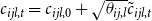 $c_{ijl,t} = c_{ijl,0} + \sqrt{\theta_{ij,l}} \tilde{c}_{ijl,t}$
yields the corresponding state equation
$c_{ijl,t} = c_{ijl,0} + \sqrt{\theta_{ij,l}} \tilde{c}_{ijl,t}$
yields the corresponding state equation
 \begin{equation*}\tilde{\textbf{C}}_{ij,t} = \tilde{\textbf{C}}_{ij,t-1} + \textbf{v}_t, \quad \textbf{v}_t\sim\mathcal{N}(\textbf{0},\textbf{I}_{\tilde{K}}),\end{equation*}
with
 $\tilde{\textbf{C}}_{ij,0} = \textbf{0}_{\tilde{K}}$
. This procedure moves the square root of the innovation variances to the states into equation (5). The resulting representation has the property that the
$\tilde{\textbf{C}}_{ij,0} = \textbf{0}_{\tilde{K}}$
. This procedure moves the square root of the innovation variances to the states into equation (5). The resulting representation has the property that the
 $\sqrt{\theta_{ij,l}}$
’s can be treated as regression coefficients.
$\sqrt{\theta_{ij,l}}$
’s can be treated as regression coefficients.
2.3 Prior distributions
The parameter space of the proposed model is high-dimensional. Consequently, I use Bayesian methods for estimation and inference to impose shrinkage. Before proceeding, I stack the coefficients using
 $\textbf{c}_{i} = \text{vec}(\textbf{C}_{i1,0}^{\prime},\ldots,\textbf{C}_{ik,0}^{\prime})$
, collect the square roots of the innovation variances
$\textbf{c}_{i} = \text{vec}(\textbf{C}_{i1,0}^{\prime},\ldots,\textbf{C}_{ik,0}^{\prime})$
, collect the square roots of the innovation variances
 $\sqrt{\theta_{ij,l}}$
in
$\sqrt{\theta_{ij,l}}$
in
 $\sqrt{{\boldsymbol\theta}_i} = (\sqrt{\theta_{i1,1}},\ldots,\sqrt{\theta_{i1,\tilde{K}}},\ldots,\sqrt{\theta_{ik,1}},\ldots,\sqrt{\theta_{ik,\tilde{K}}})'$
, and index the jth elements by
$\sqrt{{\boldsymbol\theta}_i} = (\sqrt{\theta_{i1,1}},\ldots,\sqrt{\theta_{i1,\tilde{K}}},\ldots,\sqrt{\theta_{ik,1}},\ldots,\sqrt{\theta_{ik,\tilde{K}}})'$
, and index the jth elements by
 $c_{ij}$
and
$c_{ij}$
and
 $\sqrt{\theta_{ij}}$
, respectively, with
$\sqrt{\theta_{ij}}$
, respectively, with
 $j=1,\ldots,k\tilde{K}$
. I propose to use a horseshoe (HS) prior (see Carvalho et al. (Reference Carvalho, Polson and Scott2010)) on various parts of the parameter space to achieve regularization, thereby selecting important domestic and cross-country coefficients while shrinking unimportant ones to zero. The HS is chosen due to its excellent theoretical and empirical shrinkage properties and its simplicity, since it has no additional tuning or hyperparameters.Footnote 10
$j=1,\ldots,k\tilde{K}$
. I propose to use a horseshoe (HS) prior (see Carvalho et al. (Reference Carvalho, Polson and Scott2010)) on various parts of the parameter space to achieve regularization, thereby selecting important domestic and cross-country coefficients while shrinking unimportant ones to zero. The HS is chosen due to its excellent theoretical and empirical shrinkage properties and its simplicity, since it has no additional tuning or hyperparameters.Footnote 10
For the constant part of the coefficients, the HS prior is given by:
 \begin{equation*}c_{ij}|\mu_{cj},\tau_{cj},\lambda_c\sim\mathcal{N}(\mu_{cj},\tau_{cij}^2\lambda_c^2), \quad \tau_{cij}\sim\mathcal{C}^{+}(0,1), \quad \lambda_{c}\sim\mathcal{C}^{+}(0,1),\end{equation*}
with
 $\mathcal{C}^{+}(\bullet)$
referring to the half-Cauchy distribution. The country-specific coefficients are pushed towards the prior mean
$\mathcal{C}^{+}(\bullet)$
referring to the half-Cauchy distribution. The country-specific coefficients are pushed towards the prior mean
 $\mu_{cj}$
. The prior mean
$\mu_{cj}$
. The prior mean
 $\mu_{cj}=0$
for all coefficients. It is worth mentioning that one may set specific elements
$\mu_{cj}=0$
for all coefficients. It is worth mentioning that one may set specific elements
 $\mu_{cj}=1$
(e.g. those associated with the first own lag of the respective endogenous variable per equation) to mimic a conventional Minnesota-type prior. The overall degree of shrinkage is determined by a global shrinkage parameter
$\mu_{cj}=1$
(e.g. those associated with the first own lag of the respective endogenous variable per equation) to mimic a conventional Minnesota-type prior. The overall degree of shrinkage is determined by a global shrinkage parameter
 $\lambda_{c}$
serving as a general indicator of sparsity pooled over the cross-section and variable types. Flexibility for individual coefficients is provided by local scaling parameters
$\lambda_{c}$
serving as a general indicator of sparsity pooled over the cross-section and variable types. Flexibility for individual coefficients is provided by local scaling parameters
 $\tau_{cij}$
.
$\tau_{cij}$
.
Shrinkage on the innovation variances of the states in equation (4) is introduced in similar vein. Frühwirth-Schnatter and Wagner (Reference Frühwirth-Schnatter and Wagner2010) show that a Gamma prior on the state innovation variances is equivalent to imposing a Gaussian prior on their square root:
 \begin{equation*}\sqrt{\theta_{ij}}|\tau_{\theta ij},\lambda_{\theta}\sim\mathcal{N}(0,\tau_{\theta ij}^2\lambda_{\theta}^2), \quad \tau_{\theta ij}\sim\mathcal{C}^{+}(0,1), \quad \lambda_{\theta}\sim\mathcal{C}^{+}(0,1).\end{equation*}
All variances are pushed towards zero a priori. This feature selects which coefficients are constant, and which of them vary over time. The global parameter
 $\lambda_{\theta}$
again pools information about sparsity over the cross-section and variable types, while the local scalings
$\lambda_{\theta}$
again pools information about sparsity over the cross-section and variable types, while the local scalings
 $\tau_{\theta ij}$
are variable- and country-specific.
$\tau_{\theta ij}$
are variable- and country-specific.
It remains to specify prior distributions on the factor loadings in
 $\textbf{L}$
. I stack the free elements in a vector
$\textbf{L}$
. I stack the free elements in a vector
 $\textbf{l}$
with typical element
$\textbf{l}$
with typical element
 $l_j$
for
$l_j$
for
 $j=1,\ldots,R\ (R=Kd-[d(d+1)/2])$
and impose
$j=1,\ldots,R\ (R=Kd-[d(d+1)/2])$
and impose
 \begin{equation*}l_{j}|\tau_{Lj},\lambda_L\sim\mathcal{N}(0,\tau_{Lj}^2\lambda_{L}^2), \quad \tau_{Lj}\sim\mathcal{C}^{+}(0,1), \quad \lambda_L\sim\mathcal{C}^{+}(0,1).\end{equation*}
Chan (Reference Chan2021) notes that choosing underfitting factor models carries a much larger penalty than using an overfitting specification in terms of model selection criteria. Consequently, it is possible to set the number of factors d to a comparatively large value, and the shrinkage prior on the factor loadings serves to achieve a data-driven selection of an adequate number of factors, see also Kastner (Reference Kastner2019).
The state innovation variance for the common volatility process of
 $h_t$
is assigned an inverse Gamma prior distribution, with
$h_t$
is assigned an inverse Gamma prior distribution, with
 $\sigma_h^2\sim\mathcal{G}^{-1}(\mathfrak{a},\mathfrak{b})$
. The hyperparameters
$\sigma_h^2\sim\mathcal{G}^{-1}(\mathfrak{a},\mathfrak{b})$
. The hyperparameters
 $\mathfrak{a}$
and
$\mathfrak{a}$
and
 $\mathfrak{b}$
are chosen such that the prior has a mean of
$\mathfrak{b}$
are chosen such that the prior has a mean of
 $0.2$
with variance 1. For the idiosyncratic stochastic volatility innovation variances, I choose a set of independent Gamma priors,
$0.2$
with variance 1. For the idiosyncratic stochastic volatility innovation variances, I choose a set of independent Gamma priors,
 $\sigma_{\omega ij}^2\sim\mathcal{G}(1/2,1/2)$
. Using a Gamma rather than an inverse Gamma prior has the advantage that no mass is bound away from zero a priori. This specification corresponds to a Gaussian prior on
$\sigma_{\omega ij}^2\sim\mathcal{G}(1/2,1/2)$
. Using a Gamma rather than an inverse Gamma prior has the advantage that no mass is bound away from zero a priori. This specification corresponds to a Gaussian prior on
 $\sigma_{\omega ij}$
with zero mean and unit variance, see Frühwirth-Schnatter and Wagner (Reference Frühwirth-Schnatter and Wagner2010). The independent prior models for the idiosyncratic stochastic volatilities are thus centered on the homoscedastic case.
$\sigma_{\omega ij}$
with zero mean and unit variance, see Frühwirth-Schnatter and Wagner (Reference Frühwirth-Schnatter and Wagner2010). The independent prior models for the idiosyncratic stochastic volatilities are thus centered on the homoscedastic case.
2.4 Posterior simulation
Full conditional posterior distributions obtained from combining the likelihood function with the priors and the corresponding estimation algorithm are discussed in detail in Appendices A and B. Most distributions are of well-known form, allowing for a simple Markov chain Monte Carlo (MCMC) algorithm to obtain draws from the joint posterior using a Gibbs sampler.
The full history of the TVPs can be drawn by using a FFBS algorithm (Carter and Kohn (Reference Carter and Kohn1994); Frühwirth-Schnatter (Reference Frühwirth-Schnatter1994)). A similar algorithm is employed for the idiosyncratic stochastic volatilities, conditional on a mixture approximation of the corresponding state, and measurement equations (see Kim et al. (Reference Kim, Shephard and Chib1998)). This mixture approximation is inapplicable for sampling the stochastic volatility path of the common factors due to the presence of this volatility in the mean of the measurement equation. Here, I use a random walk Metropolis–Hastings algorithm as an alternative (see also Jacquier et al. (Reference Jacquier, Polson and Rossi2002)).
3. Data and model specification
The dataset consists of monthly data for the period ranging from 1995:01 to 2019:12 for the G7 economies: Canada (CA), France (FR), Germany (DE), Italy (IT), Japan (JP), the United Kingdom (UK), and the USA.Footnote 11 The set of endogenous variables by country is dictated by the requirement of consistent availability over time and the cross-section, and patterned to provide a realistic probabilistic model of domestic and international macroeconomic dynamics.
In terms of the real economy, the dataset features series on industrial production (INP, as monthly indicator of economic activity), the unemployment rate (UNR) and year-on-year consumer price inflation (CPI). Motivated by recent findings on the importance of financial conditions in the transmission of uncertainty shocks (see, e.g. Alessandri and Mumtaz (Reference Alessandri and Mumtaz2019)) and the overall importance of the financial sector for the real economy, this set is extended with several financial quantities. I include short-term (SIR) and long-term interest rates (LIR) based on their importance for the conduct of both conventional and unconventional monetary policy by central banks, and to reflect changes in borrowing conditions in light of international finance. Moreover, I use equity prices (EQP) and a measure of overall financial/credit market conditions (FCI). The FCI measure is included based on a recent strand of literature focusing on potentially nonlinear effects of financial stress on economic activity, which is linked to episodes of uncertainty (see Adrian et al. (Reference Adrian, Boyarchenko and Giannone2019)).
INP and EQP enter the model in natural logarithms (to be interpreted as percent). UNR, year-on-year CPI, SIR, and LIR are included in levels (to be interpreted as percentage points). The data except the FCI’s are downloaded from the FRED database of the Federal Reserve Bank of St. Louis (online at fred.stlouisfed.org), which collects them from the OECD’s main economic indicator database. As financial stress measures, I use the composite indicator of systemic stress for the continental European economies and the UK provided by the European Central Bank, the Federal Reserve Bank of Chicago National Financial Conditions Index for the USA, the Canadian Financial Stress Index for Canada, and the Japan Center for Economic Research Financial Stress Index for Japan. To make the scales of these indices comparable, they are standardized such that their range lies in the unit interval prior to estimation (i.e. zero and one mean minimal and maximal financial stress over the sampling period, respectively). To construct the cross-sectional weights for establishing links between economies, I rely on bilateral annual trade flows averaged over the sample period.
A chart of the included variables is provided in Appendix D. All data are standardized to have zero mean and unit variance prior to estimation to avoid numerical instabilities from different scalings. The impulse responses are transformed back to the original scale afterwards. All dimensions of the involved vectors are given based on
 $k=7$
and
$k=7$
and
 $N=7$
. I choose
$N=7$
. I choose
 $P=Q=3$
lags and
$P=Q=3$
lags and
 $d=15$
factors. Varying the number of factors and lags and re-estimating the model over a grid does not qualitatively alter the results. This suggests that the shrinkage priors perform well for selecting important parameters from an a priori overfitting specification.
$d=15$
factors. Varying the number of factors and lags and re-estimating the model over a grid does not qualitatively alter the results. This suggests that the shrinkage priors perform well for selecting important parameters from an a priori overfitting specification.
4. Empirical results
4.1 The measure of uncertainty
The resulting posterior median estimate of uncertainty alongside 50 and 68% posterior credible sets is shown in Figure 1. The vertical lines indicate events commonly associated with uncertainty shocks. These events are the 1997 Asian financial crisis, the Russian crisis, and the bankruptcy of the hedge fund Long-Term Capital Management (LTCM) in late 1998, the burst of the dot-com bubble in early 2000 (which saw substantial stock market declines following a bullish market for technology related equities), the 9/11 terror attacks in September 2001 and the subsequent Gulf War II in 2003. Moreover, I indicate the collapse of the US investment bank Lehman Brothers at the onset of the global financial crisis in late 2008 and the European sovereign debt crisis mid 2011. I also indicate the European immigration crisis which reached its peak in 2015. The final uncertainty-related events are the Brexit referendum and the election of Donald J. Trump as 45th president of the USA in mid/late 2016.
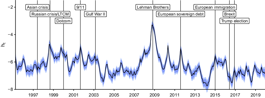
Fig. 1. The uncertainty measure
 $h_t$
. Notes: The solid black line depicts the posterior median estimate of the uncertainty measure over time. The blue shaded areas refer to the 50% and 68% posterior credible sets. The vertical lines indicate events commonly associated with uncertainty shocks.
$h_t$
. Notes: The solid black line depicts the posterior median estimate of the uncertainty measure over time. The blue shaded areas refer to the 50% and 68% posterior credible sets. The vertical lines indicate events commonly associated with uncertainty shocks.
Inspecting Figure 1 in more detail, it is worth mentioning that there are periods of persistently high and low uncertainty, but with several high-frequency spikes. High-uncertainty episodes are present between 1999 and 2003, and 2007 and 2009. The first period is characterised mainly by the occurrence of many uncertainty-related events. Three of these events are of financial nature: the 1997 Asian crisis, the Russian crisis and subsequent collapse of LTCM and the burst of the dot-com bubble. On the other hand, the 9/11 terror attacks materialize as a prominent local peak, while Gulf War II appears as a more gradual and slightly more persistent uncertainty episode. Following this tumultuous period, between 2004 and 2007, international uncertainty is at a comparatively low level. Initial increases associated with the second high-uncertainty period surrounding the global financial crisis emerged in late 2007.
The measure peaks in September 2008, coinciding with the collapse of Lehman Brothers. This global maximum is in line with expectations. Troubling dynamics in the US financial sector spilled over to the real economy across countries, simultaneously provoking a set of counteracting policy measures—thereby affecting both real and financial quantities resulting in substantial comovements in all endogenous variables. Uncertainty declined after 2009. However, there are two local peaks in late 2010 and early 2011, associated with the emergence of the European sovereign debt crisis. The lowest level of uncertainty is detected around 2014. Afterwards, shocks and high levels of uncertainty appear around the European immigration crisis around 2015, the Brexit referendum and the 2016 US presidential election. Until the end of the sample, I detect several high-frequency spikes, which can be linked to tensions in US/China trade relations.
Figure 2 offers a comparison of my endogenous measure of uncertainty with several prominent proxies in the literature. This exercise serves to identify commonalities and differences with respect to the econometric measurement of uncertainty rather than using alternatives such as the newspaper-based approaches. In particular, I consider the geopolitical risk (GPR) index described in Caldara and Iacoviello (Reference Caldara and Iacoviello2018), the global policy uncertainty (GEPU) and the world uncertainty index (WUI). The latter index is provided in several variants. I use the global index (averaged across all countries), the corresponding measure using weights reflecting the countries’ contribution to global GDP, and an average measure tracking only advanced economies.Footnote 12
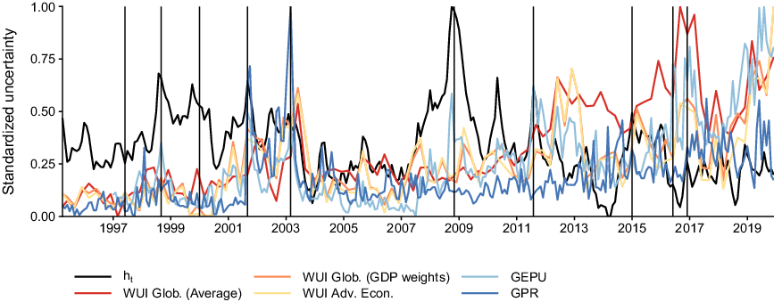
Fig. 2. Comparison of international uncertainty measures. Notes: To make the measures comparable in scale, I standardize all uncertainty measures to lie in the unit interval by subtracting the respective minimum and dividing by the maximum value over time. The solid black line shows the posterior median estimate of
 $h_t$
. Other uncertainty measures are geopolitical risk (GPR), global policy uncertainty (GEPU), and variants of the world uncertainty index (WUI). The vertical lines indicate events commonly associated with uncertainty shocks.
$h_t$
. Other uncertainty measures are geopolitical risk (GPR), global policy uncertainty (GEPU), and variants of the world uncertainty index (WUI). The vertical lines indicate events commonly associated with uncertainty shocks.
Comovements of the endogenous measure are apparent particularly with GEPU, with many peaks coinciding. This provides empirical evidence that the proposed measure captures a diverse set of uncertainty-related aspects with respect to economic policy. The least association is apparent with the GRP index (particularly during the period from 2007 to 2013), which can be explained by noting that this index mainly tracks political events such as military-related, nuclear, or war and terror-related threats. However, I find that particularly the peaks associated with such events (e.g. the 9/11 terror attacks and Gulf War II) are accurately captured in
 $h_t$
. These findings are reassuring, given that I intend to provide a measure of uncertainty in line with the JLN definition, which captures uncertainty not only in a selected number of cases, but one that is common to many economic and financial series and based on the unforecastable component of these variables.
$h_t$
. These findings are reassuring, given that I intend to provide a measure of uncertainty in line with the JLN definition, which captures uncertainty not only in a selected number of cases, but one that is common to many economic and financial series and based on the unforecastable component of these variables.
Perhaps more interestingly, there are at least two key differences between the newspaper-based approach to measuring uncertainty and its econometric measurement. First, none of the proxies detects uncertainty during the period from 1997 to 2001 which comprises several events that are commonly associated with uncertainty shocks. Second, all proxies show upward trending behavior towards the end of the sample. While high-frequency dynamics between
 $h_t$
and the other indices often are comparable,
$h_t$
and the other indices often are comparable,
 $h_t$
lacks such low frequency movements. These empirical features of the estimated
$h_t$
lacks such low frequency movements. These empirical features of the estimated
 $h_t$
are in line with similar econometric approaches to measuring uncertainty. Indeed, the measure obtained in this study shows roughly the same dynamics as those in Carriero et al. (Reference Carriero, Clark and Marcellino2020) or Mumtaz and Musso (Reference Mumtaz and Musso2019). This finding provides evidence for the robustness of the results in earlier econometric papers—the proposed model is more flexible and offers several novel inferential possibilities such as assessing time variation in impulse responses and tracing the effects of an uncertainty shock in a multi-country model; however, key dynamics of the uncertainty measure are robust to these extensions.
$h_t$
are in line with similar econometric approaches to measuring uncertainty. Indeed, the measure obtained in this study shows roughly the same dynamics as those in Carriero et al. (Reference Carriero, Clark and Marcellino2020) or Mumtaz and Musso (Reference Mumtaz and Musso2019). This finding provides evidence for the robustness of the results in earlier econometric papers—the proposed model is more flexible and offers several novel inferential possibilities such as assessing time variation in impulse responses and tracing the effects of an uncertainty shock in a multi-country model; however, key dynamics of the uncertainty measure are robust to these extensions.
I conjecture that the differences between proxies and the econometric measurement of uncertainty in line with the JLN definition, particularly after 2011, are due to the following reasons. First, uncertainty has received a substantial amount of attention from policymakers after the Great Recession. In conjunction with the explosion of uncertainty-related research following Bloom (Reference Bloom2009), this may have resulted in increased public and media awareness of the role of uncertainty in policy decisions and business cycle fluctuations. Consequently, this increased awareness may be reflected also in newspaper articles, which proxies in the spirit of Baker et al. (Reference Baker, Bloom and Davis2016) are based upon, thereby “endogenously” increasing mentions of uncertainty related keywords and the corresponding index. However, the period starting 2016 has arguably been tumultuous and featured many potential uncertainty shocks. Thus, it is perhaps an impossible task to isolate and decompose such dynamics. Second, the JLN definition requires uncertainty measure to be based on the purely unforecastable component of an economic or financial variable. While it may well be the case that the overall level of uncertainty has increased since 2016, economic agents likely adjusted their expectations to this. The proposed model reflects this by including the contemporaneous measure of uncertainty, which informs the forecasts of all other endogenous variables. When uncertainty has predictive power, which several papers suggest to be the case, this decreases the unforecastable component in magnitude, and thereby also its volatility (which is the measure of uncertainty). The proxies do not have this property.
4.2 Comparing domestic and international measures of uncertainty
The previous subsection discusses the international measure of uncertainty and compares it to several proxies. In the following, I further extend this discussion and assess comovements and differences between country-specific econometric measures of uncertainty and international uncertainty. For this purpose, I obtain an uncertainty measure,
 $h_{it}$
, using the proposed model framework by country (ruling out static and dynamic interdependencies) for countries
$h_{it}$
, using the proposed model framework by country (ruling out static and dynamic interdependencies) for countries
 $i=1,\ldots,N$
. For specifics of the country-specific VAR models, see Appendix C. Note that using the identified factor model allows for a one-to-one comparison of domestic and international uncertainty with respect to its level in a way that other approaches using proxies cannot.
$i=1,\ldots,N$
. For specifics of the country-specific VAR models, see Appendix C. Note that using the identified factor model allows for a one-to-one comparison of domestic and international uncertainty with respect to its level in a way that other approaches using proxies cannot.
The first set of results is summarized in the form of a correlation matrix in Table 1. The strongest comovement of international with domestic uncertainty is present for France and the USA. Pairwise correlations are highly statistically significant, and have a correlation coefficient of about
 $0.7$
. Correlations are also high for the cases of Germany, Japan, and the UK. Domestic uncertainty in Canada is only modestly related to international uncertainty, with a correlation of
$0.7$
. Correlations are also high for the cases of Germany, Japan, and the UK. Domestic uncertainty in Canada is only modestly related to international uncertainty, with a correlation of
 $0.11$
. The most interesting case is Italy, with a statistically significant negative correlation to the international measure. I discuss the sources of this disconnect below when assessing differences of domestic and international uncertainty over time.
$0.11$
. The most interesting case is Italy, with a statistically significant negative correlation to the international measure. I discuss the sources of this disconnect below when assessing differences of domestic and international uncertainty over time.
Table 1. Correlation of international uncertainty and country-specific uncertainty.
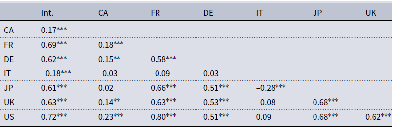
Notes: Pairwise correlation matrix of the posterior medians of country-specific uncertainty measures
 $h_{it}$
and
$h_{it}$
and
 $h_t$
. ‘Int.’ refers to the international measure
$h_t$
. ‘Int.’ refers to the international measure
 $h_t$
, country-codes indicate country-specific measures
$h_t$
, country-codes indicate country-specific measures
 $h_{it}$
for
$h_{it}$
for
 $i\in\{\text{US,CA,UK,DE,FR,IT}\}$
. Statistical significance is indicated by asterisks, p-values:
$i\in\{\text{US,CA,UK,DE,FR,IT}\}$
. Statistical significance is indicated by asterisks, p-values:
 $^{*}<0.1$
,
$^{*}<0.1$
,
 $^{**}<0.05$
and
$^{**}<0.05$
and
 $^{***}<0.01$
.
$^{***}<0.01$
.
In terms of domestic correlations, several interesting patterns are noteworthy. Canadian uncertainty exhibits the largest and statistically significant correlation with the USA, albeit measured at a comparatively low
 $0.23$
. Uncertainty in Germany and France exhibits substantial comovement. While the correlation between Germany and France is largest from a German perspective, French uncertainty has the highest pairwise correlation with the domestic measure for the USA. Interestingly, the UK uncertainty measure is most correlated with Japanese uncertainty. The maximum correlation between two domestic measures is the one between USA and French uncertainty. Interestingly, Italian uncertainty shows a statistically significantly negative correlation with Japan at
$0.23$
. Uncertainty in Germany and France exhibits substantial comovement. While the correlation between Germany and France is largest from a German perspective, French uncertainty has the highest pairwise correlation with the domestic measure for the USA. Interestingly, the UK uncertainty measure is most correlated with Japanese uncertainty. The maximum correlation between two domestic measures is the one between USA and French uncertainty. Interestingly, Italian uncertainty shows a statistically significantly negative correlation with Japan at
 $-0.28$
, and those with other domestic measures are either slightly positive or negative but all insignificant.
$-0.28$
, and those with other domestic measures are either slightly positive or negative but all insignificant.
To assess when differences in domestic and international uncertainty occur, the left panels of Figure 3 show the posterior median of the country-specific uncertainty measure
 $h_{it}$
alongside 50% and 68% posterior credible sets in blue. The 68% posterior credible set of the international uncertainty measure
$h_{it}$
alongside 50% and 68% posterior credible sets in blue. The 68% posterior credible set of the international uncertainty measure
 $h_t$
is depicted as grey-shaded area. The right panel shows the posterior distribution of the difference between domestic and international uncertainty,
$h_t$
is depicted as grey-shaded area. The right panel shows the posterior distribution of the difference between domestic and international uncertainty,
 $h_{it}-h_{t}$
. Positive values indicate that domestic uncertainty was higher than international uncertainty in the respective periods and vice versa.
$h_{it}-h_{t}$
. Positive values indicate that domestic uncertainty was higher than international uncertainty in the respective periods and vice versa.
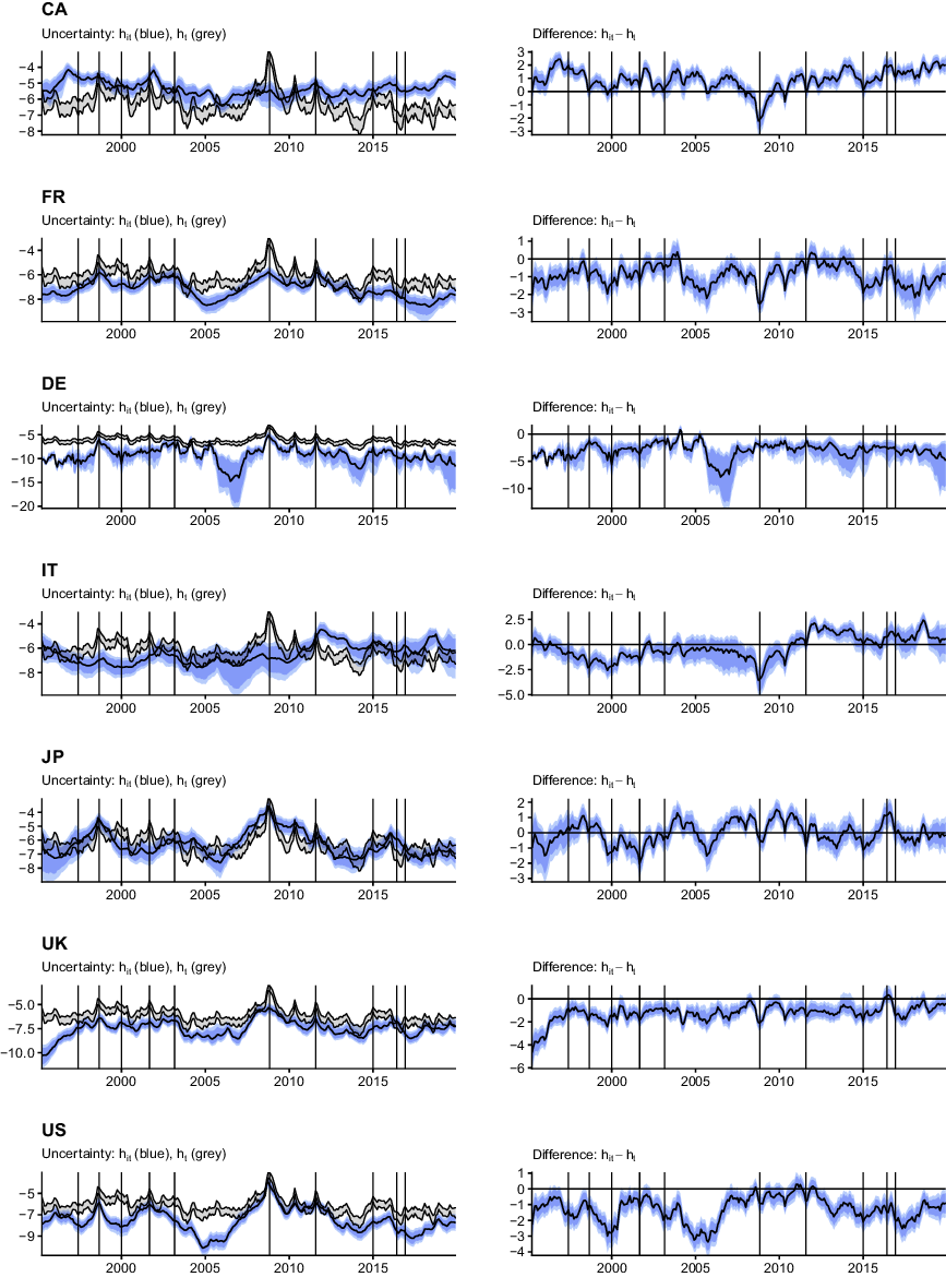
Fig. 3. Differences between country-specific and international uncertainty. Notes: The left panels show the posterior median of the country-specific uncertainty measure
 $h_{it}$
alongside 50 and 68% posterior credible sets in blue. The posterior 68% credible set of the international uncertainty measure
$h_{it}$
alongside 50 and 68% posterior credible sets in blue. The posterior 68% credible set of the international uncertainty measure
 $h_t$
is depicted as grey area. The right panel shows the posterior distribution of the difference between domestic and international uncertainty,
$h_t$
is depicted as grey area. The right panel shows the posterior distribution of the difference between domestic and international uncertainty,
 $h_{it}-h_{t}$
. Positive values indicate domestic uncertainty was higher than international uncertainty in the respective periods and vice versa.
$h_{it}-h_{t}$
. Positive values indicate domestic uncertainty was higher than international uncertainty in the respective periods and vice versa.
Figure 3 shows significant differences between both the level and dynamics of the international versus domestic uncertainty measure. Moreover, I detect a substantial amount of heterogeneity over the cross-section. The preceding analysis of pairwise correlations indicates that comovement between the domestic and international measure is most pronounced for the USA, UK, Germany, France, and Japan. The domestic measures for these countries reflect most peaks and troughs in the international metric. Canada, and Italy in particular, however, exhibit striking differences.
The most prominent difference for these two countries is present around the Great Recession. Domestic uncertainty increases moderately during this period in both Canada and Italy, but far from the increases visible in the international measure or the other domestic metrics. Interestingly, Canadian uncertainty is higher than international uncertainty for most of the sample (the right panel of the figure indicates a significant positive difference). Such positive differences for Canada are most pronounced early in the sample, during the comparatively calm economic period between 2005 and the Great Recession, and at the end of the sample. It is worth mentioning that these patterns are roughly in line with domestic newspaper-based measures of uncertainty. The peak difference towards the end of the sample coincides with the Brexit referendum, and is economically reasonable since the UK is an important trade partner of Canada. For Italy, differences are less systematic. Notable country-specific peaks are present during the European sovereign debt crisis, which appears reasonable with Italy being affected severely due to high precrisis government debt levels. An interesting episode for Italy is visible during the late 1990s and early 2000s, where Italian uncertainty is consistently lower than the international measure.
Turning to the economies where domestic uncertainty exhibits higher correlations with the international measure, several findings are worth noting. First, apart from Japan, all other countries typically show statistically significantly lower levels of domestic uncertainty, with a minor number of positive differences (that are insignificant in all cases). Largest (negative) differences materialize in Germany, particularly during the tranquil period between 2005 and the Great Recession. A similar pattern is visible for the case of the USA, albeit with smaller differences. In addition, domestic uncertainty in the USA around 2000 (the burst of the dotcom-bubble) is lower than the international measure. This can be explained by the domestic VAR classifying the collapse of technology-related stock prices as an idiosyncratic financial shock rather than an economy-wide phenomenon. By contrast, linkages in international financial markets result in elevated international uncertainty when using the GVAR framework. Another country-specific increase in uncertainty worth mentioning for the UK is the one occurring around the Brexit referendum. A different pattern over time is visible in Japan. Early in the sample, during the 1997 Asian financial crisis, domestic Japanese uncertainty is higher than international uncertainty, which can be explained by the closer geographic and economic proximity of Japan with the countries primarily affected by this crisis. Interestingly, Japan also exhibits higher uncertainty compared to the international measure just prior to the peak of the European sovereign debt crisis and around the Brexit referendum.
Summing up, while many peaks between econometric and proxy measures of uncertainty coincide (depending on the respective index), there are pronounced differences particularly towards more recent periods. Moreover, I detect substantial differences between several domestic measures and international uncertainty. These differences not only concern both the level of uncertainty, but also idiosyncratic dynamics. These findings corroborate and extend those of preceding econometric studies with respect to country coverage and by enabling a direct comparison of domestic and international uncertainty.
4.3 Dynamic responses to uncertainty shocks
The previous section is concerned with discussing empirical features of the proposed approach to measuring uncertainty. In the following, I discuss the macroeconomic and financial consequences of shocks to the international measure of uncertainty. It is worth reiterating that the proposed TVP-GVAR-FSVM provides a probabilistic measure of uncertainty, thereby allowing for more accurate inference compared to proxy-based two-stage approaches. Moreover, the model takes international spillovers and higher order effects across countries into account. Earlier papers focused mainly on a few key indicators such as output growth. The results discussed in the following provide a more nuanced empirical characterization of the macroeconomic and financial effects of uncertainty shocks. Figure 4 shows the posterior median of cumulative 1-year ahead responses across countries and variable types, alongside 50% posterior credible intervals. Additional empirical results such as posterior median impulse responses over time for an impulse response horizon up to 36 months (3 years) and other horizons for the cumulative responses are provided in Appendix D.
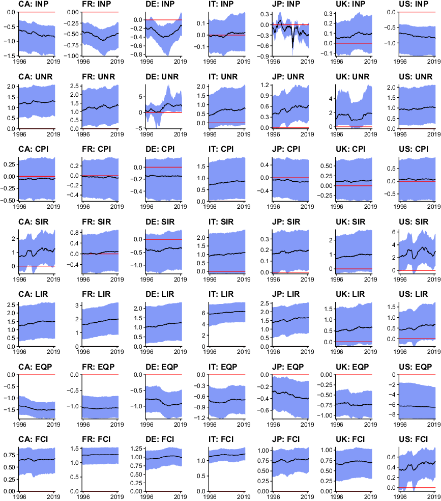
Fig. 4. Cumulative one-year ahead response to an international uncertainty shock. Notes: The solid red horizontal line marks zero, the solid black line is the posterior median estimate of the cumulative one-year ahead response. The blue shaded area covers the 50% posterior credible interval.
From an econometric perspective, it is worth mentioning that most parts of the parameter space are shrunk heavily towards time-invariant parameters, with some exceptions. This appears sensible for a model of this size. Notable examples for responses featuring abrupt changes over time are UNRs, SIRs, and INP for some countries, while I detect minor gradual adjustments for EQPs. While some variables exhibit time-varying behavior on impact (captured by
 ${\boldsymbol\beta}_{it}$
), the shapes of impulse responses also exhibit signal-varying degrees of persistence of the shock. In addition to heterogeneity over time, a substantial degree of heterogeneity over the cross-section is present. These empirical findings emphasize the need for sophisticated econometric methods. Using, for instance, a conventional panel VAR with a cross-sectional homogeneity restriction would produce an average response across countries, which clearly misses nuanced country-specific dynamics. Moreover, disregarding time variation not only would affect both the measure of uncertainty (by disregarding parameter change that helps producing a more accurate unforecastable component required by the definition of uncertainty), but also would result in a time average of the impulse responses that neglects changes in the impact and persistence of the shocks. In what follows, I discuss impulse response functions by variable type.
${\boldsymbol\beta}_{it}$
), the shapes of impulse responses also exhibit signal-varying degrees of persistence of the shock. In addition to heterogeneity over time, a substantial degree of heterogeneity over the cross-section is present. These empirical findings emphasize the need for sophisticated econometric methods. Using, for instance, a conventional panel VAR with a cross-sectional homogeneity restriction would produce an average response across countries, which clearly misses nuanced country-specific dynamics. Moreover, disregarding time variation not only would affect both the measure of uncertainty (by disregarding parameter change that helps producing a more accurate unforecastable component required by the definition of uncertainty), but also would result in a time average of the impulse responses that neglects changes in the impact and persistence of the shocks. In what follows, I discuss impulse response functions by variable type.
Industrial production (INP). Related studies usually find strong decreases of economic activity (measured in this paper by INP as a monthly indicator) following an uncertainty shock. My results signal that this depends on the respective country. The time profile of the cumulative response for the USA and Canada is roughly comparable, with an uncertainty shock decreasing INP between
 $0.5\%$
and 1% after 1 year. The responses indicate that the effects of uncertainty shocks increase over time, contrary to the findings of Mumtaz and Theodoridis (Reference Mumtaz and Theodoridis2017) for the case of the USA. This empirical finding points towards the importance of considering international information in a multi-country model, and decreases in the effects of uncertainty shocks may be an artefact of omitted variable bias in small domestic information sets. The responses for Germany and France show a similar pattern over time, with smaller negative effects early and late in the sample, but pronounced decreases in INP around the European sovereign debt crisis. Interestingly, the responses for the UK and Italy are insignificant. This finding can be explained by closer inspection of the shapes of the impulse responses using the results in Appendix D. The impact response in both countries is negative, but there is a strong rebound after several months. The response for Japan shows substantial and abrupt movements over time. While responses during the Asian financial crisis of 1997 and the Great Recession are substantial and negative, there are periods of insignificant 1-year ahead responses. Effects tend to become stronger towards the end of the sample.
$0.5\%$
and 1% after 1 year. The responses indicate that the effects of uncertainty shocks increase over time, contrary to the findings of Mumtaz and Theodoridis (Reference Mumtaz and Theodoridis2017) for the case of the USA. This empirical finding points towards the importance of considering international information in a multi-country model, and decreases in the effects of uncertainty shocks may be an artefact of omitted variable bias in small domestic information sets. The responses for Germany and France show a similar pattern over time, with smaller negative effects early and late in the sample, but pronounced decreases in INP around the European sovereign debt crisis. Interestingly, the responses for the UK and Italy are insignificant. This finding can be explained by closer inspection of the shapes of the impulse responses using the results in Appendix D. The impact response in both countries is negative, but there is a strong rebound after several months. The response for Japan shows substantial and abrupt movements over time. While responses during the Asian financial crisis of 1997 and the Great Recession are substantial and negative, there are periods of insignificant 1-year ahead responses. Effects tend to become stronger towards the end of the sample.
Unemployment rate (UNR). Turning to the UNR, I detect a substantial degree of heterogeneity over the cross-section and over time. Interestingly, while the unemployment responses for the USA, Canada, and France are roughly constant over time, this is not the case in the UK, Germany, and Japan. An international uncertainty shock increases the UNR in the former three countries by approximately one percentage point. While responses for Italy are similar in size, they are insignificant throughout the sampling period. The magnitudes of the responses for Japan, on the other hand, are much smaller, and insignificant early in the sample. In the UK, I detect distinct periods of large and small effects. Labor markets in the UK were less affected in the period surrounding the Great Recession, with cumulative 1-year ahead responses of about one percentage point (in line with the other countries). Earlier in the sample, and after the Great Recession, the corresponding effects are almost two percentage points. Another interesting case is Germany. The responses are insignificant early in the sample, but range up to
 $2.5$
percentage points after 2005. This increase in the effects of uncertainty shocks coincides with changes in legislation in Germany resulting in less rigid labor markets after 2005, which clearly affects the transmission of international uncertainty.
$2.5$
percentage points after 2005. This increase in the effects of uncertainty shocks coincides with changes in legislation in Germany resulting in less rigid labor markets after 2005, which clearly affects the transmission of international uncertainty.
Consumer price inflation (CPI). The cumulative 1-year responses are insignificant for all countries apart from Italy. This finding can be explained by two counteracting forces identified in the structural model developed by Fernández-Villaverde et al. (Reference Fernández-Villaverde, Guerrón-Quintana, Kuester and Rubio-Ramírez2015). The channels are, on the one hand, the aggregate demand channel, which states that households reduce consumption after an uncertainty shock and thereby put downward pressure on prices. On the other hand, there is also the upward-pricing bias channel, which yields increases in inflation based on profit maximization concerns by firms. The empirical response is thus a mixture of these two counteracting forces, and their relative strength is determined by the respective demand elasticity in a given country and the stickiness of prices. For the case of Italy, the upward-pricing channel clearly dominates (indicating comparatively flexible prices), with cumulative increases in inflation of about
 $0.75$
percentage points after 1 year. Albeit the response is insignificant, the aggregate demand channel appears to be stronger in the case of Germany, with some posterior mass of the responses shifted towards lower prices. For the other countries, the 1-year cumulative responses are closely centered on zero. Regarding time variation, my findings indicate that the effects of uncertainty on consumer prices are rather constant over time.
$0.75$
percentage points after 1 year. Albeit the response is insignificant, the aggregate demand channel appears to be stronger in the case of Germany, with some posterior mass of the responses shifted towards lower prices. For the other countries, the 1-year cumulative responses are closely centered on zero. Regarding time variation, my findings indicate that the effects of uncertainty on consumer prices are rather constant over time.
Interest rates (SIR/LIR). I measure statistically significant increases in long-term rates for all countries apart from the UK. In this case, there may again be two counteracting forces. First, debt-financed fiscal policy measures targeting contractionary effects of international uncertainty shocks increase the amount of government debt, which implies higher interest rates on bonds. Second, investors typically resort to safer assets in times of uncertainty, where increased demand lowers prices and thus increases rates (see, e.g. Caballero et al. (Reference Caballero, Farhi and Gourinchas2017)). This line of reasoning may on the one hand be invoked to explain insignificant responses for USA and UK government bonds throughout the sampling period. Italy, on the other hand, is less fiscally conservative than most other countries, and entertains a high level of government debt, which requires substantial risk premia for additional emission of bonds. Consequently, international uncertainty shocks imply larger responses in long-term yields for the case of Italy, of about six basis points. A slight gradual increase of the effects of uncertainty shocks on long-term rates over time is visible across all countries. Short-term rates appear to follow this pattern, with increases following an uncertainty shock. This finding relates to tighter credit market conditions, with lenders requiring an increased risk premium. Interestingly, I detect non-negligible time variation in the responses of US short-term rates. Differentials across countries can be explained by central banks counteracting such pressures via expansionary monetary policies.
Equity prices. Consistent with the related literature, an international uncertainty shock decreases EQPs. Theoretically, the uncertainty shock decreases expected dividends while increasing the volatility surrounding such expectations. Jointly with previously discussed increases in interest rates (reducing the present value of expected dividends) and depending on the risk aversion of investors, this yields decreases in EQPs. A related channel is again the so-called “flight to safety” towards safer assets (such as government bonds) during uncertain economic episodes, further decreasing EQPs. Strongest effects with decreases of up to 6% are present in the USA. Interestingly, the posterior median response is rather constant over time, again contrasting the findings by Mumtaz and Theodoridis (Reference Mumtaz and Theodoridis2017) who disregard an international information set. For the other economies, effects typically are around
 $-0.5$
% to
$-0.5$
% to
 $-1.5$
%, apart from Japan, with smaller effects of about half of a percent.
$-1.5$
%, apart from Japan, with smaller effects of about half of a percent.
Financial conditions. International uncertainty shocks lead to tighter financial conditions in domestic credit markets across all countries. Interestingly, the responses appear to be roughly constant over time, with a slight trend towards larger effects later in the sample. Consistent with increases in interest rates, an international uncertainty shock leads to more careful lending behavior, thereby tightening credit markets which exacerbate the effects of the uncertainty shock for longer horizons. It is also worth noting that tighter financial conditions often coincide with recessions.
5. Concluding remarks
In this study, I propose a global vector autoregressive model with time-varying parameters and factor stochastic volatility in the mean (TVP-GVAR-FSVM) to measure uncertainty and its impact on a set of economies. The econometric framework is designed to fulfill the definition of uncertainty proposed by Jurado et al. (Reference Jurado, Ludvigson and Ng2015). Relying on a multi-country model allows for including a large number of countries and variables (within a regularized framework), thereby capturing a truly international form of uncertainty. Moreover, the model allows to assess the effects of uncertainty in a unified framework for a panel of countries. Introducing drifting coefficients is due to the excellent predictive performance of such specifications and the possibility of detecting structural breaks in transmission channels of uncertainty shocks. The FSVM specification implies a low-dimensional representation of the full-system variance–covariance matrix, with the common volatility providing a natural measure of international uncertainty.
I apply the model to a dataset consisting of the G7 economies with time series ranging from 1995 to 2019. I discuss differences and commonalities of the resulting international measure of uncertainty with several other approaches commonly encountered in the literature. Moreover, I find that domestic measures of uncertainty often differ substantially from international metrics. A structural analysis based on impulse response functions shows that the proposed model produces sensible responses. A key finding different to preceding studies is, however, that using a large international dataset yields different patterns of time variation in the responses than domestic approaches. Moreover, there is substantial heterogeneity in variable-specific responses across countries. My results provide evidence for the need of flexible econometric methods to measure international uncertainty and its effects. While I detect some differences, the results also suggest that previous attempts at the econometric measurement of uncertainty are comparatively robust to introducing several types of heterogeneities.
Appendices
A: Posterior distributions
Constant coefficients and state innovation variances
The full model for country
 $i=1,\ldots,N$
is given by:
$i=1,\ldots,N$
is given by:
 \begin{align*}\textbf{y}_{it} &= {\boldsymbol\alpha}_{it} + \sum_{p=1}^{P} \textbf{A}_{ip,t} \textbf{y}_{it-p} + \sum_{q=1}^{Q} \textbf{B}_{iq,t} \textbf{y}^{\ast}_{it-q} + {\boldsymbol\beta}_{it} h_t + \textbf{L} \textbf{f}_t + {\boldsymbol\eta}_{t},\\[3pt] \quad \textbf{f}_t &\sim \mathcal{N}(\textbf{0},\exp\!(h_t)\times\textbf{I}_d), \quad {\boldsymbol\eta}_{t}\sim\mathcal{N}(\textbf{0},{\boldsymbol\Omega}_t).\end{align*}
Using
 $\textbf{x}_{it} =\left(1,\{\textbf{y}_{it-p}^{\prime}\}_{p=1}^P,\{\textbf{y}^{\ast\prime}_{it-q}\}_{q=1}^Q,h_t\right)^{\prime}$
and
$\textbf{x}_{it} =\left(1,\{\textbf{y}_{it-p}^{\prime}\}_{p=1}^P,\{\textbf{y}^{\ast\prime}_{it-q}\}_{q=1}^Q,h_t\right)^{\prime}$
and
 $\textbf{C}_{it} = \left({\boldsymbol\alpha}_{it},\{\textbf{A}_{ip,t}\}_{p=1}^P,\{\textbf{B}_{iq,t}\}_{q=1}^Q,{\boldsymbol\beta}_{it}\right)$
, it can be written in more compact notation, as discussed in Section 2.2. Conditional on
$\textbf{C}_{it} = \left({\boldsymbol\alpha}_{it},\{\textbf{A}_{ip,t}\}_{p=1}^P,\{\textbf{B}_{iq,t}\}_{q=1}^Q,{\boldsymbol\beta}_{it}\right)$
, it can be written in more compact notation, as discussed in Section 2.2. Conditional on
 $\{\textbf{f}_t\}_{t=1}^{T}$
and the loadings
$\{\textbf{f}_t\}_{t=1}^{T}$
and the loadings
 $\textbf{L}$
, the full system of equations reduces to K unrelated regression models with heteroscedastic errors. This allows for estimation of the system equation-by-equation, greatly reducing the computational burden. To see this, define
$\textbf{L}$
, the full system of equations reduces to K unrelated regression models with heteroscedastic errors. This allows for estimation of the system equation-by-equation, greatly reducing the computational burden. To see this, define
 $\tilde{\textbf{y}}_t=\textbf{y}_t-\textbf{L}\textbf{f}_t$
and refer to the jth variable of country i by
$\tilde{\textbf{y}}_t=\textbf{y}_t-\textbf{L}\textbf{f}_t$
and refer to the jth variable of country i by
 $\tilde{y}_{ij,t}$
. As discussed in Section 2.2, I split the TVPs into a time-varying and constant part to obtain a simple regression model with heteroscedastic errors:
$\tilde{y}_{ij,t}$
. As discussed in Section 2.2, I split the TVPs into a time-varying and constant part to obtain a simple regression model with heteroscedastic errors:
 \begin{equation*}\tilde{y}_{ij,t} = \textbf{C}_{ij,0}^{\prime} \textbf{x}_{it} + \tilde{\textbf{C}}_{ij,t}^{\prime} \sqrt{{\boldsymbol\Theta}_{ij}} \textbf{x}_{it} + \eta_{ij,t}.\end{equation*}
Moreover, conditional on
 $\{\tilde{\textbf{C}}_{ij,t}\}_{t=1}^{T}$
, the innovation variances in
$\{\tilde{\textbf{C}}_{ij,t}\}_{t=1}^{T}$
, the innovation variances in
 $\sqrt{{\boldsymbol\Theta}_{ij}}$
can be treated as standard regression coefficients. Define the vector
$\sqrt{{\boldsymbol\Theta}_{ij}}$
can be treated as standard regression coefficients. Define the vector
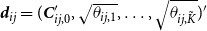 $\textbf{d}_{ij}=(\textbf{C}_{ij,0}^{\prime},\sqrt{\theta_{ij,1}},\ldots,\sqrt{\theta_{ij,\tilde{K}}})^{\prime}$
. Let
$\textbf{d}_{ij}=(\textbf{C}_{ij,0}^{\prime},\sqrt{\theta_{ij,1}},\ldots,\sqrt{\theta_{ij,\tilde{K}}})^{\prime}$
. Let
 $\bullet$
refer to conditioning on all the other parameters, latent states of the model, and the data; then the posterior distribution of
$\bullet$
refer to conditioning on all the other parameters, latent states of the model, and the data; then the posterior distribution of
 $\textbf{d}_{ij}$
is a multivariate Gaussian,
$\textbf{d}_{ij}$
is a multivariate Gaussian,
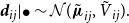 \begin{equation}\textbf{d}_{ij}|\bullet\sim\mathcal{N}({\tilde{\boldsymbol\mu}}_{ij},{\tilde{\boldsymbol V}}_{ij}).\end{equation}
The posterior moments are
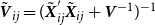 $\tilde{\textbf{V}}_{ij} = (\tilde{\textbf{X}}_{ij}^{\prime}\tilde{\textbf{X}}_{ij}+\textbf{V}^{-1})^{-1}$
and
$\tilde{\textbf{V}}_{ij} = (\tilde{\textbf{X}}_{ij}^{\prime}\tilde{\textbf{X}}_{ij}+\textbf{V}^{-1})^{-1}$
and
 $\tilde{{\boldsymbol\mu}}_{ij}=\tilde{\textbf{V}}_{ij}(\tilde{\textbf{X}}_{ij}^{\prime}\tilde{\textbf{Y}}_{ij} + \textbf{V}^{-1}{\boldsymbol\mu})$
, with prior moments
$\tilde{{\boldsymbol\mu}}_{ij}=\tilde{\textbf{V}}_{ij}(\tilde{\textbf{X}}_{ij}^{\prime}\tilde{\textbf{Y}}_{ij} + \textbf{V}^{-1}{\boldsymbol\mu})$
, with prior moments
 ${\boldsymbol\mu}=(\mu_{c1},\ldots,\mu_{c\tilde{K}},0,\ldots,0)^{\prime}$
and
${\boldsymbol\mu}=(\mu_{c1},\ldots,\mu_{c\tilde{K}},0,\ldots,0)^{\prime}$
and
 $\textbf{V}=\text{diag}\left(\lambda_c^2\times(\tau_{ci1}^2,\ldots,\tau_{ci\tilde{K}}^2),\lambda_\theta^2\times\right.$
 $\left. (\tau_{\theta i1}^2,\ldots,\tau_{\theta i\tilde{K}}^2)\right)$
. The matrix
$\left. (\tau_{\theta i1}^2,\ldots,\tau_{\theta i\tilde{K}}^2)\right)$
. The matrix
 $\tilde{\textbf{X}}_{ij}$
is of dimension
$\tilde{\textbf{X}}_{ij}$
is of dimension
 $T\times2\tilde{K}$
, with the tth row given by
$T\times2\tilde{K}$
, with the tth row given by
 $[\textbf{x}_{it}^{\prime},\tilde{\textbf{C}}_{ij,t}^{\prime}\odot\textbf{x}_{it}^{\prime}]\exp\!(-\omega_{ij,t}/2)$
,
$[\textbf{x}_{it}^{\prime},\tilde{\textbf{C}}_{ij,t}^{\prime}\odot\textbf{x}_{it}^{\prime}]\exp\!(-\omega_{ij,t}/2)$
,
 $\tilde{\textbf{Y}}_{ij}$
is
$\tilde{\textbf{Y}}_{ij}$
is
 $T\times1$
with tth element
$T\times1$
with tth element
 $\tilde{y}_{ij,t}\exp\!(-\omega_{ij,t}/2)$
. This normalization enables to draw the coefficients from standard posterior quantities for the parameters of a linear regression model with standard normal errors.
$\tilde{y}_{ij,t}\exp\!(-\omega_{ij,t}/2)$
. This normalization enables to draw the coefficients from standard posterior quantities for the parameters of a linear regression model with standard normal errors.
Factor model for the reduced form shocks
With a similar normalization based on the elements collected in
 ${\boldsymbol\Omega}_t$
, equation (1) can be used to sample the free elements of the loadings matrix
${\boldsymbol\Omega}_t$
, equation (1) can be used to sample the free elements of the loadings matrix
 $\textbf{L}$
—given the prior variances
$\textbf{L}$
—given the prior variances
 $\lambda_L^2\times(\tau_{L1}^2,\ldots,\tau_{LR}^2)$
—and the latent factors
$\lambda_L^2\times(\tau_{L1}^2,\ldots,\tau_{LR}^2)$
—and the latent factors
 $\textbf{f}_t$
conditional on each other. Note that the prior variances of the factors are determined by
$\textbf{f}_t$
conditional on each other. Note that the prior variances of the factors are determined by
 $\exp\!(h_t)\times{\boldsymbol\Sigma}$
, and posterior moments for the Bayesian linear regression model apply for sampling the factors t-by-t.
$\exp\!(h_t)\times{\boldsymbol\Sigma}$
, and posterior moments for the Bayesian linear regression model apply for sampling the factors t-by-t.
The horseshoe prior
The horseshoe (HS) prior of Carvalho et al. (Reference Carvalho, Polson and Scott2010) is used for several parts of the parameter space (the constant part of the regression coefficients, the state innovation variances and the factor loadings). Below, I present a stylized version of the prior and resulting posteriors which is universally applicable. For a generic parameter
 $b_i$
with prior mean
$b_i$
with prior mean
 $\underline{b}_i$
for
$\underline{b}_i$
for
 $i=1,\ldots,K$
, the HS prior is given by:
$i=1,\ldots,K$
, the HS prior is given by:
 \begin{equation*}b_i|c_i,d \sim \mathcal{N}(\underline{b}_i,c_i^2d^2),\quad c_i\sim\mathcal{C}^{+}(0,1),\quad d\sim\mathcal{C}^{+}(0,1).\end{equation*}
I rely on this prior in its auxiliary representation as in Makalic and Schmidt (Reference Makalic and Schmidt2015) for efficient sampling of the local (
 $c_i$
) and global (d) shrinkage parameters:
$c_i$
) and global (d) shrinkage parameters:
 \begin{equation*}c_i^2|e_i\sim\mathcal{G}^{-1}(1/2,1/e_i),\quad d^2|f\sim\mathcal{G}^{-1}(1/2,1/f), \quad e_i\sim\mathcal{G}^{-1}(1/2,1), \quad f\sim\mathcal{G}^{-1}(1/2,1).\end{equation*}
Here,
 $\mathcal{G}^{-1}$
denotes the inverse Gamma distribution. This setup yields the following conditional posterior distributions:
$\mathcal{G}^{-1}$
denotes the inverse Gamma distribution. This setup yields the following conditional posterior distributions:
 \begin{align*}c_i^2|b_i,d,e_i&\sim\mathcal{G}^{-1}\left(1,\frac{1}{e_i}+\frac{(b_i-\underline{b}_i)^2}{2d^2}\right), \quad d^2|b_i,c_i,f\sim\mathcal{G}^{-1}\left(\frac{K+1}{2},\frac{1}{f}+\sum_{i=1}^K \frac{(b_i-\underline{b}_i)^2}{2c_i^2}\right),\\e_i|c_i&\sim\mathcal{G}^{-1}\left(1,1+c_i^{-2}\right),\quad f|d\sim\mathcal{G}^{-1}\left(1,1+d^{-2}\right).\end{align*}
B: MCMC algorithm
The full MCMC algorithm cycles through the following steps:
-
1. The constant part of the coefficients and the process variances of the coefficients are simulated equation-by-equation using equation (A.1), discussed in detail in Appendix A.
-
2. For
 $\{\tilde{\textbf{C}}_{ij,t}\}_{t=1}^{T}$
, I rely on a forward-filtering backward-sampling (FFBS) algorithm (see Carter and Kohn (Reference Carter and Kohn1994); Frühwirth-Schnatter (Reference Frühwirth-Schnatter1994)). Conditional on all other parameters of the model and the constant part of the parameters, this involves Kalman filtering the states forward in time to obtain the respective conditional distributions. Subsequently, a simulation smoother is used to adjust the states based on full-sample information. For a textbook introduction, see Kim and Nelson (Reference Kim and Nelson1999).
$\{\tilde{\textbf{C}}_{ij,t}\}_{t=1}^{T}$
, I rely on a forward-filtering backward-sampling (FFBS) algorithm (see Carter and Kohn (Reference Carter and Kohn1994); Frühwirth-Schnatter (Reference Frühwirth-Schnatter1994)). Conditional on all other parameters of the model and the constant part of the parameters, this involves Kalman filtering the states forward in time to obtain the respective conditional distributions. Subsequently, a simulation smoother is used to adjust the states based on full-sample information. For a textbook introduction, see Kim and Nelson (Reference Kim and Nelson1999). -
3. Conditional on the country-specific coefficients and state innovation variances, it is straightforward to obtain a draw for the prior variances determined by the HS prior using formulae stated in Appendix A.
-
4. Simulation of
$\{\omega_{ij,t}\}_{t=1}^{T}$
is carried out using the algorithm set forth in Kastner and Frühwirth-Schnatter (Reference Kastner and Frühwirth-Schnatter2014), implemented in the R-package stochvol. The package moreover draws the innovation variances of the stochastic volatility processes. -
5. Given
$\{\textbf{f}_t\}_{t=1}^{T}$
, the factor loadings in
$\textbf{L}$
can be sampled based on the moments found in the context of a conventional linear regression model. Conditional on a draw of
$\textbf{L}$
, I obtain the corresponding HS prior variances. Moreover, the factors can be sampled conditional on
$\textbf{L}$
and
$h_t$
on a t-by-t basis. -
6. The full history for
$\{h_t\}_{t=1}^{T}$
is sampled via a random walk Metropolis–Hastings algorithm (Jacquier et al. (Reference Jacquier, Polson and Rossi2002)). This algorithm establishes conditional priors for each point in time based on the state equation which defines the joint distribution of
$h_t$
and
$h_{t-1}$
. A candidate value is proposed from
$h_t^\ast\sim\mathcal{N}(h_t,\kappa_h)$
, with
$\kappa_h$
denoting a tuning parameter (calibrated such that the acceptance rate lies around
$0.25$
). Combining the conditional prior at time t with the likelihood of the model allows for computing the acceptance probability. Conditional on
$\{h_t\}_{t=1}^{T}$
, the innovation variance
$\sigma_h^2$
can be sampled from a conventional inverse Gamma distributed posterior based on the moments found in the context of the Bayesian linear regression model.


For the empirical application, I iterate through this algorithm 12,000 times and discard the initial 2000 draws as burn-in. I consider each fourth draw of the remaining 8000 resulting in a set of 2000 draws for posterior inference. It is worth mentioning that the algorithm exhibits satisfactory convergence properties for most parts of the parameter space.
C: Country-specific VAR models
The country-specific TVP-VAR-FSVM models are defined analogously to the multi-country framework set forth in equations (1) and (2), subject to several restrictions that rule out spillovers and joint dynamics. Let
 ${\boldsymbol\epsilon}_{it}$
denote the reduced form shocks to the endogenous variables
${\boldsymbol\epsilon}_{it}$
denote the reduced form shocks to the endogenous variables
 $\textbf{y}_{it}$
. The model for country
$\textbf{y}_{it}$
. The model for country
 $i=1,\ldots,N$
is defined as:
$i=1,\ldots,N$
is defined as:
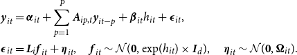 \begin{align*}\textbf{y}_{it} &= {\boldsymbol\alpha}_{it} + \sum_{p=1}^{P} \textbf{A}_{ip,t} \textbf{y}_{it-p} + {\boldsymbol\beta}_{it} h_{it} + {\boldsymbol\epsilon}_{it},\\{\boldsymbol\epsilon}_{it} &= \textbf{L}_i \textbf{f}_{it} + {\boldsymbol\eta}_{it}, \quad \textbf{f}_{it} \sim \mathcal{N}(\textbf{0},\exp\!(h_{it})\times\textbf{I}_d), \quad {\boldsymbol\eta}_{it}\sim\mathcal{N}(\textbf{0},{\boldsymbol\Omega}_{it}).\end{align*}
Different to the multi-country framework, the common uncertainty measure
 $h_{it}$
is thus defined specific to the domestic variables. Moreover, this specification rules out both static and dynamic interdependencies, since
$h_{it}$
is thus defined specific to the domestic variables. Moreover, this specification rules out both static and dynamic interdependencies, since
 $\textbf{L}_i$
only loads on a country-specific factor
$\textbf{L}_i$
only loads on a country-specific factor
 $\textbf{f}_{it}$
and there are no cross-country lagged relationships between variables (corresponding to
$\textbf{f}_{it}$
and there are no cross-country lagged relationships between variables (corresponding to
 $\textbf{B}_{iq,t} = \textbf{0}$
). I estimate these models using the same priors and sampling algorithm, with
$\textbf{B}_{iq,t} = \textbf{0}$
). I estimate these models using the same priors and sampling algorithm, with
 $P=3$
and
$P=3$
and
 $d=4$
on a country-by-country basis.
$d=4$
on a country-by-country basis.
D: Additional empirical results
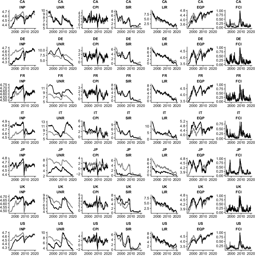
Fig. 5. Endogenous variables. Notes: Time series of the endogenous variables in black. The grey line is the cross-sectional average by variable type. Variable types in columns, countries in rows.
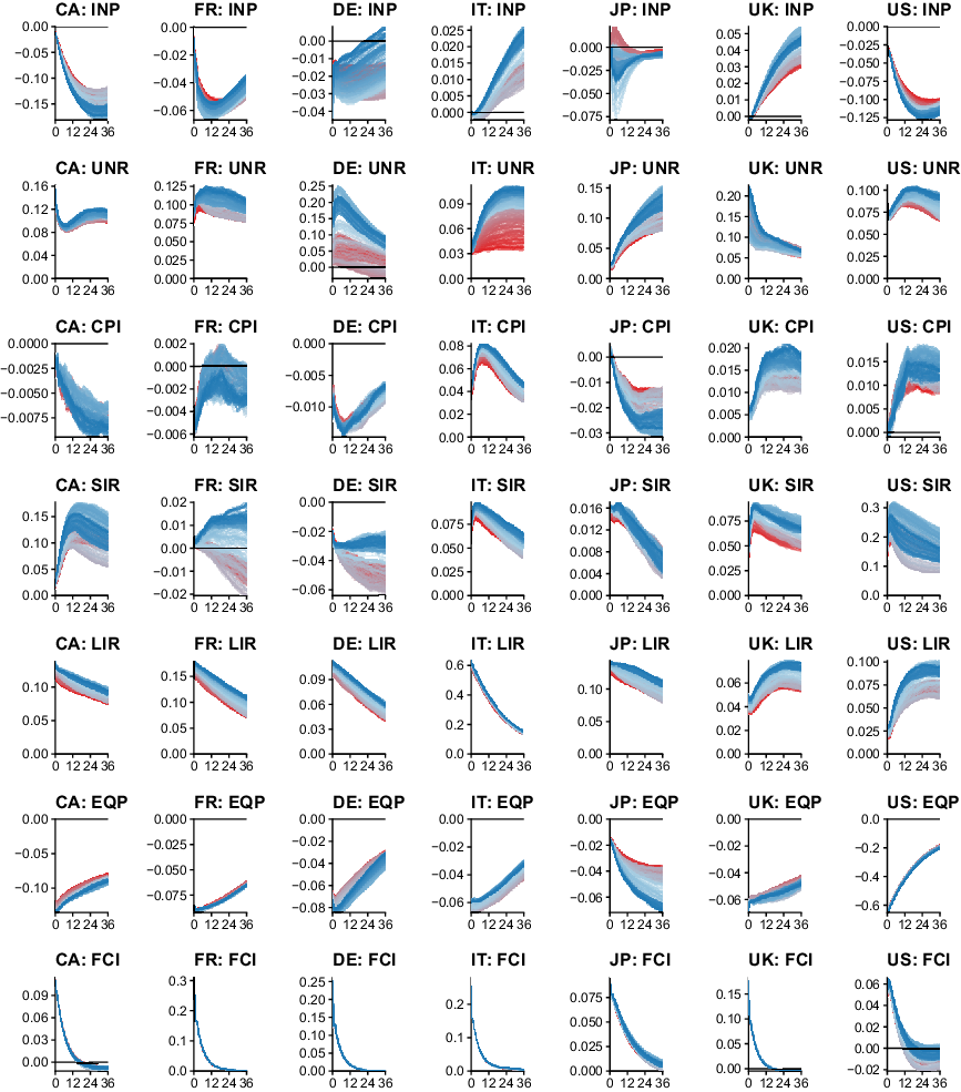
Fig. 6. Posterior median of impulse responses to an uncertainty shock over time. Notes: The lines indicate the posterior median impulse response function; they are colored with respect to time. Gradient from 1995:04 [red], 2007:08 [light blue], 2019:12 [dark blue].
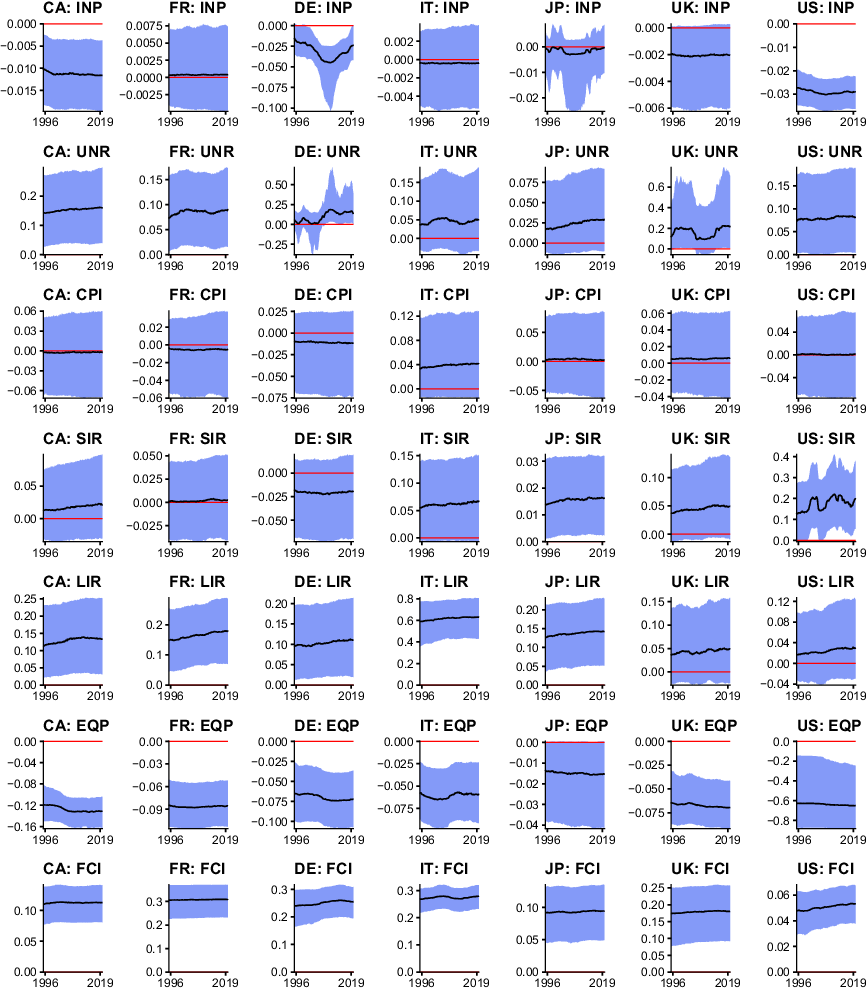
Fig. 7. Impact response to international uncertainty shocks. Notes: The solid red horizontal line marks zero, the solid black line is the posterior median estimate of the contemporaneous impact response
 ${\boldsymbol\beta}_{it}$
. The blue-shaded area covers the 50% posterior credible interval.
${\boldsymbol\beta}_{it}$
. The blue-shaded area covers the 50% posterior credible interval.
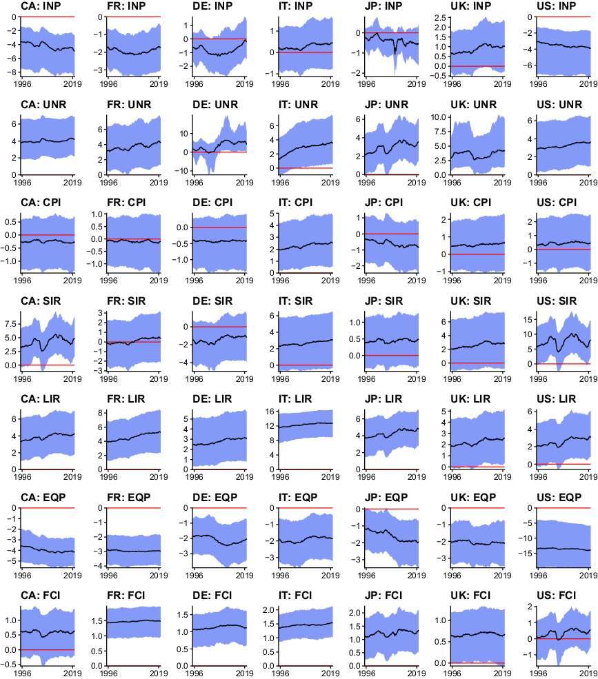
Fig. 8. Cumulative 3-year ahead response to international uncertainty shocks. Notes: The solid red horizontal line marks zero, the solid black line is the posterior median estimate of the cumulative three-year ahead response. The blue shaded area covers the 50% posterior credible interval.


 Open access