


1. Introduction
Underwater shock wave propagation in a liquid–gas medium results in many intriguing physical phenomena. Generally, the interaction of a shock wave with an individual bubble represents a conversion of acoustic energy into bubble motion or even collapse. When the shock driving is strong enough, the collapse of an initially spherical cavity can occur in a non-spherical way and thereby produce a high-speed jet, be it in a fluid (Ohl & Ikink Reference Ohl and Ikink2003), a solid (Escauriza et al. Reference Escauriza2020) or in a soft medium like gelatine (Dear, Field & Walton Reference Dear, Field and Walton1988; Swantek & Austin Reference Swantek and Austin2010; Hopfes et al. Reference Hopfes, Wang, Giglmaier and Adams2019). The piston-like motion of such a jet and its impact on the opposite bubble wall can produce further shock waves (Plesset & Chapman Reference Plesset and Chapman1971; Lauterborn & Bolle Reference Lauterborn and Bolle1975; Shima, Tomita & Takahashi Reference Shima, Tomita and Takahashi1984; Johnsen & Colonius Reference Johnsen and Colonius2009), which in turn may trigger the collapse of neighbouring bubbles. The strong energy conversion from such acoustically driven bubble collapses can be leveraged in applications such as ultrasonic cleaning (Ohl et al. Reference Ohl, Arora, Dijkink, Janve and Lohse2006a; Mason Reference Mason2016), liquid sterilisation (Abe et al. Reference Abe, Ohtani, Takayama, Nishio, Mimura and Takeda2010), bubble curtains (Bohne, Grießmann & Rolfes Reference Bohne, Grießmann and Rolfes2019; Raimbaud et al. Reference Raimbaud, Monloubou, Kerampran and Cantat2021) and ablation of kidney stones and gall stones in therapeutic shock wave lithotripsy (Sackmann et al. Reference Sackmann1988; Johnsen & Colonius Reference Johnsen and Colonius2008). Shock-induced cavitation (Ohl et al. Reference Ohl, Arora, Ikink, de Jong, Versluis, Delius and Lohse2006b; Le Gac et al. Reference Le Gac, Zwaan, van den Berg and Ohl2007) has been found to improve the permeability of cell membranes, resulting in the transfer of foreign bodies in vitro and in vivo into cells (Delius & Adams Reference Delius and Adams1999; Zhong et al. Reference Zhong, Lin, Xi, Zhu and Bhogte1999; Bekeredjian et al. Reference Bekeredjian, Bohris, Hansen, Katus, Kuecherer and Hardt2007).
A fundamental understanding of the physics behind shock–bubble interactions at the single bubble level can help to control and optimise them in applications leveraging bubble-jets on demand. A number of past studies have managed to visualise shock–bubble interactions at the millimetric (Haas & Sturtevant Reference Haas and Sturtevant1987; Layes, Jourdan & Houas Reference Layes, Jourdan and Houas2009) and even micrometric (Philipp et al. Reference Philipp, Delius, Scheffczyk, Vogel and Lauterborn1993; Kodama & Takayama Reference Kodama and Takayama1998; Ohl & Ikink Reference Ohl and Ikink2003; Wolfrum et al. Reference Wolfrum, Kurz, Mettin and Lauterborn2003; Abe et al. Reference Abe, Wang, Shioda and Maeno2015) scale despite the experimental challenges imposed by their small spatial and temporal scales. These experiments included a variety of underwater shock wave generation methods, such as lithotripters (Philipp et al. Reference Philipp, Delius, Scheffczyk, Vogel and Lauterborn1993), lasers (Wolfrum et al. Reference Wolfrum, Kurz, Mettin and Lauterborn2003) and underwater explosions (Kodama & Takayama Reference Kodama and Takayama1998). They have confirmed, for instance, that the radial bubble dynamics are well predicted by numerically solving the Keller–Miksis equation (Keller & Miksis Reference Keller and Miksis1980; Philipp et al. Reference Philipp, Delius, Scheffczyk, Vogel and Lauterborn1993; Wolfrum et al. Reference Wolfrum, Kurz, Mettin and Lauterborn2003; Abe et al. Reference Abe, Wang, Shioda and Maeno2015). The formation of a thin liquid jet in the direction of shock propagation has been imaged and its average velocity found to be in the range 20– $200\ {\rm ms}^{-1}$ (Philipp et al. Reference Philipp, Delius, Scheffczyk, Vogel and Lauterborn1993; Ohl & Ikink Reference Ohl and Ikink2003). The damage potential of such jets has been demonstrated through, for example, characterisation of their penetration depth into gelatine (Kodama & Takayama Reference Kodama and Takayama1998). Numerical studies on shock–bubble interactions using finite volume method (Ding & Gracewski Reference Ding and Gracewski1996), front-tracking method (Betney et al. Reference Betney, Tully, Hawker and Ventikos2015), boundary integral method (Calvisi et al. Reference Calvisi, Lindau, Blake and Szeri2007; Klaseboer et al. Reference Klaseboer, Fong, Turangan, Khoo, Szeri, Calvisi, Sankin and Zhong2007), a high-order accurate shock and interface-capturing scheme (Johnsen & Colonius Reference Johnsen and Colonius2008, Reference Johnsen and Colonius2009) and the improved ghost fluid method (Kobayashi, Kodama & Takahira Reference Kobayashi, Kodama and Takahira2011) have been able to compute bubble shapes and key parameters such as the jet velocity, kinetic energy and bubble centroid translations to varying accuracy. Nonetheless, many of these valuable numerical results still lack experimental benchmarks which, in turn, has prevented the development of reliable scaling laws to describe shock-driven bubble dynamics in a simpler framework to, for example, reduce the computational cost for modelling complex multibubble systems. Furthermore, much of the modelling efforts have thus far focused on effective shock widths much larger than the bubble size with inconclusive knowledge on waveform effects. The present study aims to fill these knowledge gaps by reporting on experiments of unprecedented detail on impulsive shock waves, i.e. shock waves with finite thickness, interacting with bubbles and by proposing scaling laws for the key parameters describing the ensuing bubble collapse.
2. Methods
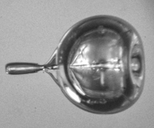
In the experiment (figure 1a), two different techniques are used to produce bubbles at distinct size ranges in a test chamber filled with deionised water. Air bubbles with initial radii of  $r_{0} = 80\unicode{x2013}500 \ \mathrm {\mu }{\rm m}$ (figure 1b) are generated using a flow-focusing microfluidic device following the concept detailed by Benson, Stone & Prud'homme (Reference Benson, Stone and Prud'homme2013), while smaller bubbles are generated through electrolysis with radii of $r_0 = 10\unicode{x2013}50 \ \mathrm {\mu }{\rm m}$ and a hydrogen core (figure 1c). The bubbles are let to rise freely through buoyancy.

Figure 1. (a) Schematic of the experimental set-up. (b) Image sequence of an air bubble interacting with a shock wave of peak pressure  $p_{max} = 42.68 \ {\rm MPa}$ and temporal width $\delta = 32.66 \ {\rm ns}$ (adapted from Bokman & Supponen (Reference Bokman and Supponen2021)). The dimensionless time, $t/(r_{0}\sqrt {\rho /p_{b,0}})$, is displayed in each frame and is zero on the frame where the shock front has crossed the bubble centre. The shock front has been graphically highlighted for visual clarity. (c) Image sequence of a hydrogen bubble interacting with a shock wave of $p_{max} = 25.35 \ {\rm MPa}$ and $\delta = 37.55 \ {\rm ns}$. See supplementary movies available at https://doi.org/10.1017/jfm.2023.514.
The underwater shock wave is produced through optical breakdown by focusing an expanded high-power, pulsed Nd:YAG laser beam (Lumibird Quantel Q-smart, 532 nm, 6 ns, 220 mJ) in the water 6 mm away from the bubble stream. The peak pressure of the spherically propagating shock wave,  $p_{max}$, can be varied by tuning the laser power and the resulting shock wave energy (0.05–9 mJ). The temporal pressure profile of the shock wave, $p_{a}$, (figure 2) is recorded by a piezoelectric needle hydrophone (Precision Acoustics, 75 $\mathrm {\mu }$m sensor) located $41.60$ mm away from the source, and shows a finite width and decaying tail. The total shock wave duration, $t_{I}$, which represents the excess pressure contributing to the bubble collapse, is taken from the first moment at which the pressure exceeds 10 % of $p_{max}$ until it once again reaches the average noise level. The peak pressure measured at the hydrophone varies between $0.34$– $3.42$ MPa, while the measured temporal shock width at half-maximum remains approximately constant when varying the laser power, with an average of $\delta = 52.43 \pm 5.99$ ns. The rise time of the recorded pressure signals is found to be approximately 14 ns, and is measured from 10 % to 90 % of the shock wave's peak pressure.

Figure 2. Hydrophone recording of the pressure waveform of a laser-induced underwater shock wave with respect to time, normalised to the ambient pressure  $p_{0}$ and the temporal full-width at half-maximum $\delta$, respectively. The red curve is an idealised shock wave pressure profile computed with the Friedlander model for $b = 10$.
High-speed shadowgraphy using an ultra-high-speed CMOS camera (Shimadzu HPV-X2) equipped with a long-distance microscope objective (Keyence, VH-Z50L) and a collimated halogen fibre optic as backlight illumination is used to visualise the bubble dynamics. The imaging frame rate is set to 0.5–10 Mfps depending on the bubble size. For jetting bubbles larger than  $100 \ \mathrm {\mu }{\rm m}$, a front illumination with high-voltage xenon flashlamps (Cordin Model 605) allows, on some occasions, the visualisation of the jets along their entire trajectory inside the bubble, as seen in figure 1(b). In all cases, the spherically propagating shock wave can be visualised. The shock is assumed to interact with the bubbles similarly to a plane wave due to the small bubble size relative to the shock radius. This assumption, however, approaches its limit for large bubbles as seen in figure 1(b), in which the shock wave shows an appreciable curvature relative to the bubble size. The recorded water temperature remains between $20$–
$20$– $22\,^\circ$C and the ambient pressure between $p_{0}=96$– $104 \ {\rm kPa}$ throughout the experiments.
3. Results and discussion
3.1. Shock wave pressure profile
Due to the risk of hydrophone damage close to the shock wave source, the shock wave pressure profile cannot be experimentally quantified in the region of interest, located 6 mm away from its origin, and is instead recorded in the far field, at a distance of 41.60 mm. However, the peak pressure and width of the shock wave are expected to change during its propagation in water due to nonlinear dissipation caused by inelastic heating and gaseous contaminants as well as spherical spreading. In fact, Vogel et al. (Reference Vogel, Busch and Parlitz1996) have reported both experimentally and numerically an exponential relation between the shock wave peak pressure and the distance over which it propagates. Generally, the peak pressure is found to decay slower in the far field (millimetres) than in the near field (micrometres). The values of the exponential relation range from  $p_{max} \propto x^{-2.5}$ to $p_{max} \propto x^{-1.02}$, depending on the radial distance, $x$, where $x = 0$ at the origin of the shock wave. Additionally, the nonlinearity of shock wave propagation increases the shock wave peak duration as it propagates far away from its origin. These findings suggest that the exponential relation between the peak pressure and shock width with respect to the propagation distance, $x$, allows for the estimation of the shock wave's peak pressure and full-width at half-maximum at the bubble location from the hydrophone recordings, where $x$ is the distance between the bubble and the hydrophone.
Here, the exponent describing the decay of the peak pressure and the widening of the shock width with respect to the distance are estimated through hydrodynamic simulations using the open-source code ECOGEN (Schmidmayer et al. Reference Schmidmayer, Petitpas, Le Martelot and Daniel2020), which has been extensively validated for compressible flows. The shock wave is modelled as it travels between the bubble and the hydrophone, and where  $x = 0$ at the origin of the shock wave. The initial conditions of the spherical shock wave are set to match the experimental pressure profile at the bubble-to-hydrophone distance. The peak pressure and full-width at half-maximum of the shock are, respectively, found to scale with $x^{-1.4}$ and $x^{0.2}$ (figure 3) between the bubble and hydrophone, which are in good agreement with previously reported measurements (Vogel et al. Reference Vogel, Busch and Parlitz1996). The use of these exponents to scale the recorded pressure waveform to the true pressure acting on the bubble can be assessed by two distinct methods.

Figure 3. Numerically computed evolution of the shock wave peak pressure,  $p_{max}$, and the spatial half-width at half-maximum, $\delta _{{x}}$, normalised to their initial values $p(0)$ and $\delta _{{x}}(0)$, with the distance, $x$, travelled by the shock wave, respectively. The solid and dashed lines display their power law fits.
The first method consists in assessing experimentally the exponential decay and spreading of the peak pressure and shock width, respectively. The pressure profile of the same shock wave is recorded using two hydrophones located at different distances from the shock wave's emission centre, and far enough to avoid hydrophone damage. Here, the hydrophones are located at a distance of  $17$ mm and $64$ mm (Hyd. 1 and Hyd. 2 in figure 4a) from the shock wave's origin, and as close as possible to a shared axis, while making sure that Hyd. 1 does not affect the measurement of Hyd. 2. The corresponding raw pressure recordings $(M)$ are displayed in figure 4(a) and show an appreciable dissipation of the shock wave pressure profile recorded by the second hydrophone. The total shock wave duration, $t_{I}$ is highlighted in dark red for Hyd. 1 and light red for Hyd. 2. ECOGEN simulations estimate the peak pressure to decay as $x^{-1.2}$ and the full-width at half-maximum to spread as $x^{0.1}$ on the distance between the two hydrophones. In figure 4(b), the pressure signal recorded by Hyd. 2 (light red) is scaled $(S)$ both in height and width, to the location of Hyd. 1 (dark red), using the exponential relations provided by ECOGEN in the form $p_{max,1} = p_{max,2}(t_{0,1}/t_{0,2})^{-1.2}$ and $\delta _{1} = \delta _{2}(t_{0,1}/t_{0,2})^{0.1}$, where $t_{0,i}$ is the moment (after shock initiation at $t=0$) at which the shock wave reaches the hydrophone and $i = 1,2$ denotes either Hyd. 1 or Hyd. 2.

Figure 4. (a) Hydrophone measurement  $(M)$ of the pressure waveform of a laser-induced underwater shock wave with respect to time, normalised to the ambient pressure $p_{0}$ and the temporal full-width at half-maximum $\delta$, respectively. The shock wave pressure is measured by two hydrophones located at different distances $x$, from the source and $t_0$ is the time it takes for the shock to reach the sensor. The peak pressure, $p_{max}$, full-width at half-maximum, $\delta$, total over-pressure duration, $t_{I}$, pressure impulse, $j$, and distance to the shock wave source, $x$, are given for both recordings. (b) Comparison of the pressure waveform recorded by Hyd. 1 and the one recorded by Hyd. 2, when scaled $({S})$ to the location of Hyd. 1. The scaled peak pressure, $p_{max}$, full-width at half-maximum, $\delta$ and pressure impulse, $j$ are also provided. The pressure is filtered using a Savitzky–Golay filter (Press & Teukolsky Reference Press and Teukolsky1990) of polynomial-order three and window length of 50 points. The vertical lines indicate the moment the shock wave reaches the mean pressure noise level, representing the end of the shock wave.
The shock wave peak recorded by Hyd. 2 and scaled to the location of Hyd. 1 is in very good agreement with the one recorded by Hyd. 1. The error on the peak pressure and full-width at half-maximum are within 5 % and 6 %, respectively. However, the pressure fluctuations present in the shock wave tail do not match well despite being in the same order of magnitude. The second and third pressure peaks recorded by Hyd. 1 show a time shift with respect to those recorded by Hyd. 2. This occurs because the shock wave duration,  $t_{I}$, becomes shorter as it travels (Shi et al. Reference Shi, Li, Hu, Li, Wu, Chen and Qiu2022) due to nonlinear dissipation. The total contribution of the shock wave, represented as the magnitude of the pressure impulse (Tomita & Shima Reference Tomita and Shima1986; Tagawa et al. Reference Tagawa, Yamamoto, Hayasaka and Kameda2016)
 \begin{equation} j = \int_{t_0}^{t_0+t_{I}} p_{a}(t) \, \mathrm{d}t,\end{equation}
indicates that the scaled pressure recording of Hyd. 2 underestimates the magnitude of the pressure impulse recorded by Hyd. 1 by 14 %. Therefore, despite the very good agreement between the original and scaled shock wave peaks, the nonlinear dissipation of the shock wave tail fluctuations prevents a precise recovery of the shock wave profile measured by Hyd. 1 solely from the measurements of Hyd. 2 and exponential scaling relations. This remains a source of uncertainty in the present work.
The uncertainty on the scaled pressure waveform at the bubble location can be further quantified using spherical cavitation bubble theory as a second method. Indeed, previous studies have demonstrated the Keller–Miksis (Keller & Miksis Reference Keller and Miksis1980) equation to describe well experimentally visualised shock-driven radial bubble dynamics even upon strong bubble deformation (Philipp et al. Reference Philipp, Delius, Scheffczyk, Vogel and Lauterborn1993; Wolfrum et al. Reference Wolfrum, Kurz, Mettin and Lauterborn2003; Abe et al. Reference Abe, Wang, Shioda and Maeno2015), especially when the shock wave's pressure is measured at the bubble location with a fibre-optic hydrophone. Here, the simpler Rayleigh (Rayleigh Reference Rayleigh1917) and Rayleigh–Plesset (Plesset Reference Plesset1949) equations are also briefly shown and their limitations commented. The Rayleigh–Plesset equation is often used to model the radial dynamics of a spherical gas bubble interacting with external pressure driving,  $p_{a}(t)$,
 \begin{equation} \rho ( r\ddot{r} + \tfrac{3}{2}\dot{r}^{2} ) = p_{b} - p , \end{equation}
where  $r$ is the bubble radius, $\dot {r}$, $\ddot {r}$ represent the interfacial velocity and acceleration, respectively, and $\rho$ is the liquid density. The pressure on the liquid side of the bubble's interface is expressed as $p_{b} = p_{b,0}(r_{0}/r )^{3\kappa } - 2\gamma /r - 4\mu \dot {r}/r$, where the bubble gas contents are modelled through an adiabatic formulation with $p_{b,0} = p_{0} + 2\gamma /r_{0}$ being the initial pressure inside the bubble, $\kappa$ the polytropic exponent of the gas, $\gamma$ the surface tension and $\mu$ the dynamic viscosity. The pressure inside the liquid is $p(t) = p_{a}(t) + p_0$. The Rayleigh equation (Rayleigh Reference Rayleigh1917) is the simpler version of the Rayleigh–Plesset equation, where gas compression, viscosity and surface tension are neglected ( $p_{b}=p_{0}$). The Rayleigh and Rayleigh–Plesset equations (3.2) do not account for liquid compressibility, which can potentially be relevant despite the relatively low Mach numbers associated with the shock–bubble interactions (Tian et al. Reference Tian, Liu, Zhang and Tao2020; Li et al. Reference Li, Saade, van der Meer and Lohse2021) in this work ( $M_{a} < 0.2$). To account for liquid compressibility, (3.2) can be extended to the Keller–Miksis equation (Keller & Miksis Reference Keller and Miksis1980),
 \begin{equation} \left(1 - \frac{\dot{r}}{c_{0}} \right) r\ddot{r} + \frac{3}{2}\left(1 - \frac{\dot{r}}{3c_{0}} \right)\dot{r}^{2} = \left(1 + \frac{\dot{r}}{c_{0}} \right)\frac{p_{b} - p }{\rho} + \frac{r}{\rho c_{0}}\frac{\mathrm{d}p_{b}}{\mathrm{d}t}, \end{equation}
where  $c_0$ is the speed of sound in the liquid. Both (3.2) and (3.3) are numerically solved using a Runge–Kutta fourth-order method.
Figure 5(a) displays two image sequences of a bubble interacting with a shock wave of different peak pressure along with their corresponding radius-time-curves, shown in figure 5(b). Small bubbles, both of approximately  $r_0 = 30\ \mathrm {\mu }{\rm m}$, are chosen here for their short dynamics with respect to the shock wave duration, where the pressure fluctuations in the shock wave tail have a minor effect.

Figure 5. (a) Image sequence of hydrogen bubbles interacting with a shock wave of (1)  $p_{max} = 32.71 \ {\rm MPa}$ and $\delta = 37.77 \ {\rm ns}$ and (2) $p_{max} = 13.66 \ {\rm MPa}$ and $\delta = 37.92 \ {\rm ns}$. See supplementary movies. The dimensionless time, $t/(r_0 \sqrt {\rho /p_{b,0}})$, is displayed in each frame and is zero on the frame where the shock front has crossed the bubble centre. The shock front has been graphically highlighted for visual clarity. (b) Radius-time-curves and pressure waveform corresponding to both image sequences. The experimental collapse times are (1) $\tau _{c} = 0.25\ \mathrm {\mu }{\rm m}$ and (2) $\tau _{c} = 0.75\ \mathrm {\mu }{\rm m}$. The solution to the Rayleigh equation (. . . . . .), Rayleigh–Plesset (- - - - - -) and Keller–Miksis (——–) equations are displayed. The red shaded area shows the uncertainty on the bubble dynamics, based on the sensor limitation and scaling used in this work. The pressure driving is taken from scaled hydrophone recordings filtered with a Savitzky–Golay filter (Press & Teukolsky Reference Press and Teukolsky1990) of polynomial-order three and window length of 50 points.
The first case (1) shows an appreciable nonlinear collapse followed by a high-speed liquid jet travelling in the shock wave's direction. The tip of the jet can, on some occasion, overcome surface tension and entrain some gas when breaching the distal side of the bubble (Ohl & Ikink Reference Ohl and Ikink2003). Such a small gas ejecta, which has separated from the main bubble, is highlighted on the fifth frame. The second case (2) shows a weaker oscillation where the proximal side of the bubble is flattened by the shock wave, and no visible liquid jet is produced. Figure 5(b) compares the recorded radius-time-curves with spherical bubble theory. Results from the Keller–Miksis equation are indicated by full red lines, while the red shaded region represents the uncertainty on the bubble dynamics caused by the pressure waveform. The shaded region is estimated from the 20 % uncertainty on the hydrophone pressure recordings, and the 14 % uncertainty induced by the shift in the peaks of the shock wave tail fluctuations. Results from the Rayleigh and Rayleigh–Plesset equations are shown in black dotted and dashed lines, respectively. The first case of a  $r_0 = 27 \ \mathrm{\mu }{\rm m}$ bubble interacting with a shock wave of $p_{max} = 32.71 \ {\rm MPa}$ and $\delta = 37.77 \ {\rm ns}$ agrees quite well with results from the Keller–Miksis equation. In this case, the very short duration of the bubble collapse with respect to the shock wave duration makes the main shock wave peak the major contributor to the bubble collapse. The shift of the tail fluctuations, presented in figure 4(b), causes the model to predict a slightly earlier collapse. The Rayleigh and Rayleigh–Plesset equations indicate almost the same collapse time, $\tau _{c}$, defined as the time between the instant of the shock wave acting on the bubble to that of the bubble reaching its minimum radius. This suggests that for a strong collapse the polytropic compression of the non-condensable gas, surface tension and viscosity do not affect the collapse time considerably and that the dynamics are inertially driven. Both equations underestimate the collapse time obtained from the Keller–Miksis equation by approximately 7 %, which is caused by neglecting compressible effects. In the second case (2), the bubble has an initial radius of $r_0 = 30 \ \mathrm{\mu }{\rm m}$ and interacts with a weaker shock wave of $p_{max} = 13.66 \ {\rm MPa}$ and $\delta = 37.92 \ {\rm ns}$. The dynamics are slower than in the first case and the uncertainty on the shock wave tail fluctuations has a stronger effect than in the previous case. Here again, the shift of the tail fluctuations accelerate the bubble collapse in the model. As the polytropic compression plays a major role here, the estimation of the collapse time by the Rayleigh equation, which considers the bubble gas pressure to remain constant, is found to be almost 30 % shorter than the actual collapse. However, results from the Rayleigh–Plesset and Keller–Miksis equations are similar, indicating almost negligible compressible effects. In both cases, the bubble dynamics are well captured by the Keller–Miksis equation within the uncertainty of the pressure measurement. For a strong shock wave, the bubble dynamics are mainly inertially driven and the Rayleigh equation estimates the collapse time almost as well as the Rayleigh–Plesset equation, but both are slightly off due to non-negligible compressible effects. In the case of a weaker bubble oscillation, the Rayleigh equation cannot be used, but discrepancies between the Rayleigh–Plesset and Keller–Miksis equations are almost negligible.
The two methods presented in this section to evaluate the quality of the scaling of the recorded pressure to the bubble location provide a reasonable estimate of the actual shock wave peak acting on the bubble. However, uncertainty on the shock wave tail fluctuations and total over-pressure duration remains. Due to the experimental limitations and complexity of the experiment, the uncertainty is deemed acceptable when confirming the scaling of different quantities such as the collapse time or liquid jet speed, within the limits of the pressure measurements. Applying this scaling to the hydrophone measurement yields  $p_{max} = 7.35$– $72.66 \ {\rm MPa}$ and $\delta = 32.92 \pm 4.02 \ {\rm ns}$ at the location of the bubbles. The propagation speed and maximum particle velocity of these shock waves is estimated at $u_{s} = 1.52 \pm 0.02\ {\rm km}\ {\rm s}^{-1}$ and $u_{p} = 4.84-43.85\ {\rm m}\ {\rm s}^{-1}$ with the Rankine–Hugoniot jump relations. The propagation speed is verified experimentally and in agreement with previous studies (Vogel, Busch & Parlitz Reference Vogel, Busch and Parlitz1996; Noack & Vogel Reference Noack and Vogel1998) when the probe is located millimetres away from the shock source. The particle velocity is expected to decrease exponentially with the shock pressure, and to have little effect on bubble dynamics. The resulting computed spatial half-width at half-maximum at the bubble location is $\delta _{{x}}= u_{s}\delta = 50.04 \pm 6.11\ \mathrm {\mu }$m.
3.2. Collapse time
Under some assumptions, it is possible to derive an analytical expression for the collapse time of a shock-driven bubble as a simpler alternative to numerically solving the Rayleigh–Plesset or Keller–Miksis equations. This can be achieved by performing a similar derivation to that of the collapse time for vapour cavities, known as the Rayleigh collapse time. The Rayleigh collapse time is computed by integrating the Rayleigh equation and reads  $\tau _{c} = 0.915r_{0}({\rho }/{\rm \Delta} p)^{1/2}$. Here, 0.915 is the universal Rayleigh factor and the driving pressure difference reads ${\rm \Delta} p = p_{0} - p_{v}$, where $p_{v}$ is the saturated vapour pressure. The Rayleigh collapse time neglects surface tension, viscosity, non-constant pressure inside the bubble, liquid compressibility and deviations from spherical symmetry. Despite these limitations, numerical studies have shown that the collapse time of gas bubbles that are initially at equilibrium with the surroundings and driven by a travelling shock wave can be approximated in a similar way by expressing ${\rm \Delta} p = p_{max}-p_{0}$, despite the strong deformation of bubbles during shock-induced collapses (Johnsen & Colonius Reference Johnsen and Colonius2009; Kapahi, Hsiao & Chahine Reference Kapahi, Hsiao and Chahine2015). The shock wave is modelled as a step change in pressure of constant amplitude $p_{max}$ with zero rise time and infinite width. The variation in bubble pressure can be neglected and the pressure set to a constant $p_{0}$. Only a small delay to the collapse time attributed to the duration of the shock propagating along the full width of the bubble has been found (Johnsen & Colonius Reference Johnsen and Colonius2009). The validity of the Rayleigh collapse time, despite neglecting viscosity, gas content and surface tension effects, is explained by the clear domination of inertial effects for sufficiently high ${\rm \Delta} p$.
However, underwater shock waves typically have a decaying pressure profile of short and finite duration  $t_{I}$ as indicated in figure 2. In some cases, the shock driving can occur within a time scale significantly shorter than the bubble collapse time, i.e. $t_{I} \ll \tau _{c}$. Such a finite-width shock, hereinafter referred to as impulsive shock wave, is known to prolong a bubble's collapse time (Johnsen & Colonius Reference Johnsen and Colonius2008) with respect to the Rayleigh collapse due to the shorter duration of the applied pressure. Nonetheless, to the best of the authors’ knowledge, an exact scaling of the collapse time with respect to the pressure driving parameters, such as the amplitude and width of an impulsive shock wave, is yet to be described. The Keller–Miksis equation's good prediction of shock-induced bubble dynamics is herein leveraged to offer such insights. In water, the main variables influencing the dynamics of a shock-driven bubble collapse are the bubble's initial radius, $r_0$, the ambient pressure, $p_0$ and the shock wave's form, which can be described in both amplitude and width by the peak pressure, $p_{max}$, and full-width at half-maximum, $\delta$. A parametric investigation of the collapse time is displayed in figure 6. The Keller–Miksis equation is numerically solved and the collapse time extracted by taking the instant at which the bubble first expands. In this parameter space investigation, the exponentially decaying pressure profile is modelled by the modified Friedlander equation from blast wave theory (Dewey Reference Dewey2018) as $p_{a}(t) = p_{max}(1 - t/t_{I})\exp (-bt/t_{I})$, indicated by the red line in figure 2. The exponential decay of the pressure wave is described by a parameter $b = 10$, which is determined by fitting to experiments and kept constant for the shock waves investigated in the present work. The use of such an ideal pressure waveform is chosen to conduct an uncertainty-free formal analysis, which is later contrasted to experiments.

Figure 6. Parameter space investigation of the main variables influencing the collapse time,  $\tau _{c}$, using the Keller–Miksis equation and an ideal Friedlander-type shock wave profile. The shock wave peak pressure, $p_{max}$, temporal shock width, $\delta$ and initial bubble radius, $r_0$, are varied. (a) Logarithmic representation of the collapse time versus the shock peak pressure. (b) Normalisation of the collapse time to the characteristic bubble time, $r_{0}\sqrt {\rho / p_{b,0}}$ and shock wave peak pressure to the bubble pressure, $p_{b,0}$. (c) Normalisation of the collapse time to the characteristic bubble time, $r_{0}\sqrt {\rho / p_{b,0}}$ and shock wave impulse, $J$, to the characteristic bubble momentum, $r_{0}^{3}\sqrt {p_{b,0} \rho }$. The slope of the different scalings are highlighted by black dashed lines in the normalised representations.
Three bubble sizes,  $r_0 = 25,100$ and 500 $\mathrm{\mu }$m, are selected, which reflect the experimental radii encountered in this work. The shock wave amplitude covers a large range of pressures, ranging from $p_{max} = 0.2 \ {\rm MPa}$ to $p_{max} = 200 \ {\rm GPa}$. Two values are selected for the shock wave full-width at half-maximum; $\delta = 20 \ {\rm ns}$, which is in the same order of magnitude as the values recorded in the present experiments; and a larger one, $\delta = 2 \ \mathrm {\mu }{\rm s}$, which effectively acts as a shock of infinite duration for very short collapse times with respect to the over-pressure duration ( $\tau _{c} \ll t_{I}$).
The collapse time displayed in figure 6(a) decreases, unsurprisingly, with the bubble size and as the peak pressure and full-width at half-maximum increase. Three different regimes, where the collapse time exponentially scales with the pressure, are indicated by the slopes in the logarithmic representations of figure 6. When looking at the specific case of a 100  $\mathrm {\mu }{\rm m}$ bubble interacting with a shock wave of $\delta = 20$ ns, one notices, as the peak pressure increases, a first regime where the collapse time is independent from the peak pressure (slope is 0), followed by an intermediate phase where the slope is $-1$ and, at higher pressures, by a final regime in which the slope is $-1/2$. These scalings are explained in figure 6(b) upon appropriate normalisation of the collapse time to the gas bubble's characteristic time $r_{0}\sqrt {\rho /p_{b,0}}$ as well as the shock wave peak pressure to the to the bubble pressure, $p_{b,0}$. By doing so, all curves converge to the same value for the low peak pressures of the first regime. This is because a weak shock wave drives a bubble into linear, small-amplitude oscillations at the bubble's natural frequency, also known as Minnaert frequency (Minnaert Reference Minnaert1933), which is excited by the broad frequency content of an impulsive shock wave (Ohl Reference Ohl2002). Despite no real collapse taking place, a Minnaert collapse time for such linear behaviour is defined here as the quarter of the oscillation period, corresponding to the minimum of the oscillation amplitude, which can be expressed as $\tau _{c} = ({\rm \pi} /\sqrt {12\kappa })r_{0}\sqrt {\rho /p_{b,0}}$ and is the exact solution to which the collapse time converges at low peak pressures. It is expected that the dimensionless collapse time of shock-induced bubbles for small impulses is bounded by ${\rm \pi} /\sqrt {12\kappa } = 0.77$ according to the Minnaert frequency for $\kappa = 1.4$, which has been broadly adopted for air and hydrogen alike.
Figure 6(b) shows that, beyond the linear oscillation regime, the collapse time eventually scales with the peak pressure as  $\tau _{c} \propto (p_{max}/p_{b,0} -1)^{-1/2}$. This regime occurs when the bubble collapse time is much smaller than the shock wave duration ( $\tau _{c} \ll t_{I}$), which leads to the bubble effectively feeling the shock wave as a pressure wave of infinite duration. A larger temporal full-width at half-maximum with respect to the bubble collapse time or a large peak pressure which shortens the bubble collapse are necessary for this regime to take place. In fact, this scaling corresponds to the Rayleigh collapse, previously reported by Johnsen & Colonius (Reference Johnsen and Colonius2009), where bubbles interact with a shock wave modelled as a step increase in pressure of infinite duration. Therefore, the exact solution to the collapse time upon which all curves collapse for large peak pressures in figure 6(b) is $\tau _{c} = 0.915\sqrt {\rho / (p_{max} - p_{b,0})}$. The values of the collapse time that are higher than the Rayleigh solution (e.g. $r_0 = 500\ \mathrm {\mu }$m and $\delta = 20$ ns) are caused by a narrower temporal shock width with respect to the collapse time, as reported by Johnsen & Colonius (Reference Johnsen and Colonius2008).
If the shock wave duration is much shorter than the bubble dynamics, impulse theory explains the scaling of the collapse time as  $\tau _{c} \propto (p_{max}/p_{b,0})^{-1}$, which is highlighted in figure 6(b). Assuming that the bubble is initially at rest and that its radius does not change during the application of the shock-induced force on the bubble (and therefore $p_{b}=p_{b,0}$ during this time), which is confirmed experimentally for $t_{I} \ll \tau _{c}$, the magnitude of the pressure impulse (Tomita & Shima Reference Tomita and Shima1986; Tagawa et al. Reference Tagawa, Yamamoto, Hayasaka and Kameda2016) applied by the shock wave on the bubble can be computed by integrating equation (3.2) with respect to time over the shock wave duration,
 \begin{equation} j = \rho r_0 [\dot{r}(t_{I}) - \dot{r}(0) ]= \int_{0}^{t_{I}} p(t) - p_{b,0} \, \mathrm{d}t, \end{equation}
where  $p(t) = p_{a}(t) + p_0$ and $p_{a}(t)$ is the time-varying acoustic pressure of the shock waveform. The integration by parts of $3\dot {r}^2 /2$ of (3.2) yields zero. The bubble is assumed to be initially at rest and its interface velocity to impulsively jump to the finite initial velocity of $\dot {r}(t_{I}) = \dot {r}_0$. Integrating the pressure impulse, $j$, over the surface of the bubble (assuming spherical symmetry) yields
 \begin{equation} J = 4 {\rm \pi}r_{0}^{3} \rho \dot{r}_{0} = 4 {\rm \pi}r_{0}^{2}\int_{0}^{t_{I}} p(t) - p_{b,0} \, \mathrm{d}t. \end{equation}
The impulse  $J$ is analogous to the Kelvin impulse, which has been widely used to describe the deformation of collapsing vapour bubbles and corresponds to the effective impulsive force due to pressure field asymmetries caused by neighbouring boundaries, gravity or sound waves, and yielding a translational flow in the form of a jet (Blake Reference Blake1988; Best & Kucera Reference Best and Kucera1992; Brujan et al. Reference Brujan, Nahen, Schmidt and Vogel2001; Brujan, Pearson & Blake Reference Brujan, Pearson and Blake2005; Wang & Manmi Reference Wang and Manmi2014; Supponen et al. Reference Supponen, Obreschkow, Tinguely, Kobel, Dorsaz and Farhat2016). The main difference between the Kelvin impulse and $J$ is that here, $J$ is the real impulse provided by the shock wave, which drives the collapse and, contrary to the Kelvin impulse, remains finite even for spherical bubble collapses.
By expressing the pressure impulse from the Rayleigh equation, the speed of the bubble's interface right after the passage of the impulsive force can be written as a function of the pressure impulse from (3.4), as  $\dot {r}_{0} = -(\rho r_{0})^{-1}\int _{0}^{t_{I}} p(t) - p_{b,0} \, \mathrm {d}t$. As for the Rayleigh collapse time, an analytical model for the impulsive collapse time is obtained by integrating twice the Rayleigh equation while neglecting the pressure variation inside the bubble. The omission of the bubble gas pressure variation in the analysis implies that after the shock passage the bubble is at equilibrium with the surrounding pressure but has a finite initial interface velocity $\dot {r}_{0}$ driving the overall process, thus yielding the impulsive collapse time as a function of the measured waveform,
 \begin{equation} \tau_{c} = \frac{2 \rho r_{0}^{2}}{5} \left(\int_{0}^{t_{I}} p(t) - p_{b,0} \, \mathrm{d}t \right)^{{-}1}. \end{equation}
Upon normalisation to the characteristic time of the bubble,  $r_{0}\sqrt {\rho /p_{b,0}}$, and using the impulse applied to the bubble, $J$ (see (3.5)) normalised to the characteristic momentum of the bubble $r_{0}^{3}\sqrt {p_{b,0}\rho }$, the collapse time in (3.6) can be rewritten as
 \begin{equation} \frac{\tau_{c}}{r_{0}\sqrt{\rho/p_{b,0}}} = \frac{8 {\rm \pi}}{5} \left(\frac{J}{r_{0}^{3}\sqrt{p_{b,0}\rho }} \right)^{{-}1}. \end{equation}
The analytical expression for the impulsive collapse time in (3.7) provides insight to the scaling of the collapse time with the shock wave impulse, as indicated by the collapsed curves of figure 6(c). Note that for a Friedlander-like pressure profile,  $J \propto p_{max}$, which is why all three scalings are found in figure 6(b) and 6(c).
In summary, the bubble collapse time is classified by three different regimes as the peak pressure increases, leading in a decrease of the collapse time. The first regime, called the Minnaert collapse time regime, is predominantly found at low peak pressures, where the bubble undergoes a linear oscillation close to its natural frequency. As the pressure solicitation increases, and as long as the collapse time is longer than the duration of the shock wave ( $t_{I} \ll \tau _{c}$), the collapse time goes through an intermediate regime called the impulsive collapse time regime, where the bubble collapses nonlinearly. Finally, for peak pressures large enough to ensure that the collapse time is much shorter than the shock wave duration, the bubble collapses in a regime called the Rayleigh collapse time regime, which has previously been reported (Johnsen & Colonius Reference Johnsen and Colonius2009; Kapahi et al. Reference Kapahi, Hsiao and Chahine2015). Note that as the shock width-to-bubble size ratio increases, the pressure range covered by the impulsive collapse time regime and displaying a slope of $-$1 becomes narrower, as displayed in figure 6(b). The bubble collapse eventually transitions directly from the Minnaert collapse time regime towards the Rayleigh collapse time regime without going through the impulsive collapse time regime, as the shock wave peak pressure increases (see $r_0 = 25\ \mathrm {\mu }$m, $\delta = 2\ \mathrm {\mu }{\rm m}$ in figure 6b). At the same time, as the collapse time becomes shorter than the shock wave duration ( $\tau _{c} \leq t_{I}$), the collapse time shifts to the right from the collapsed curves in figure 6(c), which is caused by the impulse computed from the shock wave profile becoming larger than the actual impulse contributing to the collapse of the bubble. This is particularly visible for the cases where the full-width at half-maximum of the ideal shock wave is $\delta = 2\ \mathrm {\mu }{\rm m}$, shown by the grey curves.
Figure 7 shows the experimentally measured collapse time (detected from the image frame showing the minimum bubble size) of bubbles with radii of  $r_0 = 20$– $500 \ \mathrm {\mu }{\rm m}$ as a function of the peak pressure and the impulse applied on the bubble by the shock wave, which is computed for each measurement by numerically integrating the recorded pressure signals. For consistency, the pressure signal is always integrated over $t_{I}$. The experimental collapse times collected in this work are mainly found to scale with the Minnaert and impulsive collapse times due to the limitation in peak pressure amplitude and almost constant full-width at half-maximum of the shock waves. The experiments are compared with (3.7) as well as the collapse times extracted by numerically solving the Keller–Miksis equation, where the pressure wave is modelled as a Fridelander-type exponential decay. The measurements collected in this work are indicated by grey markers and are complemented by measurements from previous studies displayed as red symbols for the work of Philipp et al. (Reference Philipp, Delius, Scheffczyk, Vogel and Lauterborn1993), Wolfrum et al. (Reference Wolfrum, Kurz, Mettin and Lauterborn2003) and Kodama & Takayama (Reference Kodama and Takayama1998), covering radii of $r_0 = 30$– $1300 \ \mathrm {\mu }{\rm m}$, and summarised in table 1. As expected from the parameter space investigation displayed in figure 6, the collapse time decreases with increasing peak pressure and impulse, and most of the measurements agree reasonably well with the Keller–Miksis (light red) model computed for a 25 $\mathrm {\mu }{\rm m}$ bubble and 20 ns shock width. However, the model clearly underestimates the collapse time for bubbles with $r_{0}<100\ \mathrm {\mu }$m radius and some of the observations by Kodama & Takayama (Reference Kodama and Takayama1998). This discrepancy is not surprising and is caused by the duration of the impulse in both measurement sets being longer or similar to the bubble collapse time ( $t_{I} \gtrsim \tau _{c}$). As a consequence, the shock wave pressures after $\tau _{c}$ that do not contribute to the bubble collapse are still included within the impulse $J$, which causes the points to shift towards the right in figure 7. Quantifying the exact contribution of the shock wave to the first bubble oscillation in these conditions is non-trivial. The rightmost markers shown in figure 7 suggest the beginning of the transition of the scaling from the impulsive collapse time towards the Rayleigh collapse time.

Figure 7. (a) Collapse time  $\tau _{c}$ of bubbles of different radii $r_{0}$ driven by an impulsive shock wave of varying peak pressure $p_{max}$ and approximately constant temporal full-width at half-maximum $\delta$. (b) Dimensionless collapse time $\tau _{c}$ of bubbles of different radii $r_{0}$ driven by an impulse $J$. The time and impulse are normalised to the characteristic time $r_{0}\sqrt {\rho /p_{b,0}}$ and characteristic momentum of the bubble $r_{0}^{3}\sqrt {p_{b,0}\rho }$, respectively. The grey markers indicate measurements collected in this work (
![]() ), the red markers show data from the previous studies of Philipp et al. (Reference Philipp, Delius, Scheffczyk, Vogel and Lauterborn1993) (
), the red markers show data from the previous studies of Philipp et al. (Reference Philipp, Delius, Scheffczyk, Vogel and Lauterborn1993) (![]() ), Kodama & Takayama (Reference Kodama and Takayama1998) (
), Kodama & Takayama (Reference Kodama and Takayama1998) ( $\bigcirc$) and Wolfrum et al. (Reference Wolfrum, Kurz, Mettin and Lauterborn2003) (
![]() ). The solid red line shows numerically computed collapse times from figure 6 (
). The solid red line shows numerically computed collapse times from figure 6 ( $r_0=25\ \mathrm {\mu }$m, $\delta =20$ ns) using the Keller–Miksis equation. The dark solid lines display (3.7) for $J/(r_0^3 \sqrt {p_{b,0} \rho }) > 10$ and the constant normalised Minnaert collapse time for $J/(r_0^3 \sqrt {p_{b,0} \rho }) < 3$.
Table 1. List of the different peak pressures,  $p_{max}$, and over-pressure duration, $t_{I}$ corresponding to the shock waves interacting with gas bubbles of initial radius, $r_0$, encountered in the different studies presented in figure 7. Note that in the work of Philipp et al. (Reference Philipp, Delius, Scheffczyk, Vogel and Lauterborn1993), the shock wave is followed by a tension wave of $p_{max} = -6\ {\rm MPa}$ and duration of 2 $\mathrm {\mu }$s.

The analytical model for the bubble collapse time in (3.7) is shown by the black solid line with slope of  $-1$ in figure 7 and agrees within 11 % of the Keller–Miksis equation (red solid line) up to the point where the transition to the Rayleigh collapse time occurs despite the different assumptions used in its derivation. The analytical model, however, fails to describe the collapse time for weak impulses, that is, as $J \rightarrow 0$. As expected, the resulting weak bubble oscillations are better described and bounded by the Minnaert collapse time, which is highlighted in figure 7 as a horizontal dark line for $J/r_{0}^{3}\sqrt {p_{b,0}\rho } \leq 3$. For intermediate shocks, nevertheless, (3.7) can serve as a useful indication of the bubble collapse time, which is demonstrated by its good agreement with the measurements across different experiments and shock generation techniques for $J/r_{0}^{3}\sqrt {p_{b,0}\rho } \geq 10$, as long as the shock duration is shorter than the collapse time.
Note that the integral  $\int _{0}^{t_{I}} p(t) - p_{b,0} \, \mathrm {d}t$ can be computed in terms of the peak pressure and full-width at half-maximum, which could further simplify the collapse time model as well as give insights on how the form of the pressure wave, here predominantly represented by the pressure amplitude and shock thickness, contributes to the collapse time and, more generally, the overall bubble dynamics. The simplified expression for the pressure integral reads $(a_{1}p_{max} - p_{b,0})a_{2}\delta$, where $a_{1}$ and $a_{2}$ are coefficients determined by the pressure waveform, such as those listed in table 2. The experimental shock waveforms are approximated with the modified Friedlander equation from blast wave theory and expressed as a function of the full-width at half-maximum, $\delta$, instead of the over-pressure duration, $t_{I}$, yielding the coefficient $a_2$ of table 2, where $W(x)$ is the product log function. Replacing the integral term in (3.6) by the above expression gives the following simplified dimensionless collapse time as a function of the peak pressure and temporal width of the driving waveform,
 \begin{equation} \frac{\tau_{c}}{r_{0}\sqrt{\rho/p_{b,0}}} = \frac{2 r_{0}\sqrt{\rho/p_{b,0}}}{5a_{1}a_{2}\delta} \left(\frac{p_{max}}{p_{b,0}} - \frac{1}{a_{1}} \right)^{{-}1}. \end{equation}
In (3.8),  $\tau _{c}$ and $\delta$ are both normalised to the characteristic time of the bubble, $r_{0}\sqrt {\rho /p_{b,0}}$, and $p_{max}$ is normalised to $p_{b,0}$. The prefactor $\xi = 2 r_{0}\sqrt {\rho /p_{b,0}}/(5a_{1}a_{2}\delta )$ has a similar significance to the Rayleigh factor and, as expected, depends on the bubble-to-shock width size ratio. Theoretically, (3.8) can be used for pressure impulses of various shape, such as a square or half-sine function. Only the coefficients $a_1$ and $a_2$ vary, as displayed in table 2.
Table 2. Coefficients resulting from the integration of the time-dependent driving pressure in  $\int _{0}^{t_{I}} p(t) - p_{b,0} \, \mathrm {d}t = (a_{1}p_{max} - p_{b,0})a_{2}\delta$ for different pressure waveforms: square, half-period of a sinusoidal wave and Friedlander-type profile.

3.3. Jetting dynamics
Some bubbles that are driven into collapse by a sufficiently strong shock wave also produce a liquid jet that pierces the bubble in the direction of the shock wave propagation, as seen in figure 1(b,c). The jet is found to always reach the distal side of the bubble during the rebound phase, that is, after the bubble has reached its minimum size, and this instant is closer to the collapse time for increasing shock pressure impulse. This is contrary to the behaviour of jetting vapour bubbles where the jet always pierces in the collapse phase, yet has potential similarities with weakly deformed vapour bubbles that contain small amounts of non-condensable gases and produce ‘weak’ jets that are unable to pierce the bubble but may still be visible in the rebound (Supponen et al. Reference Supponen, Obreschkow, Tinguely, Kobel, Dorsaz and Farhat2016). The observations here suggest that after a primary acceleration phase, the shock-driven jet typically reaches a constant speed, making it behave similarly to a Longuet–Higgins liquid jet (Longuet-Higgins Reference Longuet-Higgins1983; Blake, Leppinen & Wang Reference Blake, Leppinen and Wang2015). As the image resolution does not allow for a precise measurement of the instantaneous jet velocity, the mean velocity between the moment the shock wave has crossed the bubble centre and the instant at which the jet impacts the opposite bubble wall is extracted instead. Past numerical studies have shown that for a step change in pressure, the jet speed scales with  $2.50({\rm \Delta} p/\rho )^{1/2}$, with the scaling factor being an empirically determined constant (Ohl, Klaseboer & Khoo Reference Ohl, Klaseboer and Khoo2015). Recalling that the step change in pressure results in a Rayleigh-type bubble collapse, it can be seen that the scaling of the jet speed is close to that of the mean Rayleigh collapse speed, $u_{c} = r_{0}/\tau _{c} = 1.09({\rm \Delta} p/\rho )^{1/2}$. Therefore, the jet speed of a bubble interacting with a shock wave can be expressed as $u_{j} = cr_{0}/\tau _{c}$, where the empirically determined constant becomes $c \sim 2.29$. The scaling relation between the jet speed and collapse time comes from the shock wave essentially acting as a sudden pressure rise, and causing the bubble to collapse similarly to a spherical bubble. The formation of a jet travelling in the direction of the shock wave only results from the pressure rise starting earlier at one side of the bubble, which collapses first, while the other side of the bubble collapses during the later shock wave passage (Ohl et al. Reference Ohl, Klaseboer and Khoo2015). Note that this scaling is also found in jetting vapour bubbles. However, the mean collapse speed of impulsively driven bubbles, which do not experience a Rayleigh collapse, should instead be expressed with the impulsive collapse time from (3.7) (for $J/r_{0}^{3}\sqrt {p_{b,0}\rho } \gtrsim 10$), to compute the collapse speed $r_{0}/\tau _{c}$. The jet speed $u_{j}$ then follows by determining the empirical constant, $c$, by fitting to experiments. Here, the mean jet speed normalised to the characteristic speed of the bubble, $\sqrt {p_{b,0}/ \rho }$, is expressed as a function of the impulse, $J$,
$J$,
 \begin{equation} \frac{u_{j}}{\sqrt{p_{b,0} / \rho }} = c \frac{5}{8 {\rm \pi}} \left(\frac{J}{r_{0}^{3}\sqrt{p_{b,0}\rho }}\right). \end{equation}
 Figure 8 displays the measured mean jet speeds, indicated as grey markers, as a function of the shock wave peak pressure, as well as the dimensionless mean jet speed against dimensionless impulse for the various tested bubble sizes. As expected, the jet speed increases with the peak pressure. The measurements lie in the range  $u_{j}=10$– $110\ \textrm{m\ s}^{-1}$, which is in the same order of magnitude as reported in the past (Ohl & Ikink Reference Ohl and Ikink2003). For purposes of comparison, these data are complemented by measurements from Philipp et al. (Reference Philipp, Delius, Scheffczyk, Vogel and Lauterborn1993) who recorded the jet speed upon crossing the bubble centre. The observations are compared with the mean collapse speed, $r_0/\tau _{c}$, numerically computed from the collapse times predicted by the Keller–Miksis (red line) equation for $r_0 = 25\ \mathrm {\mu }$m and $\delta = 20$ ns. Both the measurements of the jet speed and the mean collapse speeds increase with increasing driving impulse.

Figure 8. (a) Mean jet speed  $u_{j}$ for bubbles of different radii $r_{0}$ driven by an impulsive shock wave of varying peak pressure $p_{max}$ and approximately constant temporal full-width at half-maximum $\delta$. (b) Dimensionless mean jet speed $u_{j}$ of bubbles of different radii $r_{0}$ driven by an impulse $J$. The jet speed and impulse are normalised to the characteristic speed $\sqrt {p_{b,0}/ \rho }$ and characteristic momentum of the bubble $r_{0}^{3}\sqrt {p_{b,0}\rho }$, respectively. The grey markers indicate measurements collected in this work (
![]() ), and the red markers show data from the previous study of Philipp et al. (Reference Philipp, Delius, Scheffczyk, Vogel and Lauterborn1993) (
), and the red markers show data from the previous study of Philipp et al. (Reference Philipp, Delius, Scheffczyk, Vogel and Lauterborn1993) (![]() ). The continuous full red line shows numerically computed mean collapse speeds (
). The continuous full red line shows numerically computed mean collapse speeds ( $r_0 = 25\ \mathrm {\mu }$m, $\delta = 20$ ns), using the Keller–Miksis equation. The dark solid lines displays the Minnaert collapse speed for $J/(r_0^3 \sqrt {p_{b,0} \rho } < 3$ and (3.9) for $c = 1.43$ and $J/(r_0^3 \sqrt {p_{b,0} \rho }> 6$.
Throughout all experiments, no jets have been observed during linear bubble oscillations, which suggests that the jet speed for low driving impulses is bounded by the Minnaert collapse speed,  $u_{c} = r_{0}/\tau _{c} = (\sqrt {12\kappa }/{\rm \pi} )\sqrt {p_{b,0}/\rho }$. For impulses beyond the linear Minnaert oscillation regime, delimited approximately by $J/r_{0}^{3}\sqrt {p_{b,0}\rho }\sim 3$– $10$ according to figure 8, the numerically computed mean collapse speeds suggest a regime of quasilinear dependence on the impulse. The linear regime breaks at large impulses ( $J/r_{0}^{3}\sqrt {p_{b,0}\rho }\sim 100$) where the slope of the Keller–Miksis curve decreases again and approaches the mean collapse speed of a Rayleigh collapse. The lowest jet speeds measured in this work are found to be slightly below the mean collapse speed (red curve), which is considered unphysical. Image sequences displaying a nonlinear bubble collapse followed by a liquid jet (figure 9a), the limit of jetting (figure 9b) and a linear non-jetting bubble collapse (figure 9c) can explain this. The lowest jet speeds of figure 8 show the limiting case of jetting, where the jet tip only briefly contacts the distal side of the bubble, resulting in the appearance of a small protuberance at the latest stage of the bubble expansion after the first rebound. At this stage, the bubble decelerates until it reaches its maximum size and the herein presented mean collapse velocity does not accurately act as a lower bound anymore. In the case of very low jet speeds, the jet might in fact not even have enough momentum to go through the bubble as a whole but instead breaks into one or several droplets due to capillary-driven instabilities (Li, Li & Hu Reference Li, Li and Hu2020), which later impact the distal bubble side. Experimental limitations such as reflections on the bubble surface and a limited optical resolution when using the front flash lamps do not make it possible to draw any definitive conclusions. Further studies with undistorted visual access to the bubble interior are required to fully understand the limit between jets fully forming and piercing the bubble, and those breaking into droplets and remaining within the bubble.

Figure 9. Image sequences of (a) a jetting bubble of  $r_0 = 338\ \mathrm {\mu }$m interacting with a shock wave of $p_{max} = 48.33$ MPa and temporal width $\delta = 35.25 \ {\rm ns}$, (b) the jetting limit where the jet cannot clearly be visualised inside the bubble, yet the distal side of the bubble shows a protuberance which suggests that a jet may have formed, of a bubble of $r_0 = 282\ \mathrm {\mu }$m interacting with a shock wave of $p_{max} = 29.39$ MPa and temporal width $\delta = 33.16\ {\rm ns}$, and (c) a non-jetting bubble of $r_0 = 434\ \mathrm {\mu }$m interacting with a shock wave of $p_{max} = 22.22$ MPa and temporal width $\delta = 31.34 \ {\rm ns}$. See supplementary movies. The dimensionless time, $t/( r_{0}\sqrt {\rho /p_{b,0}})$, is displayed in each frame and is zero on the frame where the shock front has crossed the bubble centre. The shock front has been graphically highlighted for visual clarity.
For the smaller bubbles ( $r_{0}\lesssim 100\ \mathrm {\mu }$m), not all of the measured $J$ contribute to the bubble collapse (due to $t_{I}\sim \tau _{c}$) and thereby the mean jet speed, causing the measured jet speeds to be shifted towards the right in figure 8, for the same reason that causes a similar shift in collapse times in figure 6(c) and 7. Therefore, a weighted best fit of (3.9) to the measurements is only performed on measurements collected in this work for bubbles larger than 100 $\mathrm {\mu }$m. This yields a constant $c = 1.43$, and the corresponding equation (3.9) is plotted as a solid black line in figure 8. The model is found to agree relatively well with the jet speeds measured by Philipp et al. (Reference Philipp, Delius, Scheffczyk, Vogel and Lauterborn1993) despite the impulse difference of almost two orders of magnitude compared with the measurements in this work. The slight underestimation is expected due to the measurements by Philipp et al. (Reference Philipp, Delius, Scheffczyk, Vogel and Lauterborn1993) representing terminal jet speeds instead of mean speeds. Note that because the apparent shift of the smaller bubbles ( $r_{0}\lesssim 100\ \mathrm {\mu }$m) in figure 8 is the same as the one observed in figure 7, as long as the bubbles collapse in the impulsive regime, the jet speed can be computed from the experimental collapse time as $u_{j} = 1.43r_0/\tau _{c}$ within a mean accuracy of 8 %.
The jet speed can also be expressed as a function of the shock's peak pressure,  $p_{max}$, and full-width at half-maximum, $\delta$, by decomposing the impulse $J$ using a Friedlander-like pressure decay to describe the shock wave, as done earlier with the collapse time in (3.8). Applying such decomposition to (3.9) yields
 \begin{equation} \frac{u_{j}}{\sqrt{p_{b,0} / \rho }} = c\frac{5a_{1}a_{2}\delta}{2 r_{0}\sqrt{\rho/p_{b,0}}} \left(\frac{p_{max}}{p_{b,0}} - \frac{1}{a_{1}} \right). \end{equation}
Clearly, a sufficiently strong shock wave is required for the collapsing bubble to produce a jet. Figure 10 shows the shock driving conditions (peak pressure and width) necessary for a bubble of a given initial radius to produce a jet according to the experiments. Note that here, the almost constant spatial full-width at half-maximum of the shock wave,  $\delta _{x} = u_{s}\delta = 50.04 \pm 6.11\ \mathrm {\mu }$m, is used as it offers better insights on the shock width-to-bubble size ratio. The limit between jetting bubbles (black markers) and non-jetting bubbles (white markers) indicated in figure 10 only displays a dependency on the shock wave peak pressure for shock width-to-bubble size ratios lower than one ( $\delta _{x}/r_0 < 1$). Above this limit, the lowest shock peak pressure producing a jet across all experiments, displayed as a red line in figure 10, is found to be $14.09 \ {\rm MPa}$, for a constant experimental $\delta = 32.92 \pm 4.02 \ {\rm ns}$, which is close to the value of $10 \ {\rm MPa}$ found by Ohl & Ikink (Reference Ohl and Ikink2003). As the bubble size increases, the shock wave peak pressure necessary to initiate a liquid jet increases as well. In fact, the experimental observations suggest a jetting limit given by the impulsive regime and the minimum dimensionless impulse of $J/(r_{0}^{3}\sqrt {p_{b,0}\rho }) \geq 6$, which is where (3.9) crosses the numerically computed collapse speed in figure 8. By decomposing $J$ into the peak pressure and spatial full-width at half-maximum, $\delta _{x} = u_{s}\delta$, using (3.5) and table 2, the dimensionless impulse necessary for a jet to form can be rearranged to express a jetting limit parameter in terms of $p_{max}$ and $\delta _{x}$, defined as
 \begin{equation} \alpha = \frac{\delta_{x}}{r_{0}} \left(\frac{p_{max} }{p_{b,0}} - \frac{1}{a_{1}} \right) = \frac{6u_{s}\sqrt{\rho/p_{b,0}}}{4 {\rm \pi}a_1 a_2}, \end{equation}
where the temporal full-width at half-maximum of the shock wave is replaced by the spatial one. The value for the jetting criterion is quantified using the approximate minimum dimensionless impulse of  $J/r_0^3 \sqrt {p_{b,0}\rho } \geq 6$, yielding $\alpha \geq 3 u_{s}\sqrt {\rho /p_{b,0}}/(2{\rm \pi} a_{1}a_{2}) \approx 50$. The limit is plotted as a dashed line in figure 10 and shows a reasonable agreement with the observations for large shock peak pressures ( $p_{max}/p_{b,0} \gtrsim 200$), and bubbles that are approximately one order of magnitude larger than the spatial shock width. The grey shaded area displays the 20 % uncertainty on the hydrophone measurements.

Figure 10. Diagram for jetting and non-jetting bubbles of varying radii  $r_{0}$ upon interaction with an impulsive shock wave of varying peak pressure $p_{max}$ and approximately constant temporal full-width at half-maximum $\delta$. The black dashed line and dark region show the limiting case for the jetting limit parameter $\alpha = 50$ and pressure measurement uncertainty, respectively. The horizontal axis shows the spatial shock width-to-bubble size ratio, $\delta _{x}/r_0$. The red line indicates the empirically determined lowest shock peak pressure producing a jet, which acts as a lower limit for jetting. This limit starts from a shock width-to-bubble size ratio larger than one, where the bubble begins effectively feeling the shock wave as a spatially uniform pressure if the bubble dynamics are slow with regards to the shock wave passage. The solid dark lines show the limiting case given by $We_{c} = 10$ and $We_{c} = 100$. In addition, the solid dark line for $We_{c} = 1000$ indicates the evolution of (3.13) for increasing Weber numbers.
As the shock width-to-bubble size ratio increases above one, the jetting limit indicated by the experiments exceeds the minimum pressure predicted by  $\alpha$. The largest bubbles capable of producing a jet at such low peak pressures have a radius of $r_0 \approx 40\ \mathrm {\mu }{\rm m}$. It has previously been suggested that if the time scale of the shock wave passage over the bubble, $\tau _{s} = 2r_0/u_{s}$, is a lot shorter than the bubble collapse time scale, the bubble effectively feels the shock wave as a spatially uniform change in pressure, resulting in an (almost) spherical, non-jetting bubble collapse (Ohl et al. Reference Ohl, Klaseboer and Khoo2015). The ratio between the measured bubble collapse time with respect to the time scale of the shock wave passage over the bubble is found to be approximately constant at $\tau _{c}/\tau _{s} \sim 22.21 \pm 0.36$ for the bubbles which produced a jet close to the jetting limit (see red solid line in figure 10) and covering radii of $r_0 \approx 18.28\unicode{x2013}40.95 \ \mathrm {\mu }{\rm m}$. This suggests that a jet forms if the shock wave (of sufficient amplitude) takes longer than 5 % of the bubble collapse time to reach the distal side of the bubble.
Another possible explanation of this minimum pressure threshold might be justified by capillary effects overcoming inertial ones at the submicrometric scale, which can be examined through the Weber number defined as the ratio between inertial and surface tension forces,  $We = 2r_{0}\rho u^{2}/\gamma$. Here, the liquid–gas interface velocity, $u$, is expressed as $u = 2u_{p}$, where $u_{p}$ is the particle velocity of the shock wave, which accounts for the reflection of a weak discontinuity off an interface separating two fluids with a large acoustic impedance mismatch (Thompson & Beavers Reference Thompson and Beavers1972; Johnsen & Colonius Reference Johnsen and Colonius2009).
The particle velocity behind a laser-induced shock wave propagating in water can be expressed as (Rice & Walsh Reference Rice and Walsh1957)
 \begin{equation} u_{p} = c_{1}( 10^{(u_{s} - c_{0})/c_{2}} - 1 ), \end{equation}
where  $c_{0}$ is the sound speed in water and $c_{1} = 5190 \ {\rm m}\ {\rm s}^{-1}$ and $c_{2} = 25306 \ {\rm m}\ {\rm s}^{-1}$ are constants obtained from an analytical fit to experimental Hugoniot curve data. For $We<1$, surface tension keeps the bubble spherical. At $We\sim 1$, capillary and hydrodynamic forces are comparable, at which point the bubble is still assumed to remain spherical. A higher Weber number, $1< We<10$, results in the bubble deformation into an ellipsoid (Loth Reference Loth2008). When $10< We<100$, the hydrodynamic forces eventually dominate and may initiate persistent acceleration-driven deformations of the liquid–gas interface (Guildenbecher, López-Rivera & Sojka Reference Guildenbecher, López-Rivera and Sojka2009; Dorschner et al. Reference Dorschner, Biasiori-Poulanges, Schmidmayer, El-Rabii and Colonius2020). The critical Weber number, $We_{c}$, allowing for the bubble to develop a liquid jet is therefore estimated to be within the range $10< We_{c}<100$. Inserting the particle velocity relation, $u_{p} = \sqrt {We_{c}\gamma / 8r_{0}\rho }$, into the expression for the shock wave peak pressure, given by
 \begin{equation} p_{max} = p_{0} + u_{s}u_{p}\rho = p_{0} + u_{p}\rho\left[ c_{0} + c_{2}\log_{10}\left( \frac{u_{p}}{c_{1}} + 1 \right) \right], \end{equation}
makes it possible to derive the expression for the critical peak pressure required for the shock to overcome capillary effects to initiate persisting deformations on the bubble interface as a function of the bubble initial radius. This equation is shown in figure 10 for  $We=10$, $100$ and $1000$, considering a constant shock width $\delta = 32.92 \ {\rm ns}$. Nonetheless, the experiments indicate a critical Weber number higher than 100.
3.4. Discussion
One of the central limitations of the analytical models proposed here – and the validation thereof – is the difficulty to accurately describe the shock wave pressure waveform interacting with the bubble. The recorded pressure waveform usually displays a rise time of approximately 14 ns, which, however, is considered as an upper bound because of the inability of the hydrophone to capture the actual, physical rise time of the shock wave, which is likely to be shorter (Vogel et al. Reference Vogel, Busch and Parlitz1996). As a consequence, the true peak pressure might be underestimated. Furthermore, as the pressure waveform has to be recorded at least a few centimetres away from the source to avoid damaging the hydrophone, the pressure driving felt by the bubbles must be assessed by applying appropriate conversion on the recording while accounting for the nonlinear dissipation and spherical spreading. Although the conversion used here yields a good estimate of the relevant peak pressures, they remain approximate, especially for the shock wave tail fluctuations. The accuracy of such conversions would benefit from further studies. It should also be noted that, although the use of the Friedlander model allows to assess the contribution of the peak pressure and shock wave thickness independently in figure 10, it does not account for the rise time of the shock wave, it is only used from the peak pressure onwards and suppresses the pressure fluctuations present at the tail of the shock wave pressure profile as can be seen in figure 2, while these have a non-negligible effect on the bubble dynamics. However, this model performs well in predicting the order of magnitude.
Note that in this work, an adiabatic formulation of the bubble gas content has been adopted with the broadly accepted polytropic exponent of  $\kappa = 1.4$ for air and hydrogen. However, it has been suggested that an isothermal formulation with $\kappa = 1$ might be more suitable for microbubbles subjected to a step increase in the surrounding liquid pressure (Ran & Katz Reference Ran and Katz1991) for $p_{max}/p_{b,0}$ ranging up to 20. This implies a slightly higher normalised Minnaert collapse time of $\tau _{c}/(r_{0}\sqrt {\rho / p_{b,0}}) = 0.91$, which may yield a better agreement with measurements.
The scaling law found to describe the mean jet speed is derived from the expression found for the instantaneous speed at the moment the jet impacts the distal side of the bubble. Although only mean speeds are measured, this is not expected to differ significantly because the jets encountered in this work are travelling at a constant speed through the major part of their journey towards the distal side of the bubble. However, in the case of very high peak pressures, the collapse dynamics should approach the classical Rayleigh collapse and the mean jet speed should diverge from its instantaneous speed at the moment of impact.
The scaling laws presented in this work serve as a simple tool to estimate under which conditions jetting will occur upon shock–bubble interactions. They allow for a primary assessment of the time scales at which the collapse and jetting will occur, which could be valuable in numerical simulations to reduce computational times. The highly resolved experiments presented here could also provide a useful benchmark for simulations.
4. Conclusion
The fundamental problem of a gas bubble interacting with a shock wave has been experimentally investigated. More precisely, bubbles of radii in the range 10–500  $\mathrm {\mu }$m are impacted by laser-induced underwater shock waves of variable peak pressure and very short duration, denoted herein ‘impulsive shock waves’. The highly resolved high-speed visualisations provide new high-quality benchmarking for the validation of numerical simulations and the derivation of scaling laws. In this work, the experimental results support scaling laws for the collapse time and jet speed of bubbles driven by impulsive shocks as a function of the shock parameters, along with a criterion for jetting onset.
In particular, three distinct collapse regimes are highlighted. For shock waves of low amplitude, the bubbles are found to oscillate close to their natural frequency and an expression for the collapse time is derived by taking a fourth of the natural period of the gas bubble. This is the Minnaert collapse time. In the occurrence of shock waves of intermediate amplitude, the bubble collapse time is found to be inversely proportional to the impulse, defined as the time integral of the pressure waveform on the bubble surface, for bubbles with a shock interaction shorter than the collapse time ( $t_{I} \ll \tau _{c})$ and for shock amplitudes sufficient to trigger a nonlinear bubble collapse ( $J/(r_0^3 \sqrt {p_{b,0}\rho }) \gtrsim 10$). This intermediate collapse regime is denoted the impulsive regime. Lastly, for large shock wave amplitudes, the bubble collapse time takes the form of the Rayleigh collapse time, as previously reported by Johnsen & Colonius (Reference Johnsen and Colonius2009). As expected, numerically computed collapse times obtained from the Keller–Miksis equation are found to be in good agreement with the measurements collected herein as well as with measurements from previous works. For the peak pressures experimentally investigated in this work, liquid compressibility effects do not play an important role. For further insights on the effects of pressure waveform on bubble dynamics, the impulse can be decomposed into the peak pressure and temporal full-width at half-maximum of the pressure wave. The pressure is approximated with a model such as the Friedlander equation and integrated with respect to time.
The mean jet speed is measured and found to scale with the collapse speed of the bubble,  $r_{0}/\tau _{c}$, as long as the bubble collapses nonlinearly. By performing a best fit to measurements, a scaling factor of $c=1.43$ is found to describe the jet speed as a function of the impulse for bubbles with $r_0 > 100\ \mathrm {\mu }$m. The scaling factor also accurately predicts the mean jet speed of bubbles with $r_0 < 100\ \mathrm {\mu }{\rm m}$ when using $u_{j} = cr_0/\tau _{c}$, where the true collapse time is known. The lower bound of the jet speed is the collapse speed. In the case of a linear oscillation in the Minnaert regime or of the impulse being weaker than the bubble's characteristic momentum, no jets are observed.
A jetting limit is proposed based on inertial arguments. For shock width-to-bubble size ratios smaller than one ( $\delta _{x}/r_0 < 1$), a jetting limit parameter, $\alpha$, can be expressed based on the minimum dimensionless impulse of $J/r_{0}^{3}\sqrt {p_{b,0}\rho } \geq 6$ as a function of the peak pressure and shock thickness. This limit also represents the shock-to ambient pressure ratio times the shock width-to-bubble size ratio, and yields $\alpha = 50$. However, as the shock width-to-bubble size ratio becomes larger than one ( $\delta _{x}/r_0 > 1$), and bubbles approach the lower range of the micrometric scales, the limit for jetting seems to be bounded by a minimum value of 14 MPa. This indicates that the time scale of the shock wave passage over the bubble cannot be too short with respect to the bubble collapse time scale for a jet to form. Further research might help in confirming these trends.
The longer collapse times of bubbles interacting with impulsive shock waves have been reported in numerous studies. Here, a simple model for such a prolonged impulsive collapse time is proposed. It is a convenient alternative to numerically solving the Rayleigh–Plesset and Keller–Miksis equations, and is fairly accurate in the case of a nonlinear bubble collapse, for which the actual impulse contributing to the bubble dynamics is known. The criteria for shock waves to produce jetting from bubbles and the semiempirical scaling laws for the resulting jet speed, determined from the collapse time, might help tune bubble-based jetting on-demand. They are demonstrated for impulsive shocks but could be extended to other driving waveforms such as the first cycle of a high-amplitude ultrasound burst as long as the half-period of the ultrasound wave is shorter than the overall bubble dynamics.
Supplementary movies
Supplementary movies are available at https://doi.org/10.1017/jfm.2023.514.
Funding
This work is supported by ETH Zurich.
Declaration of interests
The authors report no conflict of interest.
Data availability statement
The data that support the findings of this study are available under reasonable request.


 Open access