


1. Introduction
The interest in particle orientation in fluids has partly its origin in various material processing techniques involving suspensions. Not only is the rheological behaviour of a non-dilute suspension of elongated particles influenced by the particles orientation distribution (see e.g. Dinh & Armstrong Reference Dinh and Armstrong1984), the final properties of the material itself are also dependent on it. We could mention the paper manufacturing process of forming paper sheets from suspensions of cellulose fibre pulp, as reviewed by Lundell, Söderberg & Alfredsson (Reference Lundell, Söderberg and Alfredsson2011), and injection moulding of fibre reinforced plastics, reviewed by Altan (Reference Altan1990), which are both industrial techniques that have initiated basic research initiatives in the field. An extensive review of the knowledge in the area of fibre orientation in fluids is given by Tucker (Reference Tucker III2022), which covers both measurements and prediction. Recently, also the creation of new materials from resolved cellulose nanofibrils has required control of the alignment of the suspended particles in critical parts of the assembly process, as studied by Gowda et al. (Reference Gowda, Rosén, Roth, Söderberg and Lundell2022). The control of the fibre orientation is, in the cases mentioned, obtained via the flow itself, where an alignment of particles, for example, takes place in an extensional flow. In our case here, of a rotating suspension, a controlled alignment of particles can take place without any background flow of the fluid other than the rapid, solid body rotation. Provided that the particles have a different density than the fluid, as in a centrifugal separation process, elongated particles will then both settle in the centrifugal field and, as we shall see, align.
Although centrifugal separation of particulate matter from a liquid suspension is a quite frequently studied phenomenon, both experimentally and theoretically, few studies consider suspensions of elongated, slender particles such as prolate spheroids, fibres or rod-shaped particles from a basic perspective. Its gravitational counterpart of settling slender particles, in contrast, has indeed attracted more attention. Possibly, it is assumed that sedimentation of a slender particle can be extended to the rotating case just by replacing the gravity field with its centrifugal counterpart. In part, this assumption is correct, but then one has not accounted for the divergent nature of the centrifugal field, nor the additional inertial effects, such as for instance the Coriolis acceleration, associated with the particles motion and rotation relative to the rapidly rotating fluid. In the field of biochemistry, biophysics and physical chemistry, analysis and fractionation of different cellular components, macromolecular entities and nanotubes can preferably be performed by ultracentrifugation with rotation rates of the order 20 000 r.p.m. or more, see e.g. Arosio et al. (Reference Arosio, Müller, Mahadevan and Knowles2014), Arosio et al. (Reference Arosio, Cedervall, Knowles and Linse2016) and Kato et al. (Reference Kato, Morimoto, Kobashi, Yamada, Okazaki and Hata2019). The suspending fluid density is often matched close to that of the particle to achieve a controlled process. The experimental results are usually correlated with the Stokes settling velocity by identifying an equivalent Stokes diameter of the rod particle,  $D_{Stokes}=d \sqrt {\ln {2l/d}}$, where $l/d$ is the aspect ratio of the particle, $l$ is the length and $d$ the diameter of the rod, but without accounting for the orientation of the particle. However, Wang et al. (Reference Wang, Ji, Wu, Liu and Ge2016), studying differential centrifugation, mention the utility of accounting for particle orientation in the drag using a simplified model proposed by Holzer & Sommerfeld (Reference Holzer and Sommerfeld2008).
In centrifugal as well as in gravitational settling, the so-called hindered settling phenomenon, which appears at elevated concentrations, has been studied extensively in the literature. The flux density of settling particles is then smaller than estimated from the settling velocity of an isolated particle and the local particle volume fraction. This is because of the hindering effect of nearby particles of the suspension. This one-dimensional problem of kinematic wave theory for settling suspensions was originally formulated by Kynch (Reference Kynch1952) in gravitational settling, and has also been extended to centrifugal settling. Lately, Anestis & Müllner (Reference Anestis and Müllner2021) extended the one-dimensional theory to consistently account also for flow interactions with the sidewalls of a tube centrifuge. Usually, the one-dimensional theory considers only the thickening kinematic waves that emerge from the layer at the bottom of the container, or in the rotating case from the wall of the container furthest away from the rotation axis. However, in a tube centrifuge the container sidewalls are not parallel to the centrifugal field, whereby thickening may appear also there. For more details on the development of kinematic wave theory in centrifugal settling the reader is referred to the review available in the article by Anestis & Müllner (Reference Anestis and Müllner2021). More complicated geometries of industrial conical disc centrifuges or compartments in sectioned centrifuges have also been considered, as reviewed by e.g. Schaflinger (Reference Schaflinger1990) and Ungarish (Reference Ungarish1993).
At low enough initial volume fraction the kinematic wave theory allows a large part of the suspension to be at a constant volume fraction in a gravitational settling and uniform in a centrifugal settling, subsequently replaced by an expanding region of cleared fluid above the suspension. This settling process is usually classified as type Ia (Anestis & Müllner Reference Anestis and Müllner2021). Thickening then only appears in the close neighbourhood of the walls where the particles finally settle. In centrifugal settling the most basic case considers a container of cylindrical shape initially completely filled with a rotating suspension, as studied by Greenspanh (Reference Greenspanh1988). If the rotational axis is located inside the cylinder there is no formation of cleared fluid and an initially uniform suspension stays uniform away from the thickening region and the volume fraction develops only with time in an exponential decay as a result of the divergent centrifugal field. The radial transport of momentum induces simultaneously a retrograde rotation of the suspension relative to the rotating container, manifested as a uniform, negative vorticity of the particle fluid mixture. This vorticity of the mixture relative to the rotating system is typically small compared with the absolute vorticity since the relative density difference between particles and fluid, generating the radial momentum transport, usually is quite small. Nevertheless, this secondary flow also feeds back on the separation rate, which is slightly reduced as the suspension does not quite rotate at the same speed as the container. This scenario is also present in containers of finite height and in sectioned cylinders, see Dahlkild & Greenspan (Reference Dahlkild and Greenspan1989), although the generated vorticity is damped by the spin-up generated by Ekman layer suction. The counterpart of this canonical case in centrifugal settling for an initially uniform rotating suspension of rod-shaped particles is the subject of the present paper, see figure 1.

Figure 1. Sketch of centrifugal settling in rotating circular cylinder filled with a uniform particle suspension. In the paper we assume  $\varOmega ^2 R \gg g$, where R is the container radius, $\varOmega$ its angular velocity and g gravity.
First, we recapitulate briefly what is known in the case of gravitational settling of elongated particles. The settling velocity under gravity of an isolated spheroid particle under Stokes flow conditions is given by Happel & Brenner (Reference Happel and Brenner1965), and can be written as the sum of one term along gravity superposed with a second term along the direction of the main axis of the particle. The magnitude of the second term depends on the orientation of the particles relative to gravity. Thus, if the main axis of the particle is not aligned with gravity, nor perpendicular to it, the particle has a settling component also perpendicular to gravity. This has a major effect on the stability of an initially uniform suspension settling under gravity. As reviewed by Guazzelli & Hinch (Reference Guazzelli and Hinch2011), vertical streamers with densified and rarefied regions of rod particles emerge due to their collective sideway settling. The required orientation distribution of the particles is generated by the flow field associated with the density perturbations in which the particles are suspended. The particles tend to be aligned along the local principal direction of deformation. This instability mechanism was described and quantified theoretically by Koch & Shaqfeh (Reference Koch and Shaqfeh1989) and later extended by Dahlkild (Reference Dahlkild2011). That existence of a corresponding instability in rapidly rotating suspensions of spheroids or rods is yet to be demonstrated, both experimentally and theoretically.
A first requirement for a theoretical analysis of the linear stability is a basic solution, which until now has been lacking in the literature for the rotating case. The present paper aims to fill this gap. Note also that in gravitational settling in a still fluid a single rod particle will keep its initial orientation under the Stokes flow assumption. However, if fluid inertia of the detailed flow around the particle is accounted for, its orientation may change. An asymptotic expansion of force and torque for long slender particles moving in a still fluid including fluid inertia is given by Khayat & Cox (Reference Khayat and Cox1989) by which the particle subsequently orients horizontally during settling. (The counterpart for the motion of a slender particle in a shear flow is given by Subramanyan & Koch (Reference Subramanyan and Koch2005).) The correction to force and torque due to inertia is here (in both cases) of relative order  $Re_p /\ln (2 \gamma )$, where $Re_p$ is a particle Reynolds number and $\gamma \gg 1$ is the aspect ratio of the rod particle. Experimental results by Lopez & Guazzelli (Reference Lopez and Guazzelli2017) and Roy et al. (Reference Roy, Hamiti, Tierney, Koch and Voth2019) indeed validate these model corrections due to fluid inertia for gravitational settling.
Recently, these models have attracted some interest for rod-shaped particles settling due to gravity in turbulent flow, with application to e.g. ice crystals in clouds as studied by Gustavsson et al. (Reference Gustavsson, Sheik, Lopez, Naso, Pumir and Mehlig2019), Sheik et al. (Reference Sheik, Gustavsson, Lopez, Lévêque, Mehlig, Pumir and Naso2020) and Gustavsson et al. (Reference Gustavsson, Sheik, Naso, Pumir and Mehlig2021). In these works, the relative density difference between particles and the surrounding air is large, whereby the effective local buoyancy from the surrounding fluid,  $V_p \rho _f ({{{\rm D} \boldsymbol {u}}/{{\rm D}t}}-\boldsymbol {g})$, is neglected, where $V_p $ is the particle volume, $\rho_f $ the fluid density and $\boldsymbol{u} $ the velocity of the fluid. Nevertheless, incorporation of fluid inertia for the detailed flow around the particles, as suggested by the models mentioned, plays a critical role in these studies, where the magnitude of the inertia may determine whether the particle predominantly settles with its broad or narrow end first.
Viscoelastic suspending fluids (Dabade, Marath & Subramanian Reference Dabade, Marath and Subramanian2015) and, numerically, fluids with density gradients (More et al. Reference More, Ardekani, Brandt and Ardekani2021) and flexible fibres (Banaei et al. Reference Banaei, Rahmani, Martinez and Brandt2020) have also been considered including fluid inertia. In the present work, as the relative density difference between particle and fluid is assumed small, both  $Re_p$ and $1/\ln (2 \gamma )$ are small. Therefore, we shall neglect fluid inertia for the detailed motion around the particle and apply the Stokes flow limit. However, in our case of centrifugal settling, the rod particle changes its orientation relative to the rotating fluid during settling even to this lowest order.
A review of the fluid dynamics from prescribed motions of particles in rotating fluids, parallel or perpendicular to the rotation axis, and the associated hydrodynamic force on the particle is given by Bush, Stone & Tanzosh (Reference Bush, Stone and Tanzosh1994). The relative importance of additional inertial forces as compared with viscous forces in a rapidly rotating fluid is measured by the Taylor number,  $\varOmega L^2/\nu$, where $\varOmega$ is the angular velocity of the fluid, $L$ a typical length scale of the particle and $\nu$ the kinematic viscosity of the fluid. Historically, much attention of particles in rotating fluids has been focused on the limit of large Taylor number. However, for spheres, the results cover the whole spectrum, which may give at least a qualitative indication of the departure from the Stokes limit also in the case of elongated particles. Thus, for a sphere moving axially in a rotating fluid the relative drag increase at small Taylor number as compared with the Stokes solution for a sphere is $\tfrac {4}{7} \sqrt {\varOmega a^2/\nu }$, see Childress (Reference Childress1964), where $a$ is the radius of the sphere. For a sphere moving perpendicular to the rotation axis, Herron, Davis & Bretherton (Reference Herron, Davis and Bretherton1975) find that the relative increase of the drag (including a non-zero side force) is $(\tfrac {5}{7}\hat {\boldsymbol {i}} + \tfrac {3}{5} \hat {\boldsymbol {k}} \times \hat {\boldsymbol {i}})\sqrt {\varOmega a^2/\nu }$, where $\hat {\boldsymbol {i}}$ is the unit vector opposing the velocity vector of the particle and $\hat {\boldsymbol {k}}$ is the unit vector of the angular velocity for the fluid rotation. Regarding the motion of single elongated particles in rotating systems, Stewartson (Reference Stewartson1954) considers the stability of a spheroid placed symmetrically on the axis of a rotating fluid. It is found that, if the particle is lighter than the fluid, translational disturbances are stable, whereas rotational disturbances are stable only if the particle is prolate. If the particle is heavier than the fluid, rotational disturbances are stable if the particle is oblate. One may note here that the motion is assumed to be completely dominated by inertial forces in the rotating fluid, i.e. the Taylor number $\varOmega L^2/\nu \gg 1$. Thus the flow is characterised by the formation of so-called Taylor–Proudman columns, see e.g. Greenspan (Reference Greenspan1990), page 9. The corrections of the drag for small, but non-zero Taylor numbers in the case of spheroids or rod particles are still unknown and are not addressed in the present paper either. Rather, we shall, as a first approximation, assume the Stokes limit for the drag to be valid for small Taylor numbers.
As addressed in the beginning of this section, the inertial forces associated with the divergent centripetal acceleration and particle motion relative to the rotating system turns out to introduce new effects with no counterpart in pure gravitational settling. Firstly, due to the change of direction of the angular momentum of a rod particle rotating with the fluid when aligned neither with the plane perpendicular to the axis of rotation nor with the axis of rotation, a non-zero torque is required to sustain such a motion. As the centrifugal pressure field of the slightly lighter fluid cannot provide the necessary torque to assist the rate of change of angular momentum of the rod particle, the rod will slowly change its orientation with respect to the rotating system. The viscous resistance of this motion then makes up for the angular momentum imbalance. This is a gyroscopic effect with no counterpart in gravitational settling and will have a critical effect on the settling speed of the particle as its orientation is changing. (For gravitational settling in a still fluid, as noted above, a rod particle will change its orientation only as a result of deviations from the Stokesian limit considered here.) This is illustrated in terms of the effect of the apparent centrifugal force distribution on a particle in figure 2.

Figure 2. Sketch of apparent force distributions and torques on rod-shaped particle from centrifugal force in different cases. (a) Particle aligned in the vertical plane with polar angle of approximately  ${\rm \pi} /4$ and positioned away from the rotation axis. (b) Particle aligned in the vertical plane with polar angle of approximately ${\rm \pi} /4$ and positioned at the rotation axis. (c) Particle aligned with the horizontal plane seen from above and positioned away from the rotation axis and at an arbitrary orientation angle. Dotted arrows represent the components of the apparent centrifugal force distribution acting perpendicular to the line along the particle.
Another important effect of the divergent nature of the apparent centrifugal field is that the suspension during settling, on average, is continuously diluted before reaching the thickening region. This inherent difference from gravitational settling is present also for a suspension of rod particles. Secondly, as the Coriolis acceleration of the particle centre of mass relative motion is accounted for, the sideways settling speed, as discussed for gravitational settling earlier in this section, is modified. A rod particle, although initially aligned with the centrifugal field, e.g. will have a settling component also in the azimuthal direction, opposite to the sense of rotation of the container. This turns out to have a detrimental effect on the overall separation speed. Also, the apparent force distribution from the part of the Coriolis acceleration which is due to the change of orientation of the particle, which acts on the filaments along a particle, generates a secondary apparent torque. Referring to figure 3, the Coriolis acceleration of particle filaments due to increasing polar angle,  $\dot {\theta }> 0$, will act to turn the particle in the azimuthal plane opposite to the sense of rotation of the container. The apparent torque generated is balanced by viscous resistance also in this case. Taking all these effects into account, we shall find the transient evolution of the suspension as regards to both the particles collective spatial and orientation distributions.

Figure 3. Configuration of rod particles of polar angle  ${\rm \pi} /6$ and different azimuthal angles at intervals of ${\rm \pi} /6$. Arrows and attached lines at the endpoints indicate subsequent change of orientation in centrifugal settling, independent of the position in the container. Physically, the change of polar angle can be derived (essentially) from the apparent torque associated with the non-uniform centrifugal force field distributed on the interconnected filaments along the rod. The azimuthal angle of the rod changes due to the apparent torque from the Coriolis force distributed on the filaments along the rod, associated with the rate of change of orientation.
2. Formulation
2.1. Centrifugal separation in a rotating frame of reference
We consider a rapidly rotating suspension of rigid cylindrical rod particles of length  $l$ in an incompressible fluid in the limit of small relative density difference and large aspect ratio
 \begin{equation} \varepsilon = \frac{\rho_{p} -\rho_{f}}{\rho_{f}} \ll 1,\quad \gamma=\frac{l}{d} \gg 1, \end{equation}
where  $\rho _{p}$ is the density of the rod particles, $d$ their diameter and $\rho _{f}$ is the density of the suspending fluid. The volume fraction of rod particles $\alpha \ll 1$ is assumed small enough so that particle–particle interactions can be neglected. Since the rods are assumed to be slender, a more precise restriction is that $\alpha \gamma ^2 \ll 1$. Thus, the rod particles are assumed to translate and rotate as individual particles relative to the suspending fluid rotating as a whole at angular velocity $\varOmega$. In general, the suspending fluid itself may also depart slightly from an overall solid body rotation either by external forcing or generated as a result of the separation process in the centrifugal field, see e.g. Dahlkild & Greenspan (Reference Dahlkild and Greenspan1989). Although this secondary fluid motion relative to the rotating frame is not an essential part of the present analysis it was included in the systematic development of the governing equations. Based on the translation and rotation of individual rod particles, we then consider the collective development of the statistical distribution of rod particles in physical and orientation space of a suspension initially homogeneously distributed therein.
The system rotation is rapid enough such that gravity can be neglected, i.e. the Froude number  $Fr=\varOmega R^2/g \gg 1$, where $R \gg l$ is a typical distance from the axis of rotation in the vessel containing the suspension. Also, due to the rapid rotation, any flow structures on the size of the container are dominated by the Coriolis acceleration, as we assume the Ekman number, $E=\nu _{f}/\varOmega R^2 \ll 1$, and the Rossby number, $Ro=U/(\varOmega R) \ll 1$, to be small.
2.2. Force and torque on a rod particle
Small scale flows induced by the relative motion and rotation of the rod particles are dominated by viscous forces if the particle Taylor number and particle Reynolds number are small,  $\varOmega d^2/\nu _{f}<1$, $Re = v_R d/\nu _{f}<1$, where $v_R$ is a typical magnitude of the particles velocity relative to the fluid. Thus, we adopt the theoretical results for force and torque on a slender particle in the Stokes regime and neglect inertial and Coriolis effects for this local flow around the rod particle.
In this limit, we can express the force on a small vectorial length element  $\boldsymbol {p}\, \mathrm {d}s$ of a rod particle at $\boldsymbol {x}$ due to its motion relative to the fluid as if the flow takes place in a non-rotating frame of reference. This force on a rod particle filament is given by (Cox Reference Cox1970)
 \begin{equation} {\rm d}\boldsymbol{F}={-}\frac{4 {\rm \pi}\mu}{\ln 2 \gamma} \left(\boldsymbol{v}_R(\boldsymbol{x}, s)-\frac{1}{2} \boldsymbol{p}\, \boldsymbol{p} \boldsymbol{\cdot} \boldsymbol{v}_R(\boldsymbol{x}, s) + O\left(\frac{1}{\ln 2\gamma}\right)\right)\,\mathrm{d} s. \end{equation}
Here,
 \begin{equation} \boldsymbol{v}_R(\boldsymbol{x}, s)=\boldsymbol{v}(\boldsymbol{x}+\boldsymbol{p}s)-\boldsymbol{u}(\boldsymbol{x}+\boldsymbol{p}s), \end{equation}
is the difference between the velocity of the rod particle,  $\boldsymbol {v}$, and the velocity of the undisturbed fluid, $\boldsymbol {u}$, at a position, $\boldsymbol {x}+\boldsymbol {p}s$, measured along the major axis of the slender particle, $-l/2 < s < l/2$. The unit vector $\boldsymbol {p}$ coincides with the major axis of the rod particle. Higher-order terms in $1/\ln 2\gamma \ll 1$, as indicated in (2.2), are neglected.
As reported by Shin & Koch (Reference Shin and Koch2005), the leading-order term in  $1/\ln 2\gamma$ gives reasonable predictions for rod particles with $\gamma >20$. The relative velocity of the rod, $\boldsymbol {v}_R(s)$, is further split into the centre of mass relative velocity and a solid body rotation
 \begin{equation} \boldsymbol{v}_R(\boldsymbol{\boldsymbol{x}, s})= \underbrace{\frac{1}{l}\int_{{-}l/2}^{l/2}\boldsymbol{v}_R(\boldsymbol{x}, s)\, \mathrm{d}s}_{\boldsymbol{v}_R(\boldsymbol{x})} + \dot{\boldsymbol{p}}_R s, \end{equation}
where  $\dot {\boldsymbol {p}}_R=\dot {\boldsymbol {p}} -\dot {\boldsymbol {p}}_{fluid}$. Note that, in the description of motion, we disregard the component of the rotation vector of the particle along its major axis because of its large aspect ratio. Thus, the rotation vector of the particle is just $\boldsymbol {\xi }=\boldsymbol {p} \times \dot {\boldsymbol {p}}$. In the simplest case $\dot {\boldsymbol {p}}_{fluid}=0$ in the rotating frame of reference. However, more generally, were the fluid not in solid body rotation with the container, we have for a linear approximation of the flow field of the undisturbed fluid relative to the centre of mass, $\boldsymbol {x}$, of the particle
 \begin{equation} \dot{p}_{{fluid},i}=\left(\frac{\partial u_i}{\partial x_j}(\boldsymbol{x}) - p_i p_k \frac{\partial u_k}{\partial x_j}(\boldsymbol{x})\right) p_j, \end{equation}
where the last term accounts for the fact that the flow parallel to  $\boldsymbol {p}$ does not contribute to the particle relative velocity due to rotation, i.e. $\dot {\boldsymbol {p}}_{fluid} \boldsymbol {\cdot } \boldsymbol {p}=0$. We now obtain the total force on the rod particle. From (2.2) and (2.4) we get
 $$\begin{gather} \boldsymbol{F}=\int_{{-}l/2}^{l/2} \,\mathrm{d} \boldsymbol{F}={-}\frac{4 {\rm \pi}\mu}{\ln 2\gamma} \int_{{-}l/2}^{l/2} \left(\boldsymbol{v}_R(\boldsymbol{x}, s)-\frac{1}{2} \boldsymbol{p}\, \boldsymbol{p} \boldsymbol{\cdot} \boldsymbol{v}_R(\boldsymbol{x},s)\right)\,\mathrm{d} s \nonumber\\ ={-}\frac{4 {\rm \pi}\mu}{\ln 2\gamma} l \left(\boldsymbol{v}_R(\boldsymbol{x})-\frac{1}{2} \boldsymbol{p}\, \boldsymbol{p} \boldsymbol{\cdot} \boldsymbol{v}_R(\boldsymbol{x})\right), \end{gather}$$
which is equivalent to lowest order with the result by Cox (Reference Cox1970) for a rod particle in a still fluid. We may term this force the viscous drag on the particle, although the direction of the force is not always opposite to the direction of motion.
Similarly, the torque with respect to the centre of mass of a small vectorial length element,  $\boldsymbol {p}\,\mathrm {d} s$, of a rod particle due to its motion relative to the fluid (as if the flow took place in a non-rotating frame of reference) is then
 \begin{equation} \mathrm{d} \boldsymbol M = s \boldsymbol{p} \times \mathrm{d} \boldsymbol{F}\approx{-}\frac{4 {\rm \pi}\mu}{\ln 2\gamma} s \boldsymbol{p} \times \boldsymbol{v}_R(\boldsymbol{x}, s)={-}\frac{4 {\rm \pi}\mu}{\ln 2\gamma} (s \boldsymbol{p} \times \boldsymbol{v}_R(\boldsymbol{x})+ s^2 \boldsymbol{p} \times \dot{\boldsymbol{p}}_R). \end{equation}
From (2.7) and (2.4) we then get the total torque on the rod due to the motion relative to the fluid
 \begin{align} \boldsymbol{M}=\int_{{-}l/2}^{l/2} \,\mathrm{d} \boldsymbol{M}={-}\frac{4 {\rm \pi}\mu}{\ln 2\gamma} \boldsymbol{p} \times \dot{\boldsymbol{p}}_R \int_{{-}l/2}^{l/2} s^2\,\mathrm{d} s ={-}\frac{4 {\rm \pi}\mu}{\ln 2\gamma} \boldsymbol{p} \times \dot{\boldsymbol{p}}_R \frac{l^3}{12} ={-}\frac{4 {\rm \pi}\mu}{\ln 2\gamma} \frac{l^3}{12} \, \boldsymbol{\xi}_R. \end{align}
2.3. Equations of translation and rotation
Given the force and torque on the rod particle from the Stokesian limit, (2.6) and (2.8), we formulate the equations of motion and rotation for the rod particle in the rotating frame of reference. Conservation of momentum then requires for a rod of volume  $V_{p}$
 $$\begin{gather} \rho_{p} V_{p} \left( \frac{\mathrm{d} \boldsymbol{v}}{\mathrm{d} t} + 2 \boldsymbol{\varOmega} \times \boldsymbol{v} + \boldsymbol{\varOmega} \times (\boldsymbol{\varOmega} \times \boldsymbol{x}) \right) \nonumber\\ =\boldsymbol{F}+ \rho_{f} (1+\varepsilon \alpha)V_{p} \left( \frac{\mathrm{D} \boldsymbol{u}}{\mathrm{D} t} + 2 \boldsymbol{\varOmega} \times \boldsymbol{u} + \boldsymbol{\varOmega} \times (\boldsymbol{\varOmega} \times \boldsymbol{x})\right), \end{gather}$$
where the last bracket represents the net surface forces from the undisturbed fluid flow acting on the small volume occupied by the particle. The density,  $\rho _f(1+\varepsilon \alpha )$, is the effective density of the fluid particle mixture in which the rod is suspended, and $\boldsymbol {u}$ is the mass averaged mixture velocity, i.e. $(1+\varepsilon \alpha ) \boldsymbol {u} =\alpha (1+\varepsilon ) \boldsymbol {v} + (1-\alpha ) \boldsymbol {v}_{fluid}$. (The difference between $\boldsymbol {u}$ and $\boldsymbol {v}_{fluid}$ is small since the volume fraction and relative density difference are both small.) The last term of (2.9) would be the only force on the rod if it was neutrally buoyant, $\rho _{p}=\rho _{f}, \varepsilon =0$, and just moved with the fluid, i.e. $\boldsymbol {v}=\boldsymbol {u}=\boldsymbol {v}_{fluid}$ and $\boldsymbol {F}=0$. With $\boldsymbol{\mathsf{J}}_{\boldsymbol{G}}$ being the inertia tensor of the rod particle relative to its centre of mass and $\boldsymbol {\xi }$ its rotation vector relative to the rotating frame of reference, conservation of angular momentum yields
 $$\begin{gather} \boldsymbol{\mathsf{J}}_{\boldsymbol{G}} \frac{\mathrm{d} \boldsymbol{\xi} }{\mathrm{d} t} + \boldsymbol{\mathsf{J}}_{\boldsymbol{G}} (\boldsymbol{\varOmega} \times \boldsymbol{\xi}) + (\boldsymbol{\varOmega} + \boldsymbol{\xi}) \times \boldsymbol{\mathsf{J}}_{\boldsymbol{G}} (\boldsymbol{\varOmega} + \boldsymbol{\xi}) \nonumber\\ = \boldsymbol{M} +(1+\varepsilon \alpha)\left( \boldsymbol{\mathsf{J}}_{\boldsymbol{G}}^{f} \frac{\mathrm{D} \boldsymbol{\omega}}{\mathrm{D} t} + \boldsymbol{\mathsf{J}}_{\boldsymbol{G}}^{f} (\boldsymbol{\varOmega} \times \boldsymbol{\omega}) + (\boldsymbol{\varOmega}+\boldsymbol{\omega}) \times \boldsymbol{\mathsf{J}}_{\boldsymbol{G}}^{f} (\boldsymbol{\varOmega}+\boldsymbol{\omega}) \right). \end{gather}$$
Here,  $\boldsymbol {\omega }= \boldsymbol {p} \times \dot {\boldsymbol {p}}_{fluid}$, appearing on the right-hand side of (2.10), is the rotation vector due to the change of orientation of an infinitely thin line element of the undisturbed fluid instantaneously coinciding with the major axis of the rod particle. Note that, in general, $\boldsymbol {\omega } \ne \tfrac {1}{2} \boldsymbol {\nabla } \times \boldsymbol {u}$. $\boldsymbol{\mathsf{J}}_{\boldsymbol {G}}^{f}$ is the inertia tensor of the particle volume $V_{p}$ replacing the rod with fluid. Thus, all terms but the first on the right-hand side of (2.10) represent the torque from the net surface forces of the undisturbed flow acting on the small volume occupied by the particle. In the case of a neutrally buoyant particle, $\boldsymbol{\mathsf{J}}_{\boldsymbol {G}}=\boldsymbol{\mathsf{J}}_{\boldsymbol {G}}^{f}$, and the solution to this equation reduces to $\boldsymbol {\xi }=\boldsymbol {\omega }$, or equivalently $\dot {\boldsymbol {p}}=\dot {\boldsymbol {p}}_{fluid}$, whereby $\boldsymbol {M}=0$. In the subsequent analysis we consider small departures from neutral buoyancy of the particles, and thereby small departures from this trivial solution.
To finalise an explicit formulation we substitute the total force and torque on the rod particle due to the relative motion, (2.6) and (2.8), into (2.9) and (2.10). As we consider small departures from solid body rotation, i.e. a small Rossby number,  $Ro=U/(\varOmega R) \ll 1$, we drop the nonlinear terms of the velocities in (2.9) and rearrange in terms of $\boldsymbol {v}_R=\boldsymbol {v}-\boldsymbol {u}$ and $\boldsymbol {u}$ to obtain the dimensionless equation
 $$\begin{gather} (1+\varepsilon) \beta \left( \frac{\partial \boldsymbol{v}_R}{\partial t} + 2 \boldsymbol{\hat{k}} \times \boldsymbol{v}_R(\boldsymbol{x}) \right)={-}\left( \boldsymbol{v}_R(\boldsymbol{x})-\frac{1}{2} \boldsymbol{p}\, \boldsymbol{p} \boldsymbol{\cdot} \boldsymbol{v}_R(\boldsymbol{x}) \right) \nonumber\\ - \varepsilon \beta (1-\alpha)\left( \frac{\partial \boldsymbol{u}}{\partial t} + 2 \boldsymbol{\hat{k}} \times \boldsymbol{u} + \boldsymbol{\hat{k}} \times (\boldsymbol{\hat{k}} \times \boldsymbol{x}) \right) , \end{gather}$$
where
 \begin{equation} \beta= \frac{\varOmega d^2 }{16 \nu}\ln 2\gamma, \end{equation}
is a modified particle Taylor number. The velocities are scaled with  $\varOmega R$, without change of notation, time is scaled with $1/\varOmega$ and $\boldsymbol {\hat {k}}$ is the unit vector of $\boldsymbol {\varOmega }$. The left-hand side of (2.11) is the acceleration of the particle due the motion of its centre of mass relative to the fluid. The first term on the right-hand side represents the viscous drag on the particle due to its relative motion, and the second term is due to the apparent negative buoyancy force of the centrifugal force field as slightly modified by the acceleration of the fluid motion relative to the rotating frame of reference. Also, in (2.10), we neglect quadratic terms of $\boldsymbol {\xi }$ and $\boldsymbol {\omega }$ to get the corresponding non-dimensional equation
 $$\begin{gather} (1+\varepsilon) \beta \left(\,\, \hat{\!\!\boldsymbol{\mathsf{J}}}_{\boldsymbol{G}} \frac{\partial \boldsymbol{\xi}_R }{\partial t} +\,\, \hat{\!\!\boldsymbol{\mathsf{J}}}_{\boldsymbol{G}} (\boldsymbol{\hat{k}} \times \boldsymbol{\xi}_R) + \boldsymbol{\hat{k}} \times \,\,\hat{\!\!\boldsymbol{\mathsf{J}}}_{\boldsymbol{G}} \boldsymbol{\xi}_R + \boldsymbol{\xi}_R \times \,\,\hat{\!\!\boldsymbol{\mathsf{J}}}_{\boldsymbol{G}} \boldsymbol{\hat{k}} \right) ={-} \boldsymbol{\xi}_R \nonumber\\ -\varepsilon \beta (1-\alpha)\left( \,\,\hat{\!\!\boldsymbol{\mathsf{J}}}_{\boldsymbol{G}} \frac{\partial \boldsymbol{\omega}}{\partial t} + \,\,\hat{\!\!\boldsymbol{\mathsf{J}}}_{\boldsymbol{G}} (\boldsymbol{\hat{k}} \times \boldsymbol{\omega}) + \boldsymbol{\hat{k}} \times \,\,\hat{\!\!\boldsymbol{\mathsf{J}}}_{\boldsymbol{G}} \boldsymbol{\omega} + \boldsymbol{\omega} \times \,\,\hat{\!\!\boldsymbol{\mathsf{J}}}_{\boldsymbol{G}} \boldsymbol{\hat{k}} + \boldsymbol{\hat{k}} \times \,\,\hat{\!\!\boldsymbol{\mathsf{J}}}_{\boldsymbol{G}} \boldsymbol{\hat{k}} \right), \end{gather}$$
where
 \begin{equation} \,\,\hat{\!\!\boldsymbol{\mathsf{J}}}_{\boldsymbol{G}}= \frac{\boldsymbol{\mathsf{J}}_{\boldsymbol{G}}}{\rho_{p} V_{p} \dfrac{l^2}{12}}=\frac{\boldsymbol{\mathsf{J}}^{f}_{\boldsymbol{G}}}{\rho_{f} V_{p} \dfrac{l^2}{12}} \end{equation}
is the non-dimensionalised inertia tensor and  $\boldsymbol {\xi }_R=\boldsymbol {\xi }-\boldsymbol {\omega }$.
Examples of physical parameters for possible applications and the corresponding values of non-dimensional numbers introduced are given in table 1.
Table 1. Examples of parameter values in applications for a small centrifuge with a particle–water suspension. Here,  $\epsilon =(\rho _p-\rho _f)/\rho _f$, $\beta = {\varOmega d^2 \ln (2 l/d)}/{16 \nu }$, $Re_p=\epsilon \beta \varOmega R d/\nu$.

2.4. The orientation distribution function
In this section we formulate the method used to investigate the collective behaviour of the suspension from a statistical point of view using the orientation distribution function. Let  $\alpha _0$ be the overall volume fraction of rod particles, averaged over the total spatial domain and all possible orientation vectors $\boldsymbol {p}$. Following Dahlkild (Reference Dahlkild2011), the local volume fraction of rod particles at position $\boldsymbol {x}$ with orientation vector $\boldsymbol {p}$ within the space angle $\mathrm {d} \varOmega (\boldsymbol {p})$ can be expressed as
 \begin{equation} \frac{\alpha_0}{4 {\rm \pi}} \varPsi (\boldsymbol{x}, \boldsymbol{p}, t) \, \mathrm{d} \varOmega(\boldsymbol{p}), \end{equation}
where the orientation distribution function  $\varPsi (\boldsymbol {x}, \boldsymbol {p}, t)$ can be interpreted as the normalised density of particles in physical and orientation space. As also given by e.g. Dahlkild (Reference Dahlkild2011), the governing equation for $\varPsi$ is the Fokker–Planck equation
 \begin{equation} \frac{\partial}{\partial t} \varPsi (\boldsymbol{x}, \boldsymbol{p}, t) + \boldsymbol{\nabla} \boldsymbol{\cdot} \left[ \boldsymbol{v}(\boldsymbol{x}, \boldsymbol{p}, t) \varPsi (\boldsymbol{x}, \boldsymbol{p}, t)\right] + \boldsymbol{\nabla}_p \boldsymbol{\cdot} \left[ \dot{\boldsymbol{p}} (\boldsymbol{x}, \boldsymbol{p}, t) \varPsi (\boldsymbol{x}, \boldsymbol{p}, t)\right] = 0, \end{equation}
where we neglect translational and rotational diffusion from particle interactions. The motion of the rod particles in physical and orientation space is here measured relative to the rotating frame of reference fixed in the container. For practical reasons we prefer to use a cylindrical coordinate system,  $(\boldsymbol {\hat {e}_r}, \boldsymbol {\hat {e}_\varphi }, \boldsymbol {\hat {k}})$, in physical space, as illustrated in figure 4, and a spherical coordinate system on the unit sphere, $(\boldsymbol {\hat {e}_\theta }, \boldsymbol {\hat {e}_\phi })$, in orientation space. Thus, $\phi$ is measured relative to the direction of $\boldsymbol {r}$ given by the angle $\varphi$ of the cylindrical coordinates. The absolute orientation angle in the plane perpendicular to the system rotation axis is then $\varPhi =\varphi + \phi$. However, $\boldsymbol {\dot {p}}$ is measured relative to fixed axes such that
 \begin{equation} \boldsymbol{\dot{p}}= \dot{\varphi} \boldsymbol{\hat{k}} \times \boldsymbol{p} + \stackrel{\circ}{\boldsymbol{p}} , \end{equation}
where  $\stackrel {\circ }{\boldsymbol {p}}$ is the rate of change of $\boldsymbol {p}$ relative to the system $(\boldsymbol {\hat {e}_r}, \boldsymbol {\hat {e}_\varphi }, \boldsymbol {\hat {k}})$, which rotates with angular vector $\dot {\varphi } \boldsymbol {\hat {k}}$ following the motion of the particles centre of mass. Equivalently, we can write $\dot {\varPhi }=\dot {\varphi } + \dot {\phi }$. When applying the coordinate system $(\boldsymbol {\hat {e}_\theta }, \boldsymbol {\hat {e}_\phi })$ in orientation space and expressing the divergence operator $\boldsymbol {\nabla }_p$ in terms of the corresponding coordinates $(\theta, \phi )$ we replace $\boldsymbol {\dot {p}}$ with $\stackrel {\circ }{\boldsymbol {p}}=\boldsymbol {\dot {p}} - \dot {\varphi } \boldsymbol {\hat {k}} \times \boldsymbol {p}$, or equivalently $\dot {\phi }=\dot {\varPhi }-\dot {\varphi }$, in the Fokker–Planck equation to get a consistent description.

Figure 4. Definition of coordinate system.
The non-dimensional version of the Fokker–Planck equation, without change of notation, expressed explicitly in the chosen curvilinear coordinate systems then reads
 $$\begin{gather}
\frac{\partial}{\partial t} \varPsi (\boldsymbol{x},
\boldsymbol{p}, t) + \frac{1}{r}\frac{\partial}{\partial
r}\left[r v_r(\boldsymbol{x}, \boldsymbol{p}, t) \varPsi
(\boldsymbol{x}, \boldsymbol{p}, t)\right] +
\frac{\partial}{r \partial \varphi}\left[v_\varphi
(\boldsymbol{x}, \boldsymbol{p}, t) \varPsi
(\boldsymbol{x}, \boldsymbol{p}, t)\right] \nonumber\\
+\frac{1}{\sin \theta} \frac{\partial}{\partial
\theta}[\sin \theta \,
\stackrel{\circ}{\boldsymbol{p}}\, \boldsymbol{\cdot}\,
\boldsymbol{\hat{e}_\theta}\, \varPsi (\boldsymbol{x},
\boldsymbol{p}, t)] + \frac{1}{\sin
\theta}\frac{\partial}{\partial
\phi}[\stackrel{\circ}{\boldsymbol{p}}
\,\boldsymbol{\cdot}\, \boldsymbol{\hat{e}_\phi}\, \varPsi
(\boldsymbol{x}, \boldsymbol{p}, t)]= 0.
\end{gather}$$
$$\begin{gather}
\frac{\partial}{\partial t} \varPsi (\boldsymbol{x},
\boldsymbol{p}, t) + \frac{1}{r}\frac{\partial}{\partial
r}\left[r v_r(\boldsymbol{x}, \boldsymbol{p}, t) \varPsi
(\boldsymbol{x}, \boldsymbol{p}, t)\right] +
\frac{\partial}{r \partial \varphi}\left[v_\varphi
(\boldsymbol{x}, \boldsymbol{p}, t) \varPsi
(\boldsymbol{x}, \boldsymbol{p}, t)\right] \nonumber\\
+\frac{1}{\sin \theta} \frac{\partial}{\partial
\theta}[\sin \theta \,
\stackrel{\circ}{\boldsymbol{p}}\, \boldsymbol{\cdot}\,
\boldsymbol{\hat{e}_\theta}\, \varPsi (\boldsymbol{x},
\boldsymbol{p}, t)] + \frac{1}{\sin
\theta}\frac{\partial}{\partial
\phi}[\stackrel{\circ}{\boldsymbol{p}}
\,\boldsymbol{\cdot}\, \boldsymbol{\hat{e}_\phi}\, \varPsi
(\boldsymbol{x}, \boldsymbol{p}, t)]= 0.
\end{gather}$$
Initially, at  $t=0$, the suspension is assumed homogeneous in both physical and orientation space, such as can ideally be expected in a well-mixed suspension, i.e. $\varPsi (t=0)=1$.
3. Analysis
3.1. The relative velocity
We then analyse (2.11) in the limit of  $\varepsilon \ll 1$. We see that the first term on the right-hand side must be of order $\varepsilon \beta$, and we introduce $\boldsymbol {\hat {v}}_R=\boldsymbol {v}_R/\varepsilon \beta$. It turns out that $\boldsymbol {u}=O(\varepsilon \alpha )$ in a rotating suspension, see Dahlkild & Greenspan (Reference Dahlkild and Greenspan1989), so to zeroth order in $\varepsilon$ we get from (2.11) that
 \begin{equation} \varepsilon \beta^2 \frac{\partial \boldsymbol{\hat{v}}_R}{\partial \hat{t}} + \beta 2 \boldsymbol{\hat{k}} \times \boldsymbol{\hat{v}}_R(\boldsymbol{x}) +\boldsymbol{\hat{v}}_R(\boldsymbol{x})-\frac{1}{2} \boldsymbol{p}\, \boldsymbol{p} \boldsymbol{\cdot} \boldsymbol{\hat{v}}_R(\boldsymbol{x}) ={-} \boldsymbol{\hat{k}} \times (\boldsymbol{\hat{k}} \times \boldsymbol{x}). \end{equation}
Here, we also introduce a slow time variable  $\hat {t}=\varepsilon \beta t$ since $1/(\varOmega \varepsilon \beta )$ is the time scale for the separation process. Since $\varepsilon \ll 1$, we can neglect the time derivative to lowest order if we disregard the rapid initial process of accelerating the particle from a relative velocity of zero. However, we keep the Coriolis acceleration of the relative velocity to account for first-order effects in $\beta$. We then get the algebraic equation
 \begin{equation} 2 \beta \boldsymbol{\hat{k}} \times \boldsymbol{\hat{v}}_R(\boldsymbol{x}) +\boldsymbol{\hat{v}}_R(\boldsymbol{x})-\frac{1}{2} \boldsymbol{p}\, \boldsymbol{p} \boldsymbol{\cdot} \boldsymbol{\hat{v}}_R(\boldsymbol{x}) = \boldsymbol{r}, \end{equation}
where  $\boldsymbol {r}$ is the vectorial distance from the rotation axis according to figure 4. A solution to (3.2) is found in the form
 \begin{equation} \boldsymbol{\hat{v}}_R(\boldsymbol{r}, \boldsymbol{p})=A(\theta, \phi) \left(\boldsymbol{r}+\boldsymbol{p}\, \boldsymbol{r} \boldsymbol{\cdot} \boldsymbol{p}\right) + B(\theta, \phi) (\boldsymbol{\hat{k}} \times \boldsymbol{r}+\boldsymbol{p}\, (\boldsymbol{\hat{k}} \times \boldsymbol{r}) \boldsymbol{\cdot} \boldsymbol{p}), \end{equation}
where
 \begin{equation} A(\theta, \phi)=\frac{1 + 2 \beta p_r p_\varphi}{1+ 4 \beta^2 (1+p_r^2 +p_\varphi^2)}, \quad B(\theta, \phi)=\frac{ -2 \beta(1 + p_r^2)}{1+ 4 \beta^2 (1+p_r^2 +p_\varphi^2)}, \end{equation}
and
 \begin{equation} p_r=\boldsymbol{p} \boldsymbol{\cdot} \boldsymbol{e}_r= \sin \theta \cos \phi, \quad p_\varphi=\boldsymbol{p} \boldsymbol{\cdot} \boldsymbol{e}_\varphi= \sin \theta \sin \phi. \end{equation}
If  $\beta \rightarrow 0$, then $A \rightarrow 1$ and $B \rightarrow 0$ whereby $\boldsymbol {\hat {v}}_R(\boldsymbol {r}, \boldsymbol {p})=\boldsymbol {r}+\boldsymbol {p}\, \boldsymbol {r} \boldsymbol {\cdot } \boldsymbol {p}$, which is equivalent to the result for gravitational settling, replacing gravity with the apparent local centrifugal body force. Thus, the derived result for $\beta \ne 0$ gives a first-order correction for settling of a slender rod particle in a rotating system due to the presence of the Coriolis acceleration.
3.2. The relative rotation
Using similar arguments as led us to (2.11), we introduced  $\boldsymbol {\hat {\xi }}_R=\boldsymbol {\xi }_R/\varepsilon \beta$ and approximated (2.13) to first order in $\varepsilon$ according to
 \begin{equation} \beta (\,\,\hat{\!\!\boldsymbol{\mathsf{J}}}_{\boldsymbol{G}} (\boldsymbol{\hat{k}} \times \boldsymbol{\hat{\xi}}_R) + \boldsymbol{\hat{k}} \times \,\,\hat{\!\!\boldsymbol{\mathsf{J}}}_{\boldsymbol{G}} \boldsymbol{\hat{\xi}}_R + \boldsymbol{\hat{\xi}}_R \times \,\,\hat{\!\!\boldsymbol{\mathsf{J}}}_{\boldsymbol{G}} \boldsymbol{\hat{k}}) ={-} \boldsymbol{\hat{\xi}}_R - \boldsymbol{\hat{k}} \times \,\,\hat{\!\!\boldsymbol{\mathsf{J}}}_{\boldsymbol{G}} \boldsymbol{\hat{k}}. \end{equation}
In the frame of reference of the particle,  $(\hat {x}, \hat {y}, \hat {z})$, we have
 \begin{equation}
\boldsymbol{\hat{k}}=\left(\begin{array}{@{}c@{}} -\sin \theta
\\ 0 \\ \cos \theta \end{array} \right), \quad
\,\,\hat{\!\!\boldsymbol{\mathsf{J}}}_{\boldsymbol{G}}=\left( \begin{array}{@{}ccc@{}}
1 & 0 & 0 \\ 0 & 1 & 0 \\ 0 & 0 & 0 \end{array} \right),
\end{equation}
\begin{equation}
\boldsymbol{\hat{k}}=\left(\begin{array}{@{}c@{}} -\sin \theta
\\ 0 \\ \cos \theta \end{array} \right), \quad
\,\,\hat{\!\!\boldsymbol{\mathsf{J}}}_{\boldsymbol{G}}=\left( \begin{array}{@{}ccc@{}}
1 & 0 & 0 \\ 0 & 1 & 0 \\ 0 & 0 & 0 \end{array} \right),
\end{equation}
where we have neglected the moment of inertia around the major axis,  $\hat {z}$, of the rod particle. By direct calculation we then find from (3.6) and (3.7a,b) that
 \begin{equation} \boldsymbol{\hat{\xi}}_R=\frac{\sin \theta \cos \theta}{1+4 \beta^2 \cos^2 \theta}\left( \begin{array}{@{}c@{}} 2 \beta \cos \theta \\ 1 \\ 0 \end{array} \right). \end{equation}
This result is particular to a rod particle in a rotating frame of reference with no counterpart in gravitational settling. Alternatively, one can express the rotation of the rod by the rate of change of direction of the unit vector
 \begin{equation} \hat{\dot{\boldsymbol{p}}}_R=\boldsymbol{\hat{\xi}}_R \times \boldsymbol{p}=\frac{\sin \theta \cos \theta}{1+4 \beta^2 \cos^2 \theta}\left( \begin{array}{@{}c@{}} 1 \\ -2 \beta \cos \theta \\ 0 \end{array} \right), \end{equation}
where  $\hat {\dot {\ }}$ denotes that the time derivative is with respect to the rescaled, slow time variable $\hat {t}=\varepsilon \beta t$. Note that $\boldsymbol {\hat {\xi }}_R$ measures the rotation vector relative to a fluid line element of the undisturbed fluid instantaneously aligned with the rod particle, which in (3.8) is projected on the axes of the frame of reference fixed to the particle. In the simplest case the motion of the undisturbed fluid relative to the rotating frame of reference of the container can be neglected, and (3.8) is then just the rotation of the rod particle relative to the rotating frame. We observe from (3.8) that $\boldsymbol {\hat {\xi }}_R=0$ for $\theta =0$ and $\theta = {\rm \pi}/2$, i.e. if the rod was either parallel with or perpendicular to the rotation axis of the container the relative rotation of the particle is zero. The case $\theta = {\rm \pi}/2$ is given particular interest since although the orientation of the particle does not change, the direction of the centrifugal body force changes following the particle. This is because the settling speed may have a component perpendicular to the centrifugal body force, meaning that even if $\boldsymbol {p}$ is constant, following a particle, the direction of $\boldsymbol {r}$ is not. By following a particle we find out its path in orientation space, $\varPhi (\hat {t}), \theta (\hat {t})$, by identifying $\hat {\dot {\theta }}\boldsymbol {\hat {e}_x} + \sin \theta \hat {\dot {\varPhi }}\boldsymbol {\hat {e}_y}=\hat {\dot {\boldsymbol {p}}}_R$, which with (3.9) yields
 \begin{gather} \frac{\mathrm{d}\theta}{\mathrm{d}\hat{t}}=\frac{\sin \theta \cos \theta}{1+4 \beta^2 \cos^2 \theta}, \end{gather}
 \begin{gather} \frac{\mathrm{d}\varPhi}{\mathrm{d}\hat{t}}=\frac{-2 \beta \cos^2 \theta}{1+4 \beta^2 \cos^2 \theta}. \end{gather}
We then eliminate  $\hat {t}$ to obtain
 \begin{equation} \varPhi(\hat{t}) - \varPhi_0={-}2 \beta \int_{\theta_0}^\theta \frac{\mathrm{d} \theta'}{\tan \theta'}={-} \beta \ln \left(\frac{\sin^2 \theta (\hat{t})}{\sin^2 \theta_0}\right), \end{equation}
which relates any value of the polar angle,  $0 < \theta (\hat {t})\leq {\rm \pi}/2$, along its path with the corresponding change in orientation relative to the container projected in a plane perpendicular to the rotation axis. The polar angle approaches ${\rm \pi} /2$ at a rate given by (3.10). Considering the inverse relation $\hat {t}(\theta )$ for the path, (3.10) gives
 \begin{equation} \hat{t}(\theta)=\int_{\theta_0}^\theta \left[\frac{2}{\sin 2\theta'} + \frac{4 \beta^2}{\tan \theta'}\right] \,\mathrm{d} \theta'= \frac{1}{2}\ln \frac{\tan ^2 \theta}{\tan^2 \theta_0}+ \frac{1}{2}\ln \left(\frac{\sin^2 \theta}{\sin^2 \theta_0}\right)^{4\beta^2}, \end{equation}
which relates any value of the polar angle,  $0 < \theta (\hat {t})\leq {\rm \pi}/2$, along its path with the corresponding time $\hat {t}$. Here, (3.12) and (3.13) represent a complete description of the orientation of a settling fibre particle with initial orientation angles $\theta _0, \varPhi _0$. One may note that particles change their orientation independent of spatial location.
3.3. Particle paths
We now formulate the explicit equations and analysis of the particle paths in cylindrical coordinates  $\boldsymbol {x}=r\boldsymbol {e}_r(\varphi )+ z\hat {k}$. From (3.3), (3.4a,b) and (3.5a,b) we find
 \begin{gather} \frac{\mathrm{d} \ln r}{\mathrm{d}\hat{t}}=\frac{1+\sin^2 \theta \cos^2 \phi}{1+4 \beta^2 (1+\sin^2 \theta)}, \end{gather}
 \begin{gather} \frac{\mathrm{d} \varphi}{\mathrm{d}\hat{t}}=\frac{\sin^2 \theta \sin \phi \cos \phi-2 \beta(1+ \sin^2 \theta)}{1+4 \beta^2 (1+\sin^2 \theta)}, \end{gather}
 \begin{gather} \frac{\mathrm{d} z}{\mathrm{d}\hat{t}}=\frac{ r \sin \theta \cos \theta (\cos \phi-2 \beta \sin \phi)}{1+4 \beta^2 (1+\sin^2 \theta)}. \end{gather}
Here,  $\theta (\hat {t})$ is given by the inverse relation (3.13) and $\phi (\hat {t})=\varPhi (\theta (\hat {t}))-\varphi (\hat {t})$ where $\varPhi (\theta (\hat {t}))$ is given by (3.12). The system of ordinary differential equations, (3.10), (3.11), (3.14)–(3.16) was solved in MATLAB using standard routines (ode45) for ordinary differential equations with the initial conditions
 \begin{align} \theta(\hat{t}=0)=\theta_0,\quad \varPhi(\hat{t}=0)=\varPhi_0,\quad r(\hat{t}=0)/r_0=1,\quad\varphi(\hat{t}=0)=0,\quad z(\hat{t}=0)/r_0=0. \end{align}
For the case  $\beta =0$ an analytical solution for the path is available, of which the analysis is given in Appendix A and the explicit expressions are presented in table 2. The numerical solution for $\beta =0$ could in general not be told apart graphically from the analytical solution available.
Table 2. Available analytical solutions. Initial orientation of particle:  $\varPhi _0, \theta _0$.
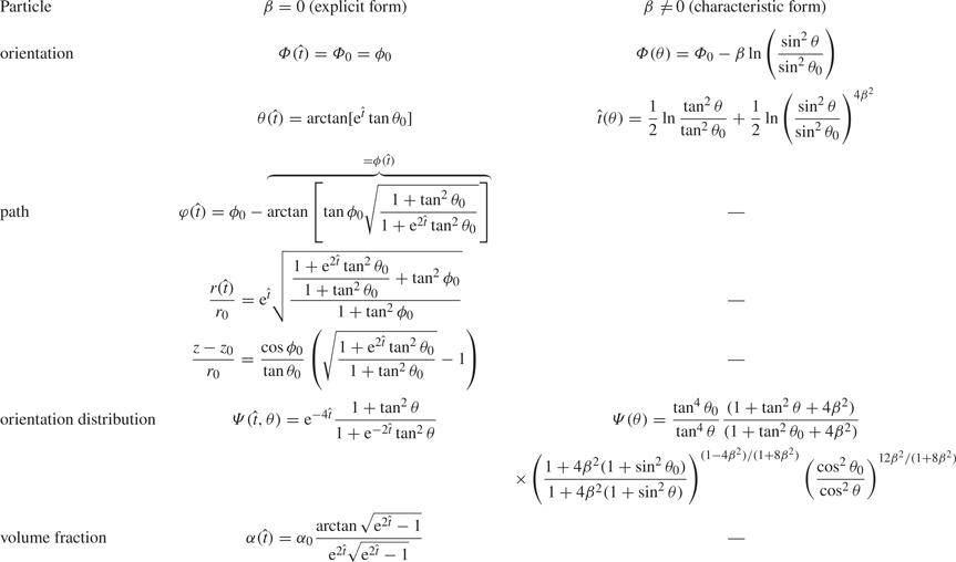
3.4. The development of  $\varPsi$

Using the analysis so far we can now be more explicit in the formulation of the Fokker–Planck equation (2.18). Since  $\boldsymbol {v}=\boldsymbol {u} + \boldsymbol {v}_R$, $\dot {\varphi } =({1}/{r})\boldsymbol {v}\boldsymbol {\cdot } \boldsymbol {\hat {e}}_\varphi = ({1}/{r})(\boldsymbol {u} + \boldsymbol {v}_R) \boldsymbol {\cdot } \boldsymbol {\hat {e}}_\varphi$ and $\boldsymbol {\dot {p}}=\boldsymbol {\dot {p}}_{fluid} + \boldsymbol {\dot {p}}_R=(\boldsymbol {\omega } + \boldsymbol {\xi }_R) \times \boldsymbol {p}$, we get
 \begin{equation} \stackrel{\circ}{\boldsymbol{p}}= \boldsymbol{\dot{p}} - \dot{\varphi} \boldsymbol{\hat{k}} \times \boldsymbol{p}= \left(\boldsymbol{\omega} - \frac{u_\varphi}{r}\boldsymbol{\hat{k}}+ \boldsymbol{\xi}_R- \frac{v_{R,\varphi}}{r} \boldsymbol{\hat{k}}\right) \times \boldsymbol{p}. \end{equation}
It turns out (see the next subsection) that the secondary fluid motion generated by a homogeneous suspension in an infinitely long circular cylindrical geometry is a weak retrograde solid body rotation relative to the rapidly rotating container with a uniform vorticity of magnitude  $\varepsilon \alpha \varOmega$. For a solid body rotation, all fluid line elements, independent of position, rotate at the same rate such that $\boldsymbol {\dot {p}}_{fluid}=\boldsymbol {\omega }\times \boldsymbol {p}= ({u_\varphi }/{r})\boldsymbol {\hat {k}}\times \boldsymbol {p}$ whereby (3.18) reduces to
 \begin{equation} \stackrel{\circ}{\boldsymbol{p}}= \left( \boldsymbol{\xi}_R- \frac{v_{R,\varphi}}{r} \boldsymbol{\hat{k}}\right) \times \boldsymbol{p}. \end{equation}
Alternatively, if the secondary motion is not a solid body rotation, such as in a non-circular geometry, (3.19) holds approximately if the relative magnitude  $\varepsilon \alpha$ is much smaller than that of the relative velocity of the particles $\varepsilon \beta$, i.e. $\alpha \ll \beta$. We then rescale (2.18) according to new variables
 \begin{equation} \hat{t}= \varepsilon \beta t, \quad \boldsymbol{\hat{u}}=\frac{\boldsymbol{u}}{\varepsilon \beta}, \quad \boldsymbol{\hat{v}}_R=\frac{\boldsymbol{v}_R}{\varepsilon \beta}, \end{equation}
to obtain
 \begin{equation} \frac{\mathrm{D} \varPsi}{\mathrm{D} \hat{t}} + \varPsi \left[ \boldsymbol{\nabla} \boldsymbol{\cdot} \boldsymbol{\hat{u}} + \boldsymbol{\nabla} \boldsymbol{\cdot} \boldsymbol{\hat{v}}_R + \boldsymbol{\nabla}_p \boldsymbol{\cdot} \hat{\stackrel{\circ}{\boldsymbol{p}}} \right]=0, \end{equation}
where the total time derivative in physical and orientation space is
 \begin{equation} \frac{\mathrm{D} \varPsi}{\mathrm{D} \hat{t}}=\frac{\partial \varPsi}{\partial \hat{t}} + (\boldsymbol{\hat{u}} + \boldsymbol{\hat{v}}_R) \boldsymbol{\cdot} \boldsymbol{\nabla} \varPsi + \hat{\stackrel{\circ}{\boldsymbol{p}}} \boldsymbol{\cdot} \boldsymbol{\nabla}_p \varPsi. \end{equation}
One may note here that, from the definition of  $\boldsymbol {v}_R=\boldsymbol {v}-\boldsymbol {u}$ and conservation of volume, it follows that $\boldsymbol {\nabla } \boldsymbol {\cdot } (\boldsymbol {u} - \varepsilon \alpha \boldsymbol {v}_R)=0$. The first term in the bracket of (3.21) is therefore neglected to lowest order in $\varepsilon$. Then it is shown (see Appendix B) that the remaining parts of the bracket in (3.21) can be written
 \begin{equation} [\boldsymbol{\nabla} \boldsymbol{\cdot} \boldsymbol{\hat{v}}_R + \boldsymbol{\nabla}_p \boldsymbol{\cdot} \hat{\stackrel{\circ}{\boldsymbol{p}}}]=\frac{2 + \sin^2 \theta}{1+4\beta^2 (1+\sin^2 \theta)} +\frac{1}{\sin \theta}\frac{\mathrm{d}}{\mathrm{d}\theta}(\sin \theta\, \hat{\dot{\theta}}), \end{equation}
where  $\hat {\dot {\theta }}$ is a function of $\theta$ given by (3.10). Thus, the sum of the divergences is independent of the spatial position $\boldsymbol {r}$ as well as of the azimuthal orientation angle $\phi$. Therefore, for an initially uniform distribution, i.e. $\varPsi (\hat {t}=0, r, \varphi, \theta, \phi )=1$, there is no source in (3.21) to render $\varPsi$ dependent on $\boldsymbol {r}$ and $\phi$. The time dependent solution then depends only on $\hat {t}$ and $\theta$, with $\boldsymbol {\nabla } \varPsi = 0$ and $\partial \varPsi / \partial \phi =0$. From (3.21), (3.22), (3.23) and (3.10) we get
 \begin{align} \frac{\mathrm{d} \varPsi(\hat{t}, \theta(\hat{t}))}{\mathrm{d} \hat{t}} & = \frac{\partial \varPsi}{\partial \hat{t}} +\frac{\mathrm{d}\theta}{\mathrm{d}\hat{t}}\frac{\partial \varPsi}{\partial \theta}\nonumber\\ & ={-}\varPsi \left[ \frac{2 + \sin^2 \theta}{1+4\beta^2 (1+\sin^2 \theta)}+\frac{1}{\sin \theta}\frac{\mathrm{d}}{\mathrm{d}\theta}(\sin \theta\, \hat{\dot{\theta}}) \right], \end{align}
 \begin{align} \hat{\dot{\theta}} & = \frac{\mathrm{d}\theta}{\mathrm{d}\hat{t}} = \frac{\sin \theta \cos \theta}{1+4 \beta^2 \cos^2 \theta} . \end{align}
Equations (3.24) and (3.25) are now in characteristic form where the path,  $\theta (\hat {t})$, is given by the inverse of (3.13). The solution for $\varPsi$ can then be obtained from an ordinary differential equation along this path. The analysis is given in detail in Appendix C and the analytical expression in characteristic form found is given in table 2. From these expressions it is a straightforward procedure to obtain $\varPsi (\hat {t}, \theta )$ for any given pair of $\hat {t}, \theta$ by first finding the corresponding value of $\theta _0$ from (3.13) by numerical iteration, and using this result in (C5) with $\varPsi _0=1$.
For  $\beta \rightarrow 0$ the solution can be reduced to an explicit expression for $\varPsi (\hat {t}, \theta )$ by direct elimination of the initial angle, $\theta _0$, from the characteristic solution (C5)
 \begin{equation} \varPsi (\hat{t}, \theta)= {\rm e}^{{-}4\hat{t}}\frac{1+ \tan ^2 \theta}{1+{\rm e}^{{-}2\hat{t}}\tan ^2 \theta } . \end{equation}
This represents the basic solution for the orientation distribution as  $\beta \rightarrow 0$, i.e. when the centrifugal acceleration is the only inertial force accounted for. The total volume fraction of rod particles, independent of orientation direction, is obtained by integration of (2.15) over the unit sphere using (3.26). For the normalised volume fraction we obtain in the case $\beta =0$ the explicit expression
 \begin{align} \frac{\alpha(\hat{t})}{\alpha_0}=\frac{1}{4 {\rm \pi}} \int_0^{2{\rm \pi}} \int_0^{\rm \pi} \varPsi (\hat{t}, \theta) \sin \theta \,\mathrm{d} \theta \,\mathrm{d} \phi= \frac{{\rm e}^{{-}2\hat{t}}}{2} \int_0^{\rm \pi} \frac{1+ \tan ^2 \theta}{{\rm e}^{2\hat{t}}+\tan ^2 \theta }\sin \theta \,\mathrm{d} \theta = \frac{\arctan{\sqrt{{\rm e}^{2\hat{t}}-1}}}{{\rm e}^{2\hat{t}} \sqrt{{\rm e}^{2\hat{t}}-1}}. \end{align}
For large times,  $\hat {t} \gg 1$, (3.27) approaches $\alpha (\hat {t})/\alpha _0=({{\rm \pi} }/{2}) {\rm e}^{-3\hat {t}}$, whereas the maximum of (3.26), at $\theta ={\rm \pi} /2$, approaches ${\rm e}^{-2\hat {t}}$.
3.5. The secondary motion of the mixture
Following Greenspanh (Reference Greenspanh1988) for the generation of vorticity in a uniform suspension of particles, initially at rest relative to a rapidly rotating cylindrical container, one finds that the potential vorticity of the mixture remains constant in time and space, i.e.
 \begin{equation} \frac{\mathrm{d}}{\mathrm{d}t}\left(\frac{\zeta_z(t) + 2\varOmega}{\rho_f(1+\epsilon \alpha(t))}\right)=0, \end{equation}
where  $\zeta _z=(\boldsymbol {\nabla } \times \boldsymbol {u}) \boldsymbol {\cdot } \hat {\boldsymbol {k}}$ is the vertical vorticity component of the fluid particle mixture. Thus
 \begin{equation} \frac{\zeta_z(t) + 2\varOmega}{1+\epsilon \alpha(t)}=\frac{2\varOmega}{1+\epsilon \alpha_0}, \end{equation}
whereby
 \begin{equation} \zeta_z(t)={-}2\varOmega \epsilon \frac{(\alpha_0-\alpha(t))}{1+\epsilon \alpha_0}. \end{equation}
For the uniform vorticity in a circular cylinder  $({\boldsymbol {u} \boldsymbol {\cdot } \hat {\boldsymbol {e}}_\varphi })/{r} = \dot {\varphi }_{fluid}(t)={\zeta _z(t)}/{2}$. Scaling with the separation time, $1/(\varOmega \epsilon \beta )$, and assuming $\epsilon \alpha _0 \ll 1$, (3.30) then yields
 \begin{equation} \hat{\dot{\varphi}}_{fluid}(t)=\frac{\hat{\zeta}_z(t)}{2}={-}\frac{\alpha_0}{\beta} (1-\frac{\alpha(t)}{\alpha_0}), \end{equation}
or equivalently
 \begin{equation} \hat{\dot{\boldsymbol{p}}}_{fluid}={-}\frac{\alpha_0}{\beta} \left(1-\frac{\alpha(t)}{\alpha_0}\right) \hat{\boldsymbol{k}} \times \boldsymbol{p}. \end{equation}
Apparently, this secondary motion of the fluid mixture in a circular cylinder is a time dependent, retrograde, solid body rotation. The negative angular velocity  $\hat {\dot {\varphi }}_{fluid}$ adds to the particle path's azimuthal velocity in (3.15). This effect is investigated for one of the cases of particle paths in the next section. (We may also note that the Rossby number of this secondary motion is $Ro=U/(\varOmega R)=\epsilon \alpha _0 \ll 1$.)
4. Results
We first discuss the change of orientation of single rod particles at different initial orientations and at different values of the particle Taylor number as obtained from the analytical solutions in (3.12) and (3.13). The upper parts of figure 5 and figure 6 show the development of the polar angle  $\theta$ vs non-dimensional time $\hat {t}$ for the initial polar angles ${\rm \pi} /8$ and ${\rm \pi} /4$, respectively. As expected, the apparent centrifugal force field turns the fibre towards increasing polar angles. It is noted that the rate of change of the polar angle is independent of the azimuthal angle, as is also clear from (3.10). The value of the polar angle asymptotically approaches ${\rm \pi} /2$, i.e. independent of initial orientation (except for $\theta _0=0$) the rod particle aligns with the plane perpendicular to the rotation axis. For increasing values of the particle Taylor number $\beta$ this asymptotic approach is delayed in non-dimensional time units, and particularly so for smaller initial polar angles. The relative magnitude of the gyroscopic to the viscous torques, associated with the rotation of the particle relative to the container, is measured by $\beta$, as apparent in (3.6). One can also understand this gyroscopic effect as a manifestation of the torque obtained from the apparent Coriolis force distribution on infinitesimal filaments along the rod particle associated with the change of orientation of the rod particle. Thus, the gyroscopic effects for non-zero $\beta$ (non-zero Coriolis acceleration) make the rod particle turn also in the azimuthal plane, and at the cost of slower alignment with the horizontal plane.

Figure 5. Orientation angles,  $\theta /{\rm \pi}$: —, and $(\varPhi -\varPhi _0)/|\Delta \varPhi |$: - - -, vs time for initial polar angle $\theta _0={\rm \pi} /8$ and $\beta =0, 0.4, 0.8$. Inset: corresponding paths of the orientation vector, $\boldsymbol {p}$, on the unit sphere.

Figure 6. Orientation angles,  $\theta /{\rm \pi}$: —, and $(\varPhi -\varPhi _0)/|\Delta \varPhi |$: - - -, vs time for initial polar angle $\theta _0={\rm \pi} /4$ and $\beta =0, 0.4, 0.8$. Inset: corresponding paths of the orientation vector, $\boldsymbol {p}$, on the unit sphere.
Figure 7 shows the total turning of the rod particle relative to the container in the azimuthal plane vs the initial polar angle  $\theta _0$ and for different values of the particle Taylor number. For $\beta \rightarrow 0$, i.e. as the apparent torque from the relative rotation is completely neglected, the rod particle keeps its initial orientation relative to the container as projected in the azimuthal plane. As the particle Taylor number is increased the rod particle turns relative to the container in the direction opposite to the main direction of rotation. The total turning angle $\Delta \varPhi$ is approached asymptotically as the fibre simultaneously aligns with the azimuthal plane. As can be seen in figure 7, $\Delta \varPhi$ is larger in magnitude for cases with smaller initial polar angle. This is because the time period required to align with the azimuthal plane, and thereby the associated period of turning in the azimuthal plane, is longer. This is also apparent in the insets of figure 5 and figure 6, which illustrate the paths of the orientation vector, $\boldsymbol {p}$, on the unit sphere for different values of $\beta$ at the given initial angle $\theta _0$. The lower parts of figures 5 and 6 show the change of the azimuthal angle vs the non-dimensional time $\hat {t}$ normalised with the magnitude of the total azimuthal turning angle $|\Delta \varPhi |=\beta \ln (1/\sin ^2 \theta _0)$. Note that the normalisation includes a factor $\beta$ so that the graphs indicated the relative effect on the asymptotic approach to the final azimuthal angle for any value of $\beta$. In parallel with the delayed approach of alignment with the azimuthal plane of the rod particle in non-dimensional time units, increasing values of the particle Taylor number delay also the approach to the final azimuthal angle.

Figure 7. Maximum change of orientation angle  $\Delta \varPhi = -\beta \ln (1/\sin ^2 \theta _0)$ vs $\theta _0$ for $\beta =0, 0.1, 0.2, 0.4, 0.8$.
Figure 8 shows particle paths and selected particle projections (not to scale in any of the figures) in the azimuthal plane at particle Taylor number  $\beta \rightarrow 0$ for different initial orientations. The initial orientations considered are also displayed in figure 3, from a viewpoint along the $x$-axis looking towards the origin. In figure 8 the fibre initial position appears as an asterisk when viewed from a distant position. For this case the azimuthal angle relative to the container $\varPhi$ is constant, but as the particles sediment also in the angular direction, $\varphi$, the azimuthal orientation of the particles, $\phi$, relative to the position vector $\boldsymbol {r}$ change and finally the particles end up at $\phi =0$ aligned with the path line, settling only in the radial direction. Exceptions from this behaviour can be observed for $\varPhi =\pm {\rm \pi}/2$, when the particles keep their orientations perpendicular to the altogether radial path lines. Figure 9(a) shows the corresponding vertical position vs the radial distance $r$. For orientation vectors $\boldsymbol {p}$ perpendicular to the direction of sedimentation at $\varPhi =\pm {\rm \pi}/2$ there are, as expected, no vertical deflections of the path lines for the chosen initial polar angle $\theta _0={\rm \pi} /6$. However, for all other values of $\varPhi$ the particles follow path lines with a vertical deflection nonlinearly associated with the orientation of $\boldsymbol {p}$. For a small, but non-zero particle Taylor number, as in figure 9(b), the vertical deflections of the paths at $\varPhi _0=\pm {\rm \pi}/2$ are non-zero too, since the settling velocity, as explained below, now has a component also in the negative $\varphi$-direction, tangential to the projection of $\boldsymbol {p}$ in the azimuthal plane.

Figure 8. Particle paths in the azimuthal plane for initial polar angle  $\theta _0={\rm \pi} /6$, and different azimuthal angles $\varPhi$ for $\beta =0$. Corresponding projections (not to scale in any figure) of the fibre in the horizontal plane at $\hat {t}=0, 0.8, 1.4, 2.0, 2.6, 3.3 .$ Inset: flow lines of the particle orientation velocity vector, $\stackrel {\circ }{\boldsymbol {p}}$, on the upper part of the unit sphere relative the direction of the position vector, $\boldsymbol {e_r}(\hat {t})$, of a moving particle.

Figure 9. Vertical position  $z/r_0$ of particle paths vs $r/r_0$ for initial polar angle $\theta _0={\rm \pi} /6$, and different initial azimuthal angles $\varPhi _0$, for $\beta =0$ (a), and $\beta =0.01$ (b).
In figure 10 we show the paths obtained for a small, non-zero particle Taylor number  $\beta =0.05$. The Taylor number, $\beta$, is also a measure of the apparent Coriolis force to the viscous drag associated with the centre of mass motion of the particle relative to the container, as apparent in (3.2). The symmetry of the paths with respect to the initial azimuthal angle is now broken. The purely radial paths obtained at $\beta =0$ for initial azimuthal angles $\varPhi _0=0, \pm {\rm \pi}/2$ are replaced by paths deflected towards negative $\varphi$ due to the effect of the Coriolis acceleration. Paths for other values of $\varPhi _0$ are deflected analogously in comparison with the paths in figure 8. We observe from (3.15) that the rate of change of direction of $\boldsymbol {r}$, i.e. $\hat {\dot {\varphi }}$, for a particle along its path asymptotically can approach zero when $\theta \rightarrow {\rm \pi}/2$ as long as $\beta \le 1/8=0.125$. The corresponding asymptotic value of the azimuthal orientation angle relative to $\boldsymbol {r}$ is then $\phi _\infty =\tfrac {1}{2} \arcsin 8 \beta$, or alternatively $\phi _\infty =\tfrac {1}{2} \arcsin 8 \beta + {\rm \pi}$ depending on the initial orientation $\varPhi _0$. In figure 10 only the particle with initial orientation angle $\varPhi _0={{\rm \pi} }/{2}$ approaches the latter state, which appears identical to the particle with $\varPhi _0=-({{\rm \pi} }/{2})$ in the projected plane. Thus, particles also in this case of the particle Taylor number approach radial path lines but with the orientation vector $\boldsymbol {p}$ misaligned with $\boldsymbol {r}$, which compensates the retrograde angular drift due to the Coriolis acceleration. The angular directions of these asymptotic path lines, as compared with the initial position $\boldsymbol {r}_0$, are given by $\varphi _\infty =\varPhi _0-\beta \ln ({1}/{\sin ^2 \theta _0})-\phi _\infty$. There is also the possibility that $\hat {\dot {\varphi }}$ asymptotically approaches zero as $\phi \rightarrow \phi _\infty '=\pm ({{\rm \pi} }/{2})-\tfrac {1}{2} \arcsin 8 \beta$, but there is only one flow line on the upper unit sphere leading to each of these asymptotic states. The position of the stagnation points at $\theta ={\rm \pi} /2$, $\phi =\tfrac {1}{2} \arcsin 8\beta$ and $\phi ={{\rm \pi} }/{2} - \tfrac {1}{2} \arcsin 8\beta$ are also visible from the flow lines of figures 8 and 10 (insets). Note that the flow field on the unit sphere is not solenoidal, as also concluded explicitly in Appendix B.

Figure 10. Particle paths in the azimuthal plane for initial polar angle  $\theta _0={\rm \pi} /6$, and different initial azimuthal angles $\varPhi _0$ for $\beta =0.05$. Corresponding projections of the fibre in the horizontal plane at $\hat {t}=0, 0.8, 1.4, 2.0, 2.6.$ Inset: flow lines of the particle orientation velocity vector, $\stackrel {\circ }{\boldsymbol {p}}$, on the upper part of the unit sphere relative the direction of the position vector, $\boldsymbol {e_r}(\hat {t})$, of a moving particle.
The limiting case at which radial asymptotic path lines are observed, i.e. for  $\beta =0.125$, is shown in figure 11. The azimuthal orientation angles relative to $\boldsymbol {r}$ of the asymptotic states are then $\phi _\infty ={\rm \pi} /4$ for a majority of the path lines shown. Although for initial azimuthal angles $\varPhi _0={{\rm \pi} }/{2}$ and $\varPhi _0={{\rm \pi} }/{3}$ the upper end of the rod particles are finally oriented in the opposite direction $\phi _\infty ={\rm \pi} /4+{\rm \pi}$. For all paths the approach to the final azimuthal orientation relative to the container, $\varPhi _\infty =\varPhi _0-\beta \ln ({1}/{\sin ^2 \theta _0})$, is a relatively rapid process, as also illustrated in figures 5 and 6. However, the rapidity of the approach to the final radial path lines is quite different depending on the initial azimuthal orientation. This is particularly illustrated by the path line for $\varPhi _0={{\rm \pi} }/{3}$ for which the final azimuthal direction is approximately $\varphi _\infty \approx -{\rm \pi}$. To reach this state, at $\phi _\infty ={\rm \pi} /4+{\rm \pi}$, $\theta _\infty ={\rm \pi} /2$, the rapid alignment with, and turning in the azimuthal plane at the beginning of the path, is followed by a large deflection of the path in the retrograde azimuthal direction. In this later part of the path the particle's orientation relative to the container is essentially the same, and the azimuthal drift continues until the final orientation relative to $\boldsymbol {r}$ is reached. Thus, in the figure shown, only the very first phase of this process is illustrated for the path with $\varPhi _0={{\rm \pi} }/{3}$. In the inset of figure 11 one may identify three flow lines on the unit sphere illustrating this type of approach to the final orientation state relative to $\boldsymbol {r}$. As can be seen the four stagnation points of the flow lines on the unit sphere (at $\theta ={\rm \pi} /2$) for smaller particle Taylor number have here merged into two for this particular value of $\beta$.

Figure 11. Particle paths in the azimuthal plane for initial polar angle  $\theta _0={\rm \pi} /6$, and different initial azimuthal angles $\varPhi _0$ for $\beta =0.125$. Corresponding projections of the fibre in the horizontal plane at $\hat {t}=0, 0.8, 1.4, 2.0, 2.6, 3.3.$ Inset: flow lines of the particle orientation velocity vector, $\stackrel {\circ }{\boldsymbol {p}}$, on the upper part of the unit sphere relative the direction of the position vector, $\boldsymbol {e_r}(\hat {t})$, of a moving particle.
If the particle Taylor number is larger than  $\beta =0.125$ the paths continuously deflect in the retrograde azimuthal direction in a spiralling fashion. To visualise this figure 12, at $\beta =0.25$, covers larger distances from the initial position of the fibre paths. All of the orientation flow lines of $\stackrel {\circ }{\boldsymbol {p}}$ (inset) here approach the limit of a circle in the azimuthal plane.

Figure 12. Particle paths in the azimuthal plane for initial polar angle  $\theta _0={\rm \pi} /6$, and different initial azimuthal angles $\varPhi _0$ for $\beta =0.25$. Corresponding projections of the fibre in the horizontal plane at $\hat {t}=0, 0.8, 1.5, 2.1, 2.7, 3.3, 4.0.$ Inset: flow lines of the particle orientation velocity vector, $\stackrel {\circ }{\boldsymbol {p}}$, on the upper part of the unit sphere relative the direction of the position vector, $\boldsymbol {e_r}(\hat {t})$, of a moving particle.
As can be seen in figure 13(b) for the vertical positions along the paths, at least four of the paths for  $\beta =0.25$ represent particles which turn their lower ends in the settling direction, resulting in a negative drift velocity in the vertical direction. For $\beta =0.125$ in figure 13(a) only two of the displayed paths represent similar trends. We note that the vertical drifts appear larger at smaller values of the particle Taylor number.

Figure 13. Vertical position  $z/r_0$ of particle paths vs $r/r_0$ for initial polar angle $\theta _0={\rm \pi} /6$, and different initial azimuthal angles $\varPhi _0$, for $\beta =0.125$ (a), and $\beta =0.25$ (b).
To complete the picture we also present particle paths that include the weak secondary fluid motion in a circular cylinder, the effect of which is most easily illustrated as modifications to the particle paths for the case presented in figure 8 for the limit  $\beta \rightarrow 0$. By including a secondary fluid motion of relative magnitude $\alpha _0/\beta =0.1$ in figure 14, the symmetry of the paths in figure 8 is now broken due to the superposed retrograde rotation of the paths. In particular one notes that the paths for $\varPhi _0=0$ and $\varPhi _0=\pm {\rm \pi}/2$ no longer coincide. The instantaneous azimuthal orientation angle, $\phi$, relative to the position vector of the particle is not changed as the secondary motion is accounted for.

Figure 14. Particle paths including the time dependent, secondary motion of the suspension at relative magnitude  $\alpha _0/\beta =0.1$ for the case in figure 8.
From here on we turn the discussion to the results for the development of the orientation distribution function, for which an analytical solution is available for any value of the particle Taylor number  $\beta$. The orientation distribution function obtained reflects the statistical appearance of particle positions and orientations that develop for an initially uniform suspension in physical and orientation space. The position of the particles continues to be uniformly distributed (away from the thickening region close to the boundary of the cylinder) for all times, whereas their orientation, as we have seen, aligns with the horizontal plane at polar angle $\theta ={\rm \pi} /2$. Figure 15 displays the limit $\beta \rightarrow 0$ at different non-dimensional times. It illustrates the alignment of the rod particles with the horizontal plane, i.e. towards $\theta ={\rm \pi} /2$, due to the non-balanced rate of change of angular momentum of the rod particles in the non-rotating frame of reference. The overall level of $\varPsi$ also decreases due to the divergent nature of the particle velocity relative to the container. It might be surprising that the orientation distribution function is independent of $\phi$ despite the fact that we already concluded that particles asymptotically end up aligned with radial path lines, at $\phi =0$, for this limit of the particle Taylor number. However, particles aligned with the path lines settle faster in the divergent velocity field than particles in other classes, which apparently compensates for the accumulation of particles in this class due to alignment. The case of a finite particle Taylor number, $\beta =0.25$, is shown in figure 16. The decay rate of $\varPsi$ in the non-dimensional time unit here appears lower, and the peak more narrow, as compared with the case of lower particle Taylor number.

Figure 15. Orientation distribution,  $\varPsi (\hat {t}, \theta )$, vs $\theta$ for $\beta =0$ at different non-dimensional times $\hat {t}$.

Figure 16. Orientation distribution,  $\varPsi (\hat {t}, \theta )$, vs $\theta$ for $\beta =0.25$ at different non-dimensional times $\hat {t}$.
The development of the normalised volume fraction of particles, as integrated from all possible orientation angles, is shown in figure 17 for different values of the particle Taylor number. Similar to reported results for spherical particles, see e.g. Dahlkild & Greenspan (Reference Dahlkild and Greenspan1989), there is an exponential decay due to the divergent relative velocity field of the particles. For increasing particle Taylor number the decay rates are smaller as measured in non-dimensional time units characteristic to the overall separation process. Note, however, that measured on the physical time scale,  $t'$, the results might be different since the characteristic non-dimensional time unit, $\hat {t}=\varepsilon \beta \varOmega t'$, is compressed by scaling with the particle Taylor number. In figure 18 we display the development of the volume fraction vs, $({\varOmega t'}/{2{\rm \pi} })\varepsilon =\hat {t}/(2{\rm \pi} \beta )$, i.e. vs the number of revolutions of the container times the small relative density difference. What is clear then from this graph is that, for small $\beta$, the rate of separation is indeed quite slow compared with larger values of $\beta$. In addition, it also becomes clear that there exists an optimal value of the particle Taylor number, $\beta \approx 0.4$, for which separation to a certain level requires the smallest number of revolutions. From a physical point of view, the explanation is that the effect of the apparent Coriolis force due to the relative motion (and rotation), which relative magnitude compared with the viscous force is measured by $\beta$, makes the particles go partly perpendicular rather than parallel to the centrifugal force. Thus, a small value of $\beta$ diminishes this effect. However, a smaller value of $\beta$, representing dominating viscous forces, also gives a longer separation time $\sim 1/(\varOmega \epsilon \beta )$. Thus, an intermediate value of $\beta$ for optimal efficiency is expected. In fact, from (3.3) we can make a more precise estimate of the relative radial settling speed. For a fibre oriented along $\boldsymbol {r}$, e.g., we have $\phi =0$, $\theta ={\rm \pi} /2$, which with (3.4a,b) gives a dimensional relative radial velocity $\sim 2 \varOmega R \epsilon \beta /(1+8 \beta ^2)$. The corresponding estimate of the separation time is then proportional to $(1+8 \beta ^2)/\beta$, which has a minimum at $\beta _{opt}={1}/{2 \sqrt {2}}\approx 0.35$, quite close to the estimate given above.

Figure 17. Normalised volume fraction: —, and  $({{\rm \pi} }/{2}){\rm e}^{-3\hat {t}}$: - - -, vs non-dimensional time $\hat {t}$.

Figure 18. Normalised volume fraction vs scaled number of container revolutions  $\varepsilon {\varOmega t'}/{2{\rm \pi} }=\hat {t}/(2{\rm \pi} \beta )$; $\beta =0{,}01, 0{.}1, 0{,}2, 0{,}3$: - - -, $\beta =0{,}4$: —, $\beta =0{,}5$: $\cdots$, $\beta =0{,}6$: – - –.
Finally, we investigate the normalised probability density of finding particles at a certain polar angle  $\theta$. Thus, at $\hat {t}=0$, as $\varPsi =1$, in figure 19, the probability density is just $\sin \theta$, reflecting the circumferential length of an infinitesimal area $2{\rm \pi} \sin \theta \, \mathrm {d} \theta$ on the unit sphere in orientation space enclosing the polar axis. As time proceeds the area under all graphs of figure 19 is the same, showing the accumulation of particles with orientation close to $\theta ={\rm \pi} /2$. At the same non-dimensional times $\hat {t}$ the height and narrowness of the peaks are accentuated for increasing particle Taylor number.

Figure 19. Normalised global orientation distribution vs  $\theta$ at different non-dimensional times $\hat {t}$; $\beta =0$: —, and $\beta =0{,}25$: - - -.
5. Conclusion
We considered the centrifugal separation of rod particles in the Stokes flow regime. In addition to the centrifugal acceleration, first-order effects of the Coriolis acceleration on the relative translation and gyroscopic effects on the relative rotation of the rod particles were accounted for and measured in terms of a non-zero modified particle Taylor number. In the limit of small (zero) particle Taylor number, the particles aligned with the plane perpendicular to the axis of rotation without changing their azimuthal orientation relative to the container. For non-zero particle Taylor number, the particles also turned in the azimuthal plane to a degree independent of the initial azimuthal orientation. We also found that, if the particle Taylor number was less or equal to  $1/8$, the resulting path lines of settling fibres in the plane perpendicular to the rotation axis asymptotically approached radial lines, whereas, for larger values of the particle Taylor number, particles continued to drift in the retrograde angular direction relative to the rotating container while still approaching a fixed asymptotic azimuthal orientation.
Regarding the development of the orientation distribution function, we presented an analytical solution in the case of an initially homogeneous, well-mixed suspension of particles in physical and orientation space, which showed that the distribution of the particles orientation remained independent of the azimuthal orientation angle. However, there was an accumulation of particles oriented parallel to the horizontal plane which was emphasised as the particle Taylor number increased.
The result for the orientation distribution function is far from intuitively trivial if we, e.g. address the behaviour of the asymptotic path lines of the fibres for large times. For the smaller values of the particle Taylor number studied, the particles approached radial path lines with orientation almost aligned with  $\boldsymbol {r}$. Thus, for large times one might expect a peak in the orientation distribution function for a small azimuthal angle relative to $\boldsymbol {r}$. As our results show, this is not the case. Apparently fibres with initial orientations that are first to reach alignment with $\boldsymbol {r}$ can settle more rapidly than fibres with other initial orientations which have not reached alignment with $\boldsymbol {r}$. This compensates for the apparent cumulative addition to the fraction of fibres aligned with $\boldsymbol {r}$, as the fractions of already aligned fibres decrease more rapidly in the centrifugal field than those not aligned.
The volume fraction of particles, disregarding their orientation, decreased exponentially with time due to the divergent velocity field relative to the rotating fluid. We also found an optimal value of the particle Taylor number,  $\beta _{opt}=0.4$, with respect to the number of revolutions of the container required to reach a certain degree of separation. Note, however, that effects of the Coriolis acceleration were not accounted for in the detailed flow around the particle related to the local frictional force and torque acting on the particle. Therefore, for larger values of the particle Taylor number, the calculation of these forces and torques would need to be reconsidered. This is probably the most important inertial effect that is not covered by the Stokes limit considered here, meaning that the extended models including inertial forces of the detailed flow around the rod particle developed for the case of gravitational settling are not sufficient for centrifugal settling.
Another critical aspect is the stability of the present solution with respect to density perturbations, as already considered in the literature for the case of gravitational settling of an initially uniform suspension of rod-like particles, both experimentally and theoretically. The effect of the retrograde secondary motion of the particle liquid mixture as a whole, as addressed here for the case of a circular cylinder, will require an extended analysis for a non-circular container, since then the additional rotation rate of the fibres in the azimuthal plane from the bulk motion is not uniform, neither in physical nor in orientation space. The analysis of the present paper could probably be extended also to more general, less slender particle shapes, e.g. spheroids, although with increased algebraic complexity. Alternatively, future numerical approaches to particles in rotating flows could possibly benefit from our results, as providing a basis for benchmark tests.
Declaration of interests
The author reports no conflict of interest.
Appendix A. Particle paths for $\beta =0$

Here, we present the analysis for the particle path in the limit  $\beta \rightarrow 0$ for which an analytical solution is available. In this limit (3.12) gives that $\varPhi =\varPhi _0$, i.e. the rod does not rotate projected in the plane perpendicular to the rotation axis. Without loss of generality we suppose $\varphi (\hat {t}=0)=0$, and therefore $\phi _0=\phi (\hat {t}=0)=\varPhi _0$, whereby $\varphi =\phi _0-\phi$.
Elimination of  $\hat {t}$ between (3.10) and (3.15) for $\beta =0$ then yields
 \begin{equation} \frac{\mathrm{d} \phi}{\mathrm{d} \theta}={-} \tan \theta \sin \phi \cos \phi. \end{equation}
Applying the fact that (A1) is a separable equation we get
 \begin{equation} \frac{\tan^2 \phi}{\tan^2 \phi_0}=\frac{\cos^2 \theta}{\cos^2 \theta_0}, \end{equation}
which relates  $\phi$ to the polar angle $\theta$, given by (3.13), along the path. Now from (3.14), and using (3.10) and (3.15), respectively, to eliminate $\mathrm {d}\hat {t}$ in the two terms below, we write
 \begin{equation} \mathrm{d} \ln r=\mathrm{d}\hat{t}+\sin^2 \theta \cos^2 \phi \, \mathrm{d}\hat{t}=\frac{\mathrm{d} \theta}{\sin \theta \cos \theta} -\frac{\mathrm{d} \phi}{\tan \phi}. \end{equation}
Integration and then making use of (A2) yields
 \begin{equation} \frac{r}{r_0}=\left(\frac{\tan^2 \theta}{\tan^2 \theta_0} \frac{\sin^2 \phi_0}{\sin^2 \phi} \right)^{1/2} =\frac{\left(\dfrac{\tan^2 \phi_0}{\tan^2 \phi}-\cos^2 \theta_0\right)^{1/2}}{\sin \theta_0} \frac{\sin \phi_0}{\sin \phi}. \end{equation}
Thus, since  $\varphi =\phi _0-\phi$ (A4) is an explicit relation between $r$ and $\varphi$ along the path starting at $r=r_0, \varphi _0=0$ with given initial orientation $\theta _0, \varPhi _0=\phi _0$.
For the axial position along the path at  $\beta =0$ (3.15) and (3.16) give us with (A4)
 \begin{equation} \frac{\mathrm{d} z}{\mathrm{d} \phi}=\frac{- r}{\tan \theta \sin \phi}={-}\frac{r_0 \sin \phi_0}{\tan \theta_0}\frac{1}{\sin^2 \phi}. \end{equation}
Then
 \begin{equation} \frac{z-z_0}{r_0}=\frac{\cos \phi_0}{\tan \theta_0}\left(\frac{\tan \phi_0}{\tan \phi}-1\right). \end{equation}
By applying (3.13) at  $\beta =0$ the particle path, represented by (A2), (A4) and (A6), can also be expressed explicitly as function of time, $\hat {t}$, as summarised in table 2.
Appendix B. Derivation of (3.23)
In this appendix we shall detail how the bracket in (3.21) is simplified into (3.23). The terms of the bracket in (3.21) can be made explicit by direct calculation of the two last terms. The first term we simply neglect since  $\boldsymbol {\nabla } \boldsymbol {\cdot } \boldsymbol {\hat {u}}=\boldsymbol {\nabla } \boldsymbol {\cdot } (\varepsilon \alpha \boldsymbol {\hat {v}}_R) \ll 1$, as $\varepsilon \alpha \ll 1$. For the divergence of the relative velocity we have
 \begin{equation} \boldsymbol{\nabla} \boldsymbol{\cdot} \boldsymbol{\hat{v}}_R=\frac{1}{r} \frac{\partial}{\partial r} (\boldsymbol{\hat{v}}_R \boldsymbol{\cdot} \boldsymbol{r}) + \frac{1}{r}\frac{\partial}{\partial \varphi} (\boldsymbol{\hat{v}}_R \boldsymbol{\cdot} \boldsymbol{\hat{e}}_\varphi), \end{equation}
where the last term is zero because of symmetry. From (3.3) we get
 \begin{equation} \boldsymbol{\hat{v}}_R \boldsymbol{\cdot} \boldsymbol{r}=A r^2 (1+p_r^2) + Br^2 p_r p_\varphi, \end{equation}
and then
 \begin{equation} \frac{1}{r} \frac{\partial}{\partial r} (\boldsymbol{\hat{v}}_R \boldsymbol{\cdot} \boldsymbol{r})=2A (1+p_r^2) + 2 B p_r p_\varphi. \end{equation}
Using (3.4a,b) and (3.5a,b), (B3) can be reduced to
 \begin{equation} \frac{1}{r} \frac{\partial}{\partial r} (\boldsymbol{\hat{v}}_R \boldsymbol{\cdot} \boldsymbol{r})=2 \frac{1 + \sin^2 \theta \cos^2 \phi}{1 + 4 \beta^2 (1 + \sin^2 \theta)}. \end{equation}
For the divergence in orientation space we have
 \begin{equation} \boldsymbol{\nabla}_p \boldsymbol{\cdot} \hat{\stackrel{\circ}{\boldsymbol{p}}}= \frac{1}{\sin \theta} \frac{\partial}{\partial \theta}\left[\sin \theta \, \hat{\stackrel{\circ}{\boldsymbol{p}}} \boldsymbol{\cdot} \boldsymbol{\hat{e}_\theta} \right] + \frac{1}{\sin \theta}\frac{\partial}{\partial \phi}\left[\hat{\stackrel{\circ}{\boldsymbol{p}}} \boldsymbol{\cdot} \boldsymbol{\hat{e}_\phi}\, \right]. \end{equation}
We obtain an explicit expression of  $\hat {\stackrel {\circ }{\boldsymbol {p}}}$ via (3.19) in scaled form
 \begin{equation} \hat{\stackrel{\circ}{\boldsymbol{p}}}= ( \hat{\boldsymbol{\xi}}_R- \frac{\hat{v}_{R,\varphi}}{r} \boldsymbol{\hat{k}}) \times \boldsymbol{p}. \end{equation}
The first term of (B6) is just (3.9). The second term after simplification gives us
 \begin{align} &-\frac{1}{r}(\boldsymbol{\hat{v}}_R \boldsymbol{\cdot} \boldsymbol{\hat{e}}_\varphi) \boldsymbol{\hat{k}} \times \boldsymbol{p}={-}\left(A p_\varphi p_r + B(1 + p_\varphi^2)\right) \boldsymbol{\hat{k}} \times \boldsymbol{p}\nonumber\\ &\qquad = \frac{[-\sin^2 \theta \sin \phi \cos \phi +2 \beta (1+\sin^2 \theta)]}{1 + 4 \beta^2 (1+\sin^2 \theta)} \left( \begin{array}{@{}c@{}} 0 \\ \sin \theta \\ 0 \end{array} \right). \end{align}
We can then conclude that
 \begin{equation} \hat{\stackrel{\circ}{\boldsymbol{p}}} \boldsymbol{\cdot} \boldsymbol{\hat{e}}_\phi =\hat{\stackrel{\circ}{\boldsymbol{p}}} \boldsymbol{\cdot} \boldsymbol{\hat{e}}_y= \frac{-2 \beta \sin \theta \cos^2 \theta}{1+4 \beta^2 \cos^2 \theta} +\frac{[-\sin^2 \theta \sin \phi \cos \phi +2 \beta (1+\sin^2 \theta)]}{1 + 4 \beta^2 (1+\sin^2 \theta)}\sin \theta. \end{equation}
After differentiation and rearranging, the two terms of the divergence in orientation space are then
 \begin{gather} \frac{1}{\sin \theta}\frac{\partial}{\partial \theta}\left(\sin \theta \, \hat{\stackrel{\circ}{\boldsymbol{p}}} \boldsymbol{\cdot} \boldsymbol{\hat{e}}_\theta \right)= \frac{1}{\sin \theta}\frac{\mathrm{d}}{\mathrm{d} \theta}\left(\sin \theta \, \frac{\mathrm{d}\theta}{\mathrm{d}\hat{t}} \right), \end{gather}
 \begin{gather} \frac{1}{\sin \theta}\frac{\partial}{\partial \phi}\left(\hat{\stackrel{\circ}{\boldsymbol{p}}} \boldsymbol{\cdot} \boldsymbol{\hat{e}}_\phi \right)= \frac{- \sin^2 \theta \cos 2\phi}{1+4\beta^2 (1+\sin^2 \theta)}, \end{gather}
where in (B9) the time derivative of the polar angle is a function of  $\theta$ given by (3.10).
Summing (B4), (B9) and (B10) we can conclude after algebraic simplification
 \begin{equation} \left[ \boldsymbol{\nabla} \boldsymbol{\cdot} \boldsymbol{\hat{v}}_R + \boldsymbol{\nabla}_p \boldsymbol{\cdot} \hat{\stackrel{\circ}{\boldsymbol{p}}} \right]= \frac{2 + \sin^2 \theta}{1+4\beta^2 (1+\sin^2 \theta)}+\frac{1}{\sin \theta}\frac{\mathrm{d}}{\mathrm{d} \theta}\left(\sin \theta \, \frac{\mathrm{d}\theta}{\mathrm{d}\hat{t}} \right), \end{equation}
which is in fact independent of  $\phi$.
Appendix C. Analysis of characteristic form for orientation distribution $\varPsi$

A quadrature form of the solution could be obtained by using an alternative way of expressing (3.24). By dividing with  $\varPsi$ and rearranging we get
 \begin{equation} \frac{\mathrm{d}}{\mathrm{d} \hat{t}} \ln (\varPsi \sin \theta\, \hat{\dot{\theta}})={-}\frac{(2+ \sin^2 \theta)}{1 + 4 \beta^2 (1+\sin^2 \theta)}. \end{equation}
In this form of the conservation equation for the orientation distribution function,  $\varPsi$, the right-hand side is associated with the divergence of the velocity in physical space and the azimuthal velocity component in orientation space. This divergence acts as a sink for the relative rate of change of the flux density, $\varPsi \sin \theta \hat {\dot {\theta }}$, in the polar direction of orientation space as one follows any rod particle in its motion and change of orientation. We then eliminate $\hat {t}$ in (C1) by division with (3.25) to get
 \begin{equation} \frac{\mathrm{d}}{\mathrm{d} \theta} \ln \left(\varPsi \sin \theta \hat{\dot{\theta}}\right)=\frac{\mathrm{d}}{\mathrm{d} \theta}(\cos \theta) \left(\frac{1+ 4 \beta^2 \cos^2 \theta}{\sin^2 \theta \cos \theta}\right) \frac{(2+ \sin^2 \theta)}{1 + 4 \beta^2 (1+\sin^2 \theta)}. \end{equation}
The right-hand side can be further simplified by partial decomposition which gives
 $$\begin{gather} \displaystyle \frac{\mathrm{d}}{\mathrm{d} \theta} \ln \left(\varPsi \sin \theta\, \hat{\dot{\theta}}\right)=\frac{\mathrm{d}}{\mathrm{d} \theta}(\cos \theta) \left[ \frac{3}{(1+8\beta^2) \cos \theta}+\frac{2 \cos \theta}{1-\cos^2 \theta}\right.\nonumber\\ \left. +\left(\frac{1-4 \beta^2}{1+8\beta^2}\right)\frac{4\beta^2 \, 2 \cos \theta}{1+8\beta^2-4\beta^2 \cos^2 \theta} \right]. \end{gather}$$
Integrating (C3) along the path from an initial angle  $\theta _0$ to the current angle $\theta (\hat {t})$ we obtain, after rearranging,
 $$\begin{gather} \ln \left(\frac{\varPsi}{\varPsi_0} \frac{\sin \theta(\hat{t})}{\sin \theta_0} \frac{\hat{\dot{\theta}}(\hat{t})}{\hat{\dot{\theta}}(\hat{t}=0)}\right)= \frac{\dfrac{3}{2}}{1+8\beta^2} \ln \left(\frac{\cos^2 \theta}{\cos^2 \theta_0}\right)-\ln \left(\frac{\sin^2 \theta}{\sin^2 \theta_0}\right) \nonumber\\ - \ln \left(\frac{1+4\beta^2 (1+\sin^2 \theta(\hat{t}))}{1+4\beta^2(1+\sin^2 \theta_0)}\right)^{({1-4 \beta^2})/({1+8\beta^2})}. \end{gather}$$
From (C4) and (3.25) and using the identity  $(\cos \theta )^{-2}=1+ \tan ^2 \theta$ we finally get
 $$\begin{gather} \frac{\varPsi (\hat{t})}{\varPsi_0} = \frac{\tan^4 \theta_0}{\tan^4 \theta(\hat{t})} \frac{(1+ \tan^2 \theta(\hat{t}) + 4 \beta^2)}{(1+\tan^2 \theta_0 + 4 \beta^2)} \left(\frac{1+4\beta^2 (1+\sin^2 \theta_0)}{1+4\beta^2(1+\sin^2 \theta(\hat{t}))}\right)^{({1-4 \beta^2})/({1+8\beta^2})}\nonumber\\ \times\left(\frac{\cos^2 \theta_0}{\cos^2\theta(\hat{t})}\right)^{{12\beta^2}/({1+8\beta^2})}, \end{gather}$$
where  $\theta (\hat {t})$ is given by (3.13). It is then a straightforward procedure to obtain $\varPsi (\hat {t}, \theta )$ for any given pair of $\hat {t}, \theta$ by first finding the corresponding value of $\theta _0$ from (3.13) by numerical iteration, and using this result in (C5) with $\varPsi _0=1$.


 Open access