


Introduction
Differential high-frequency device and circuit characterization is a heavily discussed topic [Reference Veit, Gadringer and Leitgeb1]. In the literature, a number of different designs for differential load-pull systems are discussed. Some use tuners directly at the output of the device under test (DUT) and a 180° hybrid only to create the differential input signal [Reference Köther and Berben2,Reference Liu and Tsironis3]. Other approaches (compare [Reference Mahmoudi, Spirito, Valk and Tauritz4,Reference Spirito, Van der Heijden, De Kok and De Vreede5]) use 180° hybrids also at the output of the device, but only to tune the differential mode load. Mixed-mode load-pull measurement setups able to independently tune the loads of both, the common mode and the differential mode component of the output signal, were proposed in [Reference Teppati, Ferrero, Garelli and Bonino6] and [Reference Ferrero and Teppati7].
The main limitation for passive load-pull systems applying 180° hybrids at the output of the DUT is an additional insertion loss which reduces the available load tuning range. Therefore, mostly active mixed-mode load-pull systems were proposed showing all the benefits and disadvantages of such active load-pull system [Reference Mathias8]. A passive mixed-mode load-pull measurement system for an ultra-wideband ranging chip was discussed in [Reference Veit, Gadringer and Leitgeb9].
In this paper, we are extending our previous findings which were presented at the 2019 European Microwave Conference for Central Europe (EuMCE) [Reference Veit, Gadringer and Leitgeb1]. There we clarify the pros and cons of different setups using analytical derivations and load-pull measurements of a real DUT. Furthermore, we showed the theory of a new passive load-pull system with enhanced tuning capabilities. In this contribution, we shortly summarize the analytical findings from [Reference Veit, Gadringer and Leitgeb1] in section “Analytical analysis of different load-pull configurations”. Thereafter, we discuss the impact of a 180° hybrid's non-idealities on the tuning capabilities of a load-pull system in section “Impact of non-ideal 180° hybrids”. Measurement setups and results for the discussed load-configurations are presented in the sections “Measurement setups” and “Measurement results”. The conclusion in section “Conclusion” summarizes the advantages and disadvantages of each setup and provides an overview of their capabilities.
Analytical analysis of different load-pull configurations
To enable the reader to understand the presented measurement results, we shortly summarize the analytical derivations discussed in [Reference Veit, Gadringer and Leitgeb1]. We apply the generalized mixed-mode pseudo scattering parameters as described in [Reference Frei, Cai and Muller10] for these derivations. Let us consider a setup that consists of a DUT, some connection network Sc, and a load network SL as depicted in Fig. 1. The two lines coming from the differential output of the device form two ports. They can be represented by a differential mode port seeing a differential mode reflection coefficient Γdiff and a common mode port seeing a common mode reflection coefficient Γcom, or as two single-ended ports seeing reflection coefficients Γ1 and Γ2.

Fig. 1. Block diagram of a load network for a differential device.
The load network SL has only two single-ended ports named port Δ and port Σ as they will represent the impedance tuners connected to the Δ and Σ output ports of the 180° hybrid. For the observations in the sections “Direct connection to separated tuners” and “Connection via a 180° hybrid”, the tuners are terminated with a match and not connected to each other, resulting in zero transmission coefficients in the load.

To concatenate the two S-parameter blocks, the multiport T-parameter transformation from [Reference Frei, Cai and Muller10] was used to obtain Sc, SL → Tc, TL. The concatenated S-parameter block was then calculated by T = Tc ⋅ TL → S. To circumvent a division by zero, we used a generalized SL without zero transmission coefficients and perform a substitution after the inverse transformation. In the following, we investigate three different load-pull setups using the outlined framework.
Direct connection to separated tuners
Here we analyze the approach used in [Reference Köther and Berben2] and [Reference Liu and Tsironis3], where tuners are connected directly to the DUT. For this, we assume that the connection network ${\bi {S}^{\prime}}_c$ is a direct connection from port 1 to port 3 and port 2 to port 4. The connection network is perfectly matched, reciprocal, lossless, and has zero length. The results of these simplifications are shown in (2).

Using S of the concatenated network and generalized mixed-mode pseudo scattering S-parameters, we get the structure depicted in Fig. 2. Applying (2) we arrive at the result for ${\bi {S}^{\prime}}_{mix}$ shown in (3) and (4) [Reference Dobrowolski11].


Fig. 2. Block diagram of a simplified load network for a differential device using mixed-mode port representation.
The matrix entries ${S}^{\prime}_{dd}$ and ${S}^{\prime}_{cc}$
 of ${\bi {S}^{\prime}}_{mix}$
 correspond to the differential and common mode reflection coefficients the device sees. ${S}^{\prime}_{dc}$
 and ${S}^{\prime}_{cd}$
 show the mode conversion that is introduced by the load. Because ${S}^{\prime}_{dd}$
 and ${S}^{\prime}_{cc}$
 are equal, the common and differential mode loads are always the same. Additionally, mode conversion is introduced by the load if S Δ and S Σ are not equal.
Connection via a 180° hybrid
In this sub-section, we assumed that the connection network ${\bi {S}^{\prime \prime \prime}}_c$ is an ideal 180° hybrid as defined in (5). The results from (6) to (8) show that differential and common mode reflection coefficients are independent of each other, and reduce to the reflection coefficients of the tuners. Mode conversion is zero for an ideal 180° hybrid.


Direct connection to connected tuners
A third approach of mixed-mode load-pull is to connect the outputs of the tuners to each other while the inputs are connected directly to the differential output of the DUT. This approach was presented for the first time in [Reference Veit, Gadringer and Leitgeb1]. The resulting load matrix ${\bi {S}^{\prime}}_L$ provides non-zero transmission coefficients S T as highlighted in (9). Performing the same calculations as before using the assumptions from (2) and (9) results in the mixed-mode network ${\bi {S}^{\prime \prime \prime}}_{mix}$
 summarized in (10) to (12). Compared to the results in section “Direct connection to separated tuners”, now different differential and common mode reflection coefficients can be realized. Yet, they cannot be selected independently from each other. The degree in which they are depending on each other can be tuned by the transmission coefficient S T. Hence, achieving a specific combination of differential and common mode loads is more complicated compared to the load-pull approach as discussed in section “Connection via a 180° hybrid”, but no 180° hybrid is needed.


Impact of non-ideal 180° hybrids
A non-ideal 180° hybrid featuring return loss, insertion loss, phase imbalance, and magnitude imbalance as well as finite isolation causes a change of the tuning range and introduces a source of mode conversion for setups like the one shown in Fig. 3 and described in section “Connection via a 180° hybrid”. How each of the mentioned parameters affects the load tuning is being discussed in this section. For this purpose, calculations using the symbolic toolbox of Matlab® were performed. These calculations are slightly different from the ones presented in section “Connection via a 180° hybrid”, because the connection network ${\bi {S}^{\prime \prime}}_C$ is not an ideal 180° hybrid, but a hybrid with imperfections. The mathematical expressions derived using this approach are too complex to be readable and informative, thus we used plots to visualize their meaning. For this discussion, the differential input ports of the 180° hybrid are port 1 and port 2, the difference port is port 3, and the sum port is port 4, as it was already defined in (6). For demonstration of the impact, we chose a reflection coefficient of $S_{\rm \Sigma } = 0.6\;\angle 20^\circ$
 for the common mode tuner and a reflection coefficient of $S_{\rm \Delta } = 0.8\;\angle \varphi$
 with φ = 0…360° for the differential mode tuner. A comparison of the hybrid imperfection values used to create the figures in this section and values of real devices taken from Mini-Circuits® [12] can be found in Table 1. Please note that for the sake of demonstrating the impact of each individual parameter, not all chosen values have practical relevance, but were chosen to deliver readable plots.

Fig. 3. Impact of insertion loss and symmetric return loss on load tuning. S Δ (solid red line) and S Σ (blue circle) are the impedances set at the tuners. S dd, IL (dashed red line) and S cc, IL (blue cross) are the differential and common mode impedances seen by the DUT after the impact of insertion loss (IL). S dd,IL+RL (red dash-dotted line) and S cc,IL+RL (blue square) are the impedances seen by the DUT including the impact of insertion loss and symmetric return loss (RL). As mentioned in the first paragraph of section “Impact of non-ideal 180° hybrids”, the setting for the common mode load tuner is kept constant. Due to this, S Σ and S cc are only points in the chart.
Table 1. 180° hybrid imperfection values used for graphs compared with real values [Reference Dobrowolski11]

Table contains values for insertion loss (IL), return loss (RL), isolation (ISO), magnitude imbalance, and phase imbalance.
Impact of insertion and return loss
The first parameters we discuss are insertion loss (IL) and return loss (RL). By the magenta colored arrows in Fig. 4, the impact of insertion loss is visualized. As shown in (7), for an ideal 180° hybrid, the differential and common mode impedances seen by the DUT (S dd, S cc) are equal to the impedances set at the corresponding tuners (S Δ, S Σ). Insertion loss reduces the magnitude of the set reflection coefficients S Δ and S Σ, thereby limiting the available tuning range. The light blue colored arrows in Fig. 4 demonstrate the influence of symmetric return loss at the ports facing the DUT. In this context, symmetric means that the return losses at port 1 and port 2 have the same magnitude and phase (S 11 = S 22). These return losses introduce additional reflections, which add to the reflections produced by the tuners, causing a shift of S dd and S cc which depends on the magnitude and phase of the return losses. As long as S 11 and S 22 are equal, no mode conversion occurs, and the impedance shift can be compensated by changing the values of S Δ and S Σ accordingly. The same behavior is caused by return losses at the ports facing the tuners. This again can be compensated by changing the tuner settings of each individual tuner.

Fig. 4. Impact of non-symmetric return loss and poor isolation between the ports facing the DUT. S dd,IL and S dd,IL+RL (dashed red line) are the differential mode impedances seen by the DUT including the impact of insertion loss (IL) and non-symmetric return loss (RL), respectively. Similarly, S cc,IL and S cc,IL+RL (blue square) is the common mode impedance seen by the DUT including the impact of IL and non-symmetric RL, respectively. $S_{dd\comma IL + RL + ISO_{DUT}}$ (solid red line) and $S_{cc\comma IL + RL + ISO_{DUT}}$
 (blue circle) are the impedances seen by the DUT including the impact of IL, RL, and finite isolation between the DUT ports (ISODUT). S dc,IL (green cross) and S dc,IL+RL (green square) are the mode conversion seen by the DUT considering IL and non-symmetric RL. Note that mode conversion is plotted in the overlying polar plot as it cannot be mapped to an impedance value.
Figure 5 shows the impact of non-symmetric return loss (S 11 = −S 22), which means the return losses at port 1 and port 2 are 180° out of phase. This influence is depicted by the magenta colored arrow. A 180° phase difference of the return losses causes a differential mode signal to be reflected as a common mode signal and vice versa. This causes mode conversion but does not directly influence S dd and S cc. The general case where S 11 and S 22 have different magnitude and phase causes a mixture of mode conversion and shift of S dd and S cc. Different to the shift of S dd and S cc, this type of mode conversion cannot be influenced by the tuners. Therefore, we refer to this as load-independent mode conversion.

Fig. 5. Impact of poor isolation between the load ports 3 and 4 of the 180° hybrid. S dd,IL, S cc,IL, and S dc,IL are the impedances and mode conversion seen by the DUT including the impact of insertion loss. $S_{dd\comma IL + ISO_{Load}}$ , $S_{cc\comma IL + ISO_{Load}}$
 , and $S_{dc\comma IL + ISO_{Load}}$
 are the impedances and mode conversion seen by the DUT considering insertion loss and isolation. As mentioned in the first paragraph of section “Impact of non-ideal 180° hybrids”, the setting for the common mode load tuner is kept constant. But in this case, the introduced mode conversion causes $S_{cc\comma IL + ISO_{Load}}$
 to become a circle similar to the swept S dd.
Impact of finite isolation
This sub section deals with the impact of finite isolation between the isolated ports of a 180° hybrid. At first, the impact of poor isolation between the ports facing the DUT is marked by the green arrows in Fig. 5. For S cc, poor isolation causes the same shift as a symmetric return loss. This is because the incoming signals which make up the common mode signal are equal; therefore, a reciprocal transmission from port 1 to port 2 cannot be distinguished from a symmetric return loss with same phase and magnitude. The only parameter changing for S dd is the additional 180° phase shift introduced because the incoming signals at port 1 and port 2 are 180° out of phase. This causes the green arrows in Fig. 5 to point in opposite directions. This shift of S dd and S cc can be compensated by the tuners in the same way as symmetric return loss. Beside this, there is also the impact of finite isolation between the ports facing the tuners. The influence of this is shown in Fig. 6. Because of this imperfection, reflections of one tuner carry over to the other tuner, causing a coupling between the two tuners. On the one hand, this causes mode conversion which depends on the tuner settings, later referred to as load-dependent mode conversion. On the other hand, it leads to differential and common mode impedances (S dd, S cc) which now depend on both tuners (S Δ, S Σ). In the example shown in Fig. 6, this causes S cc to become a circle in the Smith chart if the phase of S Δ is swept from 0 to 2π. In order to compensate for this behavior, one would need to tune both tuners jointly, thereby losing one of the key benefits of using a 180° hybrid. Please note that especially in the case of isolation, we chose unrealistically poor values to produce readable plots. As shown in Table 1, isolation values are much better than most other imperfections and can often be neglected.

Fig. 6. Comparison of simulated and calculated impact of magnitude and phase imbalance. S dd and S cc show the differential and common mode impedances seen by the DUT. The appendixes “sim.” or “calc.” indicate the simulated points using Monte Carlo simulation or the calculated area using the simplified formulas (13) and (14). S dc shows the mode conversion due to magnitude and phase imbalance using Monte Carlo simulation only.
Impact of magnitude and phase imbalance
As last topic, we discuss the impact of magnitude and phase imbalance between the transmission parameters of a 180° hybrid. A hybrid has four transmission parameters and in general each of them may have a different magnitude and phase error relative to the ideal value. This makes it impossible to pick a single set of errors representative for all possible combinations and thus forcing us to rely on Monte Carlo simulations. For the simulations, we assumed that the magnitude errors and the phase errors are equally distributed between the given error-bounds mentioned in Table 1. This assumption is valid because we were only interested in finding an upper error bound and also assumed that the specifications are not exceeded. For this investigation, we chose a fixed S Δ of approximately −2 dB and swept the magnitude of S Σ from −15 to 0 dB. The results of this simulation using 5000 different combinations are presented in Fig. 7. As you can see, magnitude and phase imbalance causes mode conversion and a detuning of the set impedances. What you cannot see in this plot is that, similar to what we described in section “Impact of finite isolation” for poor isolation at the ports facing the tuners, imbalance is causing a dependency of the common and differential mode on both tuner settings as well as load-dependent mode conversion. To compensate these hybrid imperfections, again we would have to tune both tuners jointly.

Fig. 7. Analysis of the probability that the derived rule-of-thumb in (13) and (14) covers all possible combinations assuming the errors are uniformly distributed within the specified range. P(A ⊆ B|S Δ, S Σ) being the probability that the results of the Monte Carlo simulation (A) are a subset of the area specified by the formula (B) for a given pair of tuner reflection coefficients. To visualize this relationship, a larger number of 50 000 realizations of the Monte Carlo simulation were used. The x-axis indicates the difference in magnitude between the reflection coefficients set at the two tuners. To demonstrate the full shape of the curve, values down to −100 dB are plotted, although they cannot be realized in a real-world scenario.
Hybrid tuning error estimation
As already mentioned, we deliberately did not always use realistic values for the plots mentioned in the sections above. But in this section, we elaborate on which parameters you need to consider most when purchasing a real 180° hybrid for mixed-mode load-pull measurements. The first discussed parameter was the insertion loss which causes a significant decrease in tuning range. Especially for passive load-pull systems, this is a critical value if you aim to achieve high reflection coefficients. Differently, symmetric return loss does not decrease your tuning range, but shifts it depending on its phase and magnitude. Inside the available tuning range, this shift can be compensated with the corresponding tuner. Asymmetric return loss causes mode conversion, but with average return losses between 15 and 25 dB, the reduction in tuning range is not as severe as in the case of insertion loss. The next discussed parameter was the isolation which may cause impedance shifts, dependency of S dd and S cc on both tuners as well as load-dependent mode conversion. However, as average isolation values are rather high in a range from 23 to 35 dB, they can often be neglected compared to the impact of the other imperfections. Other than isolation, realistic values of magnitude and phase imbalance may have a severe impact on the performance of a 180° hybrid. Imbalance may cause a significant dependency of S dd and S cc on both tuners as well as load-dependent mode conversion. To compensate for this, a joint tuning of both tuners is needed, making the handling of the tuning setup much more complicated. If a joint tuning is not desired, one needs to analyze if the impact of a hybrids imperfections results in an acceptable tuning range. To assist the reader with this decision, we derived the simplified formulas (13) and (14), describing the impact of a 180° hybrid's imperfections on S dd and S cc, using the afore mentioned considerations. Compared to the ideal results of (6), these formulas include the impact of the most important imperfections, which are the IL, the magnitude error Δm, and the phase error Δφ, and were simplified to achieve an easily useable rule-of-thumb. A validation of these formulas is presented in Figs 7 and 8. To achieve this high degree of simplification, some assumptions were made. At first, isolation and return loss were neglected as the impact of isolation is small and impedance shifts due to return loss can be easily compensated. Also higher order terms and products were eliminated from the equation. At last, the different error terms were combined in a way to derive an upper error bound. Due to these simplifications, the formula does fail to deliver an upper error bound if the ratio between the magnitudes of the set reflection coefficients at the tuners is becoming larger than 20 dB as shown in Fig. 8. This is valid for realistic parameters as mentioned in Table 1. The reader can now utilize these formulas to calculate areas in the Smith chart by using the four combinations of positive and negative magnitude and phase errors. These areas indicate how S dd might change due to a change of S cc and vice versa. If the resulting area is small enough for the desired application, the reader may consider to use the corresponding 180° hybrid and independently tune S dd and S cc by using one tuner for each. Otherwise, a joint tuning of both tuners needs to be performed which is significantly more complicated and requires automatic tuner systems to be applicable in practical measurement campaigns.


Fig. 8. Load-pull setup with directly connected tuners.
Measurement setups
According to the derivations in section “Analytical analysis of different load-pull configurations”, the following setups were used to support the analytical findings with measurement results. Load-pull measurements of a real DUT were presented in [Reference Veit, Gadringer and Leitgeb1]; in this contribution, only the behaviors of the different measurement setups are investigated using an R&S ZVA 24 Vector Network Analyzer (VNA). The VNA was calibrated using an R&S Auto Calibration Unit. The reference planes for the measurements were at the input ports of the load network, which is either at the ports of the tuners or if used at the ports of the 180° hybrid.
Setup with direct connection
A load-pull setup using directly connected tuners is shown in Fig. 9. This setup does not use a 180° hybrid, but as derived in section “Direct connection to separated tuners”, it is also not able to provide different common mode and differential mode load impedances to the DUT. For the load-pull measurements in [Reference Veit, Gadringer and Leitgeb1], a spectrum analyzer was connected via an attenuator to increase the matching. For the measurements presented in this paper, a VNA was used to measure the load impedance a DUT would see.

Fig. 9. Load-pull setup with 180° hybrid.
Setup with 180° hybrid
The setup in this section utilizes a 180° hybrid as depicted in Fig. 3, similar to what was presented in [Reference Ferrero and Teppati7]. As derived in section “Connection via a 180° hybrid”, in this setup, common and differential mode loads can be set independently with the two tuners. For load-pull measurements, the output of the differential mode load tuner would be fed to a spectrum analyzer via an attenuator for better matching. For the measurement results in this paper, again a VNA was used to measure the load impedance a DUT would see.
Setup with connected tuners
Figures 10 and 11 show the measurement setup with connected tuners proposed by us in [Reference Veit, Gadringer and Leitgeb1]. In contrast to the setup depicted in Fig. 3, no 180° hybrid is used, but the ports of the tuners that do not face the DUT are now connected to each other. This connection can be adjusted in magnitude and phase. Ideally, one would use an adjustable reciprocal phase shifter with low insertion loss or a line stretcher in the connection path between the tuners, but such equipment was not available to us. To circumvent this, we used SMA female–female and male–male adapters to adjust the electrical length of the connection between the tuners. Because we were interested in the behavior of the linear load network, and not in the characterization of some DUT, an R&S ZVA VNA was used (see Fig. 10). To perform load-pull measurements with a DUT, directional couplers would be needed as shown in Fig. 11.

Fig. 10. Measurement setup used to measure the tuning behavior of the presented approach.

Fig. 11. Diagram of a load-pull setup utilizing the proposed load configuration to characterize a DUT.
Measurement results
In this section, we discuss the tuning range and behavior of each setup. For this, the screws used to tune the magnitude of each tuner's reflection coefficient were set to the same values, in a way to achieve the highest possible magnitude of the reflection coefficient. Then the position of each tuner's slide was swept and the changes to the differential and common mode reflection coefficients were captured. The results were then plotted to Smith charts. For every measurement presented in this section, a frequency of 4 GHz was used.
Results for traditional setups
Figure 12 demonstrates the difference in tuning range between direct connected tuners (see section “Direct connection to separated tuners”) and a setup using a 180° hybrid (see section “Connection via a 180° hybrid”). The maximum magnitude of the differential mode reflection coefficient for the setup with direct connected tuners is about 0.85. For the setup using a hybrid, it reduces to about 0.77. The common mode reflection coefficient without a 180° hybrid is always equal to the differential mode reflection coefficient. With a 180° hybrid, the common mode reflection coefficient can be tuned independently and was set to a low reflection coefficient of S cc = 0.025 + j 0.015.

Fig. 12. Comparison of possible differential and common mode reflection coefficients for the setups described in the sections “Setup with direct connection” and “Setup with 180° hybrid”. For the setup, using the 180° hybrid, the Σ-Tuner was set to achieve a good common mode matching.
Results for proposed setup with connected tuners
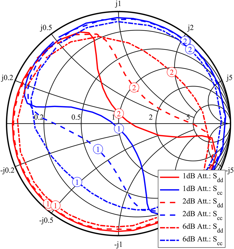
This section shows measurement results of the tuning behavior of the proposed setup using tuners which are connected to each other. Figure 13 shows the impact of a change of attenuation in the connection path. The maximum differential and common mode reflection coefficients which can be achieved with this setup have a magnitude of about 0.94. At the same time, it is possible to set the reflection coefficient of the other mode to a low value. The numbers 1 and 2 in the circles in Fig. 13 indicate specific tuner slide positions, which are used to adjust the phases of a slab line tuner's reflection coefficients. The positions of the slide on each tuner were kept the same. If this were not the case mode, conversion would be generated in the load.

Fig. 13. Impact of attenuator values on the mixed-mode reflection coefficients. The red lines show the change of the common mode reflection coefficient, while the blue lines show the differential mode reflection coefficients. The solid, dashed, and dotted-dashed lines have been captured using different attenuator values in the connection path between the tuners. The circles with the numbers 1 and 2 indicate specific slide positions, which are identical for both tuners. As enforced by (10), both tuners have to use the same settings to prevent mode conversion.
The impact of a phase or delay change in the connection path between the tuners is shown in Fig. 14. As we are only looking at one frequency, a change in delay has the same effect as a phase shift. An increase in delay causes the Smith chart to rotate clockwise. Each extension also introduces some attenuation, changing the magnitude of the mixed-mode reflection coefficients.

Fig. 14. In this plot, the electrical length of the connection path between the tuners was changed. The solid line shows the result for an SMA cable; for the dashed line, the cable was extended with a female–female and male–male adapter. An additional extension was added for the dotted-dashed line. Due to the non-ideal additional insertion loss of each extension also the magnitudes of the reflection coefficients are influenced slightly.
Discussion of measurement results
The maximum achievable reflection coefficients of the proposed setup depend on the chosen attenuation value in the connection path. By comparing Figs 12 and 13, it can be observed that the setup with connected tuners achieves higher magnitude reflection coefficients compared to the setup with directly connected separated tuners. In all presented cases, the maximum achievable reflection coefficients of the proposed setup were higher than what could be reached with traditional setups, while maintaining the possibility to tune the reflection coefficient of the other mode. For example, it can achieve low reflection coefficients for the other mode, similar to the setup with the 180° hybrid shown in Fig. 12. As shown in Fig. 14, the phase of the reflection coefficients can be tuned by adjustment of the delay or phase shift in the transmission path between the tuners. As long as the attenuation in the transmission path is not changed, the magnitudes of the reflection coefficients are not influenced. The disadvantage compared to a setup using a 180° hybrid is that the reflection coefficients cannot be tuned independently, and achieving reflection coefficients in the opposite half of the Smith chart is limited by the minimum attenuation value in the connection path and the transmission coefficients of the tuners. These two factors mainly influence the magnitude of the transmission coefficient of the load network as described in (9)–(12), and this transmission coefficient determines the difference between differential and common mode reflection coefficient. Also not all combinations of differential and common mode reflection coefficients can be generated using the proposed setup. At this point, we would like to remember the reader why it is important for a mixed-mode load-pull system to tune the differential mode and common mode reflection coefficients independently. In real setups, often external baluns are used to convert a differential signal to a single-ended signal. The properties of this balun determine the common mode impedance seen by the DUT, but the differential mode impedance seen by the DUT is mainly determined by the load connected to the single-ended output of the balun. This leads to different common mode and differential mode reflection coefficients being presented to the DUT in a real use case. A good load-pull setup should be able to reproduce these circumstances to properly characterize the DUT.
The analytical results presented in (9)–(12) describe quite well how the setup can be used in practice. Using fixed settings for the tuners, the magnitude of S T can be controlled via the attenuation value in the setup. The lower the attenuation, the higher the magnitude of S T and the larger the difference between differential and common mode reflection coefficients. This behavior is presented in Fig. 13. The phases of the differential and common mode reflection coefficients are directly influenced by the phase of the transmission coefficient. This behavior is represented in Fig. 14.
A drawback of this setup is that the tuning process is more complicated because of the two additional parameters (attenuation and phase) in the connection path. Nevertheless, if the tuning behavior as shown in Figs 13 and 14 is known to the user, also manual tuners can be used in combination with this setup with only a minimum of additional effort. If automatic tuners are available, a pre-characterization of the setup significantly speeds up the tuning process for follow-up measurements. The reader should also keep in mind that this setup does not produce any mode-conversion as long as the two tuners settings are equal. This behavior is the same as it was derived for the setup with directly connected tuners in (3).
Conclusion
Conducting mixed-mode load-pull measurements with a 180° hybrid allows to easily tune differential and common mode load independently of each other, as long as the magnitude and phase imbalance of the hybrid are in an acceptable range. What an “acceptable range” is needs to be defined for each application. To help the reader with this task, a simple formula was derived to estimate the impact of a 180° hybrid imperfection.
Simply connecting tuners directly to the DUT decreases the insertion loss, but forces equal differential and common mode loads. The method proposed by us in [Reference Veit, Gadringer and Leitgeb1] does not need a 180° hybrid, but still allows unequal differential and common mode loads in exchange for ease of use and limited combinations of differential and common mode reflection coefficients. This method also allows to set reflection coefficients of higher magnitude compared to a setup with tuners connected directly to the DUT. An increase of |Γdd,max| from 0.85 to 0.94 was possible using the proposed setup with the same tuners. An increased tuning range can be achieved with the same tuners, by adding an adjustable attenuator and phase shifter in the transmission path between the tuners.
As always, there is not the one best solution. The setup with tuners directly connected to the DUT and matched at the other port has the lowest hardware effort, features higher maximum reflection coefficients than a system using 180° hybrids, but forces equal differential and common mode reflection coefficients. Setups with 180° hybrids allow easy and independent tuning of the individual reflection coefficients, but the hybrid's insertion loss reduces the maximum achievable reflection coefficients. The proposed setup with tuners directly connected to the DUT and also connected to each other via an adjustable attenuator and phase shifter allows even higher reflection coefficients than the setup with directly connected tuners, and the possibility of having different differential and common mode reflection coefficients. But the combinations of different reflection coefficients are more limited compared to the setup using a 180° hybrid, and the hardware effort is the highest of all discussed setups. In the end, the reader has to decide which setup is best suited for each individual application.
Acknowledgement
This work was funded by the Austrian Research Promotion Agency (FFG) under the research project UB-Smart (No.: 859475).
 David Veit received the Dipl.-Ing. degree from Graz University of Technology, Austria, in 2017. Since 2017 he is pursuing his Dr. techn. degree at the Institute of Microwave and Photonic Engineering at Graz University of Technology, Austria. In his studies, he is focusing on RF measurement techniques and UWB system modeling.
 Michael Gadringer received the Dipl.-Ing. and Dr. techn. degrees from Vienna University of Technology, Austria, in 2002 and 2012, respectively. In July 2010, he changed to the Institute of Microwave and Photonic Engineering at Graz University of Technology, Austria. Since 2016, Michael Gadringer has been holding a tenure track research and teaching position at this institute. During his studies, he was involved in the design of analog and digital linearization systems for power amplifiers and in the behavioral modeling of microwave circuits. In his current research activities, he focuses on the design and linearization of broadband microwave and mm-wave communication systems. Additionally, he is involved in planning and implementing complex measurements with an emphasis on calibration and de-embedding techniques. Michael Gadringer has authored 16 journal and 37 conference papers. He fielded four patents and has coedited the book “RF Power Amplifier Behavioral Modeling”, published by Cambridge University Press.
 Erich Leitgeb was born in 1964 in Fürstenfeld (Styria, Austria) and received his master degree at the University of Technology Graz in 1994. In 1994, he started research work in Optical Communications at the Department of Communications and Wave Propagation (TU Graz). In February 1999, he received his Ph.D. degree with honors. Since January 2000, he is the project leader of international research projects in the field of optical communications and he established and leads the research group for Optical Communications at TU Graz. End of 2003 he submitted his research work for the Associate Professor. Since 2011, he is a Professor for Optical Communications and Wireless Applications at the Institute of Microwave and Photonic Engineering at TU Graz. Erich Leitgeb is the author and co-author of five book-chapters, around 40 journal publications, 140 reviewed conference papers, around 40 invited talks, and more than 60 international scientific reports.


 Open access