


1. Introduction
Homeownership rates differ widely across developed countries. Within the Euro Area, Germany has the lowest homeownership rate with only 43% of households owning their main residence, whereas in Italy the fraction of homeowners is much higher at 68%, and in Spain even exceeds 83%. These persistent cross-country differences have sparked a large body of research exploring the determinants of the choice between owning and renting. In this paper, we present evidence that co-residence, that is, living in the parental household, is an important decision to explain this gap—a mechanism, which most of the previous literature has largely overlooked.
Throughout, we focus attention on a comparison of two countries that exhibit particularly striking differences in living arrangements, which put them at the center of the public debate on low versus high homeownership rates—Germany (low) and Italy (high). We argue that accounting for co-residence is key for understanding homeownership rates for three reasons. First, we show that the fraction of people co-residing with their parents differs significantly across countries. In Germany, roughly 27% of young adults aged 17–40 years co-reside with their parents, while Italy has one of the highest co-residence rates among European countries with a value that is more than twice as high at 61%.Footnote 1 Second, we argue that these differences manifest themselves in differences in the homeownership rate, the reason being that the latter is conventionally measured on the household level, not the individual level.Footnote 2 Comparing again Germany and Italy, we show that for young adults the gap in homeownership rates disappears entirely once co-residing individuals who do not form their own household are correctly accounted for. Third, and most importantly, we argue that the choice between owning, renting and co-residing is intrinsically intertwined and should be studied jointly. In light of this three-way trade-off, we ask two main research questions: What are the determinants of the preferred living arrangement along the life cycle? And to what extent do economic factors, housing policies, and preferences explain cross-country differences in co-residence patterns and housing choices?
To answer these questions, we build a novel incomplete markets overlapping-generations equilibrium model with an intergenerational link between children and their parents, which allows us to embed co-residence as a third form of living arrangement next to owning and renting. Model agents who choose to live with their parents do not have to pay rent, at the expense of incurring a utility loss from the lack of independence. Housing services are provided by the parents and shared among all household members. Importantly, parents take the economic circumstances and decisions of their children—that is, their income position, financial assets, housing wealth, and their co-residence decision—into account, and vice versa. This gives rise to a rich set of dynamics between family members and is a key contribution of our model. On the aggregate, house prices and rents are determined in equilibrium and depend on a supply technology with diminishing returns in the construction sector.
We calibrate the model to the German economy, taking as inputs the age-dependent individual income process as estimated from the German Socio-Economic Panel (SOEP) as well as housing policy parameters describing the institutional features of the German housing market. The calibrated model matches well key features of the data, such as the age profiles of homeownership and co-residence, and the accumulation patterns of wealth and its components over the life cycle. We then use the model to explore the determinants of these patterns in a series of counterfactual experiments, focusing on Germany and Italy.
Our main results are as follows. First, when replacing the German income process by its Italian counterpart, we find that more individuals choose to co-reside, especially among the young. The intuition is that Italian wages tend to be lower and increase later in life. This induces more people to postpone moving out of the parental household and renting their own apartment. Second, we explore the role of housing policy: Germany is known to have relatively well-functioning rental markets, an extensive social housing sector, and other policies and institutions favoring renters. Against this backdrop, we conduct a stylized experiment where we lower the price-rent ratio, that is, the relative price of owning versus renting, to match the Italian homeownership rate. Our simulations indicate a substantial drop in the share of renting households, while at the same time leaving the share of co-residents almost unchanged. Finally, we show that differential preferences for living in a multigenerational household can explain the remaining gap in co-residence patterns. With a weaker taste for independence, the model generates life-cycle profiles for homeownership, rented housing and co-residence that closely resemble the observed patterns in Italy.
Our paper contributes to the burgeoning literature on housing in macroeconomics, surveyed in Davis and van Nieuwerburgh (Reference Davis and van Nieuwerburgh2015) and Piazzesi and Schneider (Reference Piazzesi and Schneider2016). To our knowledge, our paper is the first to include co-residence as a living arrangement, next to owning and renting, into a quantitative macroeconomic model, which we show to be a very important margin. A large strand of research has focused on understanding the age profile of homeownership. Some of these papers emphasize the importance of collateral and borrowing constraints for explaining the steep initial increase and the flattening out toward retirement (Ortalo-Magne and Rady (Reference Ortalo-Magne and Rady2006), Yang (Reference Yang2009), Fernández-Villaverde and Krueger (Reference Fernández-Villaverde and Krueger2011), Goodman and Mayer (Reference Goodman and Mayer2018)). Our paper contributes to this line of research by introducing a novel link between housing tenure choices and co-residence decisions and by illustrating the difference between homeownership rates measured at the individual and at the household level. Yao and Zhang (Reference Yao and Zhang2005) argue that the possibility to rent is particularly important for young and poor households who cannot afford the downpayment on a house. Our paper adds to this notion by embedding the co-residence channel as an informal substitute for renting.
The structural model in our paper builds on the framework developed by Kaas et al. (Reference Kaas, Kocharkov, Preugschat and Siassi2021). Exploring potential reasons behind Germany’s low homeownership rate, these authors find that taxes and social housing can account for roughly two thirds of the gap in homeownership to the United States. Our framework simplifies their model along some dimensions—for example, we abstract from house price and rental rate risk—, but explicitly adds an intergenerational link between parents and children, and an endogenous household formation decision. In terms of modeling distortions in the market for rental housing, our paper is closely related to Kindermann and Kohls (Reference Kindermann and Kohls2018). These authors develop a general equilibrium life-cycle model to study the negative relation between homeownership and wealth inequality across European countries, and they show that differences in rental market inefficiencies can explain about half of this variation.
Our paper further relates to a strand of literature that tries to quantify the effects of tax policy on homeownership. Many papers focus on the effects of mortgage interest deductibility, for example, Gervais (Reference Gervais2002), Chambers et al. (Reference Chambers, Garriga and Schlagenhauf2009), Sommer and Sullivan (Reference Sommer and Sullivan2018) and Floetotto et al. (Reference Floetotto, Kirker and Stroebel2016). Yang (Reference Yang2009) highlights the importance of transaction costs for matching the slow downsizing of housing wealth toward the end of the life cycle. On the institutional side, Andrews et al. (Reference Andrews, Sanchez and Johansson2011) shed light on the regulatory differences in the housing market in OECD and Euro Area countries.
Finally, our paper relates to a growing literature that moves beyond the stand-in household assumption and integrates families explicitly into macroeconomic models (Doepke and Tertilt (Reference Doepke and Tertilt2016) and Greenwood et al. (Reference Greenwood, Guner and Vandenbroucke2017) provide recent surveys). An important theme in this literature is insurance within the family, for example, between young and old family members. For instance, Kaplan (Reference Kaplan2012) studies a model where children have the option to co-reside with their parents as a device to smooth out income shocks. Compared to our model, in his setting parents are not allowed to save, and he does not consider the choice between renting and owning. Barczyk and Kredler (Reference Barczyk and Kredler2018) use an overlapping-generations model with imperfectly altruistic generations to model long-term care decisions of families highlighting the importance of informal care. Informal care provision may be an important reason for co-residence potentially adding to the channels we look at in our work.
The remainder of the paper is organized as follows. Section 2 presents empirical facts on homeownership rates and co-residence patterns, with a special focus on Germany and Italy. Section 3 describes the structural model. After calibrating the model to Germany, we evaluate its fit to the data and explore the dynamics of co-residence in Section 4. Then we conduct our main counterfactual experiments in Section 5. Some concluding remarks are contained in Section 6.
2. Empirical facts
In this section, we document some stylized facts on homeownership and co-residence patterns across European countries. Our main data source is the Household Finance and Consumption Survey (HFCS). This is a well-known harmonized micro data survey that is administered by the European Central Bank. Our analysis is based on the second wave of the HFCS which was collected in 2014, and we restrict our sample to the ten largest Euro Area countries. Even though our presentation can be interpreted in general terms, much of it will be focused on Germany and Italy.
Fig. 1 presents homeownership rates across the countries in our sample. As is standard practice in the literature, we define homeowning households to be households that own at least part of their main residence. Fig. 1 shows that there are massive cross-country differences in the homeownership rate: In Germany, only about 43% of households are homeowners, almost 25 percentage points lower than in Italy where the homeownership rate is roughly 68%.

Figure 1. Homeownership rates across euro area countries.
Notes: Homeownership rates at the household level.
Source: Own calculations based on HFCS (second wave, 2014).
We next show that part of this difference can be traced back to the fact that homeownership is conventionally measured at the household level, and not the individual level. It will become clear that this distinction becomes relevant when some individuals decide not to form their own households (and become owners or renters), but instead choose to co-reside with their parents or grandparents. We define an individual to be co-residing if her/his (grand-)parents are living in the same household and one of them is classified as the head of household.Footnote 3 If the household is not headed by a (grand-)parent, then the individual is either classified as an owner or a renter.Footnote 4
Fig. 2 provides a visual description of the life-cycle patterns of owning, renting, and co-residing in Germany and Italy showing that co-residence constitutes an empirically relevant choice of living arrangement in both countries, in particular among young adults. In Germany, roughly 60% of individuals between 17 and 24 co-reside with their parents or grandparents. Among those aged 25–32 years, the share is already considerably lower at 18%, and it then quickly drops to negligible values for older ages. In Italy, co-residence also exhibits a monotonically declining life-cycle pattern, albeit at much higher values. For instance, the share of 17–24-year-olds living in their parents’ household is close to 95%. Among those aged 25–32 years, where most of them have completed their education and started their professional career, the share of those co-residing still exceeds 60%. Even in higher age groups, there is a significant share of people who choose to co-reside with their parents. Regarding the other two forms of living arrangement, a well-known pattern appears: young individuals are more likely to be renters, and the homeownership rate then increases over the life cycle.
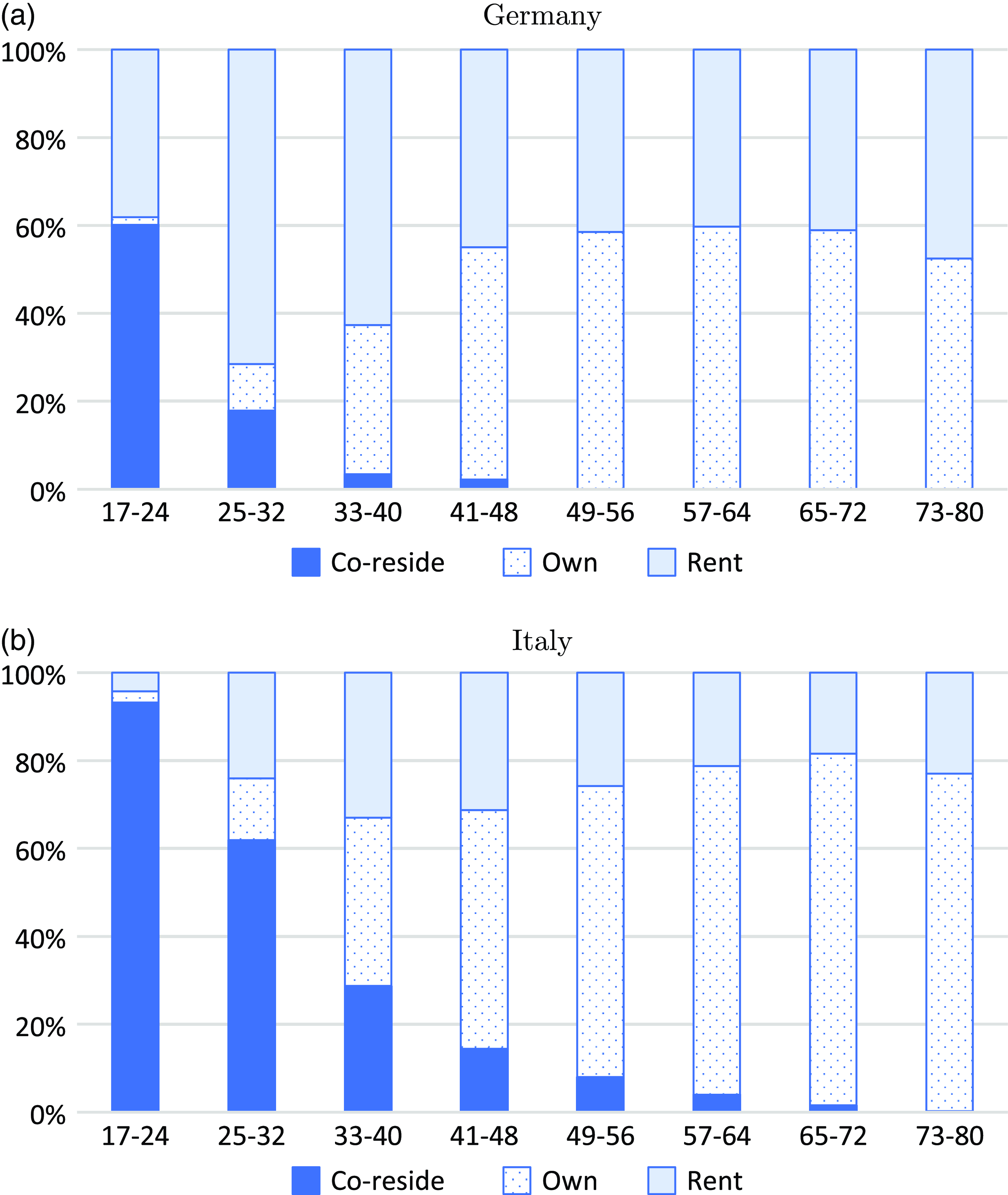
Figure 2. Split of living arrangements over the life cycle: Germany and Italy.
Source: Own calculations based on HFCS (second wave, 2014). The figure shows the split of living arrangements in (a) Germany and (b) Italy. Calculations are based on the individual as the unit of measurement.
Next, we illustrate why this disparity in homeownership is partially related to the fact that some people choose to co-reside in their parental household. Fig. 3 plots the homeownership rates over the life cycle in Germany and Italy. The left panel employs the conventional approach of basing the homeownership on the household being the unit of observation. By contrast, the right panel measures homeownership rates based on individuals, that is, it shows the actual fraction of people owning their main residence for each age group. Assuming the perspective of the household as the relevant unit of observation (left panel) suggests a significantly higher homeownership rate across all age groups in Italy than in Germany. Does this mean that Italians are much more likely to be owner-occupiers than Germans, at any point of the life cycle? The answer is no. During the first part of the adult life cycle, many of them co-reside with their (grand-)parents and thus do not constitute a household. In fact, the individual ownership profiles in Germany and Italy are barely distinguishable until the age of 48 and only then start to spread out.

Figure 3. Homeownership over the life cycle: Germany and Italy.
Notes: The figure shows the share of homeowners in Germany (continuous line) and Italy (dashed line). The left panel takes as measurement unit the age of the household head. The right panel takes the age of the individual. Source: Own calculations based on HFCS (second wave, 2014).
An important conclusion is that to understand cross-country differences in homeownership rates it is necessary to account for differences in co-residence patterns. This is particularly true for young individuals, leading us to the question: What determines their choice to live with their parents or grandparents? Next to preferences and cultural factors, income and affordability of rental, respectively owned, housing are prime economic factors that can be relevant when individuals make the decision to co-reside. Fig. 4 suggests that the choice of living arrangement may indeed be related to income levels. In this figure, we plot average income by age and living arrangement from the data for Germany. Conditional on age, income-poor individuals are much more likely to be living in the parental household. This is particularly true among the first two age groups, which is when co-residence is more prevalent than later in life.Footnote 5 This points to co-residence as an informal substitute for formal rental housing when income is low. In a similar vein, the affordability of rental housing might play an important role as well: In well-functioning rental markets, a lower relative price of rental housing versus owner-occupied housing might induce more individuals to become renters. The efficiency of rental housing markets is itself determined by government-mandated housing policies (subsidized social housing, taxation, etc.) as well as the legal regulatory framework. However, it is difficult to identify empirically the contribution of well-functioning rental markets in shaping co-residence and homeownership patterns. Therefore, we now turn to laying out our structural model.

Figure 4. Average income by living arrangement in Germany.
Source: Own calculations based on HFCS (second wave, 2014). Income values have been rescaled to account for variations in household size beyond co-residence (see caption to Fig. 8 for details).
3. A life-cycle model of co-residing, renting and owning
We consider an overlapping-generations economy that is populated by households, firms, and the government. The model features a housing market where house prices and rental rates are determined endogenously, while wage processes and the safe real interest rate are taken as exogenous. Time is discrete and a period in the model corresponds to one year. We consider a stationary equilibrium where prices and distribution measures are constant over time.
3.1 Households
Agents. Throughout the paper, we use the term “agent” to refer to the main economic decision unit in our model. This decision unit can be thought of as representing a generation, where age-specific variations in its size (e.g., getting married and/or having kids) are not explicitly modeled and taken as exogenous. As described below, we introduce equivalence scales in order to capture variations in the size of the decision unit, beyond co-residence.
Demographics. The household model is cast at an annual frequency. We denote by $j = \{1,\ldots,J=65\}$
the age of an agent in our model. Agents enter the economy at model age
$j = \{1,\ldots,J=65\}$
the age of an agent in our model. Agents enter the economy at model age $j = 1$
, which corresponds to the biological age of 17 years, and survive with certainty in each model period until they die with certainty at the end of age
$j = 1$
, which corresponds to the biological age of 17 years, and survive with certainty in each model period until they die with certainty at the end of age $J$
. Each agent is part of a dynasty where successive generations of parents and children are born 30 years apart. Agents live through three life-cycle stages. During the first 30 years of their lives (first stage), each period, an agent has the option to co-reside with her/his parents, in which case multiple members of the family live in the same dwelling. Through this mechanism, the number and the composition of households in the model economy is determined endogenously. If an agent chooses to own or rent a housing unit instead, s/he forms her own household. At model age
$J$
. Each agent is part of a dynasty where successive generations of parents and children are born 30 years apart. Agents live through three life-cycle stages. During the first 30 years of their lives (first stage), each period, an agent has the option to co-reside with her/his parents, in which case multiple members of the family live in the same dwelling. Through this mechanism, the number and the composition of households in the model economy is determined endogenously. If an agent chooses to own or rent a housing unit instead, s/he forms her own household. At model age $31$
(second stage), the agent becomes part of the parent generation and is now linked to her/his own children, which are born into the economy at age 31. Since the measure of newborns is the same as the measure of parents, the population size is constant and normalized to unity. At model age
$31$
(second stage), the agent becomes part of the parent generation and is now linked to her/his own children, which are born into the economy at age 31. Since the measure of newborns is the same as the measure of parents, the population size is constant and normalized to unity. At model age $61$
, the agent becomes part of the grandparent generation (third stage). Overlaying these life-cycle stages are two life-cycle phases, a working phase spanning the model ages
$61$
, the agent becomes part of the grandparent generation (third stage). Overlaying these life-cycle stages are two life-cycle phases, a working phase spanning the model ages $j \in \{1,\ldots,j_r=48\}$
and a retirement phase for all model ages
$j \in \{1,\ldots,j_r=48\}$
and a retirement phase for all model ages $j \in \{j_r+1=49,\ldots,J=65\}$
. Fig. 5 gives a stylized representation of the time line of the overlapping generations model by showing the life cycles of three overlapping generations, labeled as “parents,” “children,” and “grandchildren.”
$j \in \{j_r+1=49,\ldots,J=65\}$
. Fig. 5 gives a stylized representation of the time line of the overlapping generations model by showing the life cycles of three overlapping generations, labeled as “parents,” “children,” and “grandchildren.”

Figure 5. Life cycle of parents, children and grandchildren.
Notes: Stylized representation of three overlapping generations (parents, children, and grandchildren).
Preferences and co-residence. Agents maximize expected lifetime utility with time discount factor $\beta$
and period utility
$\beta$
and period utility $U \big (c,\hat{s},x;j,\unicode{x1D7D9}_{h \gt 0})$
, where
$U \big (c,\hat{s},x;j,\unicode{x1D7D9}_{h \gt 0})$
, where $c$
denotes consumption of nonhousing goods,
$c$
denotes consumption of nonhousing goods, $\hat{s}$
is consumption of housing services, and
$\hat{s}$
is consumption of housing services, and $x \in \{0,1\}$
is an indicator variable for co-residence. We assume that housing services are provided by the parents and shared by all co-residing members of the family. Co-residence affects agents in two ways. First, due to the sharing of resources, per-capita consumption of housing services
$x \in \{0,1\}$
is an indicator variable for co-residence. We assume that housing services are provided by the parents and shared by all co-residing members of the family. Co-residence affects agents in two ways. First, due to the sharing of resources, per-capita consumption of housing services $\hat{s}$
differs from overall housing services purchased by the household,
$\hat{s}$
differs from overall housing services purchased by the household, $s$
. Specifically, we will use household equivalence scales that depend on co-residence choices.Footnote 6 Second, for children we will embed an age-dependent utility cost from co-residing with one’s parents, capturing the desire for independence. Following Kaas et al. (Reference Kaas, Kocharkov, Preugschat and Siassi2021), we further include an additional utility gain for retired homeowners, reflecting the notion that retirees may enjoy own housing more than rented housing. When parameterizing our utility function, this utility shifter will only apply to retired agents (
$s$
. Specifically, we will use household equivalence scales that depend on co-residence choices.Footnote 6 Second, for children we will embed an age-dependent utility cost from co-residing with one’s parents, capturing the desire for independence. Following Kaas et al. (Reference Kaas, Kocharkov, Preugschat and Siassi2021), we further include an additional utility gain for retired homeowners, reflecting the notion that retirees may enjoy own housing more than rented housing. When parameterizing our utility function, this utility shifter will only apply to retired agents ( $j\gt j_r$
) who own
$j\gt j_r$
) who own $h \gt 0$
housing units.Footnote 7
$h \gt 0$
housing units.Footnote 7
Labor and pension income. Gross labor income during working age consists of an age-dependent, deterministic component $\varepsilon (j)$
, and a residual random component
$\varepsilon (j)$
, and a residual random component $\eta (j) \in E(j) = \left [\underline{\eta }_j,\ldots,\overline{\eta }_j\right ]^\prime$
,
$\eta (j) \in E(j) = \left [\underline{\eta }_j,\ldots,\overline{\eta }_j\right ]^\prime$
,
 \begin{equation} \ln y(\eta,j) = \varepsilon (j) + \eta (j). \end{equation}
The residual income component $\eta (j)$
evolves according to a Markov chain with age-dependent transition matrix
$\eta (j)$
evolves according to a Markov chain with age-dependent transition matrix $\pi \left (\eta (j+1) \mid \eta (j); j\right )$
and age
$\pi \left (\eta (j+1) \mid \eta (j); j\right )$
and age $j$
specific stationary invariant distribution
$j$
specific stationary invariant distribution $\Pi (\eta ;j)$
. Retired agents receive nonstochastic and constant pension benefits. We assume that retirement benefits are a function of the last realization of the income shock prior to retirement,
$\Pi (\eta ;j)$
. Retired agents receive nonstochastic and constant pension benefits. We assume that retirement benefits are a function of the last realization of the income shock prior to retirement, $\eta (j_r)$
, partially reflecting the fact that higher earnings lead to higher pension income.Footnote 8
$\eta (j_r)$
, partially reflecting the fact that higher earnings lead to higher pension income.Footnote 8
3.2 Assets
Housing. Housing units $h$
can be owned by private agents and rental firms. Houses are restricted to the ordered set of discrete sizes
$h$
can be owned by private agents and rental firms. Houses are restricted to the ordered set of discrete sizes $\mathcal{H} \in \{\underline{h},\ldots,\bar{h}\}$
, and they are traded at unit price
$\mathcal{H} \in \{\underline{h},\ldots,\bar{h}\}$
, and they are traded at unit price $p$
at the end of the period. One unit of housing provides one unit of shelter. A homeowning agent (
$p$
at the end of the period. One unit of housing provides one unit of shelter. A homeowning agent ( $h \gt 0$
) obtains
$h \gt 0$
) obtains $s = h$
units of housing services. Renting agents (
$s = h$
units of housing services. Renting agents ( $h = 0$
) buy housing services
$h = 0$
) buy housing services $s$
at price
$s$
at price $\rho$
on the rental market. In every period, the housing stock depreciates at rate
$\rho$
on the rental market. In every period, the housing stock depreciates at rate $\delta$
. As in İmrohoroğlu et al. (Reference Imrohoroğlu, Matoba and Tüzel2018) and outlined in Piazzesi and Schneider (Reference Piazzesi and Schneider2016), we assume that homeowners have to pay this fraction of their home value which make it conceptually similar to maintenance costs. When an agent buys or sells housing units, s/he incurs transaction costs, which are fractions
$\delta$
. As in İmrohoroğlu et al. (Reference Imrohoroğlu, Matoba and Tüzel2018) and outlined in Piazzesi and Schneider (Reference Piazzesi and Schneider2016), we assume that homeowners have to pay this fraction of their home value which make it conceptually similar to maintenance costs. When an agent buys or sells housing units, s/he incurs transaction costs, which are fractions $t^b$
(buyer) and
$t^b$
(buyer) and $t^s$
(seller) of the house price:
$t^s$
(seller) of the house price:
 \begin{equation} \gamma (h,h^{\prime }) = \begin{cases} t^s p h + t^b p h^{\prime }, & \text{if}\; h \ne h^\prime, \\ 0 & \text{else}. \end{cases} \end{equation}
Financial assets. Agents can save in a risk-free bond at interest rate $r$
, and they can borrow against their houses at mortgage rate
$r$
, and they can borrow against their houses at mortgage rate $r+\iota ^m$
,
$r+\iota ^m$
, $\iota ^m\gt 0$
. The mortgage premium
$\iota ^m\gt 0$
. The mortgage premium $\iota ^m$
is exogenous, potentially reflecting monitoring and administrative costs of mortgage lenders. Let
$\iota ^m$
is exogenous, potentially reflecting monitoring and administrative costs of mortgage lenders. Let $a$
denote an agent’s net financial assets. Newborn agents hold zero assets. Mortgage borrowing is subject to a downpayment constraint,
$a$
denote an agent’s net financial assets. Newborn agents hold zero assets. Mortgage borrowing is subject to a downpayment constraint,
 \begin{equation} a' \geq -p (1-\theta _j) h', \end{equation}
where $\theta _j$
is an age-specific downpayment parameter, and
$\theta _j$
is an age-specific downpayment parameter, and $a'$
and
$a'$
and $h'$
denote the agent’s choice for next period’s net financial assets and housing assets.
$h'$
denote the agent’s choice for next period’s net financial assets and housing assets.
3.3 Recursive formulation of the decision problems
Our model features intergenerational links between parents and their children, which implies that both groups have to take into account the respective state variables of the other age group. The state vector of an agent is $(a,h,\eta,\tilde{a},\tilde{h},\tilde{\eta },j)$
, where the first three components
$(a,h,\eta,\tilde{a},\tilde{h},\tilde{\eta },j)$
, where the first three components $(a,h,\eta )$
summarize her/his own net financial assets, housing assets, and residual income. If
$(a,h,\eta )$
summarize her/his own net financial assets, housing assets, and residual income. If $j \leq 30$
, the next three components
$j \leq 30$
, the next three components $(\tilde{a},\tilde{h},\tilde{\eta })$
reflect the state variables of the parents; if
$(\tilde{a},\tilde{h},\tilde{\eta })$
reflect the state variables of the parents; if $30 \lt j \leq 60$
, they denote the state variables of the children; if
$30 \lt j \leq 60$
, they denote the state variables of the children; if $j \geq 61$
, for brevity of notation, we simply set
$j \geq 61$
, for brevity of notation, we simply set $(\tilde{a},\tilde{h},\tilde{\eta }) = (\emptyset,\emptyset,\emptyset )$
. Note that due to the fixed age difference between subsequent generations,
$(\tilde{a},\tilde{h},\tilde{\eta }) = (\emptyset,\emptyset,\emptyset )$
. Note that due to the fixed age difference between subsequent generations, $j$
determines the age of the other group
$j$
determines the age of the other group $\tilde{j}$
as well:
$\tilde{j}$
as well: $\tilde{j} = j + 30$
if
$\tilde{j} = j + 30$
if $j \leq 30$
, and
$j \leq 30$
, and $\tilde{j} = j - 30\;$
if
$\tilde{j} = j - 30\;$
if $j \gt 30$
.
$j \gt 30$
.
Let $V(a,h,\eta,\tilde{a},\tilde{h},\tilde{\eta },j)$
denote an agent’s value function. Agents choose consumption of nonhousing goods
$V(a,h,\eta,\tilde{a},\tilde{h},\tilde{\eta },j)$
denote an agent’s value function. Agents choose consumption of nonhousing goods $c$
, housing services
$c$
, housing services $s$
(unless they are co-residing in which case this will be chosen by their parents), financial assets
$s$
(unless they are co-residing in which case this will be chosen by their parents), financial assets $a'$
, and housing assets
$a'$
, and housing assets $h'$
for next period. During the first 30 years, they also choose whether to co-reside with their parents
$h'$
for next period. During the first 30 years, they also choose whether to co-reside with their parents $x$
. We denote the policy functions by
$x$
. We denote the policy functions by $C(\!\cdot\!)$
for consumption, by
$C(\!\cdot\!)$
for consumption, by $S(\!\cdot\!)$
for housing services, by
$S(\!\cdot\!)$
for housing services, by $A(\!\cdot\!)$
and
$A(\!\cdot\!)$
and $H(\!\cdot\!)$
for financial and housing assets, and by
$H(\!\cdot\!)$
for financial and housing assets, and by $X(\!\cdot\!)$
for co-residence. Thus, for example,
$X(\!\cdot\!)$
for co-residence. Thus, for example, $X(a,h,\eta,\tilde{a},\tilde{h},\tilde{\eta },j)=1$
means that an agent of age
$X(a,h,\eta,\tilde{a},\tilde{h},\tilde{\eta },j)=1$
means that an agent of age $j$
with own state variables
$j$
with own state variables $(a,h,\eta )$
chooses to co-reside with its parents of age
$(a,h,\eta )$
chooses to co-reside with its parents of age $j+30$
with state variables
$j+30$
with state variables $(\tilde{a},\tilde{h},\tilde{\eta })$
, and
$(\tilde{a},\tilde{h},\tilde{\eta })$
, and $X(\tilde{a},\tilde{h},\tilde{\eta },a,h,\eta,\tilde{j})=1$
means that an agent of age
$X(\tilde{a},\tilde{h},\tilde{\eta },a,h,\eta,\tilde{j})=1$
means that an agent of age $\tilde{j}+30$
with own state variables
$\tilde{j}+30$
with own state variables $(a,h,\eta )$
has co-residing children of age
$(a,h,\eta )$
has co-residing children of age $\tilde{j}$
and state variables
$\tilde{j}$
and state variables $(\tilde{a},\tilde{h},\tilde{\eta })$
.
$(\tilde{a},\tilde{h},\tilde{\eta })$
.
Housing decision. The discrete choice problem between owning and not owning can be concisely described as
 \begin{equation} V(a,\eta,\tilde{a},\tilde{h},\tilde{\eta },j) \:=\: \max _{h \in \{0,\mathcal{H}\}} \Big \{ V(a,h,\eta,\tilde{a},\tilde{h},\tilde{\eta },j) \Big \}. \end{equation}
Note that this formulation accommodates both the possibility of not becoming a homeowner at all ( $h = 0$
) and choosing from the menu of the various discrete house sizes conditional on becoming a homeowner (
$h = 0$
) and choosing from the menu of the various discrete house sizes conditional on becoming a homeowner ( $h \gt 0$
).
$h \gt 0$
).
Homeowners. Let $V(a,h\gt 0,\eta,\tilde{a},\tilde{h},\tilde{\eta },j)$
denote the value function of an agent who currently owns a house of some size
$V(a,h\gt 0,\eta,\tilde{a},\tilde{h},\tilde{\eta },j)$
denote the value function of an agent who currently owns a house of some size $h \in \mathcal{H}$
. This agent solves the recursive problem
$h \in \mathcal{H}$
. This agent solves the recursive problem
 \begin{equation} V(a,h\gt 0,\eta,\tilde{a},\tilde{h},\tilde{\eta },j) \;=\; \max _{c,a',h'} U \big (c,\hat{s},0;j,1) + \beta \mathbb{E}_{\eta ^\prime,\tilde{\eta }^\prime \mid \eta, \tilde{\eta }, j} \left [V(a^{\prime },\eta ^{\prime },\tilde{a}^{\prime },\tilde{h}^{\prime },\tilde{\eta }^{\prime },j+1)\right ] \end{equation}
subject to
 \begin{align} c + a' + p h' + \delta p h + \gamma (h,h') \;&=\; y(\eta,j) - T_j(\bar{y}) + p h + \big [ 1 + r \unicode{x1D7D9}_{a \gt 0} + (r+\iota ^m) \unicode{x1D7D9}_{a \lt 0} \big ] a, \end{align}
 \begin{align} \bar{y} \;&=\; y(\eta,j) + r \max (a,0), \end{align}
 \begin{align} a' \;&\geq \; -p (1-\theta _j) h', \text{and} h' \in \mathcal{H} \cup \{0\}, \end{align}
 \begin{align} \hat{s} \;&=\; h/n(X(\tilde{a},\tilde{h},\tilde{\eta },a,h,\eta,\tilde{j}),j) \end{align}
 \begin{align} \tilde{a}^{\prime } \;&=\; A(\tilde{a},\tilde{h},\tilde{\eta },a,h,\eta,\tilde{j}), \end{align}
 \begin{align} \tilde{h}^{\prime } \;&=\; H(\tilde{a},\tilde{h},\tilde{\eta },a,h,\eta,\tilde{j}). \end{align}
Equation (6a) is the budget constraint, which states that expenditures on consumption, financial and housing assets, maintenance costs, and transaction costs for buying/selling must be equal to the sum of labor (or pension) income net of taxes, and financial and housing assets. Taxes are a function $T_j(\bar{y})$
of the tax base
$T_j(\bar{y})$
of the tax base $\bar{y}$
, which is defined in equation (6b) as the sum of labor and asset income. For simplicity, we assume that during retirement income is not taxed. Equation (6c) is the borrowing constraint. Equation (6d) maps overall housing services into per-capita consumption of housing services by using equivalence weights, denoted by
$\bar{y}$
, which is defined in equation (6b) as the sum of labor and asset income. For simplicity, we assume that during retirement income is not taxed. Equation (6c) is the borrowing constraint. Equation (6d) maps overall housing services into per-capita consumption of housing services by using equivalence weights, denoted by $n(x,j)$
, for households that have co-residents (
$n(x,j)$
, for households that have co-residents ( $n(x=1,j)$
) and those that do not (
$n(x=1,j)$
) and those that do not ( $n(x=0,j)$
). Equations (6e) and (6f) define the laws of motion for financial and housing assets by the parents/children, respectively, as described by their policy functions.
$n(x=0,j)$
). Equations (6e) and (6f) define the laws of motion for financial and housing assets by the parents/children, respectively, as described by their policy functions.
None-homeowners. Next, denote by $V(a,h=0,\eta,\tilde{a},\tilde{h},\tilde{\eta },j)$
the value function of an agent who currently does not own a house. This agent can choose housing services
$V(a,h=0,\eta,\tilde{a},\tilde{h},\tilde{\eta },j)$
the value function of an agent who currently does not own a house. This agent can choose housing services $s$
on the rental market. If the agent is of age
$s$
on the rental market. If the agent is of age $j \leq 30$
, s/he also has the alternative option of co-residing with her/his parents. The recursive problem reads as follows:
$j \leq 30$
, s/he also has the alternative option of co-residing with her/his parents. The recursive problem reads as follows:
 \begin{equation} V(a,h=0,\eta,\tilde{a},\tilde{h},\tilde{\eta },j) \;=\; \max _{c,s,x,a',h'} U \big (c,\hat{s},x;j,0) + \beta \mathbb{E}_{\eta ^\prime,\tilde{\eta }^\prime \mid \eta, \tilde{\eta }, j} \left [V(a^{\prime },\eta ^{\prime },\tilde{a}^{\prime },\tilde{h}^{\prime },\tilde{\eta }^{\prime },j+1) \right ] \end{equation}
subject to
 \begin{align} c + a' + p h' + \gamma (0,h') \;&=\; y(\eta,j) - T_j(\bar{y}) - \unicode{x1D7D9}_{x = 0} \rho s + \big [ 1 + r \unicode{x1D7D9}_{a \gt 0} + (r+\iota ^m) \unicode{x1D7D9}_{a \lt 0} \big ] a, \end{align}
 \begin{align} \bar{y} \;&=\; y(\eta,j) + r \max (a,0), \end{align}
 \begin{align} a' \;&\geq \; -p (1-\theta _j) h', \text{and} h' \in \mathcal{H} \cup \{0\}, \end{align}
 \begin{align} \hat{s} \;&=\; \begin{cases} S(\tilde{a},\tilde{h},\tilde{\eta },a,0,\eta,\tilde{j})/n(x=1,j) & \:\text{if}\: x = 1, \\ s/n(X(\tilde{a},\tilde{h},\tilde{\eta },a,h,\eta,\tilde{j}),j) & \text{ otherwise}, \end{cases} \end{align}
 \begin{align} x \in \{0,1\} & \:\text{ if }\: j \leq 30, \;\text{and } x = 0 \text{ otherwise}, \end{align}
 \begin{align} \tilde{a}^{\prime } \;&=\; A(\tilde{a},\tilde{h},\tilde{\eta },a,h,\eta,\tilde{j}), \end{align}
 \begin{align} \tilde{h}^{\prime } \;&=\; H(\tilde{a},\tilde{h},\tilde{\eta },a,h,\eta,\tilde{j}). \end{align}
The distinction between renting and co-residing is reflected in equation (8d), where $S(\!\cdot\!)$
denotes the policy function for housing services. Note that
$S(\!\cdot\!)$
denotes the policy function for housing services. Note that $S(\tilde{a},\tilde{h},\tilde{\eta },a,0,\eta,\tilde{j})$
describes the housing services that are chosen by the parents. Thus, if
$S(\tilde{a},\tilde{h},\tilde{\eta },a,0,\eta,\tilde{j})$
describes the housing services that are chosen by the parents. Thus, if $j \leq 30$
and
$j \leq 30$
and $x=1$
, then
$x=1$
, then $S(\tilde{a},\tilde{h},\tilde{\eta },a,0,\eta,\tilde{j})/n(x=1,j)$
is the housing service flow utility that a child of age
$S(\tilde{a},\tilde{h},\tilde{\eta },a,0,\eta,\tilde{j})/n(x=1,j)$
is the housing service flow utility that a child of age $j$
experiences from co-residing with its parents. The second line in equation (8d) reflects the case where the agent is a renter, in which case the housing service flow depends on whether there are co-residents,
$j$
experiences from co-residing with its parents. The second line in equation (8d) reflects the case where the agent is a renter, in which case the housing service flow depends on whether there are co-residents, $n(x=1,j)$
, or not,
$n(x=1,j)$
, or not, $n(x=0,j)$
. If the agent chooses to rent (
$n(x=0,j)$
. If the agent chooses to rent ( $x = 0$
), s/he can choose
$x = 0$
), s/he can choose $s$
freely, but has to pay expenditures on rent as reflected in the budget constraint (8a). Equation (8e) imposes an age restriction on the option of co-residing, and equations (8f) and (8g) mirror those from an owner’s problem above.
$s$
freely, but has to pay expenditures on rent as reflected in the budget constraint (8a). Equation (8e) imposes an age restriction on the option of co-residing, and equations (8f) and (8g) mirror those from an owner’s problem above.
3.4 Rental firms and construction sector
We follow Kaas et al. (Reference Kaas, Kocharkov, Preugschat and Siassi2021) in their modeling of the real-estate market and assume that rental firms need to pay monitoring costs $\mu$
per unit of rented housing. These costs reflect the information asymmetry between a real-estate firm and its renters, and they create a wedge between prices and rents that imply a motive for homeownership. The market of real-estate firms is competitive. As a result, the zero-profit condition implies that house prices and rental rates are related as
$\mu$
per unit of rented housing. These costs reflect the information asymmetry between a real-estate firm and its renters, and they create a wedge between prices and rents that imply a motive for homeownership. The market of real-estate firms is competitive. As a result, the zero-profit condition implies that house prices and rental rates are related as
 \begin{equation} (r + \delta ) p = \rho - \mu. \end{equation}
There is a construction sector producing housing units. Production entails costs which are convex and increasing in housing units, $K(I)$
with
$K(I)$
with $K^\prime (I) \gt 0$
, and
$K^\prime (I) \gt 0$
, and $K^{\prime \prime }(I) \gt 0$
. The maximization problem of the construction sector implies
$K^{\prime \prime }(I) \gt 0$
. The maximization problem of the construction sector implies
 \begin{equation} p = K^\prime (I). \end{equation}
Denote by $\bar{H}$
the total housing stock. In steady state,
$\bar{H}$
the total housing stock. In steady state,
 \begin{equation} \delta \bar{H} = I, \end{equation}
that is, investment in new housing equals depreciation.
3.5 Government
The government levies taxes on income for working-age agents, and it pays out pension benefits to retirees. The tax base $\bar{y}$
is composed of labor and asset income and is taxed according to the nonlinear function
$\bar{y}$
is composed of labor and asset income and is taxed according to the nonlinear function
 \begin{equation} T_j(\bar{y}) \:=\: \begin{cases} \bar{y} - (1-\tau ) (\bar{y})^{1-\lambda } & \text{if }\: j \leq 48, \\ 0 & \text{else}, \end{cases} \end{equation}
where $\tau \in [0,1)$
and
$\tau \in [0,1)$
and $\lambda \in [0,1]$
are two parameters characterizing the level and progressivity of the tax-transfer system (see Benabou (Reference Benabou2002) and Heathcote et al. (Reference Heathcote, Storesletten and Violante2017)), with higher values of
$\lambda \in [0,1]$
are two parameters characterizing the level and progressivity of the tax-transfer system (see Benabou (Reference Benabou2002) and Heathcote et al. (Reference Heathcote, Storesletten and Violante2017)), with higher values of $\tau$
reflecting higher average tax levels and higher values of
$\tau$
reflecting higher average tax levels and higher values of $\lambda$
reflecting a higher degree of progressivity of the tax code. We assume a balanced budget and assume that any excess tax revenue is spent on public goods
$\lambda$
reflecting a higher degree of progressivity of the tax code. We assume a balanced budget and assume that any excess tax revenue is spent on public goods $G$
, which do not affect agents’ decisions.
$G$
, which do not affect agents’ decisions.
3.6 Equilibrium
A stationary equilibrium in this economy is a set of value functions $\{ V \}$
, a set of policy functions
$\{ V \}$
, a set of policy functions $\{ C, S, A, H, X \}$
, a stationary distribution
$\{ C, S, A, H, X \}$
, a stationary distribution $\Phi$
of agents over states
$\Phi$
of agents over states $(a,h,\eta,\tilde{a},\tilde{h},\tilde{\eta },j)$
, a house price
$(a,h,\eta,\tilde{a},\tilde{h},\tilde{\eta },j)$
, a house price $p$
, a rental rate
$p$
, a rental rate $\rho$
, construction
$\rho$
, construction $I$
, and a housing stock
$I$
, and a housing stock $\bar{H}$
, such that:Footnote 9
$\bar{H}$
, such that:Footnote 9
-
1. Value and policy functions solve the problems specified in equations (5)–(8g).
-
2. Real-estate firms maximize profits which implies (9).
-
3. Construction firms maximize profits which implies (10).
-
4. All housing units are occupied
 \begin{equation*} \bar {H} \:=\: \int S(a,h,\eta,\tilde {a},\tilde {h},\tilde {\eta },j)\: d \Phi (a,h,\eta,\tilde {a},\tilde {h},\tilde {\eta },j). \end{equation*}
-
5. The housing stock is stationary and satisfies
$\delta \bar{H} = I$
. -
6. The government budget constraint clears:
\begin{align*} G = \int T_j(\bar{y}(a,\eta,j)) \; d \Phi (a,h,\eta,\tilde{a},\tilde{h},\tilde{\eta },j). \end{align*}
-
7.
$\Phi (\!\cdot\!)$
is a stationary distribution induced by the exogenous processes and the policy functions.


We note that the last condition of this definition also entails a constraint on the distribution of newborns. In a stationary equilibrium, the distribution of newborns over parents’ states has to be identical to the actual distribution of parents at age 31. Since this distribution of parents is itself a function of the initial distribution, this implies a fixed-point equilibrium constraint.
4. Benchmark economy
We calibrate the model to Germany. Unless otherwise noted, we use data from the German Socio-Economic Panel (SOEP) for the time period 1992–2015. The SOEP is a representative household survey covering a wide range of socioeconomic variables and is comparable to the Panel Study of Income Dynamics (PSID) in the United States.
4.1 Calibration
Our calibration strategy proceeds in two steps. First, we set some parameter values outside of the model using external estimates from our data or other studies. Second, we calibrate the remaining subset of parameters internally in order to match selected data targets.
4.1.1 Equivalence scales
We apply household equivalence weights to capture variations in household size over the life cycle. In our model, there are two components affecting the size of the household. The first component is age dependent and deterministic, reflecting variations in family size over the life cycle that we do not explicitly consider in our model (singles vs. married/cohabiting couples, children, etc.). The second component is the endogenous co-residence decision, which can result in multiple generations living in the same household. Equivalence weights are real number representations of these two components. To derive these equivalence weights, we proceed as follows. First, we compute the average number of adults and children for each age group.Footnote 10 Second, we weight the average number of adults and kids in accordance with the modified OECD equivalence weights (Hagenaars et al. (Reference Hagenaars, de Vos and Zaidi1994)). Table 1 reports our parameter values.
Table 1. Equivalence weights

4.1.2 Preferences
The utility function for an agent is specified as
 \begin{equation*} U \big (c,\hat {s},x;j,\unicode {x1D7D9}_{h \gt 0}) \;=\; \frac {n(x=0,j)}{1-\sigma } \left [ \left (\frac {c}{n(x=0,j)}\right )^{\zeta } \left ( \left (1+ \xi \cdot \unicode {x1D7D9}_{h \gt 0} \unicode {x1D7D9}_{j\gt j_r}\right ) \cdot \hat {s} \right )^{1-\zeta } \right ]^{1-\sigma } - \unicode {x1D7D9}_{x = 1} \alpha (j), \end{equation*}
where $\sigma$
is the coefficient of relative risk aversion,Footnote 11 and
$\sigma$
is the coefficient of relative risk aversion,Footnote 11 and $\zeta$
is the expenditure share for nonhousing consumption goods. Per-capita consumption of nonhousing goods is obtained by dividing by the equivalence scale
$\zeta$
is the expenditure share for nonhousing consumption goods. Per-capita consumption of nonhousing goods is obtained by dividing by the equivalence scale $n(x=0,j)$
. For housing services, per-capita consumption
$n(x=0,j)$
. For housing services, per-capita consumption $\hat{s}$
depends on whether the agent is co-residing with her/his parents or children,
$\hat{s}$
depends on whether the agent is co-residing with her/his parents or children, $\hat{s} = s/n(x=1,j)$
, or not,
$\hat{s} = s/n(x=1,j)$
, or not, $\hat{s} = s/n(x=0,j)$
. The shift parameter
$\hat{s} = s/n(x=0,j)$
. The shift parameter $\xi \geq 0$
reflects additional utility benefits for retired homeowners (
$\xi \geq 0$
reflects additional utility benefits for retired homeowners ( $h \gt 0 \wedge j \gt j_r$
). We set this parameter to match the homeownership rate among retired agents, reflecting the idea that retirees may enjoy own housing more than rented housing. Finally, we include an age-dependent utility cost from co-residing with one’s parents, capturing the desire for independence. We model the disutility as a simple linear function of age,
$h \gt 0 \wedge j \gt j_r$
). We set this parameter to match the homeownership rate among retired agents, reflecting the idea that retirees may enjoy own housing more than rented housing. Finally, we include an age-dependent utility cost from co-residing with one’s parents, capturing the desire for independence. We model the disutility as a simple linear function of age, $\alpha (j) \:=\: \alpha _0 \cdot j$
, where
$\alpha (j) \:=\: \alpha _0 \cdot j$
, where $\alpha _0$
is a parameter.
$\alpha _0$
is a parameter.
4.1.3 Income process and pensions
For our model, we cannot take household labor income for the estimation of the exogenous income process because household sizes are partly an endogenous outcome. Therefore, we proceed in two steps. First, we estimate gross labor income profiles at the individual person level for non-retired male individuals. Second, we multiply this value with the average number of working individuals in an age group. We pool all waves in our sample and posit the following specification,
 \begin{equation} \ln y_{i,t} \;=\; \sum _{j = 1}^{j_r} \nu _j d_{j} + \sum _{t = 1993}^{2015} \iota _t D_t + \epsilon _{i,t}, \end{equation}
where $D_t$
are dummy variables for all years in our sample, and
$D_t$
are dummy variables for all years in our sample, and $d_j$
is a set of age dummies translated into model age. We estimate (13) via ordinary least squares (OLS) and use the estimated coefficients
$d_j$
is a set of age dummies translated into model age. We estimate (13) via ordinary least squares (OLS) and use the estimated coefficients $\{\nu _j\}_{j = 1}^{j_r}$
to construct the age-dependent deterministic labor income component in our model. The estimation of the stochastic component follows a strategy similar to De Nardi et al. (Reference De Nardi, Fella and Pardo2020) and Kaas et al. (Reference Kaas, Kocharkov, Preugschat and Siassi2021). We use the residuals from the previous regression to construct age-dependent discrete Markov processes for residual income dynamics. To this end, we define five bins
$\{\nu _j\}_{j = 1}^{j_r}$
to construct the age-dependent deterministic labor income component in our model. The estimation of the stochastic component follows a strategy similar to De Nardi et al. (Reference De Nardi, Fella and Pardo2020) and Kaas et al. (Reference Kaas, Kocharkov, Preugschat and Siassi2021). We use the residuals from the previous regression to construct age-dependent discrete Markov processes for residual income dynamics. To this end, we define five bins $\eta _{j,pc} \in \{\eta _{j,1},\ldots,\eta _{j,5}\}$
representing the quintiles of the residual income distribution at age
$\eta _{j,pc} \in \{\eta _{j,1},\ldots,\eta _{j,5}\}$
representing the quintiles of the residual income distribution at age $j$
(with
$j$
(with $\eta _{j,1} \lt \eta _{j,2} \lt \ldots \lt \eta _{j,5}$
). For each
$\eta _{j,1} \lt \eta _{j,2} \lt \ldots \lt \eta _{j,5}$
). For each $\eta _{j,pc}$
, we assign its mean value. The elements of the Markov transition matrices are calculated as the proportions of individuals that are in bin
$\eta _{j,pc}$
, we assign its mean value. The elements of the Markov transition matrices are calculated as the proportions of individuals that are in bin $pc$
at age
$pc$
at age $j$
and move to bin
$j$
and move to bin $pc^\prime$
at age
$pc^\prime$
at age $j+1$
. In order to make the transition matrices uniformly stationary, we translate the transition matrices into doubly stochastic matrices following a Sinkhorn–Knopp algorithm (Sinkhorn (Reference Sinkhorn1964)) as in Kaas et al. (Reference Kaas, Kocharkov, Preugschat and Siassi2021).Footnote 12 Finally, retirement income is calculated as follows. We assume that pension benefits are a function of the last realization of
$j+1$
. In order to make the transition matrices uniformly stationary, we translate the transition matrices into doubly stochastic matrices following a Sinkhorn–Knopp algorithm (Sinkhorn (Reference Sinkhorn1964)) as in Kaas et al. (Reference Kaas, Kocharkov, Preugschat and Siassi2021).Footnote 12 Finally, retirement income is calculated as follows. We assume that pension benefits are a function of the last realization of $\eta$
prior to retirement. Following Kaas et al. (Reference Kaas, Kocharkov, Preugschat and Siassi2021), we set pension income at
$\eta$
prior to retirement. Following Kaas et al. (Reference Kaas, Kocharkov, Preugschat and Siassi2021), we set pension income at $42\%$
of average earnings in the respective quintile across all ages, and we apply caps at 7200 euros and 38,400 euros. The upper cap is based on a maximum contribution threshold for the public retirement system, while the lower cap is based on old-age security.
$42\%$
of average earnings in the respective quintile across all ages, and we apply caps at 7200 euros and 38,400 euros. The upper cap is based on a maximum contribution threshold for the public retirement system, while the lower cap is based on old-age security.
4.1.4 Externally calibrated parameters
Table 2 summarizes the externally calibrated parameters. The coefficient of relative risk aversion $\sigma$
is set to a standard value of 2. The share of expenditures on nonhousing consumption
$\sigma$
is set to a standard value of 2. The share of expenditures on nonhousing consumption $\zeta$
is set to 0.717 as in Kaas et al. (Reference Kaas, Kocharkov, Preugschat and Siassi2021). We also adopt the housing transaction costs from their study and set
$\zeta$
is set to 0.717 as in Kaas et al. (Reference Kaas, Kocharkov, Preugschat and Siassi2021). We also adopt the housing transaction costs from their study and set $t^b = 0.108$
and
$t^b = 0.108$
and $t^s = 0.029$
. The depreciation rate is set to 0.01, in accordance with a housing lifespan of 100 years. Downpayment requirements are based on estimates from Chiuri and Jappelli (Reference Chiuri and Jappelli2003) and set to 20% of the house value during working age (
$t^s = 0.029$
. The depreciation rate is set to 0.01, in accordance with a housing lifespan of 100 years. Downpayment requirements are based on estimates from Chiuri and Jappelli (Reference Chiuri and Jappelli2003) and set to 20% of the house value during working age ( $j \leq j_r$
). We disallow mortgages during retirement by setting the downpayment requirement for
$j \leq j_r$
). We disallow mortgages during retirement by setting the downpayment requirement for $j \gt j_r$
to
$j \gt j_r$
to $1$
. The real interest rate and the real mortgage rate are based on estimates for the yield on 10-year government bonds and 10-year fixed rate mortgage rates giving
$1$
. The real interest rate and the real mortgage rate are based on estimates for the yield on 10-year government bonds and 10-year fixed rate mortgage rates giving $r=0.0255$
and
$r=0.0255$
and $\iota ^m=0.0176$
. As for the set of house sizes, we specify an equidistant 10-node grid between 80k euros and 400k euros. The minimum house size corresponds to a value just below the 10th percentile of the housing wealth distribution in the SOEP sample as estimated by Kaas et al. (Reference Kaas, Kocharkov, Preugschat and Siassi2021). The maximum house size is chosen large enough such that the fraction of agents who would buy an even larger house is negligible (we verify this in our numerical solution). Turning to the construction technology, we follow Kaas et al. (Reference Kaas, Kocharkov, Preugschat and Siassi2021) and assume
$\iota ^m=0.0176$
. As for the set of house sizes, we specify an equidistant 10-node grid between 80k euros and 400k euros. The minimum house size corresponds to a value just below the 10th percentile of the housing wealth distribution in the SOEP sample as estimated by Kaas et al. (Reference Kaas, Kocharkov, Preugschat and Siassi2021). The maximum house size is chosen large enough such that the fraction of agents who would buy an even larger house is negligible (we verify this in our numerical solution). Turning to the construction technology, we follow Kaas et al. (Reference Kaas, Kocharkov, Preugschat and Siassi2021) and assume $K(I) = \kappa _0 I^{1+\varphi }/(1+\varphi )$
, where
$K(I) = \kappa _0 I^{1+\varphi }/(1+\varphi )$
, where $\kappa _0$
is a construction cost parameter. Caldera and Johansson (Reference Caldera and Johansson2013) estimate the long-run price elasticity of new housing supply in Germany at 0.428, which leads to
$\kappa _0$
is a construction cost parameter. Caldera and Johansson (Reference Caldera and Johansson2013) estimate the long-run price elasticity of new housing supply in Germany at 0.428, which leads to $\varphi = 2.34$
. The parameters of the income tax function are again based on Kaas et al. (Reference Kaas, Kocharkov, Preugschat and Siassi2021)’s estimates. Using SOEP data, these authors estimate
$\varphi = 2.34$
. The parameters of the income tax function are again based on Kaas et al. (Reference Kaas, Kocharkov, Preugschat and Siassi2021)’s estimates. Using SOEP data, these authors estimate $\tau$
and
$\tau$
and $\lambda$
for different age groups by relating taxable income with net income. We compute an average value of their estimates for working-age periods and set
$\lambda$
for different age groups by relating taxable income with net income. We compute an average value of their estimates for working-age periods and set $\tau = 44.3\%$
and
$\tau = 44.3\%$
and $\lambda = 37.5\%$
accordingly. The value for
$\lambda = 37.5\%$
accordingly. The value for $\lambda$
indicates that the German tax-transfer system exhibits a strong degree of tax progressivity.
$\lambda$
indicates that the German tax-transfer system exhibits a strong degree of tax progressivity.
Table 2. Externally calibrated parameters

4.1.5 Internally calibrated parameters
The remaining parameters, summarized in Table 3, are calibrated jointly within the model to match the following data moments, where we report in parenthesis the most closely associated parameter and its calibrated value: (1) average wealth across households is 193.7k euros ( $\beta =0.966$
); (2) the overall homeownership rate is 42.8% (
$\beta =0.966$
); (2) the overall homeownership rate is 42.8% ( $\mu =1.012\%$
); (3) the homeownership rate among retired households is 58% (
$\mu =1.012\%$
); (3) the homeownership rate among retired households is 58% ( $\xi =1.555$
); (4) the overall co-residence rate is 20.5% (
$\xi =1.555$
); (4) the overall co-residence rate is 20.5% ( $\alpha _0=0.00093$
); and (5) the construction cost parameter
$\alpha _0=0.00093$
); and (5) the construction cost parameter $\kappa _0$
is set using conditions (10) and (11), where we normalize the price per housing unit to
$\kappa _0$
is set using conditions (10) and (11), where we normalize the price per housing unit to $p = 1$
(
$p = 1$
( $\kappa _0=0.1218$
).
$\kappa _0=0.1218$
).
Table 3. Internally calibrated parameters

4.2 Model fit
We now assess the fit of the benchmark model, with a focus on the empirical facts documented in Section 2. Fig. 6 compares the life-cycle patterns of owning, renting, and co-residence between the data and our benchmark model. The top panel in this figure is identical to the graph that we presented in Section 2, and it shows the split of living arrangements in the data. The bottom panel depicts the corresponding life-cycle patterns in our model. There are three important features worth noting. First, the model generally does a good job of capturing the evolution of owning, renting, and co-residing by age. While young agents tend to either live with their parents or be renters, the share of owner-occupiers gradually increases during working age and then reaches a value of about 60% upon retirement. Second, despite our simple and parsimonious specification for the disutility from living with one’s parents, the model generates an age profile of co-residence that comes very close to the empirical profile (recall that we only target the overall average). In the youngest age group, the model predicts a co-residence rate of about 65%, slightly exceeding the empirical value of 59%. It then predicts a steep decline for agents in their 20s and 30s, consistent with the data, and a very low co-residence share for people in their 40s. Third, the division between owners and renters is captured reasonably well. While there are some quantitative differences in the second half of the life cycle, the fit is quite good in the first half, which is more relevant for the focus of this paper.

Figure 6. Split of living arrangements (Data vs. Model).
Source: Own calculations based on HFCS (second wave, 2014) and SOEP.
In Fig. 7, we plot the age profiles of net wealth and housing wealth from the model in comparison to the empirical profiles. The model captures rather well the hump-shaped pattern of wealth (left panel) which peaks during the pre-retirement years. Remarkably, the model comes very close to matching the empirical profile of housing wealth (right panel).Footnote 13 This profile increases steeply between the ages of 25 and 40, when many people choose to become homeowners, and then flattens out in the following years. Succinctly, the model does a good job of matching the age patterns of wealth accumulation in the data, considering that none of these moments were explicitly targeted in the calibration.

Figure 7. Net wealth and housing wealth over the life cycle (Data vs. Model).
Source: Own calculations based on HFCS (second wave, 2014) and SOEP.

Figure 8. Average income by living arrangement (Data vs. Model).
Notes: The top panel is based on calculations from the HFCS (second wave, 2014) and SOEP, and the bottom panel shows results from the model. The unit of measurement in the data is an individual, while in the model it is an agent (with age-specific variation in size as explained in the text). To ease comparability, we rescale income values from the data so that they match average income by age following the same logic as explained in the calibration of the income process.
Fig. 8 shows average income levels by living arrangement and age. Again, the top panel repeats the graph presented in Section 2; the bottom panel displays the model equivalent.Footnote 14 An important observation is that the choice of living arrangement by agents in the model is strongly linked to their current income. Agents forming their own households tend to earn more than those living with their parents, and the difference between these groups increases considerably with age. In the data, while income levels among co-residents are generally also lower than among renters/owners, the disparity is much smaller. One potential explanation is that economic reasons may not be the only determinant of co-residence choices, and that non-economic reasons may play an increasingly important role later in life. Regarding the split between renting and owning, the model generally predicts that, conditional on age, higher incomes are more likely to lead to homeownership. This fact is consistent with the data as well, albeit the differences are even more pronounced there.
4.3 Co-residence: Inspecting the mechanism
Before turning to our main counterfactual experiments, our goal is to shed more light on the key mechanisms related to co-residence in our model. Specifically, we conduct two sets of exercises. First, we investigate the dynamics surrounding the co-residence choice at a disaggregate level by focusing in on the period when children decide to move out of the parental household. Second, we assess the impact of co-residence on the aggregate level, with a particular focus on house prices.
In our first set of experiments, we consider the population of children in our model who co-reside with their parents at a given time $t$
(i.e.,
$t$
(i.e., $x_t = 1$
). Then we split this sample according to their co-residence choice in the subsequent period, that is, we distinguish between children who choose to move out (
$x_t = 1$
). Then we split this sample according to their co-residence choice in the subsequent period, that is, we distinguish between children who choose to move out ( $x_{t+1} = 0$
) and those who resume in co-residence (
$x_{t+1} = 0$
) and those who resume in co-residence ( $x_{t+1} = 1$
). Table 4 documents statistics related to the growth rate of childrens’ income from
$x_{t+1} = 1$
). Table 4 documents statistics related to the growth rate of childrens’ income from $t$
to
$t$
to $t+1$
(Panel A). As can be seen, the decision to move out is strongly correlated with income growth: On average, movers earn 84% more income than in the previous period, while for stayers income only grows by 6%. We also report the population shares of children who experience positive income growth, negative income growth, and those where income stays the same. Roughly 60% of children who decide to move out have seen their income increase, while among the population of stayers only 24% have experienced positive income growth. Succinctly, these findings suggest that the decision to move out of the parental household is often triggered by higher income realizations.
$t+1$
(Panel A). As can be seen, the decision to move out is strongly correlated with income growth: On average, movers earn 84% more income than in the previous period, while for stayers income only grows by 6%. We also report the population shares of children who experience positive income growth, negative income growth, and those where income stays the same. Roughly 60% of children who decide to move out have seen their income increase, while among the population of stayers only 24% have experienced positive income growth. Succinctly, these findings suggest that the decision to move out of the parental household is often triggered by higher income realizations.
Next, we look at the implications for house size dynamics on the part of the parents. Panel B in Table 4 reports statistics related to the growth rate of housing services consumed by the parents from $t$
to
$t$
to $t+1$
. We find that parent households where the children have moved out consume less housing services in the next period, in other words, there is some downsizing. Notably, this reaction is strongly concentrated among renters: On average, their chosen house size declines by almost 13% after the children have left. Among owners, the reaction is much more muted. This finding is intuitive, because for owner-occupiers downsizing comes at additional transaction costs.
$t+1$
. We find that parent households where the children have moved out consume less housing services in the next period, in other words, there is some downsizing. Notably, this reaction is strongly concentrated among renters: On average, their chosen house size declines by almost 13% after the children have left. Among owners, the reaction is much more muted. This finding is intuitive, because for owner-occupiers downsizing comes at additional transaction costs.
We conclude this section by studying the aggregate implications of co-residence for house prices. To this end, we conduct the following exercise. First, starting from our benchmark economy, we shut down co-residence altogether by increasing the taste for independence parameter $\alpha _0$
to a prohibitively high level. Second, we take the opposite approach and set
$\alpha _0$
to a prohibitively high level. Second, we take the opposite approach and set $\alpha _0$
to zero, thereby making co-residence more attractive. Our findings are as follows. If we shut down co-residence, house prices increase by 9.0%. If we set
$\alpha _0$
to zero, thereby making co-residence more attractive. Our findings are as follows. If we shut down co-residence, house prices increase by 9.0%. If we set $\alpha _0 = 0$
, the co-residence rate increases from 20.8% to 35.8%, and house prices decline by 22.0%. The upshot is that, through the lens of our model, co-residence depresses house prices.
$\alpha _0 = 0$
, the co-residence rate increases from 20.8% to 35.8%, and house prices decline by 22.0%. The upshot is that, through the lens of our model, co-residence depresses house prices.
5. Drivers of co-residing, renting, and owning
In this section, we conduct a series of counterfactual experiments in order to quantify the effects of various forces on co-residence patterns and homeownership rates. Our starting point is the baseline model, which is calibrated to the German economy. We will then sequentially examine the role of three factors that have the potential to bridge the gap in living arrangement patterns between Germany and Italy: the life-cycle profile of income, the relative price of renting vs. owning, and the taste for independence. We will carry out these counterfactual simulations in a cumulative fashion, that is, adding each counterfactual on top of the previous ones. To isolate the effects of each channel, we will respectively leave all the other exogenous model parameters unchanged and only let endogenous quantities and prices adjust.
Table 4. Dynamics of co-residence

Notes: For the construction of this table, we consider the model population of children who co-reside in the parental household at time $t$
. Panel A reports statistics related to the growth rate of childrens’ income, here defined as
$t$
. Panel A reports statistics related to the growth rate of childrens’ income, here defined as $\Delta (y)_{t+1} \equiv \log (y_{t+1}) - \log (y_t)$
. Panel B reports statistics related to the growth rate of housing services consumed by the parents, here defined as
$\Delta (y)_{t+1} \equiv \log (y_{t+1}) - \log (y_t)$
. Panel B reports statistics related to the growth rate of housing services consumed by the parents, here defined as $\Delta (s^P)_{t+1} = \log (s^P_{t+1}) - \log (s^P_t)$
. All numbers are expressed in percent.
$\Delta (s^P)_{t+1} = \log (s^P_{t+1}) - \log (s^P_t)$
. All numbers are expressed in percent.
Counterfactual 1 (C1): Italian income process.
In our first counterfactual experiment, we replace the German income process by its Italian counterpart. We estimate the Italian income process using data from the Survey on Household Income and Wealth (SHIW). This is a representative household survey administered by the Bank of Italy, which shares many commonalities with the SOEP.Footnote 15 We apply the same estimation techniques as for the German labor income process to back out the deterministic and the stochastic component. Fig. 9 depicts the Italian income profile in comparison to the German income profile. As can be seen, Italian wages are generally lower, but more strikingly, they tend to increase much later in life. As a reference point, consider the income of a person in her/his early 20s, which is the age at which most people have completed their formal education and start their professional career. At this age, average income levels in both countries are not too different at around 20k euros. However, ten years later, Germans make on average more than twice as much, while Italian wages have barely increased. In fact, the average Italian has to wait until her/his late 40s to reach the same income level. The implications for co-residence decisions early in life therefore seem obvious: perhaps many young people simply cannot afford (or do not want to afford) moving out of the parental household.

Figure 9. Average labor income.
Source: Own calculations based on SOEP and SHIW.
This intuition is confirmed by our numerical results. Fig. 10 plots co-residence and homeownership rates arising from our counterfactual simulations, where the top panels refer to the scenario where we feed into our model the Italian income process. Table 5 complements these results by presenting selected further statistics. Among the relevant group of agents aged 17–46 years, the overall co-residence rate rises by ten percentage points. This increase is mostly concentrated in the youngest age groups, where lower income levels induce more agents to live with their parents. Interestingly, under Italian wages the homeownership increases slightly—however, it still lies far below the empirical value for Italy. Moreover, agents in this counterfactual economy accumulate considerably less savings, both in housing wealth and financial wealth, a prediction that also runs counter to Italian data. Therefore, despite the fact that this counterfactual brings the model somewhat closer to the Italian economy in terms of co-residence choices, it cannot account well for the choice between renting and owning, and for life-cycle wealth accumulation. We explicitly address this point in our next counterfactual.

Figure 10. Counterfactual experiments.
Notes: The figure shows co-residence rates (left panels) and homeownership rates (right panels) in percent. The dotted black line marked with diamonds plots values from the benchmark economy. The solid blue lines marked with circles plots values from the respective counterfactual economy. The solid magenta line marked with crosses plots observed data values for Italy. C1–C3: Counterfactual experiments, see notes of Table 5.
Source: Own calculations.
Counterfactual 2 (C2): Housing policy.
In our model, the relative price of rental housing versus owner-occupied housing is governed by the monitoring costs per unit of rented housing $\mu$
. We view this parameter as a stand-in for the institutional framework that shapes rental markets (e.g., the availability of government-subsidized social housing, legal regulations, and tax treatment) and ultimately determines the price-to-rent ratio.Footnote 16 Our goal is to assess the impact of the relative price of rental housing on agents’ living arrangement decisions along the life cycle and to what extent these housing policies can explain the gap to Italian data. Therefore, we proceed from our first counterfactual economy and, on top of imposing Italian incomes, implement the following stylized modification: By varying
$\mu$
. We view this parameter as a stand-in for the institutional framework that shapes rental markets (e.g., the availability of government-subsidized social housing, legal regulations, and tax treatment) and ultimately determines the price-to-rent ratio.Footnote 16 Our goal is to assess the impact of the relative price of rental housing on agents’ living arrangement decisions along the life cycle and to what extent these housing policies can explain the gap to Italian data. Therefore, we proceed from our first counterfactual economy and, on top of imposing Italian incomes, implement the following stylized modification: By varying $\mu$
, we lower the price-rent ratio in our model to the point that the counterfactual economy, on the aggregate, generates the same homeownership rate as Italy. This results in a reduction in the price-rent ratio by 10%, from 20.5 to 18.4, and a further drop in the house price as well (cf. Table 5).Footnote 17
$\mu$
, we lower the price-rent ratio in our model to the point that the counterfactual economy, on the aggregate, generates the same homeownership rate as Italy. This results in a reduction in the price-rent ratio by 10%, from 20.5 to 18.4, and a further drop in the house price as well (cf. Table 5).Footnote 17
Table 5. Counterfactual experiments: Main results

Notes: $^{\dagger }$
The overall co-residence rate is computed for agents aged 17–46 years, which is consistent with the assumptions in the model. C1: Counterfactual experiment replacing the German with the Italian income process, cf. Fig. 9. C2: Counterfactual experiment C1 plus additionally lowering the price-rent ratio from 20.5 to 18.4 to match the overall homeownership rate in Italy. C3: Counterfactual experiment C2 plus additionally decreasing the taste for independence parameter
$^{\dagger }$
The overall co-residence rate is computed for agents aged 17–46 years, which is consistent with the assumptions in the model. C1: Counterfactual experiment replacing the German with the Italian income process, cf. Fig. 9. C2: Counterfactual experiment C1 plus additionally lowering the price-rent ratio from 20.5 to 18.4 to match the overall homeownership rate in Italy. C3: Counterfactual experiment C2 plus additionally decreasing the taste for independence parameter $\alpha _0$
to match the overall Italian co-residence rate.
$\alpha _0$
to match the overall Italian co-residence rate.
We find substantial effects on the life-cycle pattern of housing tenure choices (Fig. 10, middle panels). Making rental housing more expensive leads to a massive drop in the share of renters and increases the share of owner-occupiers across all age groups. Interestingly, the share of agents in co-residing households barely changes. This suggests that many agents start saving up in order to buy a home already early in life and is reflected by an increase in net wealth by + 23% and in housing wealth by + 62%, respectively. Yet, while this counterfactual goes a long way in rationalizing a larger share of homeowners in Italy, it cannot quite account for the joint patterns of co-residence and homeownership. It overpredicts the share of owner-occupiers, especially among the early age groups. As should be clear at this point from our discussion above, the key reason for this is that the model still underpredicts the share of agents co-residing with their parents. We will pick up on this notion in our last counterfactual.
Counterfactual 3 (C3): Taste for independence.
Beyond economic factors such as income and relative prices, the decision to live in the parental household may be influenced by culture and preferences. In our model, the desire to leave the parental household is captured in a parsimonious fashion by means of a simple disutility term that depends on an agent’s age. In our third counterfactual, we study the role of preferences in shaping living arrangements as follows. Departing from our second counterfactual economy as the reference point, and following a similarly parsimonious approach as above, we vary the disutility parameter $\alpha _0$
to the point where the overall co-residence rate equals the Italian one.Footnote 18 This implies that the aggregate co-residence and homeownership rates are matched by construction, leaving open, however, the life-cycle patterns of owning, renting, and co-residing as a result of the optimal decisions taken by agents in our model.Footnote 19
$\alpha _0$
to the point where the overall co-residence rate equals the Italian one.Footnote 18 This implies that the aggregate co-residence and homeownership rates are matched by construction, leaving open, however, the life-cycle patterns of owning, renting, and co-residing as a result of the optimal decisions taken by agents in our model.Footnote 19
We find that the co-residence rate by age now comes very close to the one from the Italian data (Fig. 10, lower panel): 99% of agents aged 17–24 years choose to live with their parents (Italy: 94%); this share drops to 71% for the next age group of 25–32-year-olds (Italy: 62%), and it is at 17% for those aged 33–40 years (Italy: 24%) and 5% for those aged 41–48 years (Italy: 15%). Obviously, the model cannot match the co-residence rates beyond that age because we disallow this in the model by assuming that co-residence is only possible at ages $j \leq 30$
. Regarding the homeownership rates, the model comes closer to the data values as well. This highlights the importance of co-residence as a relevant choice of living arrangement in explaining the life-cycle patterns of homeownership, especially during the first part of the life cycle. The model still struggles to some extent in matching the homeownership pattern in the second part of the life cycle. This is not too surprising in light of our parsimonious modeling of the pension system, given that our focus is on the first half of the life cycle. We also find that agents in this counterfactual economy accumulate significantly more wealth than in the baseline economy, which is consistent with the respective data values for Italy and Germany as well.
$j \leq 30$
. Regarding the homeownership rates, the model comes closer to the data values as well. This highlights the importance of co-residence as a relevant choice of living arrangement in explaining the life-cycle patterns of homeownership, especially during the first part of the life cycle. The model still struggles to some extent in matching the homeownership pattern in the second part of the life cycle. This is not too surprising in light of our parsimonious modeling of the pension system, given that our focus is on the first half of the life cycle. We also find that agents in this counterfactual economy accumulate significantly more wealth than in the baseline economy, which is consistent with the respective data values for Italy and Germany as well.
Circling back to our motivation stated at the beginning of this section, we have conducted three counterfactuals to examine the role of differences in the income profile, policies affecting the relative price of rental housing, and taste for independence. Our results suggest that a combination of these three forces goes a long way in explaining the differential life-cycle pattern of living arrangements in Germany and Italy. At this point, it is also worthwhile reiterating that we have deliberately kept all other model parameters fixed at their calibrated benchmark values for Germany. This strategy has enabled us to cleanly isolate the effect of each channel that we have explored here. Clearly, there are many other factors differentiating Italy from Germany; some of them may be reflected in different parameter values, others may not be part of the current model at all. In this sense, our analysis should only be interpreted as a partial cross-country comparison, leaving many other factors unexplored.
6. Concluding remarks
An appropriate model of individuals’ housing tenure and living arrangement choices is essential for both positive and normative analyses. In this paper, we move beyond the conventional view of differentiating only between homeowners and renters, and we explore the role of co-residence as another relevant type of living arrangement. Our analysis is motivated by the empirical observation that, similar to homeownership rates, there is a wide dispersion of co-residence rates across countries in the Euro area. An important conclusion from our empirical analysis is that homeownership and co-residence rates are intrinsically linked and thus should be studied jointly. Specifically, we document that differences in homeownership rates between Germany and Italy vanish until age 48 once homeownership is measured at the individual and not at the household level and thus co-residence is taken into account.
We then present a novel macroeconomic model with overlapping generations where individuals make endogenous consumption-saving, housing tenure and co-residence decisions. Our model embeds an intergenerational link between children and their parents, which gives rise to a rich set of dynamics, depending on the evolution of incomes and assets of both parties. A calibrated version of the model matches well the observed life-cycle patterns of owning, renting and co-residing in Germany. We then employ the model to understand to what extent these choices are shaped by people’s income profiles, the affordability of rental housing, and the taste for living outside the parental household. Our analyses suggest that a combination of these forces goes a long way in understanding cross-country differences in homeownership and co-residence rates.
While we provide an important framework for the analysis of the three-way trade-off between owning, renting and co-residing, we naturally abstract from various issues that will be worth exploring in future research. For instance, little is known about the interaction between labor market mobility patterns and co-residence decisions. The harder it is for young individuals to afford renting their own place, the less they might be able to move out of their local labor market. This might give rise to feedback effects on their career income paths and may thereby create an endogenous mechanism for intergenerationally correlated lifetime earnings as well as the related intergenerational correlation of housing and financial wealth. We have also left aside a more explicit account of housing regulation, the tax-transfer system, and other policies. Modeling country-specific policies in more detail would provide the possibility to explore the impact of specific policy interventions on economic decisions, both from a positive and a normative point of view. Finally, we have focused on a specific motive of co-residence of children and thereby on the early stage of the life cycle. Modeling (in)formal care requirements and institutions in old-age and related co-residence decisions may be an interesting additional mechanism to understand differences in homeownership patterns at older ages.
Acknowledgments
We thank Enzo Cerletti, Nicola Fuchs-Schündeln, Emanuel Gasteiger, Nezih Guner, Leo Kaas, MatthiasKredler, Dirk Krüger, two anonymous referees, and seminar participants at Goethe University Frankfurt and CEMFI Madrid, and participants at the CEF 2018 in Milan for helpful comments and discussions. An earlier version of the paper circulated under the title “Sharing is Caring: Homeownership Rates, Housing Policies, and Intra-Family Transfers,” Financial support from the Austrian National Bank (OeNB) grant no. 18646, the German Research Foundation grant no. 462655750 and the Leibniz Institute for Financial Research SAFE is gratefully acknowledged.


 Open access