


1. Introduction
Nonlinear dynamical systems can have one or several equilibrium solutions, which form one of the building blocks of the phase space (Strogatz Reference Strogatz2015). The linear stability of an equilibrium can be deduced from the eigenvalues of the linearised operator: linear modal analysis thus helps to detect bifurcations and distinguish between linearly unstable, neutral (marginally stable) and strictly stable equilibria, when the largest growth rate is positive, null and negative, respectively. The linear modal analysis sometimes remains too simplistic, however, and has therefore been generalised over the last decades to account for nonlinear (Stuart Reference Stuart1960) and non-modal (Trefethen et al. Reference Trefethen, Trefethen, Reddy and Driscoll1993) effects, although these two types of correction have generally been opposed, culminating in F. Waleffe's paper entitled ‘Nonlinear normality vs non-normal linearity’ (Waleffe Reference Waleffe1995). The objective of the present study is precisely to contribute to reconciling nonlinearity and non-normality, and to rigorously deriving weakly nonlinear amplitude equations ruling non-normal systems.
1.1. Strong non-normality
Upon the choice of a scalar product, a linear operator is non-normal if it does not commute with its adjoint. Consequently, its eigenmodes do not form an orthogonal set, and the response to an initial condition or to time-harmonic forcing may be highly non-trivial (see Trefethen & Embree (Reference Trefethen and Embree2005) for an exhaustive presentation). This response generally results from an intricate cooperation between a large number of eigenmodes. The leading (least stable or most unstable) eigenvalue solely provides the asymptotic (long-time) linear behaviour of the energy of the unforced system. At finite time, restriction to the leading eigenmode is generally irrelevant. In particular, a negative growth rate for all eigenvalues is not a guarantee for the energy to decay monotonically for all initial conditions: some small-amplitude perturbations may experience a large transient amplification (figure 1a). The same is true for systems subject to harmonic forcing: they may exhibit strong amplification, much larger than the inverse of the smallest damping rate, and at forcing frequencies unpredictable at the sight of the spectrum (figure 1b).

Figure 1. Cartoon representation of nonlinearity and non-normality, illustrated in the time domain (a) and frequency domain (b), for a linearly stable system; the least stable eigenvalue  $\sigma _1$ of the eigenspectrum in (c) has indeed a negative growth rate. (a) In the linear regime, the amplitude of the perturbations eventually decays like $\exp (\sigma _{1,r}t)$. Non-normal systems can experience a very large transient growth. Nonlinearity may be stabilising or destabilising. (b) Normal systems subject to external forcing respond preferentially at frequency $\sigma _{1,i}$. Non-normal systems can respond at different frequencies, with an amplification much larger than predicted by $\sigma _{1,r}$. Nonlinearity may be stabilising or destabilising.
Non-normal operators are encountered in various fields. In laser physics (see Trefethen & Embree Reference Trefethen and Embree2005, § 60), H.J. Landau described non-normality by developing the concept of the pseudospectrum, as a pertinent alternative to modal analysis (Landau Reference Landau1976, Reference Landau1977). Non-normality in an unstable laser cavity results in a substantial increase in the linewidth of the laser beam signal compared with a perfect resonator (Petermann Reference Petermann1979). In astrophysics, Jaramillo, Macedo & Sheikh (Reference Jaramillo, Macedo and Sheikh2021) recently used a pseudospectrum analysis to study the stability of black holes. In network science, Asllani, Lambiotte & Carletti (Reference Asllani, Lambiotte and Carletti2018) have shown that many directed empirical networks in various disciplines (biology, sociology, communication, transport, etc.) present strong non-normality. For instance, the non-normality of the London Tube network can result in the outbreak of a measles epidemic, although linear stability theory predicts an asymptotic decay of the number of contagions.
In hydrodynamics, non-normality is frequent and inherited from the linearisation of the advective term  $(\boldsymbol {U} \boldsymbol {\cdot} \boldsymbol {\nabla }) \boldsymbol {U}, \boldsymbol {U}$ being the velocity field of the fluid flow. This term gives a preferential direction to the fluid flow, which breaks the normality of the linear operator. In the context of parallel flows, non-normality is found for instance in the canonical plane Couette and Poiseuille flows (Gustavsson Reference Gustavsson1991; Butler & Farrell Reference Butler and Farrell1992; Farrell & Ioannou Reference Farrell and Ioannou1993; Reddy & Henningson Reference Reddy and Henningson1993; Schmid & Henningson Reference Schmid and Henningson2001), in pipe flow (Schmid & Henningson Reference Schmid and Henningson1994) and in boundary layers (Butler & Farrell Reference Butler and Farrell1992; Corbett & Bottaro Reference Corbett and Bottaro2000). Non-normality is also found in non-parallel flows (Cossu & Chomaz Reference Cossu and Chomaz1997), for instance spatially developing boundary layers (Ehrenstein & Gallaire Reference Ehrenstein and Gallaire2005; Åkervik et al. Reference Åkervik, Ehrenstein, Gallaire and Henningson2008; Monokrousos et al. Reference Monokrousos, Åkervik, Brandt and Henningson2010), jets (Garnaud et al. Reference Garnaud, Lesshafft, Schmid and Huerre2013a,Reference Garnaud, Lesshafft, Schmid and Huerreb) and the flow past a backward-facing step (Blackburn, Barkley & Sherwin Reference Blackburn, Barkley and Sherwin2008; Boujo & Gallaire Reference Boujo and Gallaire2015). Exhaustive reviews of non-normality in hydrodynamics can be found in Chomaz (Reference Chomaz2005) and Schmid (Reference Schmid2007). The crucial role played by non-normality in the transition to turbulence has become clear over the years (Trefethen et al. Reference Trefethen, Trefethen, Reddy and Driscoll1993; Baggett & Trefethen Reference Baggett and Trefethen1997; Schmid Reference Schmid2007). If the flow is non-normal, low-energy perturbations such as free-stream turbulence or wall roughness can be amplified strongly enough to lead to a regime where nonlinearities come into play, which may lead to turbulence through a sub-critical bifurcation. The toy system presented in Trefethen et al. (Reference Trefethen, Trefethen, Reddy and Driscoll1993) is an excellent illustration of this so-called ‘bypass’ scenario.
1.2. Weak nonlinearity
This illustrates the importance of combining nonlinearity and non-normality. In the bypass transition scenario, it is the conjunction of non-normality and nonlinearity which succeeds in shrinking the basin of attraction of a linearly strictly stable equilibrium, as strong amplification triggers nonlinearities (figure 1), and may radically change the behaviour of dynamical systems. Weakly or fully nonlinear effects can be introduced in the analysis. Notwithstanding the relevance and usefulness of fully nonlinear solutions (Hof et al. Reference Hof, van Doorne, Westerweel, Nieuwstadt, Faisst, Eckhardt, Wedin, Kerswell and Waleffe2004; Schneider, Gibson & Burke Reference Schneider, Gibson and Burke2010), as well as the existence of a fully nonlinear non-normal stability theory able to compute nonlinear optimal initial conditions via Lagrangian optimisation (Cherubini et al. Reference Cherubini, De Palma, Robinet and Bottaro2010, Reference Cherubini, De Palma, Robinet and Bottaro2011; Pringle & Kerswell Reference Pringle and Kerswell2010; Kerswell Reference Kerswell2018), we believe that establishing a rigorous reduced-order model for weak nonlinearities is relevant. To the best of our knowledge, weakly nonlinear approaches all hinge on the fact that an amplitude equation can only be constructed close to a bifurcation point. Indeed, only linearised systems with a neutral or weakly damped eigenmode may experience resonance, whose avoidance condition results in the amplitude equation.
Following the insight of L. Landau, who introduced amplitude equations in analogy to phase transitions (Landau & Lifshitz Reference Landau and Lifshitz1987, § 26), weakly nonlinear analyses using a multiple-scale approach were performed in some pioneering works in the context of thermal convection (Gor'kov Reference Gor'kov1957; Malkus & Veronis Reference Malkus and Veronis1958), parallel shear flows (Stuart Reference Stuart1958, Reference Stuart1960; Watson Reference Watson1960) and non-parallel shear flows (Sipp & Lebedev Reference Sipp and Lebedev2007). In these studies, a so-called Stuart–Landau equation of the form  ${d}_T A = \lambda A - \kappa A | A |^2$ is obtained for the bifurcated mode amplitude $A$ as a condition for non-resonance. When the real part of the nonlinear coefficient is strictly positive, $\mathrm {Re}(\kappa )>0$, the cubic term $A | A |^2$ is sufficient to capture the saturation amplitude, and the Stuart–Landau equation is an accurate model for supercritical bifurcations; otherwise it can be extended to describe subcritical bifurcations as well.
Amplitude equations can be generalised to describe slow dependence on space (see Cross & Hohenberg (Reference Cross and Hohenberg1993) for a review) and are also widely used to describe spatio-temporal pattern formation in physical systems near the bifurcation threshold. Beyond hydrodynamics, this occurs in plasma physics, solidification fronts, nonlinear optics, laser physics, oscillatory chemical reactions, buckling of elastic rods and many other fields.
While the form of the amplitude equation can often be deduced from symmetry considerations (Crawford & Knobloch Reference Crawford and Knobloch1991; Fauve Reference Fauve1998), its coefficients ( $\lambda$ and $\kappa$ in the case of the Stuart–Landau equation) are evaluated with scalar products of fields computed at the bifurcation point. Other approaches exist to deduce the normal form, i.e. the amplitude equation which distillates the quintessence of the nonlinear behaviour in the vicinity of a bifurcation point (Guckenheimer & Holmes Reference Guckenheimer and Holmes1983; Manneville Reference Manneville2004; Haragus & Iooss Reference Haragus and Iooss2011). Common to all these approaches is the concept of the centre manifold, along which the dynamics is slow, while, under a spectral gap assumption, an adiabatic elimination ensures the slaving of quickly damped modes.
1.3. Amplitude equations without eigenvalues
It is now understood that the application of asymptotic approaches to describe the weakly nonlinear behaviour of non-normal systems is not straightforward, because of the absence of a neutral bifurcation point in many non-normal systems. Note that, even when a system has a neutral or weakly damped mode, it can still exhibit large non-normality, which could jeopardise the relevance of a classical, single-mode amplitude equation.
The present work proposes to reconcile amplitude equations and non-normality. Specifically, a method is advanced to derive amplitude equations in the context of (i) harmonic forcing and (ii) transient growth. In case (i), we vary the amplitude of a given harmonic forcing at a prescribed frequency and predict the gain (energy growth) of the asymptotic response (§ 2). In case (ii), we vary the amplitude of a given initial condition and predict the gain of the response at a selected time  $t=t_o$ (§ 3). In both cases, we perform an a priori weakly nonlinear prolongation of the gain, at very low numerical cost. The applied harmonic forcing and initial condition are allowed to be arbitrarily different from any eigenmode. The method does not rely on the presence of an eigenvalue close to the neutral axis; instead, it applies to any sufficiently non-normal operator. If such an eigenvalue is nevertheless present on the neutral axis, we recover a classical, modal amplitude equation. The method is illustrated with two flows, the non-parallel flow past a backward-facing step (sketched in figure 2a) and the parallel plane Poiseuille flow (figure 2b). These two non-normal flows exhibit large gains, both in the context of harmonic forcing (§§ 2.1–2.2) and transient growth (§§ 3.1–3.2).

Figure 2. Sketch of the flow configurations. (a) Two-dimensional flow over a backward-facing step, with fully developed parabolic profile of unit maximum centreline velocity at the inlet. (b) Three-dimensional plane Poiseuille flow, confined between two solid walls at  $y=\pm 1$, and invariant in the $x$ (streamwise) and $z$ (spanwise) directions.
In both contexts, a generic nonlinear dynamical system is considered
 \begin{equation} \partial_t \boldsymbol{U} = N(\boldsymbol{U}) + \boldsymbol{F}, \quad \boldsymbol{U}(0) = \boldsymbol{U}_0, \end{equation}
where  $N(*)$ is a nonlinear operator and $\boldsymbol {F}$ is a forcing term. An appropriate and common step to begin the analysis of (1.1) is to linearise it around an unforced equilibrium. The latter is denoted $\boldsymbol {U}_e$ and satisfies $N(\boldsymbol {U}_e)=\boldsymbol {0}$. Around this equilibrium are considered small-amplitude perturbations in velocity $\epsilon \boldsymbol {u}$, forcing $\epsilon \boldsymbol {f}$ and initial condition $\epsilon \boldsymbol {u}_0$, where $\epsilon \ll 1$. An asymptotic expansion of (1.1) in terms of $\epsilon$ can thus be performed, transforming the nonlinear equation into a series of linear ones. The fields $\boldsymbol {u}$, $\boldsymbol {f}$ and $\boldsymbol {u}_0$ are recovered at order $\epsilon$ and linked through the linear relation
 \begin{equation} \partial_t \boldsymbol{u} = L\boldsymbol{u} + \boldsymbol{f}, \quad \boldsymbol{u}(0) = \boldsymbol{u}_0, \end{equation}
where  $L$ results from the linearisation of $N$ around $\boldsymbol {U}_e$. For fluid flows governed by the incompressible Navier–Stokes equations, $L \boldsymbol {u} = - (\boldsymbol {U}_e \boldsymbol {\cdot} \boldsymbol {\nabla }) \boldsymbol {u} -(\boldsymbol {u} \boldsymbol {\cdot} \boldsymbol {\nabla })\boldsymbol {U}_e + Re^{-1}\Delta \boldsymbol {u} - \boldsymbol {\nabla } p(\boldsymbol {u})$, where the pressure field $p$ is such that the velocity field $\boldsymbol {u}$ is divergence free. Both fields are linked through a linear Poisson equation. In practice, pressure is included in the state variable, resulting in a singular mass matrix; it is omitted here, for the sake of clarity.
2. Response to harmonic forcing
We first derive an amplitude equation for the weakly nonlinear amplification of time-harmonic forcing  $\boldsymbol {f}(\boldsymbol {x},t) = \boldsymbol {\hat {f}}(\boldsymbol {x}) {\rm e}^{{\rm i}\omega _o t} +{\rm c.c.}$ (where c.c. is complex conjugate and $\omega_o$ designates the frequency) in a linearly strictly stable system. In the long-time regime, only the same-frequency harmonic response $\boldsymbol {u}(\boldsymbol {x},t) = \boldsymbol {\hat {u}}(\boldsymbol {x}) {\rm e}^{{\rm i}\omega _o t} + {\rm c.c.}$ persists. Injecting the expressions of $\boldsymbol {f}$ and $\boldsymbol {u}$ in (1.2) leads to $\boldsymbol {\hat {u}} = ({\rm i} \omega _o I - L)^{-1} \boldsymbol {\hat {f}} \doteq R({\rm i}\omega _o) \boldsymbol {\hat {f}}$, where $R(z) = (z I - L )^{-1}$ is the resolvent operator, and I is the identity operator. In the current context, it maps a harmonic forcing structure onto its asymptotic linear response at the same frequency. A measure of the maximum gain is
 \begin{equation} G({\rm i} \omega_o) = \max_{\boldsymbol{\hat{f}}} \frac{\left \| \boldsymbol{\hat{u}} \right \|}{\left \| \boldsymbol{\hat{f}} \right \|} = \left \| R({\rm i} \omega_o) \right \| \doteq \frac{1}{\epsilon_o}. \end{equation}
In the following, we choose the  $L^2$ norm (or ‘energy’ norm) induced by the Hermitian inner product $\langle \boldsymbol {\hat {u}}_a, \boldsymbol {\hat {u}}_b \rangle = \int _{\varOmega }^{} \boldsymbol {\hat {u}}_a^{\rm H}\boldsymbol {\hat {u}}_b \,\mathrm {d}\varOmega$ (the superscript $H$ denotes the Hermitian transpose). The operator $R({\rm i} \omega _o)^{{\dagger} }$ denotes the adjoint of $R({\rm i} \omega _o)$ under this scalar product, such that $\langle R({\rm i} \omega _o) \boldsymbol {\hat {u}}_a,\boldsymbol {\hat {u}}_b \rangle = \langle \boldsymbol {\hat {u}}_a,R({\rm i} \omega _o)^{{\dagger} } \boldsymbol {\hat {u}}_b \rangle$, for any $\boldsymbol {\hat {u}}_a, \boldsymbol {\hat {u}}_b$. Among all frequencies $\omega _o$, the one leading to the maximum amplification is noted $\omega _{o,m}$ and associated with an optimal gain $G({\rm i}\omega _{o,m})=1/\epsilon _{o,m}$. The singular-value decomposition of $R({\rm i}\omega _o)$ provides $G({\rm i}\omega _o) = \epsilon _o^{-1}$ as the largest singular value, and the associated pair of right singular vector $\boldsymbol {\hat {f}}_o$ and left singular vector $\boldsymbol {\hat {u}}_o$. The former represents the optimal forcing, whereas the latter characterises the long-time-harmonic response reached, after the transients fade away
 \begin{equation} R({\rm i}\omega_o)^{{-}1}\boldsymbol{\hat{u}}_o = \epsilon_o \boldsymbol{\hat{f}}_o, \quad \left[R({\rm i}\omega_o)^{\dagger}\right]^{{-}1}\boldsymbol{\hat{f}}_o = \epsilon_o \boldsymbol{\hat{u}}_o, \end{equation}
where  $\|\boldsymbol {\hat {f}}_o\| = \|\boldsymbol {\hat {u}}_o \| = 1$. Smaller singular values of $R({\rm i}\omega _o)$ constitute sub-optimal gains, and the associated right singular vectors are sub-optimal forcing structures. Note that one can express $\langle \boldsymbol {\hat {u}} , \boldsymbol {\hat {u}} \rangle = \langle R\boldsymbol {\hat {f}} , R\boldsymbol {\hat {f}} \rangle$ as $\langle R^{{\dagger} } R \boldsymbol {\hat {f}} , \boldsymbol {\hat {f}} \rangle$, such that the singular values of $R({\rm i}\omega _o)$ are also the square root of the eigenvalues of the symmetric operator $R({\rm i}\omega _o)^{{\dagger} } R({\rm i}\omega _o)$. An important implication is that the singular vectors form an orthogonal set for the scalar product $\langle *,*\rangle$. The practical computation of $\epsilon _o$, $\boldsymbol {\hat {f}}_o$ and $\boldsymbol {\hat {u}}_o$ is detailed for the Navier–Stokes equations in Garnaud et al. (Reference Garnaud, Lesshafft, Schmid and Huerre2013b), for instance. Note that, if the operator $L$ possesses a neutral eigenvalue, $\omega _{o,m}$, $\boldsymbol {\hat {f}}_o$ and $\boldsymbol {\hat {u}}_o$ respectively reduce to the frequency, the adjoint and the direct mode associated with this eigenvalue.
Since  $L$ is strongly non-normal, as assumed in the rest of the present study, none of $\epsilon _o$, $\boldsymbol {\hat {u}}_o$ and $\boldsymbol {\hat {f}}_o$ are immediately determined from its spectral (modal) properties. Strong non-normality implies $\epsilon _o \ll 1$, such that the inverse resolvent $R({\rm i}\omega _o)^{-1}$ appearing in (2.2) is almost singular. We perturb it as
 \begin{equation} \varPhi \doteq R({\rm i}\omega_o)^{{-}1} -\epsilon_o P, \quad \text{with} \ P = \boldsymbol{\hat{f}}_o \left \langle \boldsymbol{\hat{u}}_o , \ast \right \rangle, \end{equation}
where the linear operator  $P$ is such that $P\boldsymbol {\hat {g}} = \boldsymbol {\hat {f}}_o \langle \boldsymbol {\hat {u}}_o,\boldsymbol {\hat {g}} \rangle$, for any field $\boldsymbol {\hat {g}}$ (note that $\langle \boldsymbol {\hat {u}}_o , \ast \rangle$ would write more simply ‘ $\langle{\boldsymbol {\hat {u}}_o}\mid$’ in the quantum mechanics formalism). This leads to $\varPhi \boldsymbol {\hat {u}}_o = \boldsymbol {0}$, such that $\varPhi$ is exactly singular. The norm of the perturbation operator is small since $\|P\|=1$. The field $\boldsymbol {\hat {u}}_o$ constitutes the only non-trivial part of the kernel of $\varPhi$, and its associated adjoint mode is $\boldsymbol {\hat {f}}_o$. Indeed, using that $P^{\dagger} = \boldsymbol {\hat {u}}_o\langle \boldsymbol {\hat {f}}_o,* \rangle$, we have
 \begin{align} \varPhi^{\dagger} \boldsymbol{\hat{f}}_o &= \left[ R({\rm i}\omega_o)^{{-}1} \right]^{\dagger} \boldsymbol{\hat{f}}_o - \epsilon_o \boldsymbol{\hat{u}}_o \left \langle \boldsymbol{\hat{f}}_o, \boldsymbol{\hat{f}}_o \right \rangle\nonumber\\ &= \left[ R({\rm i}\omega_o)^{\dagger} \right] ^{{-}1} \boldsymbol{\hat{f}}_o - \epsilon_o \boldsymbol{\hat{u}}_o = \boldsymbol{0}, \end{align}
where we used the fact that the inverse of the adjoint is the adjoint of the inverse. We note that  $\varPhi$ can be rewritten as $\varPhi = ({\rm i}\omega _o I-L_n)$ where $L_n \doteq L + \epsilon _o P$, such that (2.3) seems to imply that the state operator $L$ has been perturbed. In this process, the operator $L_n$ has acquired an eigenvalue equal to ${\rm i}\omega _o$, and therefore has become neutral. However, it has also lost its reality and therefore does not, in general, possess an eigenvalue equal to $-{\rm i}\omega _o$. By construction, $\epsilon _o$ is the smallest possible amplitude of the right-hand side of (2.2) for a given ${\rm i} \omega _o$, such that $\epsilon _o P$ is the smallest perturbation of $L$ necessary to relocate an eigenvalue of $L$ on ${\rm i}\omega _o$. This fact can be formalised with the pseudospectrum theory outlined in Trefethen & Embree (Reference Trefethen and Embree2005). In the complex plane, $z \in \mathbb {C}$ belongs to the $\epsilon$-pseudospectrum $\varLambda _{\epsilon }(L)$ if and only if $\| R(z) \| \geq 1/\epsilon$. If $E$ is an operator with $\|E\|=1$, eigenvalues of $L-\epsilon E$ can lie anywhere inside $\varLambda _{\epsilon }(L)$. Eigenvalues of $L$ and singularities of $\| R(z) \|$ thus collide with the $\epsilon$-pseudospectrum in the limit $\epsilon \rightarrow 0$. As $\epsilon$ increases, the $\epsilon$-pseudospectrum may touch the imaginary axis, such that any $z = {\rm i} \omega _o$ can be an eigenvalue of $L-\epsilon E$ if the amplitude of the perturbation is greater than or equal to $\epsilon = \| R({\rm i} \omega _o) \|^{-1}$. We recognise $\epsilon$ as the inverse gain $\epsilon _o$ defined in (2.1), and thus $E$ as $P$. In particular, if $\omega _o = \omega _{o,m}$, the associated $\epsilon _{o,m}$ is referred to as the stability radius of $L$ since the $\epsilon _{o,m}$-pseudospectrum is the first to touch the imaginary axis.
As an illustration of the fact that a small-amplitude perturbation can easily ‘neutralise’ a non-normal operator, we consider the Navier–Stokes operator linearised around the steady flow past a backward-facing step (BFS), sketched in figure 2, at Reynolds number  $Re=500$. The most amplified frequency $\omega _o = \omega _{o,m} \approx 0.47$ is associated with $\epsilon _o \approx 1.3 \times 10^{-4} \ll 1$. The spectra of $L$ and $L_n$ are shown in figure 3, together with part of the $\epsilon _o$-pseudospectrum of $L$. Clearly, the very small perturbation $\epsilon _o P$ locates an eigenvalue exactly onto ${\rm i}\omega _o$, despite the strong stability of $L$. We stress that neither $\omega _o$ nor $\epsilon _o$ can be deduced only by inspecting the spectrum of $L$.
$L$.

Figure 3. Natural and perturbed spectra of the flow past a backward-facing step (sketched in figure 2a) at Reynolds number  $Re=500$. Blue circles: eigenvalues of the linearised Navier–Stokes operator $L$. Red dots: eigenvalues of the linear operator perturbed with $\epsilon _o P = \epsilon _o \boldsymbol {\hat {f}}_o \langle \boldsymbol {\hat {u}}_o,* \rangle$. By construction, one eigenvalue of $L_n = L + \epsilon _o P$ lies on the imaginary axis. Green isocontour: part of the $\epsilon _o$-pseudospectrum of $L$, where $\|R(z)\|=1/\epsilon _o$. By construction, the $\epsilon _o$-pseudospectrum is contained in the stable half-plane, except at ${\rm i}\omega _o$ where it touches the neutral axis.
Nevertheless, in what follows, it is really the inverse resolvent and not the state operator  $L$ that we propose to perturb. Indeed, $L$ is generally a real operator whereas $L_n$ is necessarily a complex one, and only one side of the spectrum of $L_n$ can generally be made neutral at a time, depending on whether $L$ is perturbed with $P$ or its complex conjugate $P^*$.
The inverse gain  $\epsilon _o \ll 1$ constitutes a natural choice of small parameter. We choose the Navier–Stokes equations for their nonlinear term $(\boldsymbol {U} \boldsymbol {\cdot} \boldsymbol {\nabla }) \boldsymbol {U}$, which yields both a non-normal linearised operator and a rich diversity of behaviours. The flow is weakly forced by $\boldsymbol {F} = \phi \sqrt {\epsilon _o}^{3} \boldsymbol {\hat {f}}_h {\rm e}^{{\rm i} \omega _o t} + {\rm c.c.}$, where $\boldsymbol {\hat {f}}_h$ is an arbitrary (not necessarily optimal) forcing structure, and $\phi =O(1)$ is a real prefactor. Imposing $\| \boldsymbol {\hat {f}}_h \| = 1$, the forcing amplitude is $F \doteq \phi \sqrt {\epsilon _o}^{3}$. A separation of time scales is invoked for the flow response: its envelope is assumed to vary on a slow time scale $T = \epsilon _o t$ (such that ${d}_t = \partial _t + \epsilon _o \partial _T$). This ensures a comprehensive distinguished scaling and suggests the following multiple-scale expansion:
 \begin{equation} \boldsymbol{U}(t,T) = \boldsymbol{U}_e + \sqrt{\epsilon_o}\boldsymbol{u}_1(t,T) + \epsilon_o \boldsymbol{u}_2(t,T) + \sqrt{\epsilon_o}^3 \boldsymbol{u}_3(t,T) + O(\epsilon_o^2). \end{equation}
The velocity field at each order  $j$ is then Fourier expanded as
 \begin{equation} \boldsymbol{u}_j(t,T) = \boldsymbol{\bar{u}}_{j,0}(T) + \sum_m (\boldsymbol{\bar{u}}_{j,m}(T){\rm e}^{{\rm i} m \omega_o t} +{\rm c.c.}), \end{equation}
with  $m =1, 2, 3 \ldots$. This decomposition is certainly justified in the permanent regime, of interest in this analysis. The proposed slow dynamics does not aim to capture the transient regime but flow variations around the permanent regime. Introducing (2.5)–(2.6) into the Navier–Stokes equations and using (2.3) to perturb the operator $R({\rm i}\omega _o)^{-1}$ appearing from time derivation yields
 \begin{align} & \sqrt{\epsilon_o} \left[ \left ( \varPhi \boldsymbol{\bar{u}}_{1,1}{\rm e}^{{\rm i} \omega_o t} + {\rm c.c.} \right) + \boldsymbol{s}_1 \right] + \epsilon_o \left[ \left ( \varPhi\boldsymbol{\bar{u}}_{2,1}{\rm e}^{{\rm i} \omega_o t} + {\rm c.c.} \right) + \boldsymbol{s}_2 + C(\boldsymbol{u}_1,\boldsymbol{u}_1) \right] \nonumber\\ &\qquad+ \sqrt{\epsilon_o}^3 \left[ \left ( \varPhi\boldsymbol{\bar{u}}_{3,1}{\rm e}^{{\rm i} \omega_o t} + {\rm c.c.} \right) + \boldsymbol{s}_3 + 2 C(\boldsymbol{u}_1,\boldsymbol{u}_2) + \partial_T \boldsymbol{u}_1 + \left ( P \boldsymbol{\bar{u}}_{1,1}{\rm e}^{{\rm i} \omega_o t} + {\rm c.c.} \right) \right] + O(\epsilon_o^2)\nonumber\\ &\quad = \phi \sqrt{\epsilon_o}^3 \boldsymbol{\hat{f}}_h {\rm e}^{{\rm i} \omega_o t} + {\rm c.c.}, \end{align}
where
 \begin{equation} \boldsymbol{s}_j \doteq{-}L\boldsymbol{\overline{u}}_{j,0}(T) + \left[\sum_{m}^{}({\rm i}m\omega_o-L)\boldsymbol{\bar{u}}_{j,m}(T){\rm e}^{{\rm i} m \omega_o t} + {\rm c.c.} \right], \end{equation}
for  $m=2,3,\ldots,$ and $C(\boldsymbol {a},\boldsymbol {b}) \doteq \frac {1}{2}((\boldsymbol {a} \boldsymbol {\cdot} \boldsymbol {\nabla })\boldsymbol {b} + (\boldsymbol {b} \boldsymbol {\cdot} \boldsymbol {\nabla }) \boldsymbol {a})$. Note that the perturbation $\epsilon _o P$ modifying $R({\rm i}\omega _0)^{-1}$ into $\varPhi$ at leading order is compensated for at third order. Terms are then collected at each order in $\sqrt {\epsilon _o}$, leading to a cascade of linear problems, detailed hereafter.
At order  $\sqrt {\epsilon _o}$, we collect $({\rm i} m \omega _o I - L) \boldsymbol {\bar {u}}_{1,m} = \boldsymbol {0}$ for $m=0,2,3, \ldots$, and $\varPhi \boldsymbol {\bar {u}}_{1,1} = \boldsymbol {0}$. Since $L$ is strictly stable, the unforced equation for $m \neq 1$ can only lead to $\boldsymbol {\bar {u}}_{1,m}=\boldsymbol {0}$. Conversely, the kernel of $\varPhi$ contains the optimal response $\boldsymbol {\hat {u}}_o$, therefore $\boldsymbol {\bar {u}}_{1,1}(T)=A(T)\boldsymbol {\hat {u}}_o$, where $A(T) \in \mathbb {C}$ is a slowly varying scalar amplitude verifying $\partial _t A=0$. Finally, the general solution at order $\sqrt {\epsilon _o}$ is written
 \begin{equation} \boldsymbol{u}_1(t,T) = A(T)\boldsymbol{\hat{u}}_o {\rm e}^{{\rm i}\omega_o t} + {\rm c.c.} . \end{equation}
 At order  $\epsilon _o$, we obtain the solution $\boldsymbol {u}_2 = | A |^2 \boldsymbol {u}_{2,0} + (A^2 {\rm e}^{2{\rm i}\omega _o t}\boldsymbol {\hat {u}}_{2,2} + {\rm c.c.} )$, where
 \begin{equation} \left. \begin{aligned} - L \boldsymbol{u}_{2,0} & ={-} 2 C(\boldsymbol{\hat{u}}_o,\boldsymbol{\hat{u}}^*_o),\\ (2 {\rm i} \omega_o I - L) \boldsymbol{\hat{u}}_{2,2} & ={-} C(\boldsymbol{\hat{u}}_o,\boldsymbol{\hat{u}}_o). \end{aligned} \right\} \end{equation}
The homogeneous solution of the system  $\varPhi \boldsymbol {\bar {u}}_{2,1} = \boldsymbol {0}$ is arbitrarily proportional to $\boldsymbol {\hat {u}}_o$, and written $A_2(T)\boldsymbol {\hat {u}}_o$. It can be ignored ( $\boldsymbol {\bar {u}}_{2,1} = \boldsymbol {0}$) without loss of generality. It could also be kept, provided it is included in the definition of the amplitude, which would then become $A + \epsilon _o A_2$.
At order  $\sqrt {\epsilon _o}^3$, we assemble two equations yielding the Fourier components of the solution oscillating at $\omega _o$
 \begin{equation} \varPhi \boldsymbol{\bar{u}}_{3,1} ={-} A|A|^2 \left[ 2C(\boldsymbol{\hat{u}}_o,\boldsymbol{u}_{2,0}) + 2C(\boldsymbol{\hat{u}}_o^*,\boldsymbol{\hat{u}}_{2,2}) \right] -\boldsymbol{\hat{u}}_o\frac{\mathrm{d} A}{\mathrm{d} T} - A \boldsymbol{\hat{f}}_o + \phi \boldsymbol{\hat{f}}_h \end{equation}
(recalling  $P\boldsymbol {\hat {u}}_o = \boldsymbol {\hat {f}}_o$) and at $3\omega _o$, $(3 \textrm {i} \omega _o I - L) \boldsymbol {\bar {u}}_{3,3} = 2 A^3 C(\boldsymbol {\hat {u}}_o, \boldsymbol {\hat {u}}_{2,2})$. The operator $\varPhi$ being singular, the only way for $\boldsymbol {\bar {u}}_{3,1}$ to be non-diverging, and thus for the asymptotic expansion to make sense, is that the right-hand side of (2.11) has a null scalar product with the kernel of $\varPhi ^{\dagger}$, i.e. is orthogonal to the adjoint mode $\boldsymbol {\hat {f}}_o$ associated with $\boldsymbol {\hat {u}}_o$. This is known as the ‘Fredholm alternative.’ As a result, the amplitude $A(T)$ satisfies
 \begin{equation} \frac{1}{\eta}\frac{\mathrm{d}A}{\mathrm{d}T} = \phi \gamma - A - \frac{\mu + \nu}{\eta}A\left | A \right |^2, \end{equation}
with the coefficients
 \begin{equation} \left. \begin{aligned} & \eta = \frac{1}{\left \langle \boldsymbol{\hat{f}}_o , \boldsymbol{\hat{u}}_o \right \rangle },\quad \gamma = \left \langle \boldsymbol{\hat{f}}_o , \boldsymbol{\hat{f}}_h \right \rangle, \\ & \frac{\mu}{\eta} = \left \langle \boldsymbol{\hat{f}}_o , 2C(\boldsymbol{\hat{u}}_o,\boldsymbol{u}_{2,0}) \right \rangle, \quad \frac{\nu}{\eta} = \left \langle \boldsymbol{\hat{f}}_o , 2C(\boldsymbol{\hat{u}}^*_o,\boldsymbol{\hat{u}}_{2,2}) \right \rangle. \end{aligned} \right\} \end{equation}
The coefficient  $\gamma$ is the projection of the applied forcing on the optimal forcing. The coefficient $\mu$ embeds the interaction between $\boldsymbol {\hat {u}}_o$ and the static perturbation $\boldsymbol {u}_{2,0}$, i.e. it corrects the gain according to the fact that $\boldsymbol {\hat {u}}_o$ extracts energy from the time-averaged mean flow rather than from the original base flow. In contrast, the coefficient $\nu$ embeds the interaction between $\boldsymbol {\hat {u}}_o^*$ and the second harmonic $\boldsymbol {\hat {u}}_{2,2}$. We show in Appendix A that, in the regime of small variations around the linear gain, the amplitude equation reduces to the standard sensitivity of the gain (Brandt et al. Reference Brandt, Sipp, Pralits and Marquet2011) to a base flow modification induced by $\boldsymbol {u}_{2,0}$, and embeds the effect of the second harmonic $\boldsymbol {\hat {u}}_{2,2}$ as well. Introducing the rescaled quantities $a \doteq \sqrt {\epsilon _o} A$ and $F = \phi \sqrt {\epsilon _o}^3$, such that the weakly nonlinear harmonic gain $G = \| \sqrt {\epsilon _o} \boldsymbol {\bar {u}}_{1,1} \| / \|\phi \sqrt {\epsilon _o}^3 \boldsymbol {\hat {f}}_h \|$ is simply $= | a |/F$, (2.12) becomes
 \begin{equation} \frac{1}{\eta \epsilon_o }\frac{\mathrm{d} a}{\mathrm{d} t} = \frac{ \gamma F}{\epsilon_o} - a - \frac{\mu + \nu}{\eta \epsilon_o } a \left | a \right |^2. \end{equation}
The gain associated with the linearised version of (2.14) is  $G = |\gamma |/\epsilon _o$, as expected for the linear prediction. We recover $G = 1/\epsilon _o$ when the optimal forcing is applied ( $\gamma =1$). We also note that this expression predicts $G=0$ when $\gamma =0$, which merely indicates that the linear response is orthogonal to $\boldsymbol {\hat {u}}_o$, without stating anything on the gains associated with sub-optimal forcings except that they should be at most $O(\epsilon _o^{-1/2})$, assuming a sufficiently large ‘spectral’ gap in the singular-value decomposition of the resolvent operator. For the rest of the paper, we set $\gamma =1$. Expressing $a$ in terms of an amplitude $\left | a \right | \in \mathbb {R}^+$ and a phase $\rho \in \mathbb {R}$ such that $a(t)= | a(t) |\textrm {e}^{\textrm {i} \rho (t)}$, the time-independent equilibrium solutions, or fixed points, of (2.14), $(\left | a_e \right |,\rho _e)$, solve
 \begin{equation} \frac{F}{\epsilon_o}{\rm e}^{-{\rm i} \rho_e} = \left | a_e \right | + \frac{\mu + \nu}{\eta \epsilon_o } \left | a_e \right |^3. \end{equation}
Squaring and adding the real and imaginary parts of (2.15) leads to a third-order polynomial for the equilibrium amplitude of (2.14)
 \begin{align} D Y^3 + 2 B Y^2 + Y = \left( \frac{F}{\epsilon_o} \right)^2 \quad \text{with} \ D=\frac{ \left | \mu + \nu \right |^2 }{\epsilon_o^2 \left | \eta \right |^2} > 0 \quad \text{and} \quad B = \mathrm{Re}\left[\frac{\mu + \nu}{\epsilon_o\eta}\right], \end{align}
and where  $Y = \left | a_e \right |^2 > 0$. Let $p(Y) = D Y^3 + 2 B Y^2 + Y$ be the left-hand side of (2.16). We further distinguish two cases: (i) if $B \geq 0$, $p(Y)$ is increasing monotonically with $Y$ and can only cross the constant line $(F/\epsilon _o)^2$ once. We have in addition $p(Y) > Y$, thus the gain smaller than the linear prediction and monotonically decaying while $F$ is increasing. Conversely, if (ii) $B < 0$, we have $p(Y) < Y$ in the interval $0< Y<-2B/D$, and the gain should then be greater than the linear one in the corresponding range of forcing $0 < (F/\epsilon _o)^2 < -2B/D$. Furthermore, $p(Y)$ may vary non-monotonically over this interval and cross the constant line $(F/\epsilon _o)^2$ three times (leading to three solutions for $Y$); namely, $p(Y)$ may be decreasing on a certain interval of $Y$ while dominated by the negative term $\propto Y^2$, bridging two other intervals where $p(Y)$ is increasing due to the respective positive terms $\propto Y$ and $\propto Y^3$. A necessary and sufficient condition for such a case to occur is that the equation $\mathrm {d}P/\mathrm {d}Y = 3D Y^2 + 4BY +1 = 0$ possesses two real and positive solutions. This is guaranteed if and only if the determinant $\Delta \doteq 16B^2-12D$ is strictly positive. Finally, for $-2B/D \leq Y$, $p(Y)$ must be monotonically increasing again with $p(Y)\geq Y$, resulting in a gain smaller than the linear one and monotonically decreasing while $F$ is increasing.
The stability of the equilibrium solution(s)  $(\left | a_e \right |,\rho _e)$ can also be established from the amplitude equation (2.14). If an equilibrium becomes unstable for a given forcing amplitude, we expect the flow response to depart from the associated limit cycle. However, the stability of the equilibria of the amplitude equation does not directly conclude on stability of the limit cycle, for instance, to perturbations in the third dimension, which could be assessed with a Floquet stability analysis or a direct numerical simulation. Equation (2.14) can be expressed as a two-by-two amplitude/phase nonlinear dynamical system
 $$\begin{gather} \frac{\mathrm{d} \left | a \right |}{\mathrm{d} t} = F \left[\eta_r \cos(\rho) + \eta_i \sin(\rho)\right] - \eta_r \epsilon_o \left | a \right | - (\mu_r+\nu_r) \left | a \right |^3 \end{gather}$$
 $$\begin{gather}\left | a \right | \frac{\mathrm{d} \rho}{\mathrm{d} t} = F \left[\eta_i \cos(\rho)-\eta_r \sin(\rho)\right] - \eta_i \epsilon_o \left | a \right | - (\mu_i+\nu_i) \left | a \right |^3. \end{gather}$$
Perturbing this system around the equilibrium solution  $(\left | a_e \right |,\rho _e) + (\left | a \right |'(t),\rho '(t))$ and neglecting nonlinear terms leads to the following equation for the perturbation ${d}_t (\left | a \right |',\rho ')^\textrm {T} = J (\left | a \right |',\rho ')^\textrm {T}$, where $J$ is the Jacobian matrix expressed as
 \begin{equation} J = \begin{bmatrix} -\epsilon_o \eta_r - 3 (\mu_r+\nu_r) \left | a_e \right |^2 & F\left[ \eta_i\cos(\rho_e) - \eta_r\sin(\rho_e) \right]\\ -\epsilon_o \eta_i\left | a_e \right |^{{-}1} - 3 (\mu_i+\nu_i) \left | a_e \right | & -F\left[ \eta_i\sin(\rho_e) + \eta_r\cos(\rho_e) \right]\left | a_e \right |^{{-}1} \end{bmatrix}. \end{equation}
If at least one of the two eigenvalues of  $J$ has a positive real part, the associated equilibrium is linearly unstable.
Note that (2.17) and (2.18), for the amplitude and the phase of the oscillating linear response, are similar to those that would be obtained for a classical Duffing–Van der Pol oscillator with appropriate parameters and harmonically forced around its natural frequency. If the latter is set to one,  $\eta _r \epsilon _o$ and $\eta _i \epsilon _o$ are respectively proportional to the damping ratio and the detuning parameter. The coefficient $(\mu _i+\nu _i)$ is proportional to the cubic stiffness parameter (Duffing nonlinearity $\propto x^3$), and $(\mu _r+\nu _r)$ to the nonlinear damping parameter (Van der Pol nonlinearity $\propto \dot {x}x^2$).
For the sake of completeness, Appendix C shows how to compute higher-order corrections of (2.14). It is worth mentioning, in particular, that the Fredholm alternative ensures that higher-order solutions oscillating at  $\omega _o$ are orthogonal to the optimal response $\boldsymbol {\hat {u}}_o$, and that the action of $\varPhi$ need not be computed explicitly and can be replaced by the action of $(\textrm {i}\omega _o I-L)$ for all practical purposes.
2.1. Application case: the flow past a BFS
Equation (2.14) is the first main result of this study and will be further referred to as the Weakly Nonlinear Non-normal harmonic (WNNh) model. We discuss its performance when the stationary flow past a BFS sketched in figure 2 is forced harmonically with the optimal structure  $\boldsymbol {\hat {f}}_o$. At $Re=500$ and the optimal forcing frequency, $\boldsymbol {\hat {f}}_o$ is shown in figure 4(a) together with its associated response $\boldsymbol {\hat {u}}_o$ in figure 4(b) (see Appendix B for details about the geometry and the numerical method). As shown in Blackburn et al. (Reference Blackburn, Barkley and Sherwin2008); Boujo & Gallaire (Reference Boujo and Gallaire2015), the BFS flow constitutes a striking illustration of streamwise non-normality. As seen in figure 4(a), the optimal forcing structure is located upstream and triggers a spatially growing response along the shear layer adjoining the recirculation region, as the result of the convectively unstable nature of the shear layer. We first set the Reynolds number $Re$ between $200$ and $700$, and the frequency $\omega _o= 2 {\rm \pi}\times 0.075$ close to the most linearly amplified frequency $\omega _{o,m}$, which varies only slightly with $Re$. The linear gain grows exponentially with $Re$ (Boujo & Gallaire Reference Boujo and Gallaire2015), as seen in table 1. Since $\eta$ scales like $O(\epsilon _o^{-1/2})$, the term in $\mathrm {d}A/\mathrm {d}T$ in (2.11) is asymptotically consistent only close to equilibrium points where $\mathrm {d}A/\mathrm {d}T = 0$, which is the regime of primary interest in the context of harmonic forcing. In accordance, the temporal derivative $\mathrm {d}A/\mathrm {d}T$ is kept in (2.12) to assess the stability of such equilibria, determined by the analysis of the Jacobian matrix (2.19).

Figure 4. (a) Streamwise ( $x$) component of the optimal harmonic forcing structure $\mathrm {Re}(\boldsymbol {\hat {f}}_o)$ for the BFS (sketched in figure 2a) at $Re=500$ and at the optimal forcing frequency $\omega _o/(2{\rm \pi} ) = \omega _{o,m}/(2{\rm \pi} ) = 0.075$. (b) Streamwise component of the associated response $\mathrm {Re}(\boldsymbol {\hat {u}}_o)$. Both structures are normalised as $\|\boldsymbol {\hat {f}}_o\| = \|\boldsymbol {\hat {u}}_o \| = 1$.
Table 1. The WNNh coefficients for the BFS flow, when the optimal forcing structure ( $\gamma =1$) is applied at the optimal frequency $\omega _o/(2{\rm \pi} ) = \omega _{o,m}/(2{\rm \pi} ) = 0.075$.

Predictions from the WNNh model are compared with fully nonlinear gains extracted from direct numerical simulations (DNS) in figure 5(a). The DNS gains are the ratio between the temporal root-mean-square (r.m.s.) of the kinetic energy of the fluctuations at  $\omega _o$ (extracted through a Fourier transform) and the r.m.s. of the kinetic energy of the forcing (for instance, the forcing $F \boldsymbol {\hat {f}}_o \textrm {e}^{\textrm {i} \omega _o t} + \textrm {c.c.}$, with $\|\boldsymbol {\hat {f}}_o\|=1$ corresponding to an effective forcing r.m.s. amplitude of $\sqrt {2}F$). Since the coefficient $B$ defined in (2.16) is strictly positive for all $Re$, the WNNh model predicts nonlinearities to saturate the energy of the response, and thus the gain to decrease monotonically with the forcing amplitude. This is confirmed by the comparison with DNS, displaying an excellent overall agreement. As shown in the inset (in logarithmic scale), the nonlinear gain transitions from a constant value in the linear regime to a $-2/3$ power-law decay when nonlinearities prevail, as predicted from (2.14). This transition is delayed when the Reynolds number (and therefore the linear gain) decreases, and compares well with DNS data. The main plot (in linear scale) confirms the agreement with the DNS, and the improvement over the linear model. Re-scaled WNNh curves appear similar for $Re=200$ and $Re=700$, and a slight overestimate is observed as the forcing amplitude approaches $\epsilon _0$. Indeed, $F \sim \epsilon _0$ implies $\phi \sim 1/\sqrt {\epsilon _o}$, which jeopardises the asymptotic hierarchy. Nonetheless, the error remains small for this flow in the considered range of forcing amplitudes. Further physical insight is gained from the WNNh coefficients gathered in table 1. The nonlinear coefficients remain of order one, which confirms the validity of the chosen scalings. The real part of $\mu$ being larger than that of $\nu$, the present analysis rationalises a priori the predominance of the mean flow distortion over the second harmonic in the saturation mechanism reported a posteriori in Mantic-Lugo & Gallaire (Reference Mantic-Lugo and Gallaire2016b).

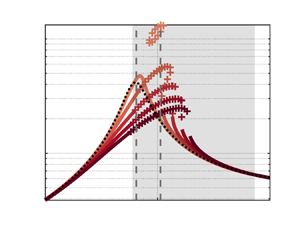
Figure 5. Weakly and fully nonlinear harmonic gain in the BFS flow (sketched in figure 2a). At each frequency and each Reynolds number, the optimal linear forcing structure  $\boldsymbol {\hat {f}}_o$ is applied. (a) Fixed frequency $\omega _o/(2{\rm \pi} ) = 0.075$, varying Reynolds number $Re=200$ and $700$ (larger $Re$ darker). Inset: log–log scale, $Re=200, 300, \ldots, 700$. (b) Fixed Reynolds number $Re=500$, varying forcing r.m.s. amplitude $F = \sqrt {2}^{-1} [1,2,4,10] \times 10^{-4}$ (larger amplitudes darker).
Next, we select  $Re=500$ and report in figure 5(b) harmonic gains as a function of the frequency, for increasing forcing amplitudes. At each frequency, the corresponding optimal forcing structure $\boldsymbol {\hat {f}}_o$ is applied. The comparison between DNS and WNNh is conclusive over the whole range of frequencies. The saturating character of nonlinearities is well captured. Such a good agreement may appear surprising in the low-frequency regime, for instance at $\omega _o / (2{\rm \pi} ) = 0.04$ where the second harmonics at frequency $2\omega _0$ could, in principle, be amplified approximately four times more than the fundamental. It happens, however, that the associated forcing structure $-C(\boldsymbol {\hat {u}}_o,\boldsymbol {\hat {u}}_o)$ is located much farther downstream than the optimal forcing at $2\omega _o$, with a weak overlap region which results in a poor projection. Therefore, the second-order contribution does not reach amplitudes of concern in this flow, as a consequence of its streamwise non-normality. For $\omega _o / (2{\rm \pi} ) = 0.075$ the fully nonlinear and predicted weakly nonlinear structures are compared in figure 6. The energy centroid of the fully nonlinear response shows a clear migration upstream when increasing the forcing amplitude, as already reported in Mantic-Lugo & Gallaire (Reference Mantic-Lugo and Gallaire2016b). It is associated with a shortening of the mean recirculation bubble under the action of the Reynolds stresses, in turn explaining the reduction of the gain. Although some distortion of the structures due to higher harmonics is observed when increasing the forcing amplitude, the fully nonlinear structure remains dominated by its $\omega _o$-component. The weakly nonlinear structure does not capture the upstream migration since it does not include the $O(\epsilon _o^{3/2})$ corrections of the $\omega _o$-component structure; thus, the latter is intrinsically restricted to $\boldsymbol {\hat {u}}_o$. However, the coefficient $\mu +\nu$ is constructed on forcing terms at $O(\epsilon _o^{3/2})$ and indeed embeds the nonlinear interactions responsible for the migration and the saturation, explaining why the predicted level of energy is correct even though the structure is not.

Figure 6. Snapshots of the weakly (WNNh) and fully (DNS) nonlinear cross-wise ( $y$) component of the velocity perturbation around the mean flow in the BFS flow. The frequency is fixed to $\omega _o/(2{\rm \pi} )=0.075$ and the Reynolds number to $Re=500$. Three increasing forcing amplitudes are considered: (a), (b) and (c) correspond respectively to $F=[10^{-5}, 10^{-4}\ {\rm and}\ 10^{-3}]/\sqrt {2}$. The WNNh structures are evaluated as $2\mathrm {Re}(\sqrt {\epsilon _o} A \textrm {e}^{\textrm {i}\omega _o t} \boldsymbol {\hat {u}}_o + \epsilon _o A^2 \textrm {e}^{2\textrm {i}\omega _o t} \boldsymbol {\hat {u}}_{2,2} )$, with $A$ the equilibrium solution of (2.12); the DNS structures are obtained by taking the $n\omega _o$ ( $n=1,2,3,\ldots$) Fourier components of a DNS simulation in the stationary regime, then by taking two times the real part of their sum weighted by $\textrm {e}^{\textrm {i} n \omega _o t}$. In this manner, the phases can also be compared between WNNh and DNS.
2.2. Application case: Orr mechanism in the plane Poiseuille flow
The weakly nonlinear evolution of the harmonic gain is now sought for the plane Poiseuille flow sketched in figure 2, a typical flow with component-wise non-normality (Trefethen et al. Reference Trefethen, Trefethen, Reddy and Driscoll1993; Schmid Reference Schmid2007). Periodicity is imposed in the streamwise and spanwise directions with wavenumbers  $k_x$ and $k_z$, respectively. The set of parameters $(Re,k_x,k_z) = (3000,1.2,0)$ is selected. According to the classical work of Orszag (Reference Orszag1971), the base flow at this $Re$ number is linearly stable since instability first occurs at $Re_{cr} \approx 5772$ and $k_{x,cr} \approx 1.02$. In both the linear and nonlinear computations, the spanwise invariance $k_z=0$ is systematically maintained. While the base flow $U(y)$ has only one velocity component and depends only on one coordinate, the perturbations are here two-dimensional (i.e. $\boldsymbol {u} = (u_x(x,y),u_y(x,y))$). The computations are performed in the streamwise-periodic box $(x,y) \in [0,2{\rm \pi} /1.2] \times [-1,1] \equiv \varOmega$. All the scalar products are taken upon integration inside this periodic box, in particular for the normalisation $\langle \boldsymbol {\hat {u}}_o,\boldsymbol {\hat {u}}_o\rangle = \langle \boldsymbol {\hat {f}}_o,\boldsymbol {\hat {f}}_o\rangle =1$, and latter for the evaluation of the weakly nonlinear coefficients.
The linear optimal gain (2.1) is computed in the frequency interval  $0 \leq \omega _o \leq 0.8$ (figure 7a), together with the associated optimal forcing and responses structures. Results are validated with the one-dimensional results of Schmid & Henningson (Reference Schmid and Henningson2001) based on a Fourier expansion of wavenumbers $k_x=1.2$ and $k_x=0$ in the streamwise direction. Eigenspectra are also reported in figure 7(b). The singular value decomposition (SVD) algorithm applied to the periodic box automatically selects the most amplified wavenumber among all spatial harmonics $n 1.2$ with $n=0,1,2,\ldots$. Below $\omega _o \approx 0.12$, the harmonic $0 \times 1.2 =0$ is dominant due to the concentration of weakly damped eigenvalues along the imaginary axis. The gain $G(\omega _o = 0) = 1216$ is equal to the inverse of the smallest damping rate among all these spatially invariant modes. The large value of the gain associated with those modes is understood considering that the small pressure gradient $(2/Re,0)^\textrm {T}=(2/3000,0)^\textrm {T}$ is sufficient to induce the Poiseuille base flow (equal to unity in the centreline). Above $\omega _o \approx 0.12$, the fundamental wavenumber $1 \times 1.2=1.2$ prevails. The corresponding harmonic gain presents a local and selective maximum for $\omega _o = 0.38$, certainly linked to the presence of the weakly damped eigenvalue $\sigma _1 = -0.0103+0.380\textrm {i}$. Nevertheless, $G(\omega _o =0.38) = 416$ is significantly larger than $1/0.0103 \approx 97$. This is a direct consequence of the non-normality of the plane Poiseuille flow. Unlike the BFS flow, the non-normality at play here is not due to the presence of a convectively unstable region but to the Orr mechanism, suggested for the first time in Orr (Reference Orr1907). Namely, an initial condition or forcing field constituted of spanwise vortices tilted towards the upstream direction (figure 8a), tilts downstream under the action of the mean shear (figure 8b), which leads to a significant gain in the kinetic energy of the perturbation. The coefficient $B$ is shown in figure 9(a), and the associated WNNh prolongation of the harmonic gain in figure 9(b). The coefficient $B$ is negative in the interval $0.378 \leq \omega _o \leq 0.486$, and $B$ and $D$ are such that three equilibrium amplitudes $\left | a_e \right |$ exist for some values of $F$ in the sub-interval $0.389 \leq \omega _o \leq 0.428$. Among them, none or only one is found to be stable. Consequently, as the forcing amplitude is increased, the harmonic gain curve leans toward the higher frequencies in figure 9(b); in the meantime, a frequency interval where no stable solution is predicted appears and grows larger.

Figure 7. (a) Linear harmonic (optimal) gain as function of the optimisation frequency. Present results are compared with those reproduced from Schmid & Henningson (Reference Schmid and Henningson2001), where perturbations are expressed as Fourier mode of streamwise wavenumber  $k_x$. (b) Eigenspectra.

Figure 8. (a) Streamwise component of the optimal forcing  $\mathrm {Re}(\,f_{o,x})$ for the plane Poiseuille flow (sketched in figure 2b) for $(Re,k_x,k_z) = (3000,1.2,0)$ and $\omega _o=0.3810$. (b) Streamwise component of the response $\mathrm {Re}(\hat {u}_{o,x})$. Both fields are normalised as $\|\boldsymbol {\hat {f}}_o\| = \|\boldsymbol {\hat {u}}_o\| = 1$. Only one wavelength $0 \leq k_x x \leq 2{\rm \pi}$ is shown.

Figure 9. (a) Coefficient  $B$ defined in (2.16) as a function of the optimisation frequency. The superimposed bold green line indicates that $B$ and $D$ are such that three equilibrium solutions to (2.14) exist. (b) Weakly nonlinear harmonic gain predicted by the WNNh model for increasing forcing amplitude $F$ in $[0.55, 1.45, 2.35, 3.25, 4.15] \times 10^{-4}$ (larger $F$ darker). Solid lines denote stable equilibrium solutions of (2.14) whereas bold plus markers (+) denote the unstable ones. The vertical dashed grey lines highlight $\omega _o=0.3810$ and $\omega _o=0.4025$, frequencies for which comparison with DNS data is shown in figure 10. The grey zone denotes a negative $B$.
$B$.
Note that, in the absence of a stable equilibrium, it is natural to consider completing (2.14) up to  $O(\sqrt {\epsilon _o}^{5})$. It is shown in Appendix C, however, that such an approach is problematic in the present case, because the non-oscillating forcing terms appearing at $O(\epsilon _o^2)$ excite the largely amplified static modes visible in figure 7 for $\omega _o =0$. The associated gains being of order $1/\epsilon _o$, the mean flow correction terms at $O(\epsilon _o^2)$ break the asymptotic hierarchy. This problem is not encountered at $O(\epsilon _o)$, because the forcing $-2C(\boldsymbol {\hat {u}}_o,\boldsymbol {\hat {u}}_o^*)$ in (2.10) projects poorly on the optimal one for $\omega _o=0$, and $\|\boldsymbol {u}_{2,0}\|$ remains of order unity.
For comparison with DNS data, two different forcing frequencies with a priori distinct behaviours are selected:  $\omega _o=0.3810$ and $\omega _o=0.4025$. These two frequencies are highlighted by the vertical dashed grey lines in figure 9. In both cases the coefficient $B$ is negative, and for the case $\omega _o=0.4025$ three equilibrium solutions exist for some values of $F$. The linear gains and weakly nonlinear coefficients are reported in table 2.
Table 2. The WNNh coefficients for the plane Poiseuille flow at  $(Re,k_x,k_z)=(3000,1.2,0)$, and when the optimal forcing structure ( $\gamma =1$) is applied.

The corresponding WNNh prolongation of the linear gain as a function of the forcing amplitude is shown in figure 10, together with DNS results. For comparison, the prediction of a ‘classical’ (modal) amplitude equation constructed around the weakly damped eigenvalue  $\sigma _1$ and its associated direct and adjoint modes is also added. Its derivation is briefly recalled in Appendix D.

Figure 10. Evolution of the harmonic gain  $G$ with respect to $F$ for (a) $\omega _o = 0.3810$ and (b) $\omega _o = 0.4025$ (frequencies highlighted by vertical dashed grey lines in figure 9). In both, the grey zone indicates that no harmonic gain could be properly defined, as the kinetic energy of the perturbation ceases to converge to a constant value. In particular, the inset shows the monitoring of $u_y(0,0)$ for the flow represented by the circle (the link is indicated by a thin line).
For  $\omega _o = 0.3810$ (figure 10a), the WNNh gain initially increases with $F$ due to the negativity of $B$. As visible in table 2, this is mostly due to the contribution of $\mathrm {Re}[\mu /(\epsilon _o \eta )]$ which is ten times larger than that of $\mathrm {Re}[\nu /(\epsilon _o \eta )]$. Thus, at this frequency, the principal factor for the initial increase of the WNNh gain is the Reynolds stress of the response $a \boldsymbol {\hat {u}}_o$. The latter creates a mean flow that amplifies the linear forcing $\boldsymbol {\hat {f}}_o$ more than the base flow does. This may be interpreted considering the displacement of the eigenvalue $\sigma _1$. Let $\boldsymbol {\hat {q}}_1$ (respectively $\boldsymbol {\hat {a}}_1$) denote the eigenmode (respectively adjoint mode) associated with the eigenvalue $\sigma _1$. The sensibility of the latter to the base flow deformation $\delta \boldsymbol {U}_b$ due to the Reynolds stress of $a \boldsymbol {\hat {u}}_o$ is written
 \begin{equation} \delta \sigma_1 ={-}\frac{\left \langle \boldsymbol{\hat{a}}_1, C[\boldsymbol{\hat{q}}_1,\delta \boldsymbol{U}_b] \right \rangle}{\left \langle \boldsymbol{\hat{a}}_1, \boldsymbol{\hat{q}}_1 \right \rangle}, \end{equation}
where  $\delta \boldsymbol {U}_b = |a|^2 \boldsymbol {u}_{2,0}$. For $\omega _o = 0.3810$, we obtain $\delta \sigma _1 = |a|^2 ( 1.2 + \textrm {i} \times 3.9)$. Since $\mathrm {Re}[\delta \sigma _1]>0$, the eigenvalue is moving towards the unstable part of the complex plane under the action of the Reynolds stress. This is in accordance with the fact that the plane Poiseuille flow is subcritical, and may explain the initial increase in the gain with $F$. Meanwhile, $\mathrm {Im}[\delta \sigma _1]>0$ and $\sigma _1$ is shifting toward higher frequencies. Thus $\omega _o$ ceases to be the least damped frequency, which could shed light on the fact that increasing $F$ further leads to a monotonic decay in the WNNh gain at $\omega _o$. Because of the flow non-normality, however, this explanation based solely on the location of $\sigma _1$ remains qualitative.
The overall agreement with the DNS results is excellent. Nevertheless, the WNNh model slightly underestimates the threshold in  $F$ above which a stable equilibrium does not exist anymore. It stands at $F/\epsilon _o = 0.087$ against $F/\epsilon _o =0.11$ for the DNS. This loss of a proper harmonic response may be symptomatic of the fact that $\sigma _1$ eventually crosses the neutral line and becomes unstable. Indeed, for $F/\epsilon _o =0.11$ (blue circle in the grey zone in figure 10a), the Fourier spectrum of the flow in its stationary regime presents two dominant neighbouring frequencies: the forcing one at $\omega = \omega _o$ and a second ‘natural’ one at $\omega \approx 0.404$. As these two frequencies are very close, a beating behaviour is visible in the inset of figure 10(a) at a frequency consistent with $\Delta \omega =0.404-0.381=0.023$.
The classical modal amplitude equation leads to a prediction that is only qualitative. Even for  $F=0$ the linear harmonic gain $|\langle \boldsymbol {\hat {f}}_o , \boldsymbol {\hat {a}}_1 \rangle /(\langle \boldsymbol {\hat {q}}_1 , \boldsymbol {\hat {a}}_1 \rangle \sigma _{1,r})|$ (see Appendix D for its derivation) is overestimated, as it is deduced from the modal quantities linked to $\sigma _1$ only. As mentioned earlier, in non-normal flows a high number of eigenmode is generally necessary to describe its harmonic response, even in the presence of a weakly damped eigenvalue. Thus, relying on a single mode constitutes a poor description of the response to forcing.
We now consider  $\omega _o=0.4025$, and the associated results in figure 10(b). The WNNh model yields multiple equilibrium solutions in the range $0 < F/\epsilon _o < 0.0264$. Only the one represented by a thick continuous line is stable, and corresponds to a monotonic growth of the gain with $F$. The DNS results validate the existence of this solution. The two other solutions, depicted by the dash-dotted and dashed lines, are unstable in one eigendirection and two eigendirections, respectively. Above $F/\epsilon _o = 0.0264$ the WNNh models predicts the loss of the stable equilibrium solution, which is accurately confirmed by the DNS whose threshold is located around $F/\epsilon _o = 0.0286$. Slightly above, the signal of $u_y(0,0)$ in the inset suggests again the presence of a ‘natural’ frequency due to the subcritical destabilisation of $\sigma _1$. Indeed, $u_y(0,0)$ alternates between an algebraic growth typical of a true resonance (both natural and forcing frequencies collapse), and a beating-like behaviour whose period is very long (the natural frequency drifts slightly from the forcing one).
Across this threshold, the evolution of the average kinetic energy of the response appears discontinuous. This loss of a stable equilibrium is to be distinguished with its destabilisation encountered for  $\omega =0.3810$. Overall, the difference of behaviours between figures 10(a) and 10(b) may be explained by the difference of proximity between $\omega _o$ and $\mathrm {Im}[\sigma _1]$ of the mean flow. As the forcing is progressively increased above $F/\epsilon _o = 0.0286$, the flow response quickly becomes chaotic, and then turbulent.
It should be mentioned that, in some situations, the amplitude equation (2.14) may be in default. First, as just mentioned, when the optimal linear harmonic gain at frequency  $2\omega _o$ is $\sim 1/\sqrt {\epsilon _o}$ or larger and projects well onto the optimal forcing, the asymptotic hierarchy is threatened as $\boldsymbol {\hat {u}}_{2,2}$ may be substantial enough to reach order $\sqrt {\epsilon _o}$ or above. It is thus important to assess that the norm of $\boldsymbol {\hat {u}}_{2,2}$ remains of order one. A second delicate situation arises, for the same reason, when a sub-optimal gain at the frequency $\omega _o$ is $\sim 1/\epsilon _o$. In both cases, the model could be extended by including in the kernel of $\varPhi$ the optimal response at frequency $2\omega _o$, or the sub-optimal response at frequency $\omega _o$, respectively.
Eventually, it should be noted that there are several manners to perturb  $R(\textrm {i}\omega _o)^{-1}$ such as to include $\boldsymbol {\hat {u}}_o$ in the kernel. Among them, the one with the smallest amplitude, i.e. $\epsilon _o$, has been chosen in (2.3). We demonstrate in Appendix E that this is the only choice that leads to a consistent amplitude equation. Choosing a higher perturbation amplitude is possible, but implies filling the kernel with another structure than $\boldsymbol {\hat {u}}_o$.
3. Transient growth
Next, we derive an amplitude equation for the weakly nonlinear transient growth in an unforced ( $\boldsymbol {f}=\boldsymbol {0}$) system, without restriction on its linear stability.
The solution to the linearised equation (1.2) is  $\boldsymbol {u}(t) = \textrm {e}^{L t}\boldsymbol {u}(0)$, where $\textrm {e}^{L t}$ is the operator exponential of $L t$. In an unforced context, the propagator $\textrm {e}^{ L t}$ maps an initial structure at time $t=0$ onto its evolution at $t \geq 0$. The largest linear amplification at $t_o>0$ (subscript $o$ for ‘optimal’) is
 \begin{equation} G(t_o) = \max_{\boldsymbol{u}(0)} \frac{\left \| \boldsymbol{u}(t_o) \right \| }{\left \| \boldsymbol{u}(0)\right \| } = \left \| {\rm e}^{L t_o} \right \| \doteq \frac{1}{\epsilon_o}. \end{equation}
The singular-value decomposition of the propagator  $\textrm {e}^{L t_o}$ provides the transient gain $G(t_o)$ as the largest singular value of $\textrm {e}^{L t_o}$, as well as the left and right singular pair $\boldsymbol {v}_o$ and $\boldsymbol {u}_o$, respectively,
 \begin{equation} {\rm e}^{- L t_o} \boldsymbol{v}_o = \epsilon_o \boldsymbol{u}_o, \quad \left[ \left( {\rm e}^{ L t_o} \right)^{\dagger} \right]^{{-}1} \boldsymbol{u}_o = \epsilon_o \boldsymbol{v}_o, \end{equation}
where  $\|\boldsymbol {v}_o\| = \| \boldsymbol {u}_o\| = 1$. The field $\boldsymbol {u}_o$ is the optimal initial structure for the propagation time $t=t_o$, and $\boldsymbol {v}_o$ is its normalised evolution at $t_o$. The corresponding amplification is $1/\epsilon _o$, as defined in (3.1). Smaller singular values are sub-optimal gains, associated with orthogonal sub-optimal initial conditions. Their orthogonality is ensured by the fact that singular vectors of the operator $\textrm {e}^{L t_o}$ also are the eigenvectors of the symmetric operator $(\textrm {e}^{L t_o})^{\dagger} \textrm {e}^{L t_o}$, the singular values of the former being the square root of the eigenvalues of the latter. Of all the $t_o$, the time leading to the largest optimal gain will be highlighted with the subscript $m$ (for ‘maximum’) such that $\max _{t_o>0} G(t_o) = G(t_{o,m})$.
By construction, the linear gain is independent of the amplitude of the initial condition  $\boldsymbol {u}(0)$. As this amplitude increases, however, nonlinearities may come into play and the nonlinear gain may depart from the linear gain $G$. Similar to the previous section on harmonic gain, we propose a method for capturing the effect of weak nonlinearities on the transient gain.
Due to the assumed non-normality of  $L$, the inverse gain is small, $\epsilon _o \ll 1$. While the previous section focused on the inverse resolvent, it is now the inverse propagator $\textrm {e}^{-Lt_o}$ that appears close to singular. The first equality of (3.2) can be rewritten as $(\textrm {e}^{- L t_o} - \epsilon _o \boldsymbol {u}_o \langle \boldsymbol {v}_o,*\rangle ) \boldsymbol {v}_o = \boldsymbol {0}$, which shows that the operator $(\textrm {e}^{- L t_o} - \epsilon _o \boldsymbol {u}_o \langle \boldsymbol {v}_o,*\rangle )$ is singular since $\boldsymbol {v}_o \neq \boldsymbol {0}$ belongs to its kernel. Mirroring our previous reasoning for the WNNh model, we now wish to construct a perturbed inverse propagator whose kernel is the linear trajectory
 \begin{equation} \boldsymbol{l}(t) \doteq \epsilon_o {\rm e}^{L t} \boldsymbol{u}_o, \end{equation}
seeded by the optimal initial condition  $\boldsymbol {u}_o$ and of unit norm in $t=t_o$ since $\boldsymbol {l}(t_o) = \boldsymbol {v}_o$. One conceptual difficulty lies in the fact that the linear response is not a fixed vector field, but a time-dependent trajectory; therefore, the perturbed inverse propagator too should depend on time. We propose to perturb the inverse propagator for all $t \geq 0$ as
 \begin{equation} \varPhi(t) = {\rm e}^{{-}L t} - \epsilon_o P(t), \quad \text{where} \ P(t) \doteq H(t) \frac{\boldsymbol{u}_o \langle \boldsymbol{l}(t),*\rangle}{\left \| \boldsymbol{l}(t) \right \|^2}, \end{equation}
and where the Heaviside distribution  $H(t)$ satisfies $H(0)=0$ and $H(t>0)=1$. As the time $t \rightarrow t_o$, the perturbation operator $P \rightarrow \boldsymbol {u}_o \langle \boldsymbol {v}_o,*\rangle$ such that $\|P\| \rightarrow 1$ and the expansion (3.4) is certainly justified. The non-trivial kernel of $\varPhi (t)$ is $\boldsymbol {l}(t)$ for all $t>0$; the kernel reduces to $\boldsymbol {0}$ at $t=0$ since $\varPhi (0)= I$. We show in addition that, for $t>0$, the non-trivial kernel of the adjoint operator $\varPhi (t)^{\dagger}$ is
 \begin{equation} \boldsymbol{b}(t) \doteq \left( {\rm e}^{L t} \right)^{\dagger}\boldsymbol{l}(t). \end{equation}
Indeed, using that  $P^{\dagger} = \boldsymbol {l}(t)\langle \boldsymbol {u}_o,* \rangle / \langle \boldsymbol {l}(t) , \boldsymbol {l}(t) \rangle$ for $t>0$, we have
 \begin{align} \varPhi(t)^{\dagger} \boldsymbol{b}(t) &= \left({\rm e}^{- L t}\right)^{\dagger} \boldsymbol{b}(t) - \epsilon_o \boldsymbol{l}(t) \frac{\left \langle \boldsymbol{u}_o , \boldsymbol{b}(t) \right \rangle}{\left \langle \boldsymbol{l}(t) , \boldsymbol{l}(t) \right \rangle}\nonumber\\ & = \left({\rm e}^{- L t}\right)^{\dagger} \boldsymbol{b}(t) - \epsilon_o \boldsymbol{l}(t) \frac{\left \langle {\rm e}^{L t}\boldsymbol{u}_o , \boldsymbol{l}(t) \right \rangle}{\left \langle \boldsymbol{l}(t) , \boldsymbol{l}(t) \right \rangle}\nonumber\\ & = \left({\rm e}^{- L t}\right)^{\dagger} \boldsymbol{b}(t) - \boldsymbol{l}(t) \nonumber\\ & = \left[\left({\rm e}^{ L t}\right)^{\dagger} \right]^{{-}1} \boldsymbol{b}(t) - \boldsymbol{l}(t) \nonumber\\ & = \boldsymbol{0}. \end{align}
 As an illustration of the singularisation of  $\textrm {e}^{-Lt_o}$, parts of the spectra of $\textrm {e}^{-Lt_o}$ and $\varPhi (t_o)$ are shown in figure 11 for the plane Poiseuille flow sketched in figure 2. The red dot at the origin is the null singular eigenvalue of $\varPhi (t_o)$ associated with $\boldsymbol {l}(t_o)$. Since $\|P(t_o)\|=1$, this singular eigenvalue lies on the $\epsilon _o$-pseudospectrum of $\textrm {e}^{-Lt_o}$, meaning that a perturbation of amplitude $\epsilon _o$ is sufficient to make the inverse propagator singular.

Figure 11. Restricted spectra (fifteen least stable eigenvalues) of the natural and perturbed inverse propagators of the plane Poiseuille flow (sketched in figure 2b) for  $t=t_o=10$ and $(Re,k_x,k_z)=(3000,0.5,2)$ (purely one-dimensional computations using the code of Schmid & Henningson (Reference Schmid and Henningson2001) based on a Fourier expansion of wavenumbers $k_x$ and $k_z$ in $x$ and $z$, respectively). Blue circles: eigenvalues of $\textrm {e}^{-Lt_o}$. Red dots: eigenvalues of $\varPhi (t_o)$. By construction, one eigenvalue of $\varPhi (t)$ lies at the origin. Thin red lines: full locus of the eigenvalues of $\varPhi (t)$ for $t \leq t_o$. Green line: $\epsilon _o$-pseudospectrum of $\textrm {e}^{-Lt_o}$, such that $\| (\textrm {e}^{-Lt_o} -z I)^{-1} \| = 1/\epsilon _o$.
Recalling that  $L$ is assumed strongly non-normal, we choose $\epsilon _o \ll 1$ as expansion parameter, introduce the slow time scale $T = \epsilon _o t$ and propose the multiple-scale expansion
 \begin{equation} \boldsymbol{U}(t,T) = \boldsymbol{U}_e + \epsilon_o\boldsymbol{u}_1(t,T) + \epsilon_o^2 \boldsymbol{u}_2(t,T) + O(\epsilon_o^3). \end{equation}
The square root scaling of the previous section is not made here, as resonance at second order cannot be excluded a priori. The flow is initialised with  $\boldsymbol {U}(0) = \alpha \epsilon _o^2 \boldsymbol {u}_o$, where $\alpha = O(1)$ is a prefactor. After injecting this expansion in the unforced Navier–Stokes equations, we obtain
 \begin{equation} \epsilon_o (\partial_t - L)\boldsymbol{u}_1 + \epsilon_o^2 \left[ (\partial_t - L)\boldsymbol{u}_2 + C(\boldsymbol{u}_1,\boldsymbol{u}_1) + \partial_T \boldsymbol{u}_1 \right] + O(\epsilon_o^3) = \boldsymbol{0}, \end{equation}
subject to  $\boldsymbol {u}_2(0) = \alpha \boldsymbol {u}_o$, and $\boldsymbol {u}_i(0) = \boldsymbol {0}$ for $i\neq 2$. In its primary quality of inverse propagator, the following property holds for $\textrm {e}^{-L t}$: $\partial _t (\textrm {e}^{-Lt}) = -\textrm {e}^{-Lt}L$, where the commutation of $\textrm {e}^{-Lt}$ and $L$ has not been used. Thanks to this relation, we write $(\partial _t - L)\boldsymbol {u}_i = \textrm {e}^{L t} \partial _t (\textrm {e}^{-L t}\boldsymbol {u}_i )$. As a result, $L$ disappears from the asymptotic expansion but $\textrm {e}^{-L t}$ appears. The latter is perturbed according to (3.4), leading to $\textrm {e}^{L t} \partial _t (\textrm {e}^{-L t}\boldsymbol {u}_i ) = \textrm {e}^{L t} \partial _t (\varPhi (t) \boldsymbol {u}_i ) + \epsilon _o \textrm {e}^{L t} \partial _t (P(t) \boldsymbol {u}_i)$ for $i=1,2,\ldots$. The asymptotic expansion (3.8) becomes
 \begin{align} \epsilon_o {\rm e}^{L t}\partial_t (\varPhi \boldsymbol{u}_1) + \epsilon_o^2 \left[ {\rm e}^{L t}\partial_t (\varPhi \boldsymbol{u}_2) + C(\boldsymbol{u}_1,\boldsymbol{u}_1) + \partial_T \boldsymbol{u}_1 + {\rm e}^{L t}\partial_t ( P(t) \boldsymbol{u}_1) \right] + O(\epsilon_o^3) = \boldsymbol{0}. \end{align}
Note that the transformation performed from (3.8) to (3.9) is not restricted to time-independent base flows, as the property  $\partial _t(\varPsi (t)^{-1})= -\varPsi (t)^{-1}L(t)$ holds for a time-varying operator $L(t)$ and the associated propagator $\varPsi (t)$. This can be shown easily by taking the time derivative of $\varPsi (t)^{-1}\boldsymbol {u}(t) = \boldsymbol {u}(0)$. Terms of (3.9) are then collected at each order in $\epsilon _o$, leading to a succession of linear problems, detailed hereafter.
At order  $\epsilon _o$, we collect $\partial _t (\varPhi \boldsymbol {u}_1) = \boldsymbol {0}$, subject to $\boldsymbol {u}_1(0) = \boldsymbol {0}$. We obtain $\varPhi \boldsymbol {u}_1 = \varPhi (0)\boldsymbol {u}_1(0) = \boldsymbol {0}$, therefore $\boldsymbol {u}_1(t,T)$ is proportional to the kernel of $\varPhi (t)$ for all $t \geq 0$. We choose the non-trivial solution
 \begin{equation} \boldsymbol{u}_1(t,T) = A(T)H(t)\boldsymbol{l}(t), \end{equation}
where the initial condition  $\boldsymbol {u}_1(0)=\boldsymbol {0}$ is enforced by $H(t)$, while the slowly varying scalar amplitude $A(T)$ is continuous in $T$ and modulates the linear trajectory. This choice is motivated by the observation that, since $A$ must be constant in time in the linear regime, we expect it to be weakly time dependent in the weakly nonlinear regime. We stress that $A(T)$ does not depend explicitly on $t$, such that $\partial _t A =0$. Note that the choice $\boldsymbol {u}_1(t) = A(t)H(t)\boldsymbol {l}(t)$ would also have been possible, and the assumption of the amplitude depending on a slow time scale is made solely to simplify the ensuing calculations.
At order  $\epsilon _o^2$, we collect
 \begin{equation} \partial_t (\varPhi \boldsymbol{u}_2) + A^2 H {\rm e}^{{-}L t}C(\boldsymbol{l},\boldsymbol{l}) + H \frac{\mathrm{d} A}{\mathrm{d} T} {\rm e}^{{-}L t} \boldsymbol{l} + A {d}_t (H P \boldsymbol{l}) = \boldsymbol{0}, \end{equation}
subject to  $\boldsymbol {u}_2(0) = \alpha \boldsymbol {u}_o$. We used the property $H(t)^2=H(t)$, which will henceforth be understood. The particular solution of (3.11) yields
 \begin{equation} \boldsymbol{u}_2(t,T)= \boldsymbol{u}_2^{(a)}(t) + A(T)^2\boldsymbol{u}_2^{(b)}(t) + \frac{\mathrm{d} A(T)}{\mathrm{d} T}\boldsymbol{u}_2^{(c)}(t) + A(T)\boldsymbol{u}_2^{(d)}(t), \end{equation}
where
 \begin{equation} \left. \begin{aligned} & {d}_t\left(\varPhi \boldsymbol{u}_2^{(a)}\right) =\boldsymbol{0}, \quad {d}_t\left(\varPhi \boldsymbol{u}_2^{(b)}\right) ={-} H\,{\rm e}^{{-}Lt}C(\boldsymbol{l},\boldsymbol{l}),\\ & {d}_t \left(\varPhi \boldsymbol{u}_2^{(c)}\right) ={-} H {\rm e}^{{-}Lt}\boldsymbol{l} , \quad \text{and} \quad {d}_t\left(\varPhi \boldsymbol{u}_2^{(d)}\right) ={-} {d}_t\left(H P \boldsymbol{l} \right), \end{aligned} \right\} \end{equation}
subject to the initial conditions  $\boldsymbol {u}_2^{(a)}(0) = \alpha \boldsymbol {u}_o$ and $\boldsymbol {u}_2^{(b)}(0) = \boldsymbol {u}_2^{(c)}(0) = \boldsymbol {u}_2^{(d)}(0) = \boldsymbol {0}$. Time integration can now be performed without ambiguity as all the partial derivatives ( $\partial _t \cdots$) have been replaced by total derivatives ( ${d}_t\ldots$). After time integration between $t=0$ and $t>0$, we obtain a series of problems for $\boldsymbol {u}_2^{(a)}$, $\boldsymbol {u}_2^{(b)}$, $\boldsymbol {u}_2^{(c)}$ and $\boldsymbol {u}_2^{(d)}$
 \begin{equation} \varPhi(t) \boldsymbol{u}_2^{(a)}(t)=\varPhi(0) \boldsymbol{u}_2^{(a)}(0) = \alpha \boldsymbol{u}_o, \end{equation}
since  $\varPhi (0)=I$;
 \begin{equation} \varPhi(t) \boldsymbol{u}_2^{(b)}(t)={-} \int_{0}^{t} H(s){\rm e}^{{-}Ls}C[\boldsymbol{l}(s),\boldsymbol{l}(s)]\,\mathrm{d}s = {\rm e}^{{-}Lt}\tilde{\boldsymbol{u}}_2(t), \end{equation}
where
 \begin{equation} \frac{\mathrm{d} \tilde{\boldsymbol{u}}_2 }{\mathrm{d} t} = L \tilde{\boldsymbol{u}}_2 - C(\boldsymbol{l},\boldsymbol{l}), \quad \tilde{\boldsymbol{u}}_2(0) = \boldsymbol{0}, \end{equation}
and where we have used that the general solution of  ${d}_t \boldsymbol {x} =L\boldsymbol {x} + \boldsymbol {F}$ is $\boldsymbol {x}(t) = \textrm {e}^{Lt}[\boldsymbol {x}(0) + \int _{0}^{t}\textrm {e}^{-Ls} \boldsymbol {F}(s)\mathrm {d}s]$;
 \begin{align} \varPhi(t) \boldsymbol{u}_2^{(c)}(t) &={-} \int_{0}^{t} H(s) {\rm e}^{{-}Ls}\boldsymbol{l}(s) \,\mathrm{d}s \nonumber\\ & ={-} \int_{0}^{t} H(s) \epsilon_o \boldsymbol{u}_o\,\mathrm{d}s={-} \epsilon_o \boldsymbol{u}_o t, \end{align}
since  $\textrm {e}^{-L t} \boldsymbol {l}(t) = \epsilon _o \boldsymbol {u}_o$ holds by construction; and
 \begin{equation} \varPhi(t) \boldsymbol{u}_2^{(d)}(t) ={-}\left[H(t) P(t) \boldsymbol{l}(t) - H(0) P(0) \boldsymbol{l}(0)\right] ={-} \boldsymbol{u}_o, \end{equation}
since, by construction,  $H(t) P(t) \boldsymbol {l}(t) = H(t) \boldsymbol {u}_o$. Note that the presence of the Heaviside distribution inside the integral is unimportant. Eventually,
 \begin{equation} \varPhi \boldsymbol{u}_2 = \alpha \boldsymbol{u}_o + A^2 {\rm e}^{{-}L t} \tilde{\boldsymbol{u}}_2 - \epsilon_o t \frac{\mathrm{d} A }{\mathrm{d} T} \boldsymbol{u}_o - A \boldsymbol{u}_o, \quad t>0. \end{equation}
 Invoking again the Fredholm alternative, (3.19) admits a non-diverging particular solution if and only if its right-hand side is orthogonal to  $\boldsymbol {b}(t)$ for all $t>0$. This leads to
 \begin{equation} \left \langle \boldsymbol{u}_o , \boldsymbol{b}(t) \right \rangle \left(\alpha - A \right) + A^2 \left \langle {\rm e}^{{-}Lt}\tilde{\boldsymbol{u}}_2(t),\boldsymbol{b}(t) \right \rangle - \epsilon_o t \frac{\mathrm{d} A}{\mathrm{d} T}\left \langle \boldsymbol{u}_o , \boldsymbol{b}(t) \right \rangle = 0, \quad t>0. \end{equation}
Dividing (3.20) by  $\langle \boldsymbol {u}_o , \boldsymbol {b}(t) \rangle$ leads to
 \begin{equation} \left(\alpha - A \right) + \epsilon_o A^2 \mu_2(t) - \epsilon_o t \frac{\mathrm{d} A}{\mathrm{d} T} = 0, \quad t>0, \end{equation}
where
 \begin{equation} \mu_2(t) = \epsilon_o^{{-}1}\frac{\left \langle {\rm e}^{{-}Lt} \tilde{\boldsymbol{u}}_2(t) , \boldsymbol{b}(t) \right \rangle}{\left \langle \boldsymbol{u}_o, \boldsymbol{b}(t) \right \rangle} = \frac{\left \langle \tilde{\boldsymbol{u}}_2(t) , \boldsymbol{l}(t) \right \rangle}{\left \langle \boldsymbol{l}(t), \boldsymbol{l}(t) \right \rangle}. \end{equation}
Equation (3.21) is re-expressed as  $E(t,T) = 0$ for $t>0$, where $E(t,T) = (\alpha - A ) + \epsilon _o A^2 \mu _2(t) - \epsilon _o t \mathrm {d}_T A$. Since $\int _{t\rightarrow 0}^{t}\partial _s E(s,T)\,\mathrm {d}s = E(t,T)-E(t\rightarrow 0,T)$, solving $E(t,T) = 0$ is equivalent to solving $\partial _t E(t,T)=0$ for $t>0$ subject to $E(t\rightarrow 0,T) = 0$. Thereby, the partial derivative of (3.21) with respect to the short time scale $t$ is taken, leading to
 \begin{equation} \epsilon_o A^2 \frac{\mathrm{d} \mu_2(t)}{\mathrm{d} t} - \epsilon_o \frac{\mathrm{d} A}{\mathrm{d} T} = 0, \quad 0 < t, \end{equation}
where we have used that  $\partial _t A= 0$ by construction since $A=A(T)$ does not explicitly depend on $t$. Furthermore, the relation (3.23) is subject to $E(t\rightarrow 0,T) = \lim _{t\rightarrow 0} ( \alpha - A ) =0$ where we have used that $\tilde {\boldsymbol {u}}_2(t \rightarrow 0) = \tilde {\boldsymbol {u}}_2(0) = 0$. To be meaningful, (3.23) and its initial condition must be re-written solely in terms of $t$, which is done by evaluating $T$ along $T=\epsilon _o t$. The total derivative of $A$, denoted $d_t A$, is now needed, as it takes into account the implicit dependence of $A$ on $t$. By definition, $d_t A = \partial _t A + \epsilon _o \partial _T A = \epsilon _o d_T A$, such that the final amplitude equation reads
 \begin{equation} \frac{\mathrm{d} A}{\mathrm{d} t} = \epsilon_o A^2\frac{\mathrm{d} \mu_2(t)}{\mathrm{d} t} , \quad \text{with} \ A(0) = \alpha, \end{equation}
as  $\lim _{t\rightarrow 0} ( \alpha - A(\epsilon _o t) ) = 0$ implies $A(t\rightarrow 0) = \alpha$, and the amplitude $A$ is extended by continuity in $t=0$ so as to eventually impose $A(0) = \alpha$. Note that the evaluation in $T=\epsilon _o t$ and the passage to the total derivative would lead to indeterminacy in its solution if performed directly in (3.21), since that equation is not subject to any initial condition. Indeed, at linear level for instance, it would yield ${d}_t A = (\alpha -A)/t$, which admits the family of solutions $A(t) = \alpha + C t$, with $C$ an undetermined constant.
We stress that the inverse propagator is not needed to solve the amplitude equation (3.24). Just like the original problem considered in this section, (3.24) is unforced and has a non-zero initial condition. In the linear regime,  $A=\alpha$ for all times, and the linear gain is $\| \epsilon _o \alpha \boldsymbol {l}(t) \|/ \| \alpha \epsilon _o^2 \| = \| \boldsymbol {l}(t) \|/ \epsilon _o$. At $t=t_o$, in particular, we recover that it is equal to $1/\epsilon _o$ since $\| \boldsymbol {l}(t_o) \|= \| \boldsymbol {v}_o \|=1$.
In the following, we call equation (3.24) the Weakly Nonlinear Non-normal transient (WNNt) model. It can be corrected with higher-order terms, which requires solving the linear singular system (3.19), as detailed in Appendix F. We show in particular that singular higher-order solutions are orthogonal to the first-order solution  $\boldsymbol {l}(t)$, and that the action of $\varPhi$ need not be computed explicitly but can in practice be replaced by the action of $\textrm {e}^{-Lt}$.
3.1. Application case: the flow past a BFS
The WNNt model is applied to the BFS flow for  $Re=500$ and $t_o = t_{o,m} = 58$. See Appendix B for details about the numerical method. For these parameters, the linear optimal structures (figure 12) and gain are validated with the results presented in Blackburn et al. (Reference Blackburn, Barkley and Sherwin2008). The quadratic term in (3.24), although asymptotically correct, happens to be insufficient to capture the nonlinear saturation of the transient gain for this particular flow, in particular because of the weak value of the coefficient $\mu _2(t)$. Indeed, $\boldsymbol {l}(t_o) = \boldsymbol {v}_o$ appears to be dominated by a specific spatial wavenumber (see figure 12b), thus the field $\tilde {\boldsymbol {u}}_2$, being generated by the nonlinear interaction of $\boldsymbol {l}(t)$ with itself, is dominated by spatial harmonics and its projection on $\boldsymbol {l}(t)$ is close to zero. For this flow the WNNt model therefore needs to be extended to order $\epsilon _o^3$ (see Appendix F), yielding
 \begin{equation} \frac{\mathrm{d} A}{\mathrm{d} t} = \epsilon_o A^2 \frac{\mathrm{d} \mu_2 }{\mathrm{d} t} + \epsilon_o^2 A^3 \frac{\mathrm{d} \mu_3 }{\mathrm{d} t}, \quad A(0)=\alpha, \end{equation}
where
 \begin{equation} \mu_3(t) \doteq \frac{\left \langle \tilde{\boldsymbol{u}}_3(t) , \boldsymbol{l}(t) \right \rangle}{\left \langle \boldsymbol{l}(t), \boldsymbol{l}(t) \right \rangle}, \end{equation}
and
 \begin{equation} \frac{\mathrm{d} \tilde{\boldsymbol{u}}_3}{\mathrm{d} t} = L\tilde{\boldsymbol{u}}_3 - 2\left[C(\boldsymbol{l},\tilde{\boldsymbol{u}}_2) - \mu_2 C(\boldsymbol{l},\boldsymbol{l}) + \dot{\mu}_2(\tilde{\boldsymbol{u}}_2- \mu_2\boldsymbol{l}) \right], \quad \tilde{\boldsymbol{u}}_3(0) = \boldsymbol{0}. \end{equation}
Equation (3.25) is similar to (3.24), although corrected by a cubic term. We formulate the amplitude equation (3.25) in terms of the rescaled quantities  $a = \epsilon _o A$ and the amplitude of the initial condition $U_0 =\|\boldsymbol {U}(0)\|=\alpha \epsilon _o^2$
 \begin{equation} \frac{\mathrm{d} a}{\mathrm{d} t} = a^2\frac{\mathrm{d}\mu_2}{\mathrm{d} t} + a^3\frac{\mathrm{d}\mu_3}{\mathrm{d} t},\quad a(0)=\frac{U_0}{\epsilon_o}. \end{equation}
In this manner, the weakly nonlinear transient gain becomes  $G(t_o) = a(t_o)/U_0$. Note that in (3.28) the amplitude $a(t)$ does not depend on $U_0$ nor on $\epsilon _o$ independently, but on their ratio $U_0/\epsilon _o$. Thus, as expected, increasingly nonlinear regimes are found when the amplitude of the initial condition increases with respect to the linear gain.

Figure 12. (a) Streamwise ( $x$) component of the optimal initial condition $\boldsymbol {u}_o$ for the BFS (sketched in figure 2a) at $Re=500$ and at $t_o = t_{o,m} = 58$. (b) Streamwise component of the evolution $\boldsymbol {v}_o$ at $t=t_o$. Both structures are normalised as $\|\boldsymbol {u}_o\| = \|\boldsymbol {v}_o\| = 1$.
Predictions from (3.28) are shown in figure 13 together with the linear and fully nonlinear DNS gain evaluated as  $G_{tot}(t) = \| \boldsymbol {U}(t) - \boldsymbol {U}_e \|/U_0$. In figure 13(a), the WNNt model extended to $O(\epsilon _o^3)$ appears to capture the weakly evolution of the transient gain with satisfactory precision. When the amplitude of the initial condition is too large, the higher-order fields $\tilde {\boldsymbol {u}}_2$, $\tilde {\boldsymbol {u}}_3$, $\ldots$ are expected to have a significant amplitude, and thus the WNNt prediction deteriorates since it is based on an asymptotic hierarchy. In figure 13(b), the gain history of $G_{tot}(t)$ for all times $0 \leq t \leq t_o$ is successfully compared with $a(t)\|\boldsymbol {l}(t)\|/U_0$. The coefficient $\mu _3(t)$ is much larger than $\mu _2(t)$ (inset), and is largely dominated by the part of $\tilde {\boldsymbol {u}}_3$ generated by the forcing term $C(\boldsymbol {l},\tilde {\boldsymbol {u}}_2)$. Since $\mu _3(t)$ is monotonically decreasing toward $\mu _3(t_o) = -7.77$, larger times are subject to a stronger saturation. This leads to a decrease of the time for which the specific initial condition $\boldsymbol {u}_o$ leads to a maximum transient gain, consistently with the DNS results.

Figure 13. Transient gain in the flow past a BFS (sketched in figure 2a) for  $Re = 500$. (a) Gain squared $G(t_o)^2$ for $t_o=t_{o,m}=58$ as a function of the amplitude of the initial condition. (b) History of the gain squared for $0\leq t \leq t_{o,m}$ and for three amplitudes of initial condition, $U_0/\epsilon _o = [0.025,0.08,0.25]$ (vertical dashed lines in (a)); larger amplitudes darker. Inset: weakly nonlinear coefficients $\mu _2(t)$ (continuous line) and $\mu _3(t)$ (dashed-dotted line) as a function of time.
3.2. Application case: lift-up in the plane Poiseuille flow
The WNNt is now applied to the plane Poiseuille flow. The set of parameters  $(Re,k_x,k_z,t_o) = (3000,0,2,t_{o,m}=230)$ is selected. In both the linear and nonlinear computations, the wavenumber $k_x=0$ is maintained such that the fields are constant in $x$, and only the dependence in $y$ and $z$ is computed. Contrarily to the application case § 2.2, perturbations can now be fully three-dimensional (i.e. $\boldsymbol {u}=(u_x(y,z),u_y(y,z),u_z(y,z))$. The computations are performed in the spanwise-periodic box $(y,z) \in [-1,1] \times [-{\rm \pi} /2,{\rm \pi} /2] \equiv \varOmega$. All the scalar products are taken upon integration inside this periodic box, in particular for the normalisation $\langle \boldsymbol {u}_o,\boldsymbol {u}_o\rangle = \langle \boldsymbol {v}_o,\boldsymbol {v}_o\rangle =1$, and for the evaluation of the weakly nonlinear coefficients. The linear optimal gain is validated with the result of Schmid & Henningson (Reference Schmid and Henningson2001); the associated optimal initial condition and its evolution at $t=t_o$ are shown in figures 14(a) and 14(b), respectively. The optimal initial condition consists of vortices aligned in the streamwise direction; as these streamwise vortices are superimposed on the parabolic base flow, they bring low-velocity fluid from the wall towards the channel centre and high-velocity fluid from the centre of the channel towards the walls, thus generating alternated streamwise streaks. Due to the spanwise periodicity of the optimal initial condition $\boldsymbol {u}_o$, all the solutions at even orders $\epsilon _o^{2n}$ $(n=1,2,3,\ldots )$ only yield even spatial harmonics in $k_z$ and are orthogonal to $\boldsymbol {l}(t)$, such that the coefficient $\mu _2(t)$ defined in (3.22) is null at all times. Therefore, (3.28) reduces to
 \begin{equation} \frac{\mathrm{d} a}{\mathrm{d} t} = a^3\frac{\mathrm{d} \mu_3 }{\mathrm{d} t},\quad a(0)=\frac{U_0}{\epsilon_o}, \end{equation}
and  $\tilde {\boldsymbol {u}}_3$ solves the simplified equation
 \begin{equation} \frac{\mathrm{d} \tilde{\boldsymbol{u}}_3 }{\mathrm{d} t} = L\tilde{\boldsymbol{u}}_3 - 2C(\tilde{\boldsymbol{u}}_2,\boldsymbol{l}), \quad \tilde{\boldsymbol{u}}_3(0) = \boldsymbol{0}. \end{equation}
The analytical solution of (3.29) is written
 \begin{equation} a(t)= \frac{U_0}{\epsilon_o}\left[ 1-\left( \frac{U_0}{\epsilon_o} \right)^2 2\mu_3(t) \right]^{{-}1/2}. \end{equation}
We show in Appendix G that, at first order in the gain variation, (3.31) reduces to the sensitivity of the transient gain to the base flow modification  $(U_0/\epsilon _o)^2\tilde {\boldsymbol {u}}_2(t)$.

Figure 14. (a) Optimal initial condition  $\boldsymbol {u}_o$ for the plane Poiseuille flow (sketched in figure 2b) for $(Re,k_x,k_z) = (3000,0,2)$ and $t_o=t_{o,m}=230$. Arrows: cross-sectional velocity field ( $u_{o,z}$, $u_{o,y}$). Contours: streamwise component $u_{o,x}$. (b) Evolution $\boldsymbol {v}_o$ at $t=t_o$. Both fields are normalised as $\|\boldsymbol {u}_o\| = \| \boldsymbol {v}_o\| = 1$. Initial vortices have a null streamwise component $u_{o,x}$, and streaks at $t=t_o$ have negligible cross-sectional components ( $v_{o,z}$, $v_{o,y}$). Only one wavelength $-{\rm \pi} \leq k_z z \leq {\rm \pi}$ is shown.
Predictions from (3.31) are shown in figure 15 together with the linear and fully nonlinear DNS gains. These DNS gains are evaluated in two ways: using either the total perturbation around the base flow, for  $G_{tot}$ (already defined), or using only the part of the perturbation fluctuating at $k_z$ along $z$, for $G_{k_z}$ (in the same manner that we considered only the component oscillating at $\omega _o$ in the computation of the gain in the harmonic forcing part). Indeed, $a(t)$ multiplies the linear trajectory field $\boldsymbol {l}(t)$ that is purely fluctuating at $k_z$ along $z$. The WNNt model predicts $G_{k_z}$ accurately in the weakly nonlinear regime for $t=t_{o,m}$, which supports our approach (figure 15a). In the strongly nonlinear regime, beyond $U_0/\epsilon _o \approx 0.4$, the model overestimates $G_{k_z}$. This can be interpreted by noting that $G_{tot}$ is twice as large as $G_{k_z}$, i.e. more energy is contained in the higher-order terms generated by the linear response than in the linear response itself. Therefore, this is not the amplitude equation (3.31) that breaks down, but the very idea of an asymptotic expansion. Whether higher-order terms remain smaller than the fundamental is certainly flow dependent, and the WNNt model is expected to be even more accurate when this is the case, as shown in § 3.1 for the flow past a BFS, which generated rather weak higher-order fields.

Figure 15. Transient gain in the plane Poiseuille flow (sketched in figure 2b) for  $(Re,k_x,k_z) = (3000,0,2)$. (a) Gain squared $G(t_o)^2$ for $t_o=t_{o,m}=230$ as a function of the amplitude of the initial condition. Streamwise invariance $k_x=0$ is enforced in the DNS as well. (b) History of the gain squared for $0\leq t \leq t_{o,m}$ and for three amplitudes of initial condition, $U_0/\epsilon _o = [0.088,0.18,0.37]$ (vertical dashed lines in (a)); larger amplitudes darker. Inset: weakly nonlinear coefficient $\mu _3(t)$ as a function of time.
Figure 15(b) compares for  $t \leq t_o$ the history of the approximated gain $a(t) \|\boldsymbol {l}(t)\|/U_0$ with that of the DNS gain $G_{k_z}$, and shows a convincing overall agreement. The coefficient $\mu _3(t)$ is negative and decays monotonically with time until $\mu _3(t_o) = -3.30$ (inset), enhancing the saturation. This results in a reduction of the approximated optimal time with the amplitude of the initial condition, as also observed in the DNS.
The impact of the optimisation time  $t_o$ (and therefore the one of $\epsilon _o$) on the WNNt predictions is studied in figure 16. The weakly nonlinear evolution of the gain envelope for an increasing amplitude of the initial condition is reported together with DNS data. For each optimisation time, the (linear) corresponding optimal initial condition is applied. The agreement between WNNt and DNS is satisfactory over the whole range of optimisation times $t_o$, particularly those associated with lower linear gain as they require higher $U_0$ to reach a fully nonlinear regime; on the contrary, optimisation times for which the linear gains are large are subject to a more pronounced degradation of the predictions in the considered range of $U_0$. However, the decrease of both the maximum gain and the time for which it is reached is well captured by the WNNt model.

Figure 16. Gain envelope in the plane Poiseuille flow for  $Re=3000$ and $k_x = 0$ (maintained in the DNS as well); the numerical box has a length of ${\rm \pi}$ and periodic boundary conditions in the spanwise ( $z$) direction, so the optimisation algorithm automatically select the most amplified wavenumber among all harmonics $k_z = 2n$ with $n=1, 2,\ldots$. Optimisation times are $t_o=20, 70, 120,\ldots,620$: the times $t_o=20$ (horizontal dashed line), $t_o=70$ (horizontal dashed-dotted line) and $t_o \geq 120$ correspond respectively to $k_z=6$, $k_z=4$ and $k_z=2$ . Four amplitudes of initial condition, $U_0/\epsilon _{o,m} = [0.088, 0.18, 0.37, 0.77]$ are selected, the larger amplitudes are darker.
4. Conclusions
In summary, we have derived two amplitude equations for non-normal systems, describing the asymptotic response to harmonic forcing and the transient response to initial condition. In both cases, the presence of a neutral or weakly damped mode was unnecessary. Both approaches are based on the same observation: in non-normal systems, the resolvent and propagator operators can be made singular by perturbing them slightly, therefore the small distance to singularity can be used as a multiple-scale expansion parameter. The resulting amplitude equations have been compared with fully nonlinear simulations, both in parallel and non-parallel two-dimensional flows. In all cases, they predict accurately the supercritical or subcritical nonlinear evolution of the response, and bring insight into the weakly nonlinear mechanisms that modify the gains as the amplitude of the harmonic forcing or the initial condition varies.
For future research, we believe that the proposed amplitude equations could be employed as tools in a variety of different problems. (i) For instance, the efficiency of the WNNh model in capturing a subcritical behaviour may prove useful in the search for optimal paths to chaos or turbulence. Indeed, (2.16) could be included as a constraint in a Lagrangian optimisation problem, whose stationary point would constitute a weakly nonlinear optimal. Such an approach could complement fully nonlinear optimisations, proposed for instance in Pringle & Kerswell (Reference Pringle and Kerswell2010), by providing physical understanding at a numerical cost close to the linear one. (ii) Amplitude equations could also be exploited for fully three-dimensional flows, where we expect them to still be valid since the hypothesis of two dimensionality has never been made in the developments. Again in their quality of reduced-order models, they would be all the more relevant here because assessing the three-dimensional finite-amplitude flow behaviour from DNS is generally costly. (iii) For the transient growth aspect, the assumption of a time-independent state operator and the associated operator exponential formalism are unnecessary, and we believe that the model can be applied to time-varying base flows.
Furthermore, the method presents numerous possibilities for extension, in addition to higher-order corrections. For instance, the inclusion of multiple forcing structures or trajectories: the nonlinear interaction of multiple harmonic forcings or initial conditions is particularly relevant when distinct structures lead to comparable gains, for instance optimal and sub-optimal initial conditions (Butler & Farrell Reference Butler and Farrell1992; Blackburn et al. Reference Blackburn, Barkley and Sherwin2008), or perturbations of different spatial wavenumbers as in jet flows forced with different azimuthal wavenumbers (Garnaud et al. Reference Garnaud, Lesshafft, Schmid and Huerre2013b). The ensuing system of coupled amplitude equations may bear a rich dynamics, such as hysteresis and chaos. Amplitude equations are useful for flow control and optimisation, as shown for instance in Sipp (Reference Sipp2012) in the classical context of a marginally stable flow, displaying little non-normality, with a well isolated eigenvalue and a sufficiently large spectral gap. Our current efforts also involve deriving an amplitude equation for the response to stochastic forcing, as investigated in Farrell & Ioannou (Reference Farrell and Ioannou1993) and Mantic-Lugo & Gallaire (Reference Mantic-Lugo and Gallaire2016a) with linear and self-consistent models, respectively.
Finally, it should be noted that the proposed method is not restricted to the Navier–Stokes equations, but applies to all nonlinear systems whose linearised operator exhibits strong non-normality (see Trefethen & Embree (Reference Trefethen and Embree2005, §§ 55–60) for a comprehensive discussion, as well as the situations discussed in the introduction). For instance in ecological models describing the temporal evolution of a population, such as the canonical Lotka–Volterra predator–prey equations, the so-called resilience of a community (spectral abscissa of the Jacobian of the system) is known to be sometimes a misleading or incomplete measure (Neubert & Caswell Reference Neubert and Caswell1997). The conjunction of non-normality and nonlinearity is then key to predicting population extinction/survival.
Acknowledgements
We wish to thank Dr E. Yim for sharing her numerical and theoretical expertise.
Funding
This work was supported by the Swiss National Science Foundation (grant number 200341).
Declaration of interests
The authors report no conflict of interest.
Appendix A. Harmonic gain sensitivity and comparison with the WNNh model
Let  $G_o = 1/\epsilon _o$ designate the linear harmonic gain. Then $R^{\dagger} R \boldsymbol {\hat {f}}_o = G_o^2 \boldsymbol {\hat {f}}_o$ holds by definition, and implies $G_o^2 = \langle R^{\dagger} R \boldsymbol {\hat {f}}_o, \boldsymbol {\hat {f}}_o \rangle$ thanks to the chosen normalisation $\|\boldsymbol {\hat {f}}_o\|=1$. We are interested in the squared gain variation $\delta G_o^2$ (where this notation does not designate the square of the gain variation) induced by a small perturbation $\delta L$ of the state operator. The latter results in the following perturbation $\delta R$ of the resolvent:
 \begin{align} \delta R &= ({\rm i}\omega I-L-(\delta L))^{{-}1} - ( {\rm i}\omega I-L)^{{-}1} \nonumber\\ &=\left[ ({\rm i}\omega I-L)(I - R (\delta L)) \right]^{{-}1} - R \nonumber\\ & \approx (I+R\delta L)R-R \nonumber\\ &= R (\delta L) R. \end{align}
The gain variation is therefore
 \begin{align} \delta G_o^2 &= \langle \delta(R^{\dagger} R)\boldsymbol{\hat{f}}_o,\boldsymbol{\hat{f}}_o\rangle = \left \langle (\delta R)^{\dagger} R \boldsymbol{\hat{f}}_o + R^{\dagger}(\delta R)\boldsymbol{\hat{f}}_o , \boldsymbol{\hat{f}}_o \right \rangle\nonumber\\ &= \left \langle R^{\dagger}(\delta R)\boldsymbol{\hat{f}}_o , \boldsymbol{\hat{f}}_o \right \rangle + {\rm c.c.}\nonumber\\ &= \left \langle R (\delta L) R\boldsymbol{\hat{f}}_o , R \boldsymbol{\hat{f}}_o \right \rangle + {\rm c.c.} \nonumber\\ &= \left \langle (\delta L) G_o \boldsymbol{\hat{u}}_o , G_o^2 \boldsymbol{\hat{f}}_o \right \rangle + {\rm c.c.}, \end{align}
so finally
 \begin{equation} \delta G_o^2 = 2G_o^3 \mathrm{Re}\left[\left \langle (\delta L) \boldsymbol{\hat{u}}_o ,\boldsymbol{\hat{f}}_o \right \rangle\right]. \end{equation}
For instance, a base flow modification  $\delta \boldsymbol {U}_e$ results in $(\delta L)\boldsymbol {\hat {u}}_o = -(\boldsymbol {\hat {u}}_o \boldsymbol {\cdot} \boldsymbol {\nabla }) \delta \boldsymbol {U}_e - (\delta \boldsymbol {U}_e \boldsymbol {\cdot} \boldsymbol {\nabla })\boldsymbol {\hat {u}}_o = -2 C(\boldsymbol {\hat {u}}_o,\delta \boldsymbol {U}_e)$ yielding the same formula as in Brandt et al. (Reference Brandt, Sipp, Pralits and Marquet2011) with a different normalisation.
On the other hand, the WNNh model predicts
 \begin{equation} Y^3\frac{ \left | \mu + \nu \right |^2 }{\epsilon_o^2 \left | \eta \right |^2} + 2 Y^2 \mathrm{Re}\left[\frac{\mu + \nu}{\epsilon_o\eta}\right] + Y = \left( \frac{F}{\epsilon_o} \right)^2, \end{equation}
where  $Y=|\bar {a}|^2$. We identify the weakly nonlinear harmonic gain as $G^2 =Y/F^2$, and multiply (A4) by $\epsilon _o^2/Y$
 \begin{equation} Y^2\frac{ \left | \mu+\nu \right |^2 }{\left | \eta \right |^2} + \frac{2 Y}{G_o} \mathrm{Re}\left[\frac{\mu + \nu}{\eta}\right] + \frac{1}{G_o^2} - \frac{1}{G^2} = 0. \end{equation}
Being interested in small variations around  $G_o^2$ (that correspond to the linear limit $Y = |\bar {a}|^2 \rightarrow 0$), we write $G^2 = G_o^2 + \delta G_o^2$ with $|\delta G_o^2/G_o^2| \ll 1$. In this manner, $1/G_o^2-1/G^2 = \delta G_o^2 /G_o^4 + \textrm {higher order terms}$, eventually leading to
 \begin{equation} \delta G_o^2 ={-}2G_o^3\mathrm{Re}\left[\frac{|\bar{a}|^2(\mu+\nu)}{\eta}\right] + {\rm h.o.t.} . \end{equation}
We recognise at leading-order equation (A3) where  $(\delta L)\boldsymbol {\hat {u}}_o = - |\bar {a}|^2 [ 2C( \boldsymbol {\hat {u}}_o,\boldsymbol {u}_{2,0} ) + 2C( \boldsymbol {\hat {u}}_o^*,\boldsymbol {\hat {u}}_{2,2} ) ]$. Thus, in the small gain variation limit, the WNNh model both contains the sensitivity formula of the harmonic gain to the base flow static perturbation $|a|^2 \boldsymbol {u}_{2,0}$, and embeds the effect of the second harmonic $\boldsymbol {\hat {u}}_{2,2}$ as well.
Appendix B. Applying the WNN models to the Navier–Stokes equations
The incompressible Navier–Stokes equations are written, after linearising around the equilibrium velocity field  $\boldsymbol {U}_e$,
 \begin{equation} B\frac{\mathrm{d} \boldsymbol{q}}{\mathrm{d} t} = L \boldsymbol{q} + \boldsymbol{d}, \end{equation}
with the state vector  $\boldsymbol {q}=[\boldsymbol {u},p]^\textrm {T}$, the forcing $\boldsymbol {d}=[\boldsymbol {f},0]^\textrm {T}$, the singular mass matrix
 \begin{equation} B = \begin{bmatrix} I & 0\\ 0 & 0 \end{bmatrix}, \end{equation}
and the linearised Navier–Stokes operator
 \begin{equation} L = \begin{bmatrix} - (\boldsymbol{U}_e \boldsymbol{\cdot} \boldsymbol{\nabla}) * - (* \boldsymbol{\cdot} \boldsymbol{\nabla}) \boldsymbol{U}_e + Re^{{-}1}\Delta (*) \ & \boldsymbol{\nabla} (*) \\ \boldsymbol{\nabla} \boldsymbol{\cdot} (*) & 0 \end{bmatrix}. \end{equation}
Several subtleties arise from the peculiarity of the pressure variable that ensures the instantaneous satisfaction of the incompressibility condition: (i) the absence of time derivative of the pressure results in a singular mass matrix, (ii) forcing terms remain restricted to the momentum equations as we choose to have no source/sink of mass and (iii) the pressure is not included in the energy norm of the response. This complicates slightly the practical computation of the gain. For the harmonic response model, the resolvent operator is generalised as  $R(\textrm {i}\omega _o) = (\textrm {i} \omega _o B - L)^{-1}$, and the gain is measured according to
 \begin{equation} G^2({\rm i} \omega_o) = \frac{ \langle \hat{\boldsymbol{q}} , \hat{\boldsymbol{q}} \rangle_B }{\langle \hat{\boldsymbol{d}} , \hat{\boldsymbol{d}} \rangle}, \end{equation}
where we used the following scalar products:
 \begin{equation} \left. \begin{aligned} & \langle \boldsymbol{\hat{q}}_a, \boldsymbol{\hat{q}}_b \rangle_B = \int_{\varOmega}^{} \left( \hat{u}_{a,x}^*\hat{u}_{b,x} + \hat{u}_{a,y}^*\hat{u}_{b,y} + \hat{u}_{a,z}^*\hat{u}_{b,z} \right) \,\mathrm{d}\varOmega,\quad {\rm and}\\ & \langle \boldsymbol{\hat{q}}_a, \boldsymbol{\hat{q}}_b \rangle = \int_{\varOmega}^{}\left( \hat{u}_{a,x}^*\hat{u}_{b,x} + \hat{u}_{a,y}^*\hat{u}_{b,y} + \hat{u}_{a,z}^*\hat{u}_{b,z} + \hat{p}_{a}^*\hat{p}_{b} \right)\,\mathrm{d}\varOmega. \end{aligned} \right\} \end{equation}
The  $B$-scalar product excludes pressure, such that the pseudonorm $\langle \boldsymbol {\hat {q}} , \boldsymbol {\hat {q}} \rangle _B = \|\boldsymbol {\hat {q}}\|_B^2$ is the total kinetic energy of the response. The scalar product at the denominator includes pressure, although this will not change the norm of $\boldsymbol {\hat {d}}$, namely $\langle \boldsymbol {\hat {d}}, \boldsymbol {\hat {d}} \rangle = \|\boldsymbol {\hat {d}}\|^2$, since we have no source/sink of mass. The weakly nonlinear coefficients must be considered under these scalar products. Let $\boldsymbol {\hat {q}}_o = [\boldsymbol {\hat {u}}_o,p_o]^\textrm {T}$ with $\|\boldsymbol {\hat {q}}_o\|_B=1$, $\boldsymbol {\hat {d}}_o = [\boldsymbol {\hat {f}}_o,0]^\textrm {T}$ with $\|\boldsymbol {\hat {d}}_o\|=1$, and $\boldsymbol {\hat {d}}_h = [\boldsymbol {\hat {f}}_h,0]^\textrm {T}$ with $\|\boldsymbol {\hat {d}}_h\|=1$, then
 \begin{equation} \left. \begin{aligned} & \gamma = \langle \boldsymbol{\hat{d}}_o , \boldsymbol{\hat{d}}_h \rangle, \quad 1/\eta = \langle \boldsymbol{\hat{d}}_o , B \boldsymbol{\hat{q}}_o \rangle = \langle \boldsymbol{\hat{d}}_o , \boldsymbol{\hat{q}}_o \rangle_B,\\ & \mu/\eta = \langle \boldsymbol{\hat{d}}_o , \boldsymbol{\hat{d}}_{3,1}^{(3)} \rangle , \quad \nu/\eta = \langle \boldsymbol{\hat{d}}_o ,\boldsymbol{\hat{d}}_{3,1}^{(4)} \rangle, \end{aligned} \right\} \end{equation}
where  $\boldsymbol {\hat {d}}_{3,1}^{(3)} = [\boldsymbol {\hat {f}}_{3,1}^{(3)},0]^\textrm {T}$, $\boldsymbol {\hat {d}}_{3,1}^{(4)} = [\boldsymbol {\hat {f}}_{3,1}^{(4)},0]^\textrm {T}$, $\boldsymbol {\hat {f}}_{3,1}^{(3)} = 2C(\boldsymbol {\hat {u}}_o,\boldsymbol {u}_{2,0})$ and $\boldsymbol {\hat {f}}_{3,1}^{(4)} = 2C(\boldsymbol {\hat {u}}^*_o,\boldsymbol {\hat {u}}_{2,2})$. The pressure field has no influence on the weakly nonlinear coefficients. For instance
 \begin{equation} \left. \begin{aligned} 1/\eta & = \int_{\varOmega}^{} \left( \hat{f}_{o,x}^*\hat{u}_{o,x}+ \hat{f}_{o,y}^*\hat{u}_{o,y}+ \hat{f}_{o,z}^*\hat{u}_{o,z} \right) \,\mathrm{d}\varOmega, \quad \text{and}\\ \mu/\eta & = \int_{\varOmega}^{} \left( \hat{f}_{o,x}^*\hat{f}_{(3,1),x}^{(3)}+ \hat{f}_{o,y}^*\hat{f}_{(3,1),y}^{(3)}+ \hat{f}_{o,z}^*\hat{f}_{(3,1),z}^{(3)} \right)\, \mathrm{d}\varOmega. \end{aligned} \right\} \end{equation}
The linear and nonlinear Navier–Stokes equations are solved for ( $u_x,u_y,p$) by means of the finite element method with Taylor–Hood (P2, P2, P1) elements, respectively, after implementation of the weak form in the software FreeFem++. The steady solutions of the Navier–Stokes equations are solved using the iterative Newton–Raphson method, and the linear operators are built thanks to a sparse solver implemented in FreeFem++. The singular-value decomposition is performed in Matlab following Garnaud et al. (Reference Garnaud, Lesshafft, Schmid and Huerre2013b) directly. Finally, DNS are performed by applying a time scheme based on the characteristic–Galerkin method as described in Benitez & Bermudez (Reference Benitez and Bermudez2011).
For the two-dimensional flow past a BFS presented in § 2.1, we refer to Mantic-Lugo & Gallaire (Reference Mantic-Lugo and Gallaire2016b) for the validation of the codes with existing literature and the mesh convergence, since the same codes have been used. The length of the outlet channel is chosen as  $L_{out}=50$ for $Re \leq 500$ (Mantic-Lugo & Gallaire Reference Mantic-Lugo and Gallaire2016b), $L_{out}=65$ for $Re=600$ and $L_{out} = 80$ for $Re=700$. This ensures the convergence of the linear gain and weakly nonlinear coefficients. For the plane Poiseuille studied in § 2.2, the validation is proposed in the main text.
For the transient growth model, the linearised problem is written
 \begin{equation} B\frac{\mathrm{d} \boldsymbol{q}}{\mathrm{d} t} = L \boldsymbol{q} \quad \text{subject to} \quad \boldsymbol{q}(0) = \begin{bmatrix} \boldsymbol{u}(0)\\ 0 \end{bmatrix}, \end{equation}
and the gain is measured as
 \begin{equation} G(t_o)^2 = \frac{ \langle \boldsymbol{q}(t_o), \boldsymbol{q}(t_o) \rangle_B}{ \langle \boldsymbol{q}(0), \boldsymbol{q}(0) \rangle_B} , \end{equation}
where the pressure component of the initial condition can be chosen as  $p(0)=0$. The orthogonality properties hold under the $B$-scalar product, and the weakly nonlinear coefficient $\mu _2(t)$ is written
 \begin{equation} \mu_2(t) = \epsilon_o \frac{\left \langle \tilde{\boldsymbol{q}}_2(t) , \boldsymbol{q}_{\boldsymbol{l}}(t) \right \rangle_B}{\left \langle \boldsymbol{q}_{\boldsymbol{l}}(t), \boldsymbol{q}_{\boldsymbol{l}}(t) \right \rangle_B}, \end{equation}
where  $\boldsymbol {q}_{\boldsymbol {l}}(t) = [\boldsymbol {l}(t),p_{\boldsymbol {l}}(t)]^\textrm {T}$, and where $\tilde {\boldsymbol {q}}_2 = [\tilde {\boldsymbol {u}}_2(t),\tilde {p}_2(t)]^\textrm {T}$ is solution of
 \begin{equation} B \frac{\mathrm{d} \tilde{\boldsymbol{q}}_2}{\mathrm{d} t} = L\tilde{\boldsymbol{q}}_2 - \begin{bmatrix} C(\boldsymbol{l},\boldsymbol{l})\\ 0 \end{bmatrix}, \quad \tilde{\boldsymbol{q}}_2(0) = \boldsymbol{0}. \end{equation}
Again, pressure does not influence the weakly nonlinear coefficient since only velocity fields are involved in the scalar product. In particular at  $t=t_o$, $\boldsymbol {q}_{\boldsymbol {l}}(t_o)= [\boldsymbol {v}_o,p_{\boldsymbol {l}}(t_o)]^\textrm {T}$ thus $\langle \boldsymbol {q}_{\boldsymbol {l}}(t_o),\boldsymbol {q}_{\boldsymbol {l}}(t_o) \rangle _B =1$ by construction, and
 \begin{equation} \mu_2(t_o) = \epsilon_o \int_{\varOmega}^{} \tilde{u}_{2,x} v_{o,x} + \tilde{u}_{2,y} v_{o,y} + \tilde{u}_{2,z} v_{o,z}\,\mathrm{d}\varOmega. \end{equation}
The software FreeFem++ is again used to solve for the velocity and pressure by means of the finite element method with Taylor–Hood elements, (P2 for velocity and P1 for pressure). The practical computation of the gain (B9) proposed in Garnaud et al. (Reference Garnaud, Lesshafft, Schmid and Huerre2013a) is followed. The application of the propagator  $\textrm {e}^{Lt}$ (respectively its adjoint $(\textrm {e}^{Lt})^{\dagger}$) are performed by integrating in time the linearised problem (B8) (respectively the adjoint problem) with the Crank–Nicolson method. The application of the inverse propagator $\textrm {e}^{-Lt}$ is never needed. For the transient growth past the BFS studied in § 3.1, our linear optimisation codes are validated upon comparison with the results of Blackburn et al. (Reference Blackburn, Barkley and Sherwin2008). For $(Re,t_o) = (500,58)$, we obtained $G(t_o)^2 = 62.8 \times 10^{3}$, against $G(t_o)^2 = 63.1\times 10^{3}$ in Blackburn et al. (Reference Blackburn, Barkley and Sherwin2008). The $\approx 0.5\,\%$ relative error could be explained by the fact that our entrance length is $L_i = 5$, against $L_i=10$ in Blackburn et al. (Reference Blackburn, Barkley and Sherwin2008). For the plane Poiseuille flow analysed in § 3.2, the validation was performed thanks to the open-source results of Schmid & Henningson (Reference Schmid and Henningson2001), obtained with a Chebyshev polynomial discretisation, and where the singular-value decomposition of the matrix exponential $\textrm {e}^{Lt}$ is performed directly. For the chosen set of parameters $(Re,k_x,k_z,t_o) = (3000,0,2,230)$, convergence was achieved for a squared linear gain of $G(t_o)^2 = 1761.8$, against $G(t_o)^2 = 1761.9$ in Schmid & Henningson (Reference Schmid and Henningson2001).
Appendix C. Higher-order corrections of the WNNh equation
Recall (2.11) obtained at order  $\sqrt {\epsilon _o}^3$
 \begin{equation} \varPhi \boldsymbol{\bar{u}}_{3,1} ={-} A|A|^2 \left[ 2C(\boldsymbol{\hat{u}}_o,\boldsymbol{u}_{2,0}) + 2C(\boldsymbol{\hat{u}}_o^*,\boldsymbol{\hat{u}}_{2,2}) \right] - \boldsymbol{\hat{u}}_o\frac{\mathrm{d} A}{\mathrm{d} T} - A \boldsymbol{\hat{f}}_o + \phi \boldsymbol{\hat{f}}_h, \end{equation}
After imposition of the Fredholm alternative, leading to (2.12) for  $\mathrm {d} A/\mathrm {d}T$, the relation (C1) becomes
 \begin{align} \varPhi \boldsymbol{\bar{u}}_{3,1}& = A|A|^2 \left[{-}2C(\boldsymbol{\hat{u}}_o,\boldsymbol{u}_{2,0}) - 2C(\boldsymbol{\hat{u}}_o^*,\boldsymbol{\hat{u}}_{2,2}) + \zeta \boldsymbol{\hat{u}}_o \right]\nonumber\\ &\quad + A(-\boldsymbol{\hat{f}}_o + \eta\boldsymbol{\hat{u}}_o ) + \phi(\boldsymbol{\hat{f}}_h - \eta \gamma\boldsymbol{\hat{u}}_o ), \end{align}
where  $\zeta = (\mu +\nu )$. For higher-order corrections of the WNNh model, the field $\boldsymbol {\bar {u}}_{3,1}$ is needed and is solution of (C2) where the operator $\varPhi$ is singular since $\boldsymbol {\hat {u}}_o \neq \boldsymbol {0}$ belongs to its kernel. Since by construction $\boldsymbol {\hat {f}}_o = \epsilon _o R(\textrm {i}\omega _o)^{\dagger} \boldsymbol {\hat {u}}_o$, it follows immediately that $\langle \textrm {right-hand side} ,\boldsymbol {\hat {f}}_o \rangle = \epsilon _o \langle R(\textrm {i}\omega _o) \textrm {right-hand side} ,\boldsymbol {\hat {u}}_o \rangle$. Thus, thanks to the (imposed) orthogonality of the right-hand side with $\boldsymbol {\hat {f}}_o$ ( $\langle \textrm {right-hand side} ,\boldsymbol {\hat {f}}_o \rangle =0$), solving the equation replacing $\varPhi$ by $(\textrm {i}\omega _o I-L)$ leads directly to $\boldsymbol {\bar {u}}_{3,1}$ being orthogonal to $\boldsymbol {\hat {u}}_o$. Therefore, $P \boldsymbol {\bar {u}}_{3,1} = 0$ and $(\textrm {i}\omega _o I-L)\boldsymbol {\bar {u}}_{3,1} = \varPhi \boldsymbol {\bar {u}}_{3,1}$, which implies that the field $\boldsymbol {\bar {u}}_{3,1}$ computed with $(\textrm {i}\omega _o I-L)$ instead of $\varPhi$ is directly the particular solution of (C2). Note that $\boldsymbol {\bar {u}}_{3,1}$ appears as a true correction to $\boldsymbol {\hat {u}}_o$ in the sense of the scalar product. This property has the striking and important consequence that the operator $\varPhi$ never needs to be constructed explicitly, whatever the order of the amplitude equation. The homogeneous part of the solution of (C2) is arbitrarily proportional to $\boldsymbol {\hat {u}}_o$. It can be ignored without loss of generality (Fujimura Reference Fujimura1991). Eventually, the term $P\boldsymbol {\bar {u}}_{j,1}\textrm {e}^{\textrm {i}\omega _o t} +\textrm {c.c.}$ collected at $O(\sqrt {\epsilon _o}^{j+2})$ disappears if $j\geq 2$. This is due to the nullity of $\boldsymbol {\bar {u}}_{j,1}$ for even $j$, and to the nullity of $P\boldsymbol {\bar {u}}_{j,1}$ for odd $j$. Overall, the particular solution at order $\sqrt {\epsilon _o}^3$ is written
 \begin{equation} \boldsymbol{u}_3(t,T) = \left( \phi \boldsymbol{\hat{u}}_{3,1}^{(a)} + A \boldsymbol{\hat{u}}_{3,1}^{(b)} + A\left | A \right |^2 \boldsymbol{\hat{u}}_{3,1}^{(c)} \right) {\rm e}^{{\rm i}\omega_o t} + A^3 {\rm e}^{3 {\rm i}\omega_o t} \boldsymbol{\hat{u}}_{3,3} + {\rm c.c.}, \end{equation}
where
 \begin{equation} \left. \begin{aligned} ({\rm i}\omega_o I-L) \boldsymbol{\hat{u}}_{3,1}^{(a)} & = \boldsymbol{\hat{f}}_h - \eta \gamma \boldsymbol{\hat{u}}_o ,\\ ({\rm i}\omega_o I-L) \boldsymbol{\hat{u}}_{3,1}^{(b)} & ={-} \boldsymbol{\hat{f}}_o + \eta \boldsymbol{\hat{u}}_o,\\ ({\rm i}\omega_o I-L) \boldsymbol{\hat{u}}_{3,1}^{(c)} & ={-} 2C(\boldsymbol{\hat{u}}_o,\boldsymbol{u}_{2,0}) - 2C(\boldsymbol{\hat{u}}^*_o,\boldsymbol{\hat{u}}_{2,2}) + \zeta \boldsymbol{\hat{u}}_o\\ (3 {\rm i} \omega_o I - L) \boldsymbol{\hat{u}}_{3,3} & ={-} 2C(\boldsymbol{\hat{u}}_o,\boldsymbol{\hat{u}}_{2,2}). \end{aligned} \right\} \end{equation}
 The equation at order  $\epsilon _o^2$ is assembled as
 \begin{align} (\varPhi \boldsymbol{\bar{u}}_{4,1}{\rm e}^{{\rm i} \omega_o t} + {\rm c.c.}) + \boldsymbol{s}_4 ={-} 2C(\boldsymbol{u}_1,\boldsymbol{u}_3) - C(\boldsymbol{u}_2,\boldsymbol{u}_2) - \partial_T \boldsymbol{u}_2 + (P \boldsymbol{\bar{u}}_{2,1}{\rm e}^{{\rm i} \omega_o t} + {\rm c.c.}) . \end{align}
As mentioned,  $P \boldsymbol {\bar {u}}_{2,1} = \boldsymbol {0}$ since $\boldsymbol {\bar {u}}_{2,1} = \boldsymbol {0}$, and the forcing terms are $-2C(\boldsymbol {u}_1,\boldsymbol {u}_3)$, $-C(\boldsymbol {u}_2,\boldsymbol {u}_2)$ and $-\partial _T \boldsymbol {u}_2$. We first develop $C(\boldsymbol {u}_1,\boldsymbol {u}_3)$ as
 \begin{align} & C(\boldsymbol{u}_1,\boldsymbol{u}_3) = \phi A C(\boldsymbol{\hat{u}}_o,\boldsymbol{\hat{u}}_{3,1}^{(a)*}) + |A|^2 C(\boldsymbol{\hat{u}}_o,\boldsymbol{\hat{u}}_{3,1}^{(b)*}) + |A|^4 C(\boldsymbol{\hat{u}}_o,\boldsymbol{\hat{u}}_{3,1}^{(c)*})\nonumber\\ &\quad + \left[ \phi A C(\boldsymbol{\hat{u}}_o,\boldsymbol{\hat{u}}_{3,1}^{(a)}) + A^2 C(\boldsymbol{\hat{u}}_o,\boldsymbol{\hat{u}}_{3,1}^{(b)}) + A^2 |A|^2 \left[ C(\boldsymbol{\hat{u}}_o,\boldsymbol{\hat{u}}_{3,1}^{(c)}) + C(\boldsymbol{\hat{u}}_o^*,\boldsymbol{\hat{u}}_{33}) \right]\right]{\rm e}^{2{\rm i}\omega_o t}\nonumber\\ &\quad + A^4 {\rm e}^{4{\rm i}\omega_o t} C(\boldsymbol{\hat{u}}_o,\boldsymbol{\hat{u}}_{33}) + {\rm c.c.}, \end{align}
then  $C(\boldsymbol {u}_2,\boldsymbol {u}_2)$ as
 \begin{align} & C(\boldsymbol{u}_2,\boldsymbol{u}_2) = |A|^4[C(\boldsymbol{\hat{u}}_{2,2},\boldsymbol{\hat{u}}_{2,2}^*) +{\rm c.c.}] + |A|^4 C(\boldsymbol{u}_{2,0},\boldsymbol{u}_{2,0})\nonumber\\ &\quad + \left[ 2A^2 |A|^2 {\rm e}^{2{\rm i}\omega_o t}C(\boldsymbol{u}_{2,0},\boldsymbol{\hat{u}}_{2,2}) + {\rm c.c.} \right] + \left[ A^4 {\rm e}^{4{\rm i}\omega_o t} C(\boldsymbol{\hat{u}}_{2,2},\boldsymbol{\hat{u}}_{2,2}) + {\rm c.c.}\right] . \end{align}
In addition,
 \begin{align} \partial_T |A|^2 &= A^*\partial_T A + A \partial_T A^* = A^*(\phi \eta - \eta A - \zeta A |A|^2) + A(\phi \eta^* - \eta^* A^* - \zeta^* A^* |A|^2)\nonumber\\ & = \phi \eta A^* + \phi \eta^* A - (\eta + \eta^*) |A|^2 - (\zeta + \zeta^*) |A|^4, \end{align}
and
 \begin{equation} \partial_T A^2 = 2 A \partial_T A = 2\phi \eta A - 2 \eta A^2 - 2 \zeta A^2 |A|^2, \end{equation}
such that
 \begin{align} \partial_T \boldsymbol{u}_2 & = \partial_T(|A|^2 \boldsymbol{u}_{2,0} + A^2 {\rm e}^{2{\rm i} \omega_o t} \boldsymbol{\hat{u}}_{2,2} + A^{*2} {\rm e}^{{-}2{\rm i} \omega_o t} \boldsymbol{\hat{u}}_{2,2}^*)\nonumber\\ & =(\phi \eta^* A \boldsymbol{u}_{2,0} + {\rm c.c.} ) - (\zeta + \zeta^*) |A|^4 \boldsymbol{u}_{2,0} - (\eta + \eta^*)|A|^2\boldsymbol{u}_{2,0}\nonumber\\ &\quad + \left[(2 \phi \eta A \boldsymbol{\hat{u}}_{2,2} - 2 \eta A^2 \boldsymbol{\hat{u}}_{2,2} - 2\zeta A^2 |A|^2\boldsymbol{\hat{u}}_{2,2} ){\rm e}^{2{\rm i}\omega_o t} + {\rm c.c.} \right]. \end{align}
Eventually, collecting all terms leads to the following particular solution for  $\boldsymbol {u}_4$:
 \begin{align} \boldsymbol{u}_4 & = [\phi A \boldsymbol{\hat{u}}_{4,0}^{(a)} + {\rm c.c.}] + |A|^2 \boldsymbol{u}_{4,0}^{(b)} + |A|^4 \boldsymbol{u}_{4,0}^{(c)} + \cdots\nonumber\\ &\quad \left[(\phi A\boldsymbol{\hat{u}}_{4,2}^{(a)} + A^2 \boldsymbol{\hat{u}}_{4,2}^{(b)} + A^2|A|^2 \boldsymbol{\hat{u}}_{4,2}^{(c)} ){\rm e}^{2{\rm i}\omega_o t} + {\rm c.c.}\right] + \left[A^4{\rm e}^{4{\rm i}\omega_o t}\boldsymbol{\hat{u}}_{4,4} + {\rm c.c.}\right], \end{align}
with
 \begin{equation} \left. \begin{aligned} & -L \boldsymbol{\hat{u}}_{4,0}^{(a)} ={-} \eta^* \boldsymbol{u}_{2,0} - 2C(\boldsymbol{\hat{u}}_o,\boldsymbol{\hat{u}}_{3,1}^{(a)*}), \\ & -L \boldsymbol{u}_{4,0}^{(b)} = \boldsymbol{u}_{2,0}(\eta + \eta^*) - [ 2C(\boldsymbol{\hat{u}}_o,\boldsymbol{\hat{u}}_{3,1}^{(b)*}) + {\rm c.c.} ], \\ & -L \boldsymbol{u}_{4,0}^{(c)} =\boldsymbol{u}_{2,0}(\zeta + \zeta^*) - C(\boldsymbol{u}_{2,0},\boldsymbol{u}_{2,0}) - [ C(\boldsymbol{\hat{u}}_{2,2},\boldsymbol{\hat{u}}_{2,2}^*) + {\rm c.c.} ] - [ 2C(\boldsymbol{\hat{u}}_o,\boldsymbol{\hat{u}}_{3,1}^{(c)*}) + {\rm c.c.} ], \\ & (2{\rm i}\omega_o I - L) \boldsymbol{\hat{u}}_{4,2}^{(a)} ={-} 2\eta \boldsymbol{\hat{u}}_{2,2} - 2C(\boldsymbol{\hat{u}}_o,\boldsymbol{\hat{u}}_{3,1}^{(a)}), \\ & (2{\rm i}\omega_o I - L) \boldsymbol{\hat{u}}_{4,2}^{(b)} = 2\eta \boldsymbol{\hat{u}}_{2,2} - 2C(\boldsymbol{\hat{u}}_o,\boldsymbol{\hat{u}}_{3,1}^{(b)}), \\ & (2{\rm i}\omega_o I - L) \boldsymbol{\hat{u}}_{4,2}^{(c)} = 2\zeta \boldsymbol{\hat{u}}_{2,2} - 2C(\boldsymbol{u}_{2,0},\boldsymbol{\hat{u}}_{2,2}) - 2C(\boldsymbol{\hat{u}}_o,\boldsymbol{\hat{u}}_{3,1}^{(c)}) - 2C(\boldsymbol{\hat{u}}_o^*,\boldsymbol{\hat{u}}_{3,3}), \\ & (4{\rm i}\omega_o I - L) \boldsymbol{\hat{u}}_{4,4} ={-} C(\boldsymbol{\hat{u}}_{2,2},\boldsymbol{\hat{u}}_{2,2}) - 2C(\boldsymbol{\hat{u}}_o,\boldsymbol{\hat{u}}_{3,3}). \end{aligned} \right\} \end{equation}
The norms of the particular solutions at successive orders  $\epsilon _o$, $\sqrt {\epsilon _o}^3$ and $\epsilon _o^{2}$ are outlined in for the plane Poiseuille flow at $(Re,k_x,k_z)=(3000,1.2,0)$ considered in § 2.2 and forced at $\omega _o=0.3810$.
Table 3. Norms of the particular solutions at  $O(\epsilon _o)$, $O(\sqrt {\epsilon _o}^3)$ and $O(\epsilon _o^{2})$ for the plane Poiseuille flow at $(Re,k_x,k_z)=(3000,1.2,0)$ considered in § 2.2, and forced at $\omega _o=0.3810$.

Despite a large harmonic gain for  $\omega =0$ as visible in figure 7, the stationary field $\boldsymbol {u}_{2,0}$ remains of reasonable amplitude as the associated Reynolds stress forcing $C(\boldsymbol {\hat {u}}_o,\boldsymbol {\hat {u}}_o^*)$ projects poorly on the most amplified singular mode for $\omega =0$. However, the same does not hold for the stationary fields $\boldsymbol {\hat {u}}_{4,0}^{(a,b,c)}$ at order $\epsilon _o^2$, all of significantly large amplitudes. This implies that the asymptotic hierarchy is only maintained until order $\sqrt {\epsilon _o}^{3}$. Indeed, if it holds that
 \begin{equation} \sqrt{\epsilon_o} \gg \epsilon_o(\|\boldsymbol{u}_{2,0}\|,\|\boldsymbol{\hat{u}}_{2,2}\|) \gg \sqrt{\epsilon_o}^3 (\|\boldsymbol{\hat{u}}_{3,1}^{(a)}\|,\|\boldsymbol{\hat{u}}_{3,1}^{(b)}\|,\|\boldsymbol{\hat{u}}_{3,1}^{(c)}\|,\|\boldsymbol{\hat{u}}_{3,3}\|) \end{equation}
such that, until order  $\sqrt {\epsilon _o}^3$, each order appears as a true correction of the previous one, this does not hold for order $\epsilon _o^2$. As $\epsilon _o^2 \|\boldsymbol {\hat {u}}_{4,0}^{(a)}\|$ is of order unity, it cannot be considered as a correction of the order $\sqrt {\epsilon _o}^3$ but appears directly at the base flow level, which is asymptotically ill posed.
Appendix D. Modal amplitude equation for harmonic forcing
The dominant eigenmode  $\boldsymbol {\hat {q}}_1$ satisfies $L\boldsymbol {\hat {q}}_1 = \sigma _1 \boldsymbol {\hat {q}}_1$. Let its small damping rate $\sigma _{1,r}$ (i.e. the real part of $\sigma _1$), be scaled in terms of $\epsilon _o$ as $\sigma _{1,r} = \theta \epsilon _o$, where $\theta = O(1)$ (and $\theta \leq 0$). The forcing frequency $\omega _o$ is detuned around the natural one, i.e. $\omega _o = \omega _1 + \beta \epsilon _o$ where $\omega _1$ is the imaginary part of $\sigma _1$ and $\beta = O(1)$. The shift-operator procedure introduced in Meliga, Chomaz & Sipp (Reference Meliga, Chomaz and Sipp2009); Meliga, Gallaire & Chomaz (Reference Meliga, Gallaire and Chomaz2012) is adopted thereafter, in order to apply the classical weakly nonlinear formalism. Namely, we perturb $L$ as $L = \bar {L} + \epsilon _o S$ where $S$ satisfies $S \boldsymbol {\hat {q}}_1 = \theta \boldsymbol {\hat {q}}_1$ and is such that all the other eigenvectors of $L$ constitute its kernel (i.e. $S\boldsymbol {\hat {q}}_i=\boldsymbol {0}$ for $i=2,3,\ldots$). In this way, the perturbed operator $\bar {L}$ possesses the same eigenvector as $L$, only the eigenvalue $\sigma _1$ associated with $\boldsymbol {\hat {q}}_1$ is shifted of $-\sigma _{1,r}$ such as to be truly neutral: $\bar {L}\boldsymbol {\hat {q}}_1 = (L-\epsilon _o S)\boldsymbol {\hat {q}}_1 = L\boldsymbol {\hat {q}}_1-\sigma _{1,r} \boldsymbol {\hat {q}}_1 = \textrm {i} \omega _1 \boldsymbol {\hat {q}}_1$. The asymptotic multiple-scale expansion of the forced Navier–Stokes equations is expressed
 \begin{align} & \sqrt{\epsilon_o} \left[ (\partial_t-\bar{L})\boldsymbol{u}_1 \right] + \epsilon_o \left[ (\partial_t-\bar{L})\boldsymbol{u}_2 + C(\boldsymbol{u}_1,\boldsymbol{u}_1) \right] + \cdots\nonumber\\ &\qquad + \sqrt{\epsilon_o}^3 \left[ (\partial_t - \bar{L})\boldsymbol{u}_3 + 2C(\boldsymbol{u}_1,\boldsymbol{u}_2) + \partial_T \boldsymbol{u}_1 - S\boldsymbol{u}_1 \right] + O(\epsilon_o^2) = \phi \sqrt{\epsilon_o}^3 {\rm e}^{{\rm i} \omega_o t} \boldsymbol{\hat{f}}_o + {\rm c.c.} . \end{align}
The equation at order  $\sqrt {\epsilon _o}$ reads
 \begin{equation} (\partial_t - \bar{L})\boldsymbol{u}_1 = 0, \end{equation}
which leads to the solution  $\boldsymbol {u}_1 = A(T)\boldsymbol {\hat {q}}_1\textrm {e}^{\textrm {i} \omega _1 t} + \textrm {c.c}$. At order $\epsilon _o$, we obtain for $\boldsymbol {u}_2$ the equation
 \begin{align} (\partial_t - \bar{L})\boldsymbol{u}_2 &={-}C(\boldsymbol{u}_1,\boldsymbol{u}_1) \nonumber\\ & ={-}2|A|^2C(\boldsymbol{\hat{q}}_1,\boldsymbol{\hat{q}}_1^*) - \left[ A^2C(\boldsymbol{\hat{q}}_1,\boldsymbol{\hat{q}}_1){\rm e}^{{\rm i} 2\omega_1 t} + {\rm c.c.} \right], \end{align}
whose solution is  $\boldsymbol {u}_2 = | A |^2 \boldsymbol {q}_{2,0} + [ A^2 \textrm {e}^{2\textrm {i}\omega _o t}\boldsymbol {\hat {q}}_{2,2} + \textrm {c.c.}]$, where
 \begin{equation} \left. \begin{gathered} - \bar{L} \boldsymbol{q}_{2,0} ={-} 2C(\boldsymbol{\hat{q}}_1,\boldsymbol{\hat{q}}^*_1),\\ (2 {\rm i} \omega_o I - \bar{L}) \boldsymbol{\hat{q}}_{2,2} ={-} C(\boldsymbol{\hat{q}}_1,\boldsymbol{\hat{q}}_1). \end{gathered} \right\} \end{equation}
At order  $\sqrt {\epsilon _o}^3$ is assembled
 \begin{align} &(\partial_t - \bar{L})\boldsymbol{u}_3 ={-}2C(\boldsymbol{u}_1,\boldsymbol{u}_2) + S \boldsymbol{u}_1 - \partial_T \boldsymbol{u}_1 + \phi( {\rm e}^{{\rm i}\beta T + {\rm i} \omega_1 t} \boldsymbol{\hat{f}}_o + {\rm c.c.})\nonumber\\ &\quad = \left[{-}2A|A|^2 \left[C(\boldsymbol{\hat{q}}_{2,2},\boldsymbol{\hat{q}}_1^*) + C(\boldsymbol{q}_{2,0}, \boldsymbol{\hat{q}}_1)\right] + \theta A \boldsymbol{\hat{q}}_1 - \boldsymbol{\hat{q}}_1\frac{\mathrm{d} A}{\mathrm{d} T} + \phi {\rm e}^{{\rm i} \beta T} \boldsymbol{\hat{f}}_o \right]{\rm e}^{{\rm i} \omega_1 t}\nonumber\\ &\qquad + {\rm c.c.} + \text{non-resonant terms}, \end{align}
where we used that  $S\boldsymbol {u}_1 = \theta A \boldsymbol {\hat {q}}_1\textrm {e}^{\textrm {i} \omega _1 t} + \textrm {c.c}$. Cancelling the projection of the resonant part of the forcing term (inside the brackets) on the adjoint $\boldsymbol {\hat {a}}_1$, results in an equation for $A$
$A$
 \begin{equation} \frac{\mathrm{d} A}{\mathrm{d} T} = \theta A - A|A|^2\frac{\langle 2C(\boldsymbol{\hat{q}}_{2,2},\boldsymbol{\hat{q}}_1^*) + 2C(\boldsymbol{q}_{2,0}, \boldsymbol{\hat{q}}_1), \boldsymbol{\hat{a}}_1 \rangle }{\langle \boldsymbol{\hat{q}}_1 , \boldsymbol{\hat{a}}_1\rangle} + \phi {\rm e}^{{\rm i}\beta T} \frac{\langle \boldsymbol{\hat{f}}_o , \boldsymbol{\hat{a}}_1 \rangle}{\langle \boldsymbol{\hat{q}}_1 , \boldsymbol{\hat{a}}_1 \rangle}. \end{equation}
Note that, for  $\omega _o = \omega _1$ (i.e. the detuning parameter $\beta =0$), the amplitude in the linear regime, $A_l$, reads
 \begin{equation} 0 = \theta A + \phi \frac{\langle \boldsymbol{\hat{f}}_o , \boldsymbol{\hat{a}}_1 \rangle}{\langle \boldsymbol{\hat{q}}_1 , \boldsymbol{\hat{a}}_1 \rangle} \Leftrightarrow A_l ={-}\phi \frac{\langle \boldsymbol{\hat{f}}_o , \boldsymbol{\hat{a}}_1 \rangle}{\langle \boldsymbol{\hat{q}}_1 , \boldsymbol{\hat{a}}_1 \rangle} \theta^{{-}1}, \end{equation}
which corresponds to the following linear harmonic gain:
 \begin{equation} G = \frac{\sqrt{\epsilon_o} |A_l| }{\phi \sqrt{\epsilon_o}^3} = \frac{1}{\epsilon_o} \left |\frac{\langle \boldsymbol{\hat{f}}_o , \boldsymbol{\hat{a}}_1 \rangle}{\langle \boldsymbol{\hat{q}}_1 , \boldsymbol{\hat{a}}_1 \rangle} \right |\frac{\epsilon_o}{|\sigma_{1,r}|} = \left| \frac{\langle \boldsymbol{\hat{f}}_o , \boldsymbol{\hat{a}}_1 \rangle}{\langle \boldsymbol{\hat{q}}_1 , \boldsymbol{\hat{a}}_1 \rangle} \right |\frac{1}{|\sigma_{1,r}|}, \end{equation}
which is different from the norm of the resolvent operator, i.e.  $1/\epsilon _o$. Thus, even the matching with the linear regime is not guaranteed with this classical, modal approach.
Appendix E. Uniqueness of the operator perturbation
A sort of ‘proof by contradiction’ is proposed : we will perturb  $R(\textrm {i}\omega _o)^{-1}$ with an operator of size larger than its minimum value $\epsilon _o$ and show that the subsequent amplitude equation leads to an inconsistent result.
It follows from  $R(\textrm {i}\omega _o)^{-1}\boldsymbol {\hat {u}}_o = \epsilon _o \boldsymbol {\hat {f}}_o$ in (2.2) that
 \begin{equation} \left[ R({\rm i}\omega_o)^{{-}1} - \frac{\epsilon_o}{\langle \boldsymbol{\hat{g}}, \boldsymbol{\hat{u}}_o \rangle} \boldsymbol{\hat{f}}_o \langle \boldsymbol{\hat{g}}, \ast \rangle \right]\boldsymbol{\hat{u}}_o = \boldsymbol{0} \end{equation}
holds for all the possible choices of  $\boldsymbol {\hat {g}}$ (in the main text we chose $\boldsymbol {\hat {g}}=\boldsymbol {\hat {u}}_o$). Without loss of generality we impose $\|\boldsymbol {\hat {g}}\|^2=1$. Let us write $\langle \boldsymbol {\hat {g}}, \boldsymbol {\hat {u}}_o \rangle = |\langle \boldsymbol {\hat {g}}, \boldsymbol {\hat {u}}_o \rangle |\textrm {e}^{\textrm {i}\alpha }$ and define $\varepsilon \doteq \epsilon _o/|\langle \boldsymbol {\hat {g}}, \boldsymbol {\hat {u}}_o \rangle | \geq \epsilon _o$, which is necessarily larger than or equal to $\epsilon _o$. We pick a $\boldsymbol {\hat {g}}$ such that $\varepsilon \ll 1$, and select $\varepsilon$ as our new small parameter. We can define the singular operator as
 \begin{equation} \varPhi \doteq R({\rm i}\omega_o)^{{-}1} -\varepsilon P, \quad \text{where} \ P = {\rm e}^{-{\rm i}\alpha}\boldsymbol{\hat{f}}_o \langle \boldsymbol{\hat{g}}, \ast \rangle \end{equation}
(implying  $\|P\|=1$). We clearly still have $\varPhi \boldsymbol {\hat {u}}_o = \boldsymbol {0}$, and we can show that $\varPhi ^{\dagger} \boldsymbol {\hat {a}}=\boldsymbol {0}$ with $\boldsymbol {\hat {a}} \doteq R(\textrm {i}\omega _o)^{\dagger} \boldsymbol {\hat {g}}$ (indeed if $\boldsymbol {\hat {g}}=\boldsymbol {\hat {u}}_o$, we have $\boldsymbol {\hat {a}} = \boldsymbol {\hat {f}}_o$). We can perform the exact same asymptotic expansion as in the main text, replacing the small parameter $\epsilon _o$ by $\varepsilon$ everywhere. In particular, the Navier–Stokes equations are forced by $\boldsymbol {F} = \sqrt {\varepsilon }^3 \boldsymbol {\hat {f}}_h \textrm {e}^{\textrm {i}\omega _o t} + \textrm {c.c}$. The amplitude equation that we would eventually obtain is
 \begin{equation} \frac{1}{\eta}\frac{\mathrm{d}A}{\mathrm{d}T} = \phi \langle \boldsymbol{\hat{a}}, \boldsymbol{\hat{f}}_h \rangle - |\langle \boldsymbol{\hat{g}}, \boldsymbol{\hat{u}}_o \rangle|\langle \boldsymbol{\hat{a}}, \boldsymbol{\hat{f}}_o \rangle A - \frac{\mu + \nu}{\eta}A\left | A \right |^2, \end{equation}
with the coefficients
 \begin{equation} \eta = \frac{1}{\langle \boldsymbol{\hat{a}}, \boldsymbol{\hat{u}}_o \rangle},\quad \frac{\mu}{\eta} =\langle \boldsymbol{\hat{a}}, 2C(\boldsymbol{\hat{u}}_o,\boldsymbol{u}_{2,0}) \rangle, \quad \frac{\nu}{\eta} = \langle \boldsymbol{\hat{a}}, 2C(\boldsymbol{\hat{u}}^*_o,\boldsymbol{\hat{u}}_{2,2}) \rangle. \end{equation}
In the linear regime, the equilibrium solution of this amplitude equation is  $A=\phi \langle \boldsymbol {\hat {a}}, \boldsymbol {\hat {f}}_h \rangle /(|\langle \boldsymbol {\hat {g}}, \boldsymbol {\hat {u}}_o \rangle |\langle \boldsymbol {\hat {a}}, \boldsymbol {f}_o \rangle )$, which leads to a linear gain of
 \begin{equation} G = \frac{\left \| \sqrt{\varepsilon} A \boldsymbol{\hat{u}}_o \right \|}{ \left \|\phi \sqrt{\varepsilon}^3 \boldsymbol{\hat{f}}_h \right \|} = \frac{1}{\varepsilon}\frac{|\langle \boldsymbol{\hat{a}}, \boldsymbol{\hat{f}}_h \rangle|}{|\langle \boldsymbol{\hat{g}}, \boldsymbol{\hat{u}}_o \rangle\|\langle \boldsymbol{\hat{a}}, \boldsymbol{f}_o \rangle|} = \frac{1}{\epsilon_o}\frac{|\langle \boldsymbol{\hat{a}}, \boldsymbol{\hat{f}}_h \rangle|}{|\langle \boldsymbol{\hat{a}}, \boldsymbol{f}_o \rangle|}. \end{equation}
If we force the flow with the optimal forcing structure  $\boldsymbol {\hat {f}}_h = \boldsymbol {\hat {f}}_o$, we indeed recover the linear gain $G=1/\epsilon _o$. However, the contradiction lies in the fact if we choose to force with $\boldsymbol {\hat {f}}_h = \boldsymbol {\hat {a}}$ instead, the linear gain becomes $G=(1/\epsilon _o)/|\langle \boldsymbol {\hat {a}}, \boldsymbol {f}_o \rangle | \geq 1/\epsilon _o$, meaning that we found a forcing structure that led to a larger gain than $\boldsymbol {\hat {f}}_o$, which is by definition impossible. To guarantee the consistency of our amplitude equation (which must predict the correct linear gain), we must have $\boldsymbol {\hat {a}} = \boldsymbol {\hat {f}}_o$, which implies directly $\boldsymbol {\hat {g}} = \boldsymbol {\hat {u}}_o$ and $\varepsilon = \epsilon _o$. As a corollary, $\boldsymbol {\hat {a}} = \boldsymbol {\hat {f}}_o$ is also the only choice that guarantees the consistency between the amplitude equation and the sensitivity formula shown in Appendix A.
Appendix F. Higher-order corrections of the WNNt equation
Recall (3.19) obtained at order  $\epsilon _o^2$
 \begin{equation} \varPhi \boldsymbol{u}_2 = \alpha \boldsymbol{u}_o + A^2 {\rm e}^{{-}L t} \tilde{\boldsymbol{u}}_2 - \frac{\mathrm{d} A }{\mathrm{d} T} \epsilon_o \boldsymbol{u}_o t - A \boldsymbol{u}_o. \end{equation}
After satisfaction of the Fredholm alternative, which leads to an equation for the amplitude  $A$, the relation (3.19) can be re-expressed as
 \begin{equation} \varPhi \boldsymbol{u}_2 = A^2 \left( {\rm e}^{{-}L t} \tilde{\boldsymbol{u}}_2 - \epsilon_o \mu_2 \boldsymbol{u}_o \right) \quad \text{for} \ t>0, \end{equation}
where the orthogonality of the right-hand side with  $\boldsymbol {b}(t)$ is ensured by construction of $\mu _2(t) = \langle \tilde {\boldsymbol {u}}_2(t) , \boldsymbol {l}(t) \rangle / \langle \boldsymbol {l}(t) , \boldsymbol {l}(t) \rangle$ in (3.22). The general solution to (F2) reads $\boldsymbol {u}_2 = \boldsymbol {u}_2^{(\perp \boldsymbol {l})} + A_2 \boldsymbol {l}(t)$. The particular solution of the system, $\boldsymbol {u}_2^{(\perp \boldsymbol {l})}$, is obtained by solving (F2) after replacing $\varPhi (t)$ by $\textrm {e}^{-L t}$. Indeed, such $\boldsymbol {u}_2^{(\perp \boldsymbol {l})}$ must be orthogonal to $\boldsymbol {l}(t)$, since $0 = \langle \textrm {right-hand side}, \boldsymbol {b}(t) \rangle$ = $\langle \textrm {e}^{Lt}(\textrm {right-hand side}), \boldsymbol {l}(t) \rangle$ = $\langle \boldsymbol {u}_2^{(\perp \boldsymbol {l})}, \boldsymbol {l}(t) \rangle$. On the other hand, the term $A_2 \boldsymbol {l}(t)$ constitutes the homogeneous part of the solution, where $A_2$ is a scalar amplitude. It can be kept in further calculations, provided it is included in the final amplitude for $\boldsymbol {l}(t)$, which would then become $\epsilon _o A + \epsilon _o^2A_2 + O(\epsilon _o^3)$. Instead, and without loss of generality (Fujimura Reference Fujimura1991), we propose to set $A_2=0$ such that
 \begin{equation} \boldsymbol{u}_2 = \boldsymbol{u}_2^{({\perp} \boldsymbol{l})} = A^2 \left(\tilde{\boldsymbol{u}}_2 - \mu_2 \boldsymbol{l} \right) \quad \text{for} \ t>0. \end{equation}
In particular, this implies that the term  $\partial _t(P \boldsymbol {u}_2)$ that appears at $O(\epsilon _o^3)$ actually vanishes since $P\boldsymbol {u}_2=P\boldsymbol {u}_2^{(\perp \boldsymbol {l})}=\boldsymbol {0}$. If this is performed at each order $j \geq 3$, all the terms $\partial _t(P \boldsymbol {u}_j)$ vanish. In this way, the ‘retroaction’ forcing due to the operator perturbation only appears at $O(\epsilon _o^2)$.
Deriving a higher-order amplitude equation for transient growth requires introducing a very long time scale  $\tau = \epsilon _o^2 t$, such that $A = A(T,\tau )$. The total derivative in $T$ should then replaced as partial derivative, and the amplitude equation derived at order $\epsilon _o^2$ writes $\partial _T A = A^2\dot {\mu }_2$ subject to $\lim _{t\rightarrow 0} ( \alpha - A ) =0$. One gathers at order $\epsilon _o^3$ for $t>0$
$t>0$
 \begin{align} \partial_t (\varPhi \boldsymbol{u}_3) &={-} 2A^3{\rm e}^{{-}L t}C(\boldsymbol{l},\boldsymbol{u}_2) - {\rm e}^{{-}L t} \partial_T \boldsymbol{u}_2 - {\rm e}^{{-}L t} \partial_\tau \boldsymbol{u}_1 - \partial_t(P\boldsymbol{u}_2) \nonumber\\ &={-} 2A^3H\,{\rm e}^{{-}L t}\left[ C(\boldsymbol{l},\tilde{\boldsymbol{u}}_2) -\mu_2 C(\boldsymbol{l},\boldsymbol{l})\right] - 2 A (\partial_T A )\left({\rm e}^{{-}L t}\tilde{\boldsymbol{u}}_2 - \epsilon_o \mu_2 \boldsymbol{u}_o \right) - \epsilon_o \boldsymbol{u}_o \partial_{\tau} A \nonumber\\ &={-} 2A^3 {\rm e}^{{-}L t}\left[ C(\boldsymbol{l},\tilde{\boldsymbol{u}}_2) - \mu_2 C(\boldsymbol{l},\boldsymbol{l}) + \dot{\mu}_2\left(\tilde{\boldsymbol{u}}_2 - \mu_2 \boldsymbol{l} \right)\right] - \epsilon_o \boldsymbol{u}_o \partial_{\tau} A, \end{align}
since (i)  $\partial _T \boldsymbol {u}_2 = 2 A (\partial _T A )(\tilde {\boldsymbol {u}}_2 - \mu _2 \boldsymbol {l} )$, (ii) $P\boldsymbol {u}_2 = \boldsymbol {0}$ and (iii) $\textrm {e}^{-L t}\partial _\tau \boldsymbol {u}_1 = H \ \textrm {e}^{-L t} \boldsymbol {l} \partial _{\tau } A = H \epsilon _o \boldsymbol {u}_o \partial _{\tau }A$. Equation (F4) is subject to $\boldsymbol {u}_3(0) = \boldsymbol {0}$. Its particular solution yields
 \begin{equation} \boldsymbol{u}_3(t,T,\tau)= A(T,\tau)^3\boldsymbol{u}_3^{(a)}(t) + \frac{\partial A(T,\tau)}{\partial \tau}\boldsymbol{u}_3^{(b)}(t), \end{equation}
where
 \begin{equation} \left. \begin{aligned} & {d}_t\left[\varPhi \boldsymbol{u}_3^{(a)}\right] ={-} 2{\rm e}^{{-}L t}\left[C(\boldsymbol{l},\tilde{\boldsymbol{u}}_2) - \mu_2 C(\boldsymbol{l},\boldsymbol{l}) + \dot{\mu}_2(\tilde{\boldsymbol{u}}_2- \mu_2 \boldsymbol{l}) \right], \quad \text{and} \\ & {d}_t\left[\varPhi \boldsymbol{u}_3^{(b)}\right] ={-} \epsilon_o \boldsymbol{u}_o, \end{aligned} \right\} \end{equation}
subject to the initial conditions  $\boldsymbol {u}_3^{(a)}(0) = \boldsymbol {u}_3^{(b)}(0) = \boldsymbol {0}$. After time integration, we obtain
 \begin{equation} \varPhi \boldsymbol{u}_3 = A^3 {\rm e}^{{-}L t} \tilde{\boldsymbol{u}}_3 - \epsilon_o \boldsymbol{u}_o t \partial_{\tau} A, \quad t>0, \end{equation}
where  $\tilde {\boldsymbol {u}}_3$ is solution of
 \begin{equation} \frac{\mathrm{d} \tilde{\boldsymbol{u}}_3}{\mathrm{d} t} = L\tilde{\boldsymbol{u}}_3 - 2\left[C(\boldsymbol{l},\tilde{\boldsymbol{u}}_2) - \mu_2 C(\boldsymbol{l},\boldsymbol{l}) + \dot{\mu}_2(\tilde{\boldsymbol{u}}_2- \mu_2\boldsymbol{l}) \right], \quad \tilde{\boldsymbol{u}}_3(0) = \boldsymbol{0}. \end{equation}
Cancelling the projection of the right-hand side of (F7) on  $\boldsymbol {b}(t)$, dividing the ensuing relation by $\langle \boldsymbol {b}(t),\boldsymbol {u}_o \rangle$ and taking the partial derivative with respect to $t$ leads to
 \begin{equation} \epsilon_o A^3\frac{\mathrm{d} \mu_3}{\mathrm{d} t} = \epsilon_o \frac{\partial A}{\partial \tau}, \quad t>0, \end{equation}
where
 \begin{equation} \mu_3(t) = \epsilon_o^{{-}1}\frac{\left \langle {\rm e}^{{-}L t} \tilde{\boldsymbol{u}}_3(t) , \boldsymbol{b}(t) \right \rangle}{\left \langle \boldsymbol{u}_o , \boldsymbol{b}(t) \right \rangle} = \frac{\left \langle \tilde{\boldsymbol{u}}_3(t) , \boldsymbol{l}(t) \right \rangle}{\left \langle \boldsymbol{l}(t) , \boldsymbol{l}(t) \right \rangle}. \end{equation}
 To be meaningful, (F9) and its initial condition must be re-written solely in terms of  $t$, which is done by evaluating $T=\epsilon _o t$ and $\tau = \epsilon _o^2t$. The total derivative of $A$, denoted $d_t A$, is now needed, as it takes into account the implicit dependence of $A$; it reads ${d}_t A = \partial _t A + \epsilon _o \partial _T A + \epsilon _o^2 \partial _{\tau } A = \epsilon _o \partial _T A + \epsilon _o^2 \partial _{\tau } A$, such that
 \begin{equation} \epsilon_o A^2\frac{\mathrm{d} \mu_2(t) }{\mathrm{d} t} + \epsilon_o^2 A^3\frac{\mathrm{d} \mu_3(t) }{\mathrm{d} t} = \frac{\mathrm{d} A}{\mathrm{d} t}, \quad t>0, \end{equation}
subject to  $\lim _{t\rightarrow 0} ( \alpha - A(\epsilon _o t,\epsilon _o^2t) ) =0$ so $A(t \rightarrow 0) = \alpha$ and the amplitude $A$ is extended by continuity in $t=0$ so as to impose $A(0) = \alpha$.
Appendix G. Transient gain sensitivity and comparison with the WNNt model
We consider a linear system  $\partial _t \boldsymbol {u} = L\boldsymbol {u}$ subject to the initial condition $\boldsymbol {u}(0)$ with $\|\boldsymbol {u}(0)\|=1$. The linear transient gain at $t=t_o$ writes $G_o = \|\boldsymbol {u}(t_o)\|$. A variational method is used to derive the variation of the optimal transient gain induced by a small perturbation $\delta L$ of operator. Let us introduce the Lagrangian
 \begin{equation} \mathcal{L} = G_o^2 - \int_{0}^{t_o} \left \langle \partial_t \boldsymbol{u} - L\boldsymbol{u} , \boldsymbol{u}^{\dagger} \right \rangle \,\mathrm{d} t - \beta \left( 1-\|\boldsymbol{u}(0)\|^2 \right), \end{equation}
where the Lagrange multipliers  $\boldsymbol {u}^{\dagger}$ and $\beta$ enforce the constraints on the state equation and on the norm of the initial condition, respectively. Imposing $\langle \partial _{\boldsymbol {u}} \mathcal {L} , \delta \boldsymbol {u} \rangle = 0$ for all $\delta \boldsymbol {u}$ leads to the adjoint equation $\partial _t \boldsymbol {u}^{\dagger} = - L^{\dagger} \boldsymbol {u}^{\dagger}$, to be integrated backward in time from the terminal condition $\boldsymbol {u}^{\dagger} (t_o) = 2\boldsymbol {u}(t_o)$. Eventually, the gain variation induced by $\delta L$ is
 \begin{equation} \delta (G_o^2) = \left \langle \frac{\partial \mathcal{L} }{\partial L} , \delta L \right \rangle = \int_{0}^{t_o} \left \langle (\delta L) \boldsymbol{u} , \boldsymbol{u}^{\dagger} \right \rangle \,\mathrm{d}t. \end{equation}
(Note that formula (G2) was also derived in Meliga (Reference Meliga2018) although using a different approach.) On the other hand, we derived in the main text for the WNNt model
 \begin{equation} a(t) = \frac{U_0}{\epsilon_o}\left[1-\left( \frac{U_0}{\epsilon_o} \right)^2 2\mu_3(t) \right]^{{-}1/2}. \end{equation}
The weakly nonlinear transient gain squared can be expressed as  $G(t_o)^2=(a(t_o)/U_0)^2$, while the linear gain squared is $G_o^2 = (1/\epsilon _o)^2$, such that
 \begin{equation} \frac{1}{G(t_o)^2} -\frac{1}{G_o^2} ={-}U_0^2 2 \mu_3(t_o). \end{equation}
We are interested in small variations around  $G_o^2$, thus we write $G(t_o)^2 = G_o^2 + \delta G_o^2$ with $|\delta G_o^2/G_o^2| \ll 1$. In this manner, $1/G_o^2-1/G(t_o)^2 = \delta (G_o^2 )/G_o^4 + \textrm {h.o.t.}$, eventually leading to
 \begin{equation} \delta (G_o^2 ) = 2 \mu_3(t_o) \frac{U_0^2}{\epsilon_o^4}. \end{equation}
In addition,
 \begin{equation} \mu_3(t_o) = \epsilon_o^{{-}1} \frac{\left \langle {\rm e}^{{-}Lt_o} \tilde{\boldsymbol{u}}_3(t_o), \boldsymbol{b}(t_o) \right \rangle}{\left \langle \boldsymbol{u}_o , \boldsymbol{b}(t_o)\right \rangle}, \end{equation}
with  $\tilde {\boldsymbol {u}}_3(t) = - \textrm {e}^{Lt}\int _{0}^{t}2\textrm {e}^{-Ls}C[\tilde {\boldsymbol {u}}_2(s),\boldsymbol {l}(s)] \,\mathrm {d} s$. Therefore
 \begin{align} \mu_3(t_o) & ={-} \epsilon_o^{{-}1} \frac{\left \langle \int_{0}^{t_o}2{\rm e}^{{-}Ls}C[\tilde{\boldsymbol{u}}_2(s),\boldsymbol{l}(s)] \,\mathrm{d} s, \boldsymbol{b}(t_o) \right \rangle}{\left \langle \boldsymbol{u}_o , \boldsymbol{b}(t_o)\right \rangle}\nonumber\\ & ={-} \epsilon_o^{{-}1} \frac{\int_{0}^{t_o} \left \langle 2{\rm e}^{{-}Ls}C[\tilde{\boldsymbol{u}}_2(s),\boldsymbol{l}(s)] , \boldsymbol{b}(t_o) \right \rangle \,\mathrm{d} s }{\left \langle \boldsymbol{u}_o , \boldsymbol{b}(t_o)\right \rangle}. \end{align}
By definition,  $\boldsymbol {b}(t_o) = (\textrm {e}^{L t_o})^{\dagger} \boldsymbol {l}(t_o)$ and $\langle \boldsymbol {u}_o , \boldsymbol {b}(t_o) \rangle = \langle \textrm {e}^{Lt_o}\boldsymbol {u}_o , \boldsymbol {l}(t_o) \rangle = 1/\epsilon _o$. In addition, $( \textrm {e}^{-Ls} )^{\dagger} (\textrm {e}^{L t_o})^{\dagger} = (\textrm {e}^{L t_o}\textrm {e}^{-Ls} )^{\dagger} = (\textrm {e}^{-L(s- t_o)})^{\dagger}$, such that
 \begin{equation} \mu_3(t_o) ={-} \int_{0}^{t_o} \left \langle 2C[\tilde{\boldsymbol{u}}_2(s),\boldsymbol{l}(s)] , \left({\rm e}^{{-}L(s- t_o)}\right)^{\dagger}\boldsymbol{l}(t_o) \right \rangle \,\mathrm{d} s. \end{equation}
In terms of our previous notations, we have the direct correspondence  $\boldsymbol {u}(t) = \boldsymbol {l}(t)/\epsilon _o$ and $\boldsymbol {u}^{{\dagger} }(s) = (\textrm {e}^{-L(s- t_o)})^{\dagger} 2 \boldsymbol {u}(t_o)$, so we can write
 \begin{align} \delta (G_o^2) & = \left(\frac{2U_0^2}{\epsilon_o^4}\right)\left( - \frac{\epsilon_o^2}{2} \int_{0}^{t_o} \left \langle 2C[\tilde{\boldsymbol{u}}_2(s),\boldsymbol{u}(s)] , \left({\rm e}^{{-}L(s- t_o)}\right)^{\dagger} 2\boldsymbol{u}(t_o) \right \rangle \,\mathrm{d} s\right)\nonumber\\ & ={-} \int_{0}^{t_o} \left \langle 2C\left[(U_0/\epsilon_o)^2\tilde{\boldsymbol{u}}_2(s),\boldsymbol{u}(s)\right] , \boldsymbol{u}^{{{\dagger}}}(s) \right \rangle \,\mathrm{d} s. \end{align}
The sensitivity relation (G2) is immediately recognised, where  $\delta L$ is here induced by the addition of $(U_0/\epsilon _o)^2\tilde {\boldsymbol {u}}_2$ to the base flow. Indeed, $U_0/\epsilon _o = a_{lin}$ is the linear solution of (G3) corresponding the limit $U_0 \rightarrow 0$, such that the flow field is described in this limit by $\boldsymbol {U}(t) = \boldsymbol {U}_e + a_{lin}\boldsymbol {l}(t) + a_{lin}^2\tilde {\boldsymbol {u}}_2(t) + O(\epsilon _o^3)$.


 Open access