


1. Introduction
Physical systems that contain flexible fibres in flow are common in the processing needed to manufacture various textiles, which highlights the properties of fibrous suspensions, in biophysics and cell biology where flagella and cilia are responsible for motion and stirring of fluids and biopolymers constitute the matrix of the structural materials around cells, and in proposed microfabricated sensing technologies, among others. Three recent reviews describe the present state of the field (Lindner & Shelley Reference Lindner and Shelley2015; du Roure et al. Reference du Roure, Lindner, Nazockdast and Shelley2019; Witten & Diamant Reference Witten and Diamant2020). These kinds of problems pose challenges since the fluid motion is dictated, at least in part, by the shape of the filament, but the filament shape is itself determined by the flow. Here, we study a viscosity dominated, low-Reynolds-number flow where a flexible filament is confined to a plane. We document the response in a shear flow, where we focus on large deformations and quantify dominant features of the fibre shape as a function of its effective elasticity.
Typically, fibres experience flow during both synthesis and application processes, and Poiseuille and shear flows are important and ubiquitous. Single fibre dynamics in shear and Poiseuille flows has been studied theoretically, numerically and experimentally and many different features have been elucidated in depth. In particular, there is a large literature on the hydrodynamics of individual rigid particles in shear flow starting with periodic motion of spheroids, analysed by Jeffery (Reference Jeffery1922) and later extended for periodic and chaotic dynamics of more complex shapes by, for example, Bretherton (Reference Bretherton1962), Hinch & Leal (Reference Hinch and Leal1979), Yarin, Gottlieb & Roisman (Reference Yarin, Gottlieb and Roisman1997), Wang et al. (Reference Wang, Tozzi, Graham and Klingenberg2012) and Thorp & Lister (Reference Thorp and Lister2019).
The dynamics of rigid elongated particles changes significantly if an elastic deformation is included. In shear flows, the buckling process has been analysed, e.g. by Forgacs & Mason (Reference Forgacs and Mason1959a), Hinch (Reference Hinch1976) and Becker & Shelley (Reference Becker and Shelley2001), typical evolution of shapes has been investigated, e.g. by Smith, Babcock & Chu (Reference Smith, Babcock and Chu1999), Harasim et al. (Reference Harasim, Wunderlich, Peleg, Kröger and Bausch2013), Nguyen & Fauci (Reference Nguyen and Fauci2014), Słowicka, Wajnryb & Ekiel-Jeżewska (Reference Słowicka, Wajnryb and Ekiel-Jeżewska2015), Liu et al. (Reference Liu, Chakrabarti, Saintillan, Lindner and Du Roure2018) and LaGrone et al. (Reference LaGrone, Cortez, Yan and Fauci2019), including knotted fibres (Matthews, Louis & Yeomans Reference Matthews, Louis and Yeomans2010; Kuei et al. Reference Kuei, Słowicka, Ekiel-Jeżewska, Wajnryb and Stone2015; Narsimhan, Klotz & Doyle Reference Narsimhan, Klotz and Doyle2017; Soh, Klotz & Doyle Reference Soh, Klotz and Doyle2018) and also deviations from Jeffery orbits have been studied, e.g. by Forgacs & Mason (Reference Forgacs and Mason1959b), Skjetne, Ross & Klingenberg (Reference Skjetne, Ross and Klingenberg1997), LeDuc et al. (Reference LeDuc, Haber, Bao and Wirtz1999), Joung, Phan-Thien & Fan (Reference Joung, Phan-Thien and Fan2001), Wang et al. (Reference Wang, Tozzi, Graham and Klingenberg2012), Zhang, Lam & Graham (Reference Zhang, Lam and Graham2019), Zhang & Graham (Reference Zhang and Graham2020) and Słowicka, Stone & Ekiel-Jeżewska (Reference Słowicka, Stone and Ekiel-Jeżewska2020).
In the Poiseuille flow, migration and accumulation of flexible fibres have been observed and studied, e.g. by Jendrejack et al. (Reference Jendrejack, Schwartz, de Pablo and Graham2004), Ma & Graham (Reference Ma and Graham2005), Khare, Graham & de Pablo (Reference Khare, Graham and de Pablo2006), Słowicka et al. (Reference Słowicka, Ekiel-Jeżewska, Sadlej and Wajnryb2012), Słowicka, Wajnryb & Ekiel-Jeżewska (Reference Słowicka, Wajnryb and Ekiel-Jeżewska2013) and Farutin et al. (Reference Farutin, Piasecki, Słowicka, Misbah, Wajnryb and Ekiel-Jeżewska2016). Also, the influence of other types of flow (extensional, cellular, compressional) and bending stiffness on the shapes of deformed fibres have been studied (Young & Shelley Reference Young and Shelley2007; Wandersman et al. Reference Wandersman, Quennouz, Fermigier, Lindner and Du Roure2010; Kantsler & Goldstein Reference Kantsler and Goldstein2012; Chakrabarti et al. Reference Chakrabarti, Liu, LaGrone, Cortez, Fauci, du Roure, Saintillan and Lindner2020). Related interesting research is on the rheology of non-spherical particles (Batchelor Reference Batchelor1970b; Cichocki, Ekiel-Jezewska & Wajnryb Reference Cichocki, Ekiel-Jezewska and Wajnryb2012; Zuk, Cichocki & Szymczak Reference Zuk, Cichocki and Szymczak2017), which is of importance in bio-sciences (de la Torre & Bloomfield Reference de la Torre and Bloomfield1978; Harding Reference Harding1997; Zuk, Cichocki & Szymczak Reference Zuk, Cichocki and Szymczak2018) and also includes new features caused by flexibility (Switzer III & Klingenberg Reference Switzer III and Klingenberg2003). In general, few have focused on typical time scales characteristic of the bending process of a single fibre in low-Reynolds-number flow, which is the focus of our work in the context of the shear flow.
Słowicka et al. (Reference Słowicka, Stone and Ekiel-Jeżewska2020) demonstrated that in the shear flow, for a wide range of values of the bending stiffness ratio  $A$, elastic fibres often tend to the flow–gradient plane if initially located out of it. More precisely, in Słowicka et al. (Reference Słowicka, Stone and Ekiel-Jeżewska2020), fibres were initially straight, and hundreds of their three-dimensional (3-D) initial orientations spanned the whole range of 3-D directions. It turned out that, in most cases, fibres perform effective time-dependent Jeffery orbits and are (exponentially in time) attracted to spinning along the vorticity direction or tumbling motion in the flow–gradient plane. The typical relaxation times are very long. In a certain range of $A$, there exists also an attracting 3-D dynamical periodic mode. For larger values of $A$, the tumbling motion in the flow–gradient plane is the attractor for the majority of initial orientations. Therefore, in this paper, we focus on the analysis of fibres that perform their motion entirely in the flow–gradient plane.
We use a numerical bead-spring model and the theoretical elastica model to study a single elastic fibre in a low-Reynolds-number shear flow. In particular, we perform extensive bead-spring simulations with the number of beads (fibre aspect ratio)  $n=20\text {--}300$ and two different models of the constitutive relations that determine the resistance of the fibre to bending, i.e. the bead–bead elastic potential energy, and two different models of hydrodynamic interactions. The parameters allow for high aspect ratio, highly flexible fibres. In addition to these bead-spring simulations, we use the elastica and slender-body descriptions of the flexible fibre deformation to rationalize the dynamics.
We characterize the dynamics evaluated numerically from the bead-spring model by identifying typical time scales of the shape deformation and the maximum curvatures that represent the flexible fibre. As one example, we identify a bending time scale intrinsic to the end of a fibre that begins to slowly bend from a straight configuration aligned with the flow direction. The displacement is caused by a transverse force at the end induced by hydrodynamic interactions caused by the rate of strain of the flow. Then, due to this small displacement, in the shear flow a tensile force builds up in the tip region, and eventually a rapid buckling of the tip takes place.
The tumbling motions of a flexible fibre initially aligned with the flow have been analysed in many previous publications, numerically and experimentally, e.g. by Forgacs & Mason (Reference Forgacs and Mason1959a), Yamamoto & Matsuoka (Reference Yamamoto and Matsuoka1993) and Skjetne et al. (Reference Skjetne, Ross and Klingenberg1997), Lindström & Uesaka (Reference Lindström and Uesaka2007), Słowicka et al. (Reference Słowicka, Ekiel-Jeżewska, Sadlej and Wajnryb2012, Reference Słowicka, Wajnryb and Ekiel-Jeżewska2013, Reference Słowicka, Wajnryb and Ekiel-Jeżewska2015, Reference Słowicka, Stone and Ekiel-Jeżewska2020), Harasim et al. (Reference Harasim, Wunderlich, Peleg, Kröger and Bausch2013), Nguyen & Fauci (Reference Nguyen and Fauci2014), Farutin et al. (Reference Farutin, Piasecki, Słowicka, Misbah, Wajnryb and Ekiel-Jeżewska2016), Liu et al. (Reference Liu, Chakrabarti, Saintillan, Lindner and Du Roure2018) and LaGrone et al. (Reference LaGrone, Cortez, Yan and Fauci2019). This pattern of the dynamics, typical for elongated objects of a non-negligible thickness, is not reproduced by the inextensible infinitely thin Euler–Bernoulli beam (elastica), analysed e.g. by Audoly (Reference Audoly2015) and Lindner & Shelley (Reference Lindner and Shelley2015). The elastica does not move out of the stationary configuration perfectly aligned with the flow. Therefore, in this paper, we introduce a modified model that accounts for the dynamics of an elastica initially aligned with the shear flow and allows it to move out of the initial position. The key idea is to extend the Euler–Bernoulli beam model by adding a point force exerted on the end beads of the fibre in the direction perpendicular to the flow. This force is caused by the shear flow, in agreement with the standard theory of the hydrodynamic interactions (Kim & Karrila Reference Kim and Karrila1991). Using the elastica model modified in this way, we construct an analytical solution of the early time dynamics, which is in excellent agreement with our numerical simulations.
Moreover, we identify several additional universal scaling laws of the fibre shape and dynamics from the numerical simulations and in some cases are able to rationalize the results using the elastica model. We observe that essential features of the fibre dynamics can be well understood using the parameter space of the fibre's bending stiffness and aspect ratio, which extends the concept of the elasto-viscous number.
This article is organized in the following way. We describe two bead-spring models,  $\mathcal {M}_1$ and $\mathcal {M}_2$, of a flexible fibre in § 2.1. We specify elastic and hydrodynamic interactions in §§ 2.1.1 and 2.1.2, respectively. We explain why the fibre made of beads aligned with the flow moves out of this position in § 2.1.3. We evaluate the hydrodynamic force on the tip of the fibre aligned with the flow in § 2.1.4. We present the elastica/slender-body theory in § 2.2. A typical evolution of a flexible fibre, initially aligned with the shear flow, is shown in § 3. Evolution of shape and its maximum curvature are used to introduce typical time scales. The limits of a small and a large ratio $A$ of the bending stiffness to the corresponding viscous stresses associated with the shear flow are discussed. The evolution of the fibre at early times is analysed in § 4. Based on the numerical simulations, in § 4.1 we demonstrate that the bending process originates from the fibre ends, and at early times only the fibre ends are deformed. We define the corresponding bending time $\tau _b$ and show that it does not depend on the fibre aspect ratio $n$ if $n$ is large enough, and it scales as $\tau _b \propto A^{1/3}$. We also provide a scaling of $\tau _b$ in the whole range of $A$ and $n$. A similarity solution of small deformations and early times for the elastica is given in § 4.2, and it is used for a comparison with the numerical bead-spring simulations in § 4.3. The essential new input is the addition to the elastica model of a hydrodynamic force exerted on the fibre tip by the rate of strain of the shear flow, in a similar way as follows from the bead-spring models of the hydrodynamic interactions. In § 4.4 we demonstrate that the fibre shapes scale approximately with $A^{1/3}$ for times $t\le \tau _b$, even beyond the range of small deformations, and provide arguments from the elastica model.
Highly bent fibres, for times  $t\ge \tau _b$, are analysed in § 5. From the numerical simulations based on the bead models $\mathcal {M}_1$ and $\mathcal {M}_2$ we demonstrate in § 5.1 that the maximum fibre curvature $\kappa _{b2}$ over time is a local quantity – it does not depend on $n$ if the fibre is long enough, and it satisfies a power-law dependence on $A$. An explanation for the results in terms of the elastica, and also other numerically found scaling laws, is given in § 5.2. Curling motion of a highly bent fibre is analysed with the $\mathcal {M}_1$ bead model and scaling laws for the curling velocity along the flow are presented in § 5.3.
Characteristic features of the fibre dynamics and curvature in the phase space of the aspect ratio  $n$ and the bending stiffness ratio $A$ are analysed in § 6 with the use of the bead models $\mathcal {M}_1$ and $\mathcal {M}_2$. The universal similarity scaling of the maximum curvature $\kappa _{b2}$ is provided in § 6.1. The phase space diagram of the dynamical modes is found in § 6.2. The distinction between the fibres that bend locally (for larger $n$ and smaller $A$), and the fibres that bend globally (for smaller $n$ and larger $A$) is demonstrated. The transition between them is shown to take place gradually in a certain range of the phase space. In contrast, within the local bending mode, there exists a sharp transition in the phase space between the fibres that straighten out along the flow while tumbling and the fibres that stay coiled. The transition is described by a simple scaling law. The final conclusions are outlined in § 7. In addition, we give the details of the theoretical and numerical descriptions of the hydrodynamic interactions between the fibre beads in appendix A and we compare the results obtained by the theoretical models $\mathcal {M}_1$ and $\mathcal {M}_2$ in appendix B. Finally, we discuss the universal similarity scaling and the transition between local and global bending in appendices C and D, respectively.
2. Model of the fibre
We consider the low-Reynolds-number motion of a neutrally buoyant elastic fibre in a fluid of viscosity  $\mu _0$. In particular, the interaction of an elastic fibre with an external shear flow of velocity
 \begin{equation} \boldsymbol{V}_{\infty}(\boldsymbol{R})=\left(\dot{\gamma}Z,0,0\right), \end{equation}
where  $\boldsymbol {R}=(X,Y,Z)$ and
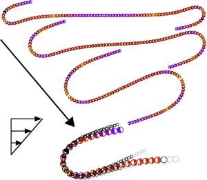
  $\dot{\gamma}$ is the shear rate, is a nonlinear problem and many approaches have been devised to study it theoretically and numerically, e.g. bead-spring models (Warner Reference Warner1972; Larson et al. Reference Larson, Hu, Smith and Chu1999; Kuei et al. Reference Kuei, Słowicka, Ekiel-Jeżewska, Wajnryb and Stone2015; Słowicka et al. Reference Słowicka, Wajnryb and Ekiel-Jeżewska2015, Reference Słowicka, Stone and Ekiel-Jeżewska2020), cylinder-hinge models (Schmid & Klingenberg Reference Schmid and Klingenberg2000; Férec et al. Reference Férec, Ausias, Heuzey and Carreau2009), slender-body and inextensible Euler–Bernoulli beam (elastica) approaches (Becker & Shelley Reference Becker and Shelley2001; Tornberg & Shelley Reference Tornberg and Shelley2004; Nazockdast et al. Reference Nazockdast, Rahimian, Zorin and Shelley2017; Liu et al. Reference Liu, Chakrabarti, Saintillan, Lindner and Du Roure2018), the boundary integral technique (Peskin Reference Peskin2002), the method of regularized Stokeslets (Cortez, Fauci & Medovikov Reference Cortez, Fauci and Medovikov2005; Nguyen & Fauci Reference Nguyen and Fauci2014; LaGrone et al. Reference LaGrone, Cortez, Yan and Fauci2019), etc. We exploit the bead-spring approach for numerical simulations and the elastica model for rationalization of the numerical results (see figure 1).

Figure 1. Models of a fibre in shear flow and the notation. (a) The bead model. (b) The elastica model.
2.1. Bead model
The bead-spring model illustrated in figure 1(a) describes elastic and hydrodynamic interactions between  $n$ numbered $i = 1,\ldots ,n$ spherical beads of identical radii $a$ (
$a$ ( $i$th bead position is denoted as $\boldsymbol {R}_i$). In this work, we use three different bead models $\mathcal {M}_i,\ i=1,2,3$ (cf. table 1), which include combinations of two different descriptions of hydrodynamic interactions (HI), described below and in appendix A: the generalized Rotne–Prager–Yamakawa (GRPY) method (Wajnryb et al. Reference Wajnryb, Mizerski, Zuk and Szymczak2013; Zuk et al. Reference Zuk, Cichocki and Szymczak2017) and the multipole method with lubrication correction (Hydromultipole) (Cichocki, Ekiel-Jeżewska & Wajnryb Reference Cichocki, Ekiel-Jeżewska and Wajnryb1999; Ekiel-Jeżewska & Wajnryb Reference Ekiel-Jeżewska and Wajnryb2009) with two sets of constitutive laws specifying elastic interactions that are described next.
Table 1. Physical assumptions of the bead-spring models  $\mathcal {M}_1$, $\mathcal {M}_2$ and $\mathcal {M}_3$.

The results presented in the following sections are based on the numerical simulations from the bead models  $\mathcal {M}_1$ and $\mathcal {M}_2$. Both of them have the same long-distance asymptotics of the hydrodynamic interactions, and for close beads the Hydromultipole method is more precise than the GRPY. However, the computations based on the Hydromultipole algorithm require more time and memory than the GRPY approach. The GRPY model has been therefore used in simulations of very long fibres. For $n\le 100$ both $\mathcal {M}_1$ and $\mathcal {M}_2$ have been applied.
Qualitative results from the bead-spring models  $\mathcal {M}_1$ and $\mathcal {M}_2$ are similar and in regimes of large $A$ and $n$ they are also the same quantitatively. A detailed comparison of the results obtained within both models is given in appendix B. The model $\mathcal {M}_3$ (see table 1) is applied there to explain that some differences between the models $\mathcal {M}_1$ and $\mathcal {M}_2$ are related to different expressions for the bending potential energy, in agreement with the predictions of Bukowicki & Ekiel-Jeżewska (Reference Bukowicki and Ekiel-Jeżewska2018).
2.1.1. Elastic interactions
An elastic interaction potential model (constitutive laws) specifies a sum  $\mathcal {E}$ of all bead–bead interaction energies, which are used to calculate elastic forces $\boldsymbol {F}_i=-\boldsymbol {\nabla }_{\boldsymbol {R}_i} \mathcal {E}$ acting on each bead $i$. We assume that there are no elastic torques acting on the beads. For every pair of beads $i,j$ the connector vector $\boldsymbol {R}_{ij}=\boldsymbol {R}_j-\boldsymbol {R}_i$ points from the centre of the sphere $i$ towards the centre of sphere $j$.
$j$.
For the first set of constitutive laws, set 1, between the centres of every two consecutive beads  $i$ and $i+1$ we impose the FENE (finitely extensible nonlinear elastic) stretching potential energy (Warner Reference Warner1972)
 \begin{equation} E_{s,ij} = \frac{k'_s R_m^2}{2}\log \left[ 1 - \left(\frac{R_{ij}-2a}{R_m}\right)^2 \right],\end{equation}
where  $j=i+1$, $k'_s$ is the spring stiffness, $R_m=0.2a$ is the maximum stretching from the equilibrium distance and $R_{ij}=|{\boldsymbol {R}}_{ij}|$. Between every triplet of beads $i-1,i,i+1$ we impose a harmonic bending potential energy,
 \begin{equation} E_{b,i} = \frac{A'}{2} (\theta_0 - \theta_i)^2,\end{equation}
where  $\theta _i$ and $\theta _0$ are, respectively, the time-dependent and the equilibrium angles between connector vectors $\boldsymbol {R}_{i,i-1}$ and $\boldsymbol {R}_{i,i+1}$, and $A'=EI/L_0$ is the bending stiffness (per unit length), with the Young modulus $E$, the moment of inertia $I={\rm \pi} a^4/4$ and the distance $L_0$ between the centres of the consecutive beads. Because a fibre is straight, when in equilibrium, the angle $\theta _0={\rm \pi}$. In the set 1 of the constitutive laws we assume that $L_0=2a$.
For the second set of constitutive laws, set 2, between centres of every two consecutive beads  $i$ and $i+1$ we impose a harmonic stretching potential energy
 \begin{equation} E_{s,ij} = \frac{k'_s}{2} (R_{ij}-L_0)^2,\end{equation}
with  $j=i+1$ and the equilibrium distance $L_0$ between the bead centres usually close to $R_0=2a$ but a bit larger. Between every triplet of beads $i-1,i,i+1$ we impose a cosine (Kratky–Porod) bending potential energy
 \begin{equation} E_{b,i} = A' \left(1 + \frac{\boldsymbol{R}_{i,i-1}\boldsymbol{\cdot} \boldsymbol{R}_{i,i+i}}{|\boldsymbol{R}_{i,i-1}||\boldsymbol{R}_{i,i+i}|}\right) = A' (1 + \cos\theta_i ). \end{equation}
This potential energy is a widely used discrete approximation of the elastic bending stiffness, see e.g. Gauger & Stark (Reference Gauger and Stark2006).
Additionally when the GRPY model of hydrodynamic interactions is used we add the repulsive part of the Lennard-Jones potential energy
 \begin{equation} E_{R,ij} = 4 \epsilon'_{LJ} \left( \frac{\sigma_{LJ}}{R_{ij}} \right)^{12}\end{equation}
between the second nearest or further neighbour beads, where  $\epsilon '_{LJ}$ determines the strength of the potential and $\sigma _{LJ}$ is the characteristic distance. We set $\sigma _{LJ}=2a$ and truncate the Lennard-Jones interaction range to $2.5 \sigma _{LJ}$. This potential acts to prevent large overlaps of the beads (comparable with $2a - R_{ij} \ll a$ for $R_{ij}<2a$). This is not necessary for the Hydromultipole model because the lubrication forces prevent the beads from overlapping.
2.1.2. Hydrodynamic interactions
In this work, we study translational motion of segments of a flexible fibre. In the framework of the bead-spring modelling, the translational motion of the fibre beads is determined by the theory of hydrodynamic interactions between spherical particles. We consider  $n$ spherical particles in a fluid of viscosity $\mu _0$ subject to an incompressible external flow $\boldsymbol {V}_{\infty }(\boldsymbol{R})$. We investigate the case where the Reynolds number is much smaller than unity and the quasi-steady fluid velocity $\boldsymbol {V}(\boldsymbol {R})$ and pressure $p(\boldsymbol {R})$ are described by the Stokes equations (Oseen Reference Oseen1927; Kim & Karrila Reference Kim and Karrila1991).
The theory of hydrodynamic interactions is used to calculate the translational velocities  $\boldsymbol {U}_i$ of the particles, which are in turn necessary to integrate the particle trajectories. In our case the external flows are linear, and there are no torques applied to the particles. Therefore the translational velocities $\boldsymbol {U}_{i}$ satisfy the relations,
 \begin{equation} \boldsymbol{U}_{i} = \boldsymbol{V}_{\infty}(\boldsymbol{R}_i) + \sum_{j=1}^n \left(\boldsymbol{\mu}^{tt}_{ij} \boldsymbol{\cdot} \boldsymbol{F}_j + \boldsymbol{\mu}^{td}_{ij} : \boldsymbol{E}_{\infty}\right), \end{equation}
where  $\boldsymbol {F}_j$ is the total external force exerted on the particle $j$ and $\boldsymbol {E}_{\infty }=(\boldsymbol {\nabla } \boldsymbol {V}_{\infty }+ (\boldsymbol {\nabla } \boldsymbol {V}_{\infty })^{\textrm {T}})/2$ denotes the rate-of-strain tensor of the external fluid flow $\boldsymbol {V}_{\infty }$. For the shear flow given by (2.1),
 \begin{equation} \boldsymbol{E}_{\infty} = \frac{\dot{\gamma}}{2}\left(\begin{array}{@{}ccc@{}} 0 & 0 & 1 \\ 0 & 0 & 0 \\ 1 & 0 & 0 \end{array}\right). \end{equation}
 There are different methods to evaluate the translational–translational  $\boldsymbol {\mu }^{tt}_{ij}$ and translational–dipolar $\boldsymbol {\mu }^{td}_{ij}$ mobility matrices. The most precise is the multipole expansion, corrected for lubrication, in order to speed up the convergence (Durlofsky, Brady & Bossis Reference Durlofsky, Brady and Bossis1987; Cichocki et al. Reference Cichocki, Felderhof, Hinsen, Wajnryb and Bławzdziewicz1994; Sangani & Mo Reference Sangani and Mo1994; Cichocki et al. Reference Cichocki, Ekiel-Jeżewska and Wajnryb1999; Ekiel-Jeżewska & Wajnryb Reference Ekiel-Jeżewska and Wajnryb2009) through the inverse-power expansion in the inter-particle distance (Kim & Karrila Reference Kim and Karrila1991). The analytical Rotne–Prager–Yamakawa approximation is also often used (Rotne & Prager Reference Rotne and Prager1969).
In this work we evaluate the mobility matrices as functions of the positions of all the beads using the two methods outlined in appendix A. First, we apply the analytical Rotne–Prager–Yamakawa approximation of the translational–translational mobility  $\boldsymbol {\mu }^{tt}_{ij}$ (Rotne & Prager Reference Rotne and Prager1969), generalized also for the translational–dipolar mobility matrix $\boldsymbol {\mu }^{td}_{ij}$ (Kim & Karrila Reference Kim and Karrila1991) and implemented in the GRPY numerical program. Second, we use the precise multipole method corrected for lubrication, implemented in the numerical code Hydromultipole. The GRPY procedure is less precise, when particle surfaces are closer than the radius of the smaller particle, but computationally much faster than the Hydromultipole algorithm. Both methods will be briefly outlined in appendix A.
The equations of motion for the positions  $\boldsymbol {R}_i$ of the beads are
 \begin{equation} \dot{\boldsymbol{R}}_{i} = \boldsymbol{U}_{i}, \end{equation}
with  $\boldsymbol {U}_i$ dependent on the positions $\boldsymbol {R}_{j}$ of all the bead centres $j=1,\ldots ,n$, and given by (2.7).
The equations of motion (2.9) are solved numerically with the use of dimensionless variables. We choose as a characteristic length the bead diameter  $2a$. The total length of the fibre at equilibrium is $L$, which in the case of the $\mathcal {M}_1$ model is fixed to $L=2na$ so that the fibre aspect ratio is $n$. We choose as a time scale the inverse of the shear rate $\dot {\gamma }^{-1}$ and the forces are normalized with ${\rm \pi} \mu _0 \dot {\gamma } (2a)^2$. The above introduces the dimensionless stretching stiffness $k_s=k'_s/({\rm \pi} \mu _0 \dot {\gamma } (2a))$, $\epsilon _{LJ}=\epsilon '_{LJ}/({\rm \pi} \mu _0 \dot {\gamma } (2a)^3)$ and the bending stiffness
 \begin{equation} A=A'/({\rm \pi} \mu_0 \dot{\gamma} (2a)^3)=EI/({\rm \pi} \mu_0 \dot{\gamma} L_0 (2a)^3). \end{equation}
For the GRPY approach,  $L_0=2a$. Note that for the Hydromultipole treatment of the hydrodynamic interactions, the dimensionless bending stiffness ratio $A$ used here is slightly different from the corresponding parameter $EI/({\rm \pi} \mu _0 \dot {\gamma } (2a)^4)$ used by Słowicka et al. (Reference Słowicka, Wajnryb and Ekiel-Jeżewska2013, Reference Słowicka, Wajnryb and Ekiel-Jeżewska2015, Reference Słowicka, Stone and Ekiel-Jeżewska2020) and denoted there by the same letter. To adjust for this difference, all the numerical values of the bending stiffness based on the Hydromultipole codes taken from earlier works were in this paper divided by $L_0/(2a)$ (typically equal to 1.02 or 1.01, see appendix B).
2.1.3. Why a fibre aligned with the flow moves out of this position
To answer this question, we will use (2.7) to analyse the velocities of the beads for a fibre aligned with the flow and at the elastic equilibrium. We will use the standard pairwise-additive Rotne–Prager–Yamakawa (RPY) approximation for the distinct mobility matrices  $\boldsymbol {\mu }^{tt}_{ij}$ and $\boldsymbol {\mu }^{td}_{ij}$ with $i \ne j$ (Kim & Karrila Reference Kim and Karrila1991). From the geometric symmetry we can write down the tensorial form of the mobility matrices for a pair of particles $i$ and $j$ (Kim & Karrila Reference Kim and Karrila1991),
 \begin{gather} \boldsymbol{\mu}^{tt}_{ij} = A (R_{ij}) \boldsymbol{d}_{ij} \boldsymbol{d}_{ij} + B (R_{ij}) (\boldsymbol{I} - \boldsymbol{d}_{ij}\boldsymbol{d}_{ij}), \end{gather}
 \begin{gather}\boldsymbol{\mu}^{td}_{ij} = C (R_{ij}) \big( \boldsymbol{d}_{ij} \boldsymbol{d}_{ij} - \tfrac{1}{3}\boldsymbol{I} \big) \boldsymbol{d}_{ij} + D (R_{ij}) \overline{\boldsymbol{d}_{ij}(\boldsymbol{I}-\boldsymbol{d}_{ij}\boldsymbol{d}_{ij})}, \end{gather}
where  $\boldsymbol {I}$ is the unit tensor, $\boldsymbol {d}_{ij} = \boldsymbol {R}_{ij}/|\boldsymbol {R}_{ij}|$, and $\overline {\boldsymbol {d}_{ij}(\boldsymbol {I}-\boldsymbol {d}_{ij}\boldsymbol {d}_{ij})}$ is a third rank tensor symmetric and traceless in the first and second Cartesian components, i.e. $\overline {\boldsymbol {d}_{ij} (\boldsymbol {I}-\boldsymbol {d}_{ij}\boldsymbol {d}_{ij})} _{\alpha \beta \gamma } = \frac {1}{2}( d_\alpha \delta _{\beta \gamma } + d_\beta \delta _{\alpha \gamma })-d_\alpha d_\beta d_\gamma$, where the Cartesian components are labelled with the Greek letters. Within the RPY approximation, the translational– translational self-mobility matrix
 \begin{equation} \boldsymbol{\mu}^{tt}_{ii}=\frac{1}{6 {\rm \pi}\mu_0 a} {\boldsymbol I}\end{equation}
and the translational–dipolar self-mobility matrix vanishes,  $\boldsymbol {\mu }^{td}_{ii}=\boldsymbol {0}$.
Our goal now is to investigate the initial configuration, when the fibre is parallel to the flow. In this case  $\boldsymbol {d}_{ij} = \pm \hat {\boldsymbol {e}}_x$, with the minus sign for the beads with labels $i>j$. Since the fibre is at the elastic equilibrium, the external forces vanish, $\boldsymbol {F}_j=\boldsymbol {0}$, and the only contribution to velocity in the direction perpendicular to the flow comes from the translational–dipolar mobility. From (2.11b) it follows that the contribution to the velocity $\boldsymbol {U}_{i}$ of particle $i$ from the translational–dipolar mobility $\boldsymbol {\mu }^{td}_{ij}$ acting on the strain tensor $\boldsymbol {E}_{\infty }$ (where $[\boldsymbol {A}:\boldsymbol {B}]_{ij} = A_{ik} B_{kj}$) consists of two terms proportional to
 \begin{align} \left(\boldsymbol{d}_{ij} \boldsymbol{d}_{ij}-\frac{1}{3}\boldsymbol{I}\right) \boldsymbol{d}_{ij}: \boldsymbol{E}_{\infty} = \frac{\dot{\gamma}}{2}\left(\begin{array}{c} 0 \\ 0 \\ 1/3 \end{array}\right)\quad \mbox{and}\quad \overline{\boldsymbol{d}_{ij} (\boldsymbol{I} -\boldsymbol{d}_{ij} \boldsymbol{d}_{ij})}: \boldsymbol{E}_{\infty}= \frac{\dot{\gamma}}{2} \left(\begin{array}{c} 0 \\ 0 \\ -1 \end{array}\right), \end{align}
respectively. Therefore, there exist contributions to the bead velocities perpendicular to the flow, and this is why the fibre moves out of the position aligned with the flow. In the next section, we will show that the largest are perpendicular velocities of the first and last beads, at the initial configuration aligned with the flow, and also later when the fibre is slightly deflected. We will also demonstrate that this effect can be considered as the result of a hydrodynamic force exerted by the shear flow on the fibre.
2.1.4. Hydrodynamic force acting on the tip of the fibre initially aligned with the flow
We now move on to the discussion of the hydrodynamic force exerted by the shear flow on the tip of a fibre aligned with the flow or already slightly deflected from the alignment. In the following, we are going to provide the theoretical explanation for the initial stage of the bending process in terms of the elastica, based on the assumption that a constant hydrodynamic force is exerted on the fibre end by the shear flow. In the standard use of the elastica equations the existence of such a force has not been yet taken into account. Here, we use the general framework of the theory of hydrodynamic interactions presented in the previous sections to explain the physical origin of this force, and to estimate its value numerically (with the bead model  $\mathcal {M}_1$).
In the bead models, the tip force can be found rewriting (2.7)
 \begin{equation} \dot{\boldsymbol{R}}_i - \boldsymbol{V}_{\infty}(\boldsymbol{R}_i) = \boldsymbol{\mu}^{tt}_{ii} \boldsymbol{\cdot} \left( \boldsymbol{F}_i + (\boldsymbol{\mu}^{tt}_{ii})^{-1} \sum_{j} \boldsymbol{\mu}^{td}_{ij} : \boldsymbol{E}_{\infty}\right)+\sum_{j \neq i} \left(\boldsymbol{\mu}^{tt}_{ij} \boldsymbol{\cdot} \boldsymbol{F}_j\right), \end{equation}
where  $\boldsymbol {\mu }^{tt}_{ii}$ is the translational self-mobility matrix, and defining the hydrodynamic force acting on bead $i$ as
 \begin{equation} \boldsymbol{F}_{Hi} = (\boldsymbol{\mu}^{tt}_{ii})^{-1} \sum_{j} \boldsymbol{\mu}^{td}_{ij} : \boldsymbol{E}_{\infty}. \end{equation}
The dimensionless form is  $\boldsymbol {f}_{Hi}=\boldsymbol {F}_{Hi}/( {\rm \pi}\mu _0 \dot {\gamma } (2a)^2 )$.
Our goal is to investigate  ${\boldsymbol F}_{Hi}$ at the early stage of the evolution, when the fibre, initially aligned with the flow, slowly moves out of this configuration, but still remains almost parallel to the flow. We will now show that, for the fibre almost aligned with the flow, the hydrodynamic forces $\boldsymbol {F}_{Hi}$, defined by (2.15), are almost perpendicular to the flow direction $\hat {\boldsymbol {e}}_x$. We will also provide some theoretical arguments why the value of ${\boldsymbol F}_{Hi}$ is the largest at the ends of the fibre.
The hydrodynamic forces  ${\boldsymbol F}_{Hi}$ given by (2.15) are proportional to the shear rate $\dot {\gamma }$. Moreover, the force $\boldsymbol {F}_{Hi}$ is perpendicular to the flow and parallel to the $z$ direction of the flow gradient, ${\boldsymbol F}_{Hi} \approx \hat {\boldsymbol e}_z \boldsymbol{\cdot} {\boldsymbol F}_{Hi} \hat {\boldsymbol e}_z$. Therefore, they displace the fibre beads away from the position aligned with the flow. From the explicit expressions for the functions $C$ and $D$ in (2.11b), given e.g. by Kim & Karrila (Reference Kim and Karrila1991), it follows that for the first bead $\hat {\boldsymbol e}_z \boldsymbol{\cdot} {\boldsymbol F}_{H1} > 0$ and for the last bead $\hat {\boldsymbol e}_z \boldsymbol{\cdot} {\boldsymbol F}_{Hn} < 0$. This means that, owing to the hydrodynamic forces (2.15), the fibre follows the rotational component of the shear flow.
It is also known that  $C \propto R_{ij}^{-2}$ and $D\propto R_{ij}^{-4}$, see e.g. Kim & Karrila (Reference Kim and Karrila1991). Therefore, the major contribution to $F_{Hi}$ comes from relatively close beads $j$. Additionally, $\boldsymbol {\mu }^{td}_{ij}$ is antisymmetric in $\boldsymbol {d}_{ij}$, which means that the terms in (2.15) corresponding to equally distant left and right neighbours will cancel. Therefore, the total force $F_{Hi}$ is close to zero for $i$ in the middle part of the fibre, and it increases when $i$ is closer to the fibre ends. For longer fibres, the force $F_{Hi}$ is non-negligible only for $i$ close to one of the fibre ends, and it only weakly depends on the total fibre length because it comes from unbalanced local interactions between the bead $i$ and close beads $j$.
$j$.
To evaluate  $\boldsymbol {f}_{Hi}$ numerically, we use the pairwise-additive GRPY approximation for the mobility matrices. As argued above, in the stage when fibre is only slightly deflected from the straight line, at leading order, $\boldsymbol {f}_{Hi}$ is directed along $\hat {\boldsymbol {e}}_z$. In figure 2(a) we plot the dimensionless hydrodynamic force $\hat {\boldsymbol {e}}_{z} \boldsymbol{\cdot} \boldsymbol {f}_{Hi}$ as a function of the bead label $i$ for three different fibre lengths $n$. It is clear that the force is well localized close to the fibre ends.

Figure 2. Hydrodynamic forces normal to the fibre, acting on bead  $i$, calculated from (2.15) with the GRPY model of the hydrodynamic interactions. (a) Spatial distribution of the forces on the beads along the fibre. (b) The force on the first bead as a function of the fibre aspect ratio $n$.
$n$.
The orientation of  $\boldsymbol {f}_{Hi}$ follows the rotational component of the shear flow. As the fibre gets longer, the force is more localized. Regardless of the fibre length, the end beads support the largest forces, an order of magnitude larger than the forces acting on the other beads. The magnitude of the force acting on the first bead, $\boldsymbol {f}_{H1} \boldsymbol{\cdot} \hat {\boldsymbol {e}}_z$, initially changes non-monotonically as a function of $n$ (see figure 2b), until it reaches a limiting value $\,f_H \approx 0.16$. Indeed, we observe a localized, length-independent tip force perpendicular to the flow. We will use this observation later to construct a modified elastica model, applicable for a fibre initially aligned with the flow. Now it is time to present the standard Euler–Bernoulli beam, based on the local slender-body theory.
2.2. The elastica and local slender-body theory
To rationalize the results of numerical simulations from the bead-spring simulations the inextensible elastica model (Duprat & Stone Reference Duprat and Stone2015; Lindner & Shelley Reference Lindner and Shelley2015) is used with the local slender-body theory (SBT) (Cox Reference Cox1970; Keller & Rubinow Reference Keller and Rubinow1976; Johnson Reference Johnson1980) to account for the drag forces acting along the fibre. Within the local SBT, in contrast to the bead models, the full long-ranged hydrodynamic interactions are not incorporated, nor is the finite but small thickness of the filament. The last feature is especially important for fibres that are aligned with the flow, as will be discussed in detail later. Similarly as in the bead model, for the elastica we also neglect Brownian motion and buoyancy forces. The fibre has a circular cross-section of radius  $a$ and length $L=2na$ where $\epsilon = {a}/{L} = {1}/{2n} \ll 1$. We denote as $\boldsymbol {R}(S,T)$ the dimensional position of a fibre segment at the arc length $S$ at time $T$. The equation of motion of each filament segment as a result of the applied elastic force density $\boldsymbol {F}(S,T)$ per unit length, under the steady undisturbed flow $\boldsymbol {V}_{\infty }$ can be expressed using the SBT (Cox Reference Cox1970; Duprat & Stone Reference Duprat and Stone2015; Lindner & Shelley Reference Lindner and Shelley2015)
 \begin{equation} \dot{\boldsymbol{R}} - \boldsymbol{V}_{\infty}(\boldsymbol{R}) = \frac{\ln(\epsilon^{-1})}{4 {\rm \pi}\mu_0} \left( \boldsymbol{I} + \boldsymbol{R}_S \boldsymbol{R}_S \right) \boldsymbol{\cdot} \boldsymbol{F}(S,T), \end{equation}
or alternatively
 \begin{equation} \frac{2 {\rm \pi}\mu_0}{\ln(\epsilon^{-1})} ( 2 \boldsymbol{I} - \boldsymbol{R}_S \boldsymbol{R}_S ) \boldsymbol{\cdot} ( \dot{\boldsymbol{R}} - \boldsymbol{V}_{\infty}(\boldsymbol{R}) ) = \boldsymbol{F}(S,T), \end{equation}
where  $\dot {\boldsymbol {R}}={\partial \boldsymbol {R}}/{\partial T}$, $\boldsymbol {R}_S = {\partial \boldsymbol {R}}/{\partial S}$ and the relative motion of the filament is obtained by applying the mobility tensor, proportional to the anisotropic tensor $( \boldsymbol {I} + \boldsymbol {R}_S \boldsymbol {R}_S )$, to the elastic force $\boldsymbol {F}(S,T)$ on the fibre. Here, we consider shear flow $\boldsymbol {V}_{\infty }(\boldsymbol {R}) = \dot {\gamma } \text {Z} \hat {\boldsymbol {e}}_x$, where $\text {Z}=\hat {\boldsymbol {e}}_z \boldsymbol{\cdot} \boldsymbol {R}$. For the elastic fibre we use the notation illustrated in figure 1(b), i.e. $\hat {\boldsymbol {e}}_n$ denotes a unit vector normal to the fibre in the shear plane and $\hat {\boldsymbol {e}}_s$ denotes a unit vector tangent to the fibre. The inextensibility condition $|\boldsymbol {R}_S|=1$ results in $\hat {\boldsymbol {e}}_s = \boldsymbol {R}_S$ and implies the Frenet formulas ${\partial \hat {\boldsymbol {e}}_{s}}/{\partial S} = K \hat {\boldsymbol {e}}_n,\ {\partial \hat {\boldsymbol {e}}_{n}}/{\partial S} = - K \hat {\boldsymbol {e}}_s$, where $K$ is the local curvature and we have assumed that the fibre shape is planar.
In the elastica model the elastic forces acting on the unit segment of the fibre are (Audoly & Pomeau Reference Audoly and Pomeau2000; Audoly Reference Audoly2015)
 \begin{equation} \boldsymbol{F}(S,T) =( - E I K_S \hat{\boldsymbol{e}}_n+ \varSigma \hat{\boldsymbol{e}}_s)_S, \end{equation}
where  $\varSigma (S,T)$ is the tension in the filament (satisfying inextensibility), $E$ is the Young modulus and $I$ is the moment of inertia ( $I={\rm \pi} a^4 /4$), as earlier. Alternatively, the force density per unit length can be expressed as $\boldsymbol {F}(S,T) = - EI {\boldsymbol R}_{SSSS} + (\mathcal {T} \hat {\boldsymbol {e}}_s)_S$, see e.g. Tornberg & Shelley (Reference Tornberg and Shelley2004) and Lindner & Shelley (Reference Lindner and Shelley2015). It is easy to check that $\varSigma = \mathcal {T}+EIK^2$.
With the use of the Frenet formulas it is convenient to write separately the equations of motion in the normal and tangential directions, respectively,
 \begin{gather} \frac{4 {\rm \pi}\mu_0}{\ln(\epsilon^{-1})} \hat{\boldsymbol{e}}_n \boldsymbol{\cdot} ( \dot{\boldsymbol{R}} -\dot{\gamma} \hat{\boldsymbol{e}}_x (\hat{\boldsymbol{e}}_z \boldsymbol{\cdot} \boldsymbol{R}) ) = - E I K_{SS} + \varSigma K, \end{gather}
 \begin{gather}\frac{2 {\rm \pi}\mu_0}{\ln(\epsilon^{-1})} \hat{\boldsymbol{e}}_s \boldsymbol{\cdot} ( \dot{\boldsymbol{R}} - \dot{\gamma} \hat{\boldsymbol{e}}_x (\hat{\boldsymbol{e}}_z \boldsymbol{\cdot} \boldsymbol{R}) ) = \left( \varSigma + \frac{E I}{2} K^2 \right)_{S}. \end{gather}
We write the dimensionless form (lowercase symbols) of (2.19) by expressing length in the units of  $2a$ and time in the units $\dot {\gamma }^{-1}$, as in § 2.1, to find
 \begin{gather} \eta \hat{\boldsymbol{e}}_n \boldsymbol{\cdot} ( \dot{\boldsymbol{r}} - \hat{\boldsymbol{e}}_x (\hat{\boldsymbol{e}}_z \boldsymbol{\cdot} \boldsymbol{r}) ) = - \kappa_{ss} + \sigma \kappa, \end{gather}
 \begin{gather}\frac{\eta}{2} \hat{\boldsymbol{e}}_s \boldsymbol{\cdot} ( \dot{\boldsymbol{r}} - \hat{\boldsymbol{e}}_x (\hat{\boldsymbol{e}}_z \boldsymbol{\cdot} \boldsymbol{r}) ) = \left( \sigma + \frac{1}{2} \kappa^2 \right)_s, \end{gather}
where
 \begin{equation} \eta=\frac{4 {\rm \pi}\mu_0 (2a)^4 \dot{\gamma}}{E I \ln(\epsilon^{-1})}\end{equation}
is a dimensionless compliance. Using the same normalization of  $EI$ as for the bead model, $EI/({\rm \pi} \mu _0 \dot {\gamma } L_0 (2a)^3)$, we can formally write $\eta = {4(2a)}/{A L_0\ln (\epsilon ^{-1})}$. A physical comparison between the elastica and bead models will be presented in § 4.3.
The dimensionless compliance  $\eta$ is very similar to the elasto-viscous number $\bar {\eta }={8 {\rm \pi}\mu _0 L^4 \dot {\gamma }}/{E I \ln (\epsilon ^{-1})}$ (Becker & Shelley Reference Becker and Shelley2001; Tornberg & Shelley Reference Tornberg and Shelley2004; Wandersman et al. Reference Wandersman, Quennouz, Fermigier, Lindner and Du Roure2010; Nguyen & Fauci Reference Nguyen and Fauci2014; Liu et al. Reference Liu, Chakrabarti, Saintillan, Lindner and Du Roure2018; LaGrone et al. Reference LaGrone, Cortez, Yan and Fauci2019; du Roure et al. Reference du Roure, Lindner, Nazockdast and Shelley2019). The main difference is that $\bar {\eta }$ has the fibre's length $L$ as the typical length scale, while $\eta$ uses the fibre's radius.
3. A typical bead model simulation
The dimensionless stretching stiffness is fixed to a large value ( $k_s=2000$ in the $\mathcal {M}_1$ model and $k_s=1000$ in the $\mathcal {M}_2$ model) so that the fibre is close to inextensible. In $\mathcal {M}_1$, the equilibrium distance between the bead centres corresponds to the touching beads, $L_0=2a$ and the dimensionless Lennard-Jones potential coefficient $\epsilon _{LJ}=5$ allows only slight overlaps. In $\mathcal {M}_2$, lubrication interactions between close particle surfaces prevent overlaps. The equilibrium distance $L_0$ between the bead centres has to be a bit larger than the bead diameter $2a$; here we choose $L_0/(2a)=1.02$. Sensitivity of the ${\mathcal {M}}_2$ model to the choice of $L_0$ has been discussed by Słowicka et al. (Reference Słowicka, Wajnryb and Ekiel-Jeżewska2015, Reference Słowicka, Stone and Ekiel-Jeżewska2020).
We focus on the fibre dynamics under the influence of the dimensionless bending stiffness  $A$ and the number of beads $n$, indicating the fibre's aspect ratio. The typical shape of a fibre during the evolution is presented in figure 3(a).The simulations (based on the $\mathcal {M}_1$ model) start from a stretched fibre aligned in the flow direction. First, we observe a slow deflection of the fibre tips up to time approximately 30. Later, until the time 35, rapid bending of the tip occurs. Next, a curling motion appears, with the maximum curvature moving to the central part of the fibre, and a typical shape is shown for $t=47$. After the kinked parts of the fibre pass over each other (around time 62), the fibre rapidly straightens to a position slightly tilted from the $x$ direction at time 66, after which the fibre slowly stretches and aligns in the $x$ direction until the end beads reach the same $z$ coordinate at time 141.

Figure 3. A typical evolution of the shape of a flexible fibre with aspect ratio  $n=100$ and a moderate bending stiffness $A=100$ (based on the model $\mathcal {M}_1$), starting from a straight fibre aligned with the flow. (a) Shapes of the fibre. The circles represent the beads actual scale along the fibre. The black circles highlight the end and middle beads during $\tau _f$ and $\tau _m$. (b) Maximum local curvature $\kappa (t)$. Time instances corresponding to the shapes from (a) are marked with dashed vertical lines.
To characterize the deformation of a fibre, an informative observable is the maximum local curvature  $\kappa (t)$ taken over the fibre length at every time instant, where, similarly to the elastica model, we use lowercase symbols for the dimensionless quantities (see § 2.1). At every time $t$ we inscribe a circle of radius $r_{i-1,i,i+1}(t)$ on the bead centres $\boldsymbol {r}_{i-1},\boldsymbol {r}_i,\boldsymbol {r}_{i+1}$, defining the local curvature $\kappa _{i}(t)=1/r_{i-1,i,i+1}(t)$. The maximum local curvature is defined as
 \begin{equation} \kappa(t) = \max_{ 2 \le i \le n-1} \kappa_{i}(t).\end{equation}
A typical profile of  $\kappa (t)$ obtained from the simulations is shown in figure 3(b). We identify two characteristic bending curvatures $\kappa _{b1}$, the value of the first plateau, and $\kappa _{b2}$, the maximum value over time. To characterize the shape changes, we introduce characteristic time scales: $\tau _b$, the bending time, then $\tau _c$, the curling time, and $\tau _s$, the stretching time, as indicated in figure 3.
Initially, for an almost straight fibre,  $\kappa (t)$ is close to 0. The rapid rise in curvature (starting around $t=30$) is connected with rapid bending of the ends until a characteristic curvature $\kappa _{b1}$ is reached. We define the time scale $\tau _b$ as the time needed for a fibre to reach half of its maximum curvature $\kappa _{b2}$ starting from a straight fibre.
After the rapid bending, a curling motion occurs. We observe the end beads passing above each other (having the same  $x$ coordinate) at a flipping time $\tau _f=47$ ( $\tau _f$ was called the flipping time by Słowicka et al. (Reference Słowicka, Wajnryb and Ekiel-Jeżewska2013, Reference Słowicka, Wajnryb and Ekiel-Jeżewska2015) and is used there to characterize the tumbling dynamics in shear and Poiseuille flows), then the kinks visible in figure 3(a) pass each other. We identify that the last event happens approximately at time $\tau _{b2}=61.4$, when the curvature increases to a maximum value $\kappa _{b2}$. Next, there is a rapid decrease of the fibre curvature. In particular, at a turning time $\tau _m=62.8$ the middle beads have the same $x$ coordinate. Later, we observe a rapid relaxation to an almost straight fibre (here at $t=66$). We define time scale $\tau _c$ as the time from the moment $\tau _b$ when fibre reaches $\kappa _{b2}/2$ for the first time until it reaches $\kappa _{b2}/2$ again after passing the peak of curvature $\kappa _{b2}$.
After rapid relaxation, the fibre is close to straight but tilted from the flow direction. The stretching time scale  $\tau _s$ is evaluated from the time of passing $\kappa _{b2}/2$ for the second time until the fibre ends are aligned with the flow direction again (here at time 141). Then, the motion approximately repeats itself periodically although small changes in the times identified in figure 3 are possible. Therefore, the sum $\tau =\tau _b+\tau _c+\tau _s$ is the tumbling time scale defined as the half-period of the motion and analysed by Słowicka et al. (Reference Słowicka, Wajnryb and Ekiel-Jeżewska2015, Reference Słowicka, Stone and Ekiel-Jeżewska2020), with typically small variations between the first tumbling and the tumblings observed at long times.
With the definitions of  $\tau _b,\tau _c$ and $\tau _s$ we seek to capture the time scales of the slow changes between the (much shorter) steep increase and decrease in curvature, which we consider negligible in comparison to $\tau _b,\tau _c,\tau _s$. Thus, the precise definitions of transitions points between $\tau _b,\tau _c$ and $\tau _s$ can be chosen in a different way and should not have a large influence on the analysis.
We show the changes in the dynamics for different choices of  $n$ and $A$ in figure 4. For a small $A$ and $n$ large enough, the end of the fibre bends multiple times and never returns to the straight state again (figure 4a,b), in which case $\tau _c$ and $\tau _s$ are not defined. Nevertheless $\kappa$ remains approximately constant throughout most of the process. A similar qualitative picture was observed with different experimental (Forgacs & Mason Reference Forgacs and Mason1959b; Harasim et al. Reference Harasim, Wunderlich, Peleg, Kröger and Bausch2013; Liu et al. Reference Liu, Chakrabarti, Saintillan, Lindner and Du Roure2018) and numerical (Lindström & Uesaka Reference Lindström and Uesaka2007; Nguyen & Fauci Reference Nguyen and Fauci2014; Liu et al. Reference Liu, Chakrabarti, Saintillan, Lindner and Du Roure2018; LaGrone et al. Reference LaGrone, Cortez, Yan and Fauci2019) methods. The other limit is when, for a small $n$,
$n$,  $A$ is increased to the point when the fibre bends globally along the whole length.

Figure 4. Differences in the evolution of long, very flexible fibres and short, very stiff fibres (based on the model  $\mathcal {M}_1$). (a) Shapes of a long, flexible fibre with $n=300$, $A=10$. (b) Curvature of the fibre from (a) versus time. The vertical marks correspond to the shapes from panel (a). (c) Shapes of a short, stiff fibre with $n=40$, $A=1000$. (d) Curvature of fibre from (c). The triangle symbols with vertical dashed lines correspond to the times for which the corresponding shapes are shown in panel (c).
In the following, we will first analyse the dynamics for  $0\le t \le \tau _b$ when the bending process originates (§ 4), and next we will study the shape evolution in the time range of large deformation, $\tau _b \le t \le \tau _b+\tau _c$ (§ 5).
4. Bending process of initially straight fibres
4.1. Bending time from numerical simulations
In addition to bending, when in a shear flow, a fibre undergoes rotation (it tumbles). It is instructive to compare the bending time  $\tau _b$, the curling time $\tau _c$ and the stretching time $\tau _s$ (see figure 3) with two indicators of a fibre's rotational motion: the flipping time $\tau _f$ and the turning time $\tau _m$ (see figure 5(a) and the insets indicating shapes for $\tau _f$ and $\tau _m$). We find for $A \in [1,10\,000)$ that $\tau _f < \tau _m$, which shows that the ends of the flexible fibre pass above each other earlier than the middle of the fibre rotates. As $A$ increases, both $\tau _m$ and $\tau _f$ acquire the interpretation of the half-tumbling time $\tau /2$ or the quarter period $T_J/4$ of the Jeffery orbit (Jeffery Reference Jeffery1922), which is understood here as a periodic motion of a certain ‘effective’ rigid elongated object in shear flow (Słowicka et al. Reference Słowicka, Wajnryb and Ekiel-Jeżewska2015, Reference Słowicka, Stone and Ekiel-Jeżewska2020) with the same period $T_J=2\tau$. The period $T_J$ of a Jeffery orbit is approximately proportional to the length of a fibre consisting of $n$ beads (Jeffery Reference Jeffery1922; Kim & Karrila Reference Kim and Karrila1991; Dhont & Briels Reference Dhont and Briels2007; Graham Reference Graham2018).

Figure 5. Characteristic time scales in the fibre motion. (a) Comparison of time scales of the fibre motion: the bending time  $\tau _b$, the stretching time $\tau _s$, the curling time $\tau _c$, the flipping time $\tau _f$ and the turning time $\tau _m$ for $n=60$ and the model $\mathcal {M}_1$. Insets show the shapes for the times $\tau _f$ and $\tau _m$. (b,c) Bending time $\tau _b$ as a function of $A$ for different $n$ from the models $\mathcal {M}_1$ and $\mathcal {M}_2$, respectively. The solid lines show $\tau _b \propto A^{1/3}$. In (b) the best linear fit is $(0.335 \pm 0.002) \log _{10} A + 0.845 \pm 0.005$. (d,e) Bending time $\tau _b$ normalized by $n$ is an almost universal function of $A/n^3$, as confirmed by the numerical data from the models $\mathcal {M}_1$ and $\mathcal {M}_2$, respectively.
For fibres that are very flexible or long enough (e.g.  $A=10$ and $n=300$), $\tau _c$ and $\tau _s$ are not defined, because the fibre does not straighten out again (Słowicka et al. Reference Słowicka, Wajnryb and Ekiel-Jeżewska2015), bending multiple times if $n$ is sufficiently large (figure 4a). In the limit of very stiff fibres, all the time scales defined above, $\tau _b$, $\tau _f$, $\tau _m$ and $\tau _c+\tau _s$, converge to $T_J/4$, as shown in figure 5(a) for large values of $A$. More details about the relation between different time scales can be found in appendix B.
The dynamics of bending changes systematically as a function of  $A$. In figures 5(b) and 5(c) we show $\tau _b$ (see figure 3) as a function of $A$ for different $n$, using the models $\mathcal {M}_1$ and $\mathcal {M}_2$, respectively. Three regimes are visible. First, in the small $A$ regime ( $A \lesssim 10$), the bending dynamics is dominated by large bending angles close to the excluded volume limit. Second, for intermediate $A$,
$A$,  $\tau _b$ does not depend on $n$ and it follows a single power law $\tau _b \propto A^{1/3}$. Third, in the regime of large $A$, the bending time systematically deviates from the power law and saturates at a constant value, where larger $n$ have larger limiting $\tau _b$, in agreement with $\tau _b \rightarrow T_J/4$.
Therefore, in figures 5(d) and 5(e) we replot the data from figures 5(b) and 5(c), respectively, using the rescaled bending time,  $\tau _b/n$. To obtain the universal scaling, we also need to rescale the bending stiffness as $A/n^3$. Indeed, after such rescaling, we observe an almost universal curve in the whole range of values of $n$ and $A$.
$A$.
4.2. A similarity solution at early times for the elastica
In figure 5(b–e) we show the dependence  $\tau _b \propto A^{1/3}$, which can be argued with the help of the elastica model, as we will demonstrate in this and the next section. We observe numerically that, in the power-law regime, the bending time does not depend on the fibre length $n$, which suggests an analysis based on the model of a very long fibre, initially aligned with the flow, with a tip positioned at $S=0$. We assume small deflections from the straight line $\boldsymbol {R} = S \hat {\boldsymbol {e}}_x + U(S,T) \hat {\boldsymbol {e}}_z$, which leads to $K = U_{SS}$. Further, we assume that because of small deflections, $\hat {\boldsymbol {e}}_s = \hat {\boldsymbol {e}}_x$ and $\hat {\boldsymbol {e}}_n = \hat {\boldsymbol {e}}_z$. Under these assumptions, we rewrite the dimensional linearized equations (2.19)
 \begin{gather} \dot{U}(S,T) = - \frac{E I \ln(\epsilon^{-1})}{4 {\rm \pi}\mu_0} U_{SSSS}(S,T) + \frac{\ln(\epsilon^{-1})}{4 {\rm \pi}\mu_0} F_E \delta(S) , \end{gather}
 \begin{gather}U(S,T) = - \frac{\ln(\epsilon^{-1})}{2 {\rm \pi}\mu_0} \varSigma_S(S,T), \end{gather}
with the Dirac delta  $\delta (S)$ in the additional term that introduces the hydrodynamic force $F_E=O(1)$, perpendicular to the fibre axis, acting on the tip of the fibre at $S=0$. This force results from the hydrodynamic interactions of the fibre beads in response to the shear flow (see §§ 4.3 and 2.1.4). Alternatively to the delta term, the constant tip force can be formally written as a boundary condition, $U_{SSS}(S\!=\!0,T)$= $F_E /(E I)$. We will use this approach to write (4.1) in the dimensionless form, corresponding to (2.20),
 \begin{gather} \dot{u} = - \frac{1}{\eta} u_{ssss}, \end{gather}
 \begin{gather}u = - \frac{2}{\eta} \sigma_s. \end{gather}
In order to solve (4.2a) we apply boundary conditions
 \begin{equation} u \left(\infty,t \right) = 0, \quad u_{ss} \left(\infty,t \right) = 0, \quad \frac{1}{\eta} u_{sss}\left( 0, t \right) = \mathcal{F}, \end{equation}
where
 \begin{equation} \mathcal{F}=\frac{\ln(\epsilon^{-1})}{4} \,f_E \end{equation}
with  $\,f_E = F_E / ({\rm \pi} \mu _0 \dot {\gamma } (2a)^2)$. We impose an initial condition
 \begin{equation} u \left(s,t=0 \right) = 0. \end{equation}
We seek a similarity solution (Barenblatt Reference Barenblatt1996; Duprat & Stone Reference Duprat and Stone2015; Eggers & Fontelos Reference Eggers and Fontelos2015) and account for the forcing as
 \begin{equation} u \left( s,t \right) = \eta^{1/4} \mathcal{F} t^{3/4} \mathcal{U} \left( \chi \right),\quad \textrm{where} \ \chi = \eta^{1/4} \frac{s}{t^{1/4}}, \end{equation}
which leads to the equation
 \begin{equation} 4 \mathcal{U}_{\chi\chi\chi\chi} + 3 \mathcal{U} - \chi \mathcal{U}_{\chi} = 0 \end{equation}
with the boundary conditions
 \begin{equation} \mathcal{U} \left( \infty \right) = 0,\quad \mathcal{U}_{\chi\chi} \left( 0 \right) = 0,\quad \mathcal{U}_{\chi\chi\chi} \left( 0 \right) = 1.\end{equation}
The solution can be expressed with the help of special (hypergeometric) functions (e.g. use Mathematica) and the gamma  $\varGamma (\cdot )$ function
 \begin{equation} \mathcal{U}(\chi)= \frac{\chi^3}{6} -\frac{2 \chi \,{}_1F_3\left(-\dfrac{1}{2};\dfrac{1}{2},\dfrac{3}{4},\dfrac{5}{4}; \dfrac{\chi^4}{256}\right)}{\sqrt{{\rm \pi} }} +\dfrac{\sqrt{2} \, {}_1F_3\left(-\dfrac{3}{4};\dfrac{1}{4},\dfrac{1}{2},\dfrac{3}{4}; \dfrac{\chi^4}{256}\right)}{\varGamma \left(\frac{7}{4}\right)}. \end{equation}
The function  $\mathcal {U}(\chi )$ is shown in figure 6. From $\mathcal {U}(\chi )$ we calculate
 \begin{align} u(s,t) &= \mathcal{F} \Bigg( \frac{ \eta s^3}{6} - \left( \frac{4 \eta t}{\rm \pi} \right)^{1/2} s \, {}_1F_3 \left(-\frac{1}{2};\frac{1}{2},\frac{3}{4},\frac{5}{4};\frac{s^4 \eta }{256 t}\right) \nonumber\\ &\quad + \frac{16 \eta^{1/4}}{3 {\rm \pi}} t^{3/4} \varGamma \left(\frac{5}{4}\right) \, {}_1F_3 \left(-\frac{3}{4};\frac{1}{4},\frac{1}{2},\frac{3}{4};\frac{s^4 \eta }{256 t}\right) \Bigg). \end{align}
This result can be expanded around  $s=0$
$s=0$
 \begin{equation} u(s,t) = \mathcal{F} \left( \frac{ 16 \eta^{1/4} t^{3/4}}{3 {\rm \pi}} \varGamma \left(\frac{5}{4}\right)- s \left( \frac{ 4 \eta t}{\rm \pi} \right)^{1/2} + \frac{ \eta s^3}{6} + \ldots \right) \end{equation}
and, in particular at  $s=0$, the end moves according to
 \begin{equation} u(0,t) = (\eta t^{3})^{1/4} \mathcal{F} \frac{ 16 \varGamma \left(\frac{5}{4}\right)}{3 {\rm \pi}}. \end{equation}
The complete solution of the similarity ansatz has the magnitude of the deflection  $u(0,t) \propto (\eta t^{3})^{1/4}$. The length scale on which the deflection occurs is $s \propto (t/\eta )^{1/4} \propto (u(0,t)/\eta )^{1/3}$. In time the ‘height’ of the deflection grows more rapidly than its ‘width’, which makes the tip more and more steep. The bending stiffness has an opposite effect and makes the deformation less steep with increasing $A \propto \eta ^{-1}$.

4.3. Comparing the numerical simulations with the similarity solution
In this section, we present results from the numerical simulations based on the model  $\mathcal {M}_1$ and compare them with the predictions from the elastica model. According to the elastica similarity solution, the fibres have features of the shape that follow the scaling laws with $t$ and $\eta$ presented above. Therefore, we analyse the $z$ coordinate of the relative position of the first bead at time $t$ with respect to its initial position, $z_1(t) = \hat {\boldsymbol {e}}_z \boldsymbol{\cdot} (\boldsymbol {R}_1(t)-\boldsymbol {R}_1(0) )$, which is calculated from the bead-spring simulations $\mathcal {M}_1$ (figure 7a).We show the same data with the rescaled time $t/A^{1/3}$ in figure 7(b). This scaling is suggested by the elastica model, if we identify the height $z_1(t)$ of the fibre end with the deflection of the elastica tip $u(0,t)$, given by (4.12), and we remember that $\eta \propto 1/A$. We also fit a straight line to the numerical values of $\log _{10} z_1(t)$ as a function of $\log _{10} (t /A^{1/3})$, in the linear region $\log _{10} (t/ A^{1/3}) < -1$, where deformations are still small and no deviations from the power law are observed. While fitting, we used data from all the simulations where $n\ge 60$ and $A\ge 50$. The calculated slope $0.787$ is very close to $3/4$ theoretically predicted from the dynamics of the elastica. In order to further compare simulations with the theoretical results we will use the best fit of the tip height in the form $z_1(t) = C (t/A^{1/3})^{3/4}$, which is suggested by the elastica, that results with $C \approx 10^{-0.81}$.

Figure 7. Scalings in the numerical simulations for small deflections. (a) Height  $z_1(t)$ of the fibre tip above the horizontal line passing through the centre of the fibre (from the $\mathcal {M}_1$ model). Fibres have $n=100$, except the fibre denoted with $^{*}$ that has $n=140$. (b) Height $z_1(t)$ from panel (a) as a function of the rescaled time $t/A^{1/3}$ (in log–log scale). The black solid line comes from a fit to all $\mathcal {M}_1$ data with $n\ge 60,\ A\ge 50$ for times $t/A^{1/3}<0.1$. (c) Shapes of fibres from the bead model $\mathcal {M}_1$ for $n=140$ and different $A$ at arbitrarily chosen times at the end of the regime of the similarity solution. (d) Shape of fibres from panel (c), scaled according to the similarity solution $z_1(t)\approx u(s,t)$, with $u$ given by (4.6), and translated to approximately overlay the left ends. The numerically obtained shapes are superimposed onto theoretically calculated shapes $a_{k}\mathcal {U}(\tilde {x} b_{k}),\ k = \mathrm {I,II}$, with ${\mathcal {U}}$ given by (4.9) and the coefficients $a_k,b_k$ given in terms of ${\mathcal {F}}$ and $\eta$ which result from approaches I and II to compare between the bead model and the elastica, given in (4.13)–(4.15) and (4.16), (4.17), respectively.
In figure 7(c) we present the numerical shapes of the fibres with different  $A$ and $n$ taken at different times but still within the range of the similarity solution, with $t/A^{1/3} \lesssim 10^{0.6} \approx 4$. The ends of these shapes can be to a certain extend superimposed onto each other by scaling the coordinates as $\tilde {x}=x/(tA)^{1/4}$ and $\tilde {z}=z/(t^3/A)^{1/4}$, respectively, in accord with predictions from the elastica, and translating by a shift $x_0$, which is different for each fibre, as shown in figure 7(d). The rescaled shapes are plotted together with two plots of the similarity solution as a function $a_{k}\mathcal {U}(\tilde {x} b_{k}),\ k = \mathrm {I,II}$, which correspond to our two different approaches to compare the hydrodynamic forces, $\,f_{H1}$ and $\,f_E$, exerted on the fibre tip in the bead (§ 2.1) and elastica (§ 4.2) models, respectively. (Actually, we will be comparing the limiting value $\,f_H$ for $n \rightarrow \infty$ rather than $\,f_{H1}$.)
In both approaches, we assume the identical tip heights  $z_1(t)$ and $u(0,t)$ in the bead and elastica models, respectively. In the first approach ( $\mathrm {I}$), both forces are assumed to be the same, $\,f_H=\,f_E$. Therefore, ${\mathcal {F}}$ is related to $\,f_H$ by (4.4). On the other hand, $\eta \approx 4/(A \ln \epsilon ^{-1})$, as shown below (2.21), and (4.12) links ${\mathcal {F}}$ to the height $u(0,t)=z_1(t)$ of the fibre. Using the numerical fit of $z_1(t)$, shown in figure 7(b), we find $\mathcal {F}$, and from this result, using (4.4) we determine the magnitude $\,f_E$ of the dimensionless tip force in the elastica model. The approach (I) is given by the following equations:
 \begin{gather} \mathcal{F} = 10^{-0.81} \frac{3 {\rm \pi}(\ln \epsilon^{-1})^{1/4}}{16 \varGamma \left(\frac{5}{4}\right) \sqrt{2}} \approx 0.071 (\ln\epsilon^{-1})^{1/4}, \end{gather}
 \begin{gather}\,f_E = 0.284 (\ln\epsilon^{-1})^{-3/4}=\,f_H \approx 0.16, \end{gather}
 \begin{gather}\eta \approx 4/(A \ln \epsilon^{-1}). \end{gather}
From (4.14) we find  $\epsilon ^{-1}\approx 9$, which is rather far from the typical aspect ratios used in the numerical simulations. We use the above values to compare shape of the fibre made of beads with the elastica. Starting from (4.6) we find that $a_{\mathrm {I}} = 0.1$ and $b_{\mathrm {I}} = 1.16$ and plot the corresponding elastica shape (solid line) in figure 7(d).
In the second approach ( $\mathrm {II}$), we assume that velocities of the fibre segments are the same in the bead and elastica models. In this way, mobilities times forces are equal to each other. The mobility for the elastica comes from the SBT, while in the equations of motion for a fibre made of beads, there appear the single-sphere Stokes mobility. Therefore in approach (II), we match the elastica and bead quantities as follows:
 \begin{gather} \mathcal{F} \equiv \frac{\ln(\epsilon^{-1})}{4} \,f_E= \frac{1}{3} \,f_{H}, \end{gather}
 \begin{gather}\eta =\frac{3}{A}. \end{gather}
Then, using the numerical results, from (4.12) we obtain
 \begin{equation} f_H=10^{-0.81} \frac{9{\rm \pi}}{16\varGamma\left(\frac{5}{4}\right) 3^{1/4}} \approx 0.23, \end{equation}
which is not very far from the numerical value  $\,f_H=0.16$ obtained for large $n$. In this approach the parameter $\epsilon ^{-1}$ is not used at all. With the use of this set of values and (4.6) we find that $a_{\mathrm {II}} = 0.1$ and $b_{\mathrm {II}} = 1.32$. We plot the corresponding elastica shape (dotted line) in figure 7(d).
4.4. At early times beyond small deformations
In this section, we will focus on an early phase of bending for times  $t \lesssim \tau _b$. We will analyse the simulations with the bead model $\mathcal {M}_1$ and compare them with the scaling laws following from the elastica model. In the early phase, a flexible fibre aligned with shear flow slowly starts to bend its ends while the middle part of the fibre remains straight. The characteristic length scale of the deformed fibre segments at both ends remains approximately constant in time until a significant, rapid bending is developed at the bending time $\tau _b$, associated with a fast increase of both the local curvature $\kappa$ (figure 3b) and the tip deflection $z_1(t)$ along $z$ (figure 7a,b). A corresponding sequence of consecutive fibre shapes, found numerically with the model $\mathcal {M}_1$, is shown in figure 8. The significant bending from the middle to the last shape occurs on a very short time scale.

Figure 8. A typical evolution of the shapes of a flexible fibre in an early stage of bending. Here,  $n=140$ and $A=1000$. The consecutive time instants shown are $t=50, 66, 69, 70, 70.5$, with the last one approximately equal to $\tau _b$.
In figure 3(b), the bending time  $\tau _b$ was defined as the time when the maximal local fibre curvature reaches one half of its largest value, $\kappa (\tau _b)=\kappa _b/2$. We now add a physical interpretation: at a time close to $\tau _b$, the deflection $z_1(t)$ of the fibre tip approaches the first local maximum, visible in figure 7(a,b). The corresponding fibre shape at $t=\tau _b$ is shown in figure 8 as the last one.
The linear regime of small deformations is limited to short times. For example, in figure 8, all shown fibres are already beyond this regime. However, to understand the dynamics in the early phase, it is worthwhile to begin the analysis from the linear regime where the universal scaling of shapes follows directly from the self-similar solution, specified by (4.6) and (4.9). One of characteristic features of the self-similar solution is that the same deflection  $z_1(t)=u(0,t)$ of the fibre tip is reached at the same rescaled time $t A^{-1/3} \propto t \eta ^{1/3}$ (and with the same rescaled length $sA^{-1/3}$ along the fibre). The numerical results shown in figure 7(b) illustrate that $z_1(t)$ is determined by $t A^{-1/3}$ not only in the range of small deformations, but also beyond it. The tip deflection $z_1(t)$ remains a universal function of $t A^{-1/3}$ until its argument reaches value slightly smaller than, but very close to $t_{{max}} A^{-1/3} \approx 7.2$, with $t_{{max}}$ defined as the time when $z_1$ has a local maximum $u_{{max}}$. In the log–log scale, as shown in figure 7(b), the universal curve is close to a straight line for $t A^{-1/3} \lesssim 4$ (in the linear regime). For $t A^{-1/3} \gtrsim 4$, a significant deviation from the straight line is observed caused by nonlinear effects.
The deviations from the linear regime in the numerical simulations can be interpreted by the elastica evolution in the range where the nonlinear terms in (2.20) become important, i.e.
 \begin{equation} \kappa_{ss} \sim \sigma \kappa. \end{equation}
Next, we observe that the change in the elastica dynamics occurs away from the small deflection state so we can use the relation (4.2b), which implies the scaling,
 \begin{equation} \sigma \sim \eta u s \end{equation}
with the results from the similarity solution to show that
 \begin{equation} O(1) = O(\sigma s s) = O(\eta u s^3) \approx \eta^{1/2} t^{3/2} \Rightarrow O(1) = \eta t^{3}. \end{equation}
As  $\eta \propto A^{-1}$, these balances suggest that the time scale $\tau _b$, when the nonlinear terms become important, follows the power law $\tau _b \propto A^{1/3}$, which is in a good agreement with results presented in figure 5(b–e).
For times close to  $\tau _b$ and $t_{{max}}$, the tip deflection $z_1(t)$ leaves the universal curve, as shown in figure 7(a,b), and the maximum deflection $u_{{max}}$ depends on $A$. We observe that in the range of $A$, in which the evolution follows a power law, $u_{{max}} \propto A^{0.33}$, as determined numerically from the bead model $\mathcal {M}_1$ and shown in figure 9(a). This scaling might reflect a memory of the initial phase of the fibre movement as analysed using the elastica. A linearly deflected fibre changes its shape over a length scale $s \propto A^{1/4} t^{1/4}$ and time scale $t \propto A^{1/3}$ (4.6) thus, we find that $s \propto A^{1/3}$ at time $t$. However, as illustrated in figure 8, for early times $t\lesssim \tau _b$, the typical length scale of bending remains almost constant in time, what allows us to expect that $u_{{max}} \propto A^{1/3}$. The numerical results suggest that during the rapid bending the scaling in the $x$ direction becomes comparable to the scaling in the $z$ direction. To demonstrate this feature, we collect several fibre shapes for different values of $n$ and $A$, at times $t_{{max}}$ of the maximum deflection (figure 9b), and we replot them in figure 9(c) by rescaling both axes by $A^{1/3}$, which allows for the approximate overlapping of the shapes after translating them in the $x$ direction.

Figure 9. Maximum deflection  $u_{{max}}$ of the fibre tip, defined as $z_1(t_{{max}})$ at the time $t_{{max}}$ of the first maximum, evaluated numerically from the bead model $\mathcal {M}_1$. (a) $u_{{max}}$ as a function of $A$ for different $n$, with the approximate scaling $\propto A^{1/3}$. (b) Shapes of fibres at $t_{{max}}$ for different $A$ and $n$. (c) Rescaled shapes of fibres from (b), translated to overlay the bending left ends.
The scalings with  $A^{1/3}$, typical for the early phase of the bending process, do not depend on $n$. For $t \lesssim \tau _b$, bending of the fibre ends is a local process. However, the typical bending length scale increases with $A$, and therefore for a larger stiffness, the scalings are satisfied by a sufficiently long fibre only.
5. Highly bent fibre
5.1. Bead model simulations
We now move on to discuss the dynamics for times  $\tau _b \lesssim t \lesssim \tau _b+\tau _c$, when the fibre is significantly bent, with the maximum local bending curvature $\kappa _{b2}/2 \le \kappa (t)\le \kappa _{b2}$, where $\kappa _{b2}$ is the largest maximum local curvature during this time period (see figure 3). In this range, the main feature of the dynamics is its maximum local curvature $\kappa (t)$. Therefore, we first discuss if (and how) the characteristic features of the dynamics depend on a specific choice of the time instant when the curvature is determined.
In figure 3(b) we have illustrated that there exists a typical plateau of the curvature,  $\kappa _{b1}$, and the largest value $\kappa _{b2}$. Comparison with figures 4(b) and 4(d) indicates that both values vary systematically with $A$. We analyse this dependence in figure 10(a). On a log–log plot, $\kappa _{b1}$ is systematically below $\kappa _{b2}$, and the inset (for $n=140$) illustrates that the ratio $\kappa _{b1}/\kappa _{b2}$ slowly decays with increasing $A$, but this effect is not large. The numerical data show that, over a few decades of $A$, the ratio $\kappa _{b1}/\kappa _{b2}$ changes only by 30 %, and it tends to $\kappa _{b1}/\kappa _{b2} \sim 0.7$ for large $A$. This observation suggests that $\kappa _{b2}$ depends on $A$ in a similar way as $\kappa _{b1}$. The fibre is first in the state of a typical bend and tightens to a maximum curvature for a short time afterwards. However, the plateau in the $\kappa (t)$ that allows determination of $\kappa _{b1}$, for a given $n$, occurs only for a finite range of $A$, while $\kappa _{b2}$ is well defined for any value of $A$. For example, in case of $n=40$, in figure 10(a) there are no data points above $A=100$ indicating $\kappa _{b1}$ while for $n=140$, $\kappa _{b1}$ can be observed up to $A=2000$. Therefore, in the following we will focus on the analysis of $\kappa _{b2}$.

Figure 10. Fibre bending curvature as a function of  $A$, evaluated from the bead models. (a) Difference between typical $\kappa _{b1}$ and maximum $\kappa _{b2}$ curvatures for two different lengths of fibre ( $n=40$ and $n=140$), based on the model $\mathcal {M}_1$. The inset shows the ratio of bending curvatures $\kappa _{b1}/\kappa _{b2}$ as a function of $n$. Panels (b) and (c) show the scaling of the maximum curvature $\kappa _{b2}$ as a function of $A$, for different $n$, determined from the models $\mathcal {M}_1$ and $\mathcal {M}_2$, respectively. The solid lines correspond to $\kappa _{b2} \propto A^{-1/4}$, the dashed inclined lines show $\kappa _{b2} \propto A^{-1/3}$ and the horizontal dashed lines show the curvature based on EV. The schematics in (b) show the shape of a fibre with $n=20$ for $A=1,10$ and $100$.
Depending on the values of  $A$, three regimes of fibre bending can be identified, as shown in figure 10(b,c) for the bead models $\mathcal {M}_1$ and $\mathcal {M}_2$, respectively. The schematics in figure 10(b) show three typical fibre shapes with $n=20$ for each of the regimes. First, in the regime of a very flexible fibre ( $A \lesssim 10$), the maximum curvature is close to the excluded volume (EV) of the beads, with $\log _{10} \kappa _{b2} \lesssim \log _{10}(\sqrt {3}) \approx 0.24$, which is independent of $n$. Second, there is a regime $A \gtrsim 10$, where $\kappa _{b2}$ as a function of $A$ continues with a power-law dependence until it deviates from the slope, which happens for different $A$ depending on $n$. The larger $n$, the larger range of $A$ that exhibit the power-law dependence. Inside this regime, for a given $A$, all fibres that are long enough have the same $\kappa _{b2}$, which is independent of $n$. We interpret this response as local bending. Third, there is a large $A$ regime, which starts after $\kappa _{b2}$ departs from the power law. This corresponds to $\kappa _{b2}^{-1}$ comparable to or larger than the fibre length, which we interpret as global bending. This classification of $\kappa _{b2}$ is valid even for very long fibres (having multiple loops), and also for very stiff ones (with no pronounced plateau of the fibre curvature $\kappa (t)$). For each $n$, the regimes of $A$ where the power laws are observed for $\kappa _{b2}$ agree with the corresponding regimes identified for $\tau _b$ (compare the ranges of $A$ in figure 10(b,c) with the ranges in figure 5(b,c), respectively).
Comparison of figures 10(b) and 10(c) indicates that, if the bending stiffness ratio  $A$ is not very small ( $A \gtrsim 10$) and not too large (with the upper bound dependent on $n$), the power-law scalings of $\kappa _{b2}$ predicted by the ${\mathcal {M}}_1$ and ${\mathcal {M}}_2$ models are in a reasonable agreement with each other, and the curves only weakly depend on $n$. However, for $10 \lesssim A \lesssim 100$, the maximum curvature $\kappa _{b2}$ in the ${\mathcal {M}}_2$ model decays more rapidly with $A$ than in ${\mathcal {M}}_1$, with approximately $\kappa _{b2} \propto A^{-1/3}$ rather than $\kappa _{b2} \propto A^{-1/4}$, respectively (for the ${\mathcal {M}}_1$ model, $\kappa _{b2} \propto A^{-0.253 \pm 0.003}$ as determined numerically). For $A \lesssim 10$, the maximum curvature $\kappa _{b2}$ determined from the ${\mathcal {M}}_2$ model saturates at the EV value while in model ${\mathcal {M}}_1$ this effect is seen for more flexible fibres with $A \lesssim 1$. Although the treatment of hydrodynamic interactions is more precise within the bead model ${\mathcal {M}}_2$, it seems that the main reason for some differences between the maximum bending curvature $\kappa _{b2}$ obtained by the ${\mathcal {M}}_1$ and ${\mathcal {M}}_2$ models is the use of different expressions for the bending potential energy, as discussed in detail in appendix B.
5.2. Comparing with the elastica model
We are going to show now that the scaling of the fibre maximum curvature  $\kappa _{b} \propto A^{-1/4}$, independent of $n$ and characteristic of the local bending, can be argued with the elastica model (2.20). We propose that in the local bending process there is only one length scale $\kappa _{b}^{-1}$ representative of the deformed fibre. This is consistent with the models of Harasim et al. (Reference Harasim, Wunderlich, Peleg, Kröger and Bausch2013), LaGrone et al. (Reference LaGrone, Cortez, Yan and Fauci2019) and Liu et al. (Reference Liu, Chakrabarti, Saintillan, Lindner and Du Roure2018) and with our findings that $\kappa (t)$ is in the curling motion close to a typical constant value $\kappa _{b1}$.
Next, from the linearity of shear flow, we argue that the magnitude of the flow velocity incident on the fibre and the fibre velocity scale linearly with the length scale  $(\hat {\boldsymbol {e}}_x (\hat {\boldsymbol {e}}_z \boldsymbol{\cdot} \boldsymbol {r}) \!-\! \dot {\boldsymbol {r}} ) \propto \kappa _{b}^{-1}$. Comparing the magnitudes of terms in (2.20b), we find that the dimensionless tension scales as
 \begin{equation} \sigma \propto \eta \kappa_b^{-2} + \kappa_b^{2}. \end{equation}
This dependence, together with (2.20a), gives
 \begin{equation} \eta \kappa_b^{-1} \propto \kappa_b^{3} + \left(\eta \kappa_b^{-2} + \kappa_b^{2}\right) \kappa_b, \end{equation}
resulting in  $\kappa _b \propto \eta ^{1/4} \propto A^{-1/4}$. It is also true that $\sigma \propto A^{-1/2}$ and $\sigma _s \propto A^{-3/4}$. Note that these arguments apply to the maximum curvature in the whole range of the curling motion with a large shape deformation, in particular for $\kappa _b=\kappa _{b1}$ and $\kappa _b=\kappa _{b2}$.
The scalings obtained from the elastica model can be compared with the results from the bead-spring simulations with the model  $\mathcal {M}_1$. The force $\boldsymbol {F}_i$ acting on each bead $i$ as the result of the elastic constitutive laws can be decomposed into the force components normal $\boldsymbol {N}_i$ and tangential $\boldsymbol {T}_i$ to the fibre centreline. In figure 11(a) we show shapes of locally bent fibres with $n=100$ for three different values of $A$. The colour-coded representations of $\boldsymbol {N}_i$ and $\boldsymbol {T}_i$ are included in the following way. Each bead is depicted by a hemisphere, which has an orientation that indicates the direction of $\boldsymbol {T}_i$ (inset), while the colour coding shows the ratio of the magnitudes of the forces normal and tangential to the fibre, $|\boldsymbol {N}_i|/|\boldsymbol {T}_i|$. In order to compare the simulation data quantitatively with the scalings deduced above from the elastica, it is sufficient to choose any time from the curling motion of the fibre. As we compare between different $A$, we introduce the transformation of the bead numbering $i' = (i-i_0) A^{-1/4}$ ( $i$ is a discrete analogue of the arc length $s$), where a shift $i_0$ is chosen (for each fibre separately) to overlap the extrema. In the figure 11(b,c) we show the profile of local curvature $\kappa _i$ over half of the fibre ( $i=1\ldots 50$) for the shapes presented in figure 11(a). In figure 11(b) the raw data are plotted and in figure 11(c) $\kappa _i$ is multiplied by $A^{1/4}$ to show the scaling suggested by the elastica model. From the bead-spring simulations we have direct access to $\boldsymbol {T}_i\boldsymbol{\cdot} \hat {\boldsymbol e}_s$ acting at the centre of bead $i$, which is the analogue of the derivative of the tension $\sigma _{s}(s)$ for the elastica. The value of $\boldsymbol {T}_i\boldsymbol{\cdot} \hat {\boldsymbol e}_s$ is shown in figure 11(d), and in figure 11(e) we demonstrate that the tangential forces scale as $A^{-3/4}$, which has been also suggested by the elastica model.

Figure 11. Instantaneous distribution of forces and curvatures on individual beads (fibre statics) for three locally bent fibres with  $n=100$ and $A=100,500,2000$. (a) Shapes of the fibres. The colour coding shows the ratio of the normal $|\boldsymbol {N}_i|$ to the tangential $|\boldsymbol {T}_i|$ force components acting on each bead $i$, represented as a hemisphere. The orientation of hemispheres shows the direction of $\boldsymbol {T}_i$. (b) Curvature $\kappa _i$ on bead $i$ along the fibre. (c) Rescaled curvature as a function of rescaled position $i'=(i-i_0)A^{-1/4}$ along the fibre. (d) Tangential forces $\boldsymbol {T}_i\boldsymbol{\cdot} \hat {\boldsymbol e}_s$ acting on beads $i$ – the discrete analogue of the tension's derivative $\sigma _s$ for the elastica. (e) Rescaled $\boldsymbol {T}_i\boldsymbol{\cdot} \hat {\boldsymbol e}_s$ as a function of $i'$.
$i'$.
5.3. Curling velocity and curling time
In § 3 we introduced the curling motion and the associated curling time  $\tau _c$ (see figure 3). During the curling motion, the first bead travels from left to right approximately over the distance $L=2na$ with respect to the fibre's centre. Snapshots illustrating the shape evolution are shown using the schematics at the top of figure 12(a) for the fibre with $n=100$ and $A=100$. We define the curling velocity $v_x(t)$ as the $x$-component of the velocity of the first bead. At the bottom of figure 12(a), we plot $v_x$ versus time, for the fibres with $A=100$ and different values of $n$. Initially, $v_x$ is close to zero. Then, it rises significantly and we observe the first peak, the plateau and the second peak. Numerical simulations show that for a given $A$, the profile of $v_x(t)$ in the initial phase of the motion is almost the same for different $n$. In figure 12(a), the plots of $v_x(t)$ for different $n$ are almost superimposed for a long time. The changes between $v_x(t)$ with different $n$ occur when the fibre stops to undergo curling motion due to its limited length. The peaks of $v_x$ are observed at the times of the steepest changes in $\kappa (t)$, as illustrated in figure 12(b). The first peak takes place at the time close to the bending time $\tau _b$, and the second one approximately after the curling time $\tau _c$ (compare with figure 3). Therefore, our definitions of $\tau _b$ and $\tau _c$ seem to well separate three different phases of the fibre dynamics.

Figure 12. The curling motion. Results from the bead model  $\mathcal {M}_1$. (a) The $x$ component $v_x$ of the first bead velocity as a function of time for $A=100$ and different aspect ratios $n$. The enlarged black circles represent the fibre of aspect ratio $n=100$ (shown in figure 3). The schematics above the plot show the shapes for $n=100$ at times marked with vertical dashed lines; the first bead is marked with a dot. (b) Comparison of $v_x(t)$ (normalized with the maximum observed value $v_{x\textrm {m}}$) with $\kappa (t)$ (normalized with the maximum curvature $\kappa _{b2}$), for $A=100$ and $n=100$. (c) Scaling of the curling time $\tau _c$ as a function of $A/n^{3.5}$, found empirically.
We have found empirically that  $\tau _c$ as a function of $A$ and $n$ can be collapsed on a single universal line when plotted versus $A/n^{3.5}$, as shown in figure 12(c). For small values of $A/n^{3.5}$, the curling time $\tau _c$ tends to a power law with the exponent $-1/3$, as determined empirically. Thus we observe that, in the limit of long fibres, we can approximate the curling time as $\tau _c \propto A^{-1/3} n^{1.17}$. That is, $\tau _c$ is almost linear in $n$. The deviations might be related to a larger average resistance during the curling motion of longer fibres. Indeed, figure 12(a) illustrates that, for longer fibres, the contribution to the average curling velocity from the initial and final peaks is smaller, and therefore the average curling velocity is smaller, which leads to the curling time increasing with $n$ a little faster than linearly.
The dynamics analogous to the curling motion was investigated in the literature experimentally, numerically and by the elastica model, with and without the Brownian motion (Forgacs & Mason Reference Forgacs and Mason1959b; du Roure et al. Reference du Roure, Lindner, Nazockdast and Shelley2019). We have shown here that on the onset of curling motion the characteristic length scale ( ${\propto } A^{1/3}$) is different from the one observed later in the highly bent state ( ${\propto } A^{1/4}$), which leads to the analogous scalings for $v_x$ at earlier and later times, respectively. Therefore, we emphasize the importance of the time evolution during the curling motion but at the same time we benefit from the previous studies of Harasim et al. (Reference Harasim, Wunderlich, Peleg, Kröger and Bausch2013) and Liu et al. (Reference Liu, Chakrabarti, Saintillan, Lindner and Du Roure2018) who reported the linear dependence between the local radius of curvature of the bent tip and its track velocity (analogous to our curling velocity), both approximately constant in time.
We have found that, in the regime of the local bending, during the curling motion, the curling velocity and the local curvature are mostly determined by the bending stiffness  $A$ and practically do not depend on the fibre aspect ratio $n$, This finding agrees well with the results of another numerical model of LaGrone et al. (Reference LaGrone, Cortez, Yan and Fauci2019) where only minute changes in the local radius of curvature of the fibre tip and its snaking (analogous to our curling) velocity have been observed in a wide range of relatively large fibre aspect ratios.
6. Universal scaling and phase diagram
6.1. Shapes of fibres with different  $n$ and $A$


The transition from the locally to globally bent fibres, observed for the increasing values of the bending stiffness  $A$ and illustrated in figure 10(b,c), motivated us to search for $\kappa _{b2}n$ as a universal function of $A/n^{\gamma }$, with a certain value of the exponent $\gamma$. We use here $\kappa _{b2}n$ because in the global bending mode we expect bending along the whole fibre length. Indeed, in figure 13(a,b), plotted in log–log scale, we find the universal scaling of $\kappa _{b2}n$, based on the numerical simulations $\mathcal {M}_2$ (in a) and $\mathcal {M}_1$ (in b), respectively. We added to figure 13(a) also the results of the $\mathcal {M}_2$ simulations reported by Słowicka et al. (Reference Słowicka, Wajnryb and Ekiel-Jeżewska2015), with the parameters $n=10$, $L_0/(2a)=1.01$ and $k_s=2000$. From the numerical data for the model $\mathcal {M}_2$ we obtain the exponent $\gamma =3.25$ and we find the slopes $-$0.3 and $-$5 of the two straight lines for the local and global bending regimes, for $\log _{10}(A/n^{3.25})\lesssim -2.9$ and $\log _{10}(A/n^{3.25})\gtrsim -2.3$, respectively. The fits agree very well with the results of the $\mathcal {M}_2$ simulations, and reasonably well with the results of the $\mathcal {M}_1$ simulations, as shown in figures 13(a) and 13(b), respectively. The deviations from the universal curve are observed only owing to the EV effects seen for very flexible fibres, with the EV value of the maximum local curvature $\kappa _{b2} = \log _{10}\sqrt {3} \approx 0.24$. The deviations correspond to the first (small $A$) regime of the fibre bending described in § 5.1 and shown in figure 10. For the local bending, the relation $\log _{10}(\kappa _{b2}n) \sim -0.3 \log _{10}(A/n^{3.25})+0.48$, fitted to the $\mathcal {M}_2$ numerical data, gives the approximate scaling of the maximum curvature $\kappa _{b2} \sim A^{-0.3}$ independent of $n$, in agreement with the previous discussion of the local character of the dynamics of very elastic fibres. The exponent $-$0.3 is close but not identical to the $-$1/4 fitted to the $\mathcal {M}_1$ numerical data in figure 10(b). In the global bending regime, we find that $\kappa _{b2}n \sim (A/n^{3.25})^{-5}$.

Figure 13. Universal similarity scaling of fibre shapes, evaluated with the model  $\mathcal {M}_2$, (a,c,e), and with the model $\mathcal {M}_1$, (b,d,f). The maximum curvature $\kappa _{b2}n$, scaled by the inverse of the fibre length, can be approximated as a universal function of $A/n^{3.25}$, as shown in (a,b) in the log–log scale. The regimes of local and global bending correspond to a more flat and a more steep straight line, respectively. As shown in figure 13(c–f), in both regimes the shapes of fibres are almost the same for approximately the same values of $A/n^{3.25}$ (as indicated). In (c) $(n,A)=(10,8.4), (20,79.4), (40,720.6), (60,2922.5)$, in (d) $(n,A)=(20,100), (40,1000)$, in (e) $(n,A)=(40,8.8), (60,29.4), (80,79.4)$ and in (f) $(n,A)=(60,100), (100,500)$.
The fitting of the exponent  $\gamma$ in the relation $A/n^{\gamma }$ is based on the choice of $2an$ to represent the fibre length $L$, and it is sensitive to a choice of $L$. For example, $\gamma \approx 3$ if the fibre length $L=(n-1)L_0$ is chosen. Such a shorter fibre length was proposed by Farutin et al. (Reference Farutin, Piasecki, Słowicka, Misbah, Wajnryb and Ekiel-Jeżewska2016) as the result of comparing shapes of flexible fibres and deformable vesicles in Poiseuille flow and partially accounts for the rigidity of the beads at the fibre ends. On the other hand, in shear flow, a matching of the tumbling period with the half-period of the Jeffery orbit could be used to determine $L$. In the bead model $\mathcal {M}_2$ for stiffer fibres, the effective aspect ratio $L$ defined in this way is greater than $2an$, and it could lead to a $\gamma$ closer to 4, which means also closer to the scaling $\kappa _{b2} \sim A^{-1/4}$ of the local bending proposed in figure 10(b).
We expect that also the shape of the whole fibre is a universal function of  $A/n^{3.25}$. Indeed, as illustrated in figure 13, for the models $\mathcal {M}_2$ (left) and $\mathcal {M}_1$ (right), the fibre shapes depend on $n$ and $A$ approximately through the ratio $A/n^{3.25}$. We show it separately for the global bending in figure 13(c,d) and for the local bending in figure 13(e,f). The corresponding values of $A/n^{3.25}$ are explicitly indicated below each fibre shape, with approximately the same values for all the similar shapes.
Comparison of the power-law scaling of the fibre shapes with an attempt to find another similarity solution, based on a logarithmic dependence on  $n$ and a generalized elasto-viscous number, standard in the SBT and elastica approaches, is presented in appendix C. We show there that, although such a possibility cannot be excluded, it seems to be quite complicated to construct. Using simple arguments, we are able to find such a scaling function only for the local bending mode.
6.2. Phase diagram of the dynamical modes
The analysis of the fibre dynamics can be summarized on a phase diagram in the space of the fibre aspect ratio  $n$ and the bending stiffness $A$. In figure 14 we show the numerical results, with essentially the same features for the bead models $\mathcal {M}_1$ and $\mathcal {M}_2$. The elastic fibre initially aligned with the shear flow has three characteristic modes of motion, depending on values of $n$ and $A$:
$A$:
(Mode 1) The fibre does not straighten out again. The curvature
$\kappa$ does not return to zero after the first bending event.(Mode 2) The fibre bends locally, curls and then stretches; correspondingly curvature grows, reaches a plateau and then returns to zero in a periodic way.
(Mode 3) The fibre periodically bends globally along the whole length. Curvature maxima are observed but the plateau vanishes.


Figure 14. Diagram of three dynamical modes in the phase space of the parameters  $n$ and $A$, for the bead models $\mathcal {M}_1$ (filled symbols) and $\mathcal {M}_2$ (open symbols). The dynamical modes of the fibres initially aligned with the flow are the following: the fibres that are coiled and do not straighten out (mode 1, triangles); the fibres that straighten out along the flow while tumbling periodically and bend locally (mode 2, rhombus) or globally (mode 3, circles). A sharp transition between the fibres that straighten out while tumbling and the fibres that stay coiled is marked by a dashed line and the stars, taken from Słowicka et al. (Reference Słowicka, Wajnryb and Ekiel-Jeżewska2015), for the $\mathcal {M}_2$ model and by a solid line for the $\mathcal {M}_1$ model. In contrast, the transition between fibres bent locally and globally is gradual (grey area). The sizes of symbols for the $\mathcal {M}_2$ model discriminate between data from this work with $l_0=1.02$ and $k_s=1000$ (large open symbols) and the data of Słowicka et al. (Reference Słowicka, Wajnryb and Ekiel-Jeżewska2015) with $l_0=1.01$ and $k_s=2000$ (small open symbols). The symbols $+$ indicate such points that $\tau_{b2}=\tau_f$.
At early times, the fibre is bent only at the ends. During the curling motion, as shown in figures 3 and 12 and earlier by Harasim et al. (Reference Harasim, Wunderlich, Peleg, Kröger and Bausch2013), Liu et al. (Reference Liu, Chakrabarti, Saintillan, Lindner and Du Roure2018) and LaGrone et al. (Reference LaGrone, Cortez, Yan and Fauci2019), the range of the most curved segments shifts towards the central part of the fibre. The fibre ends become straight and almost aligned with the flow, and the length of straight ends increases with time. Therefore, in general, we might expect that the end of such a long fibre will behave in a similar way as a fibre of a comparable length aligned with the flow. Therefore, if the curling continues long enough, with  $\tau _c \gtrsim \tau _b$, the fibre may bend its end again, even several times, and it will not straighten out. Indeed, such a scenario sometimes happens for very long or very flexible fibres, as shown in figure 4, and earlier by Nguyen & Fauci (Reference Nguyen and Fauci2014) and LaGrone et al. (Reference LaGrone, Cortez, Yan and Fauci2019). Using our scalings, $\tau _b \propto A^{1/3}$ and $\tau _c \propto A^{-1/3}n^{1.17}$, a dynamical transition could be expected around $A \propto n^{1.75}$. However, the physical origin of the transition between the coiled and straightening out modes is more complicated. Shorter fibres cannot bend several times, but still they do not straighten out along the flow when their bending stiffness is small enough.
The transition between the coiled and locally bent modes for shorter fibres with  $n \le 40$ and a wide range of values of the bending stiffness $A$ has been analysed by Słowicka et al. (Reference Słowicka, Wajnryb and Ekiel-Jeżewska2015). The dynamics of flexible fibres was evaluated over a long time, starting from the initial configuration aligned with the flow. A characteristic value $A_{CS}(n)$ was found for the transition between the fibres that remain coiled and the fibres that straighten out along the flow while tumbling, with $A_{CS}(n) \propto n^{3/2}$. Moreover, the dynamics was shown to be very sensitive to a small change of $A$ close to $A_{CS}$. For $A$ slightly below the critical value, fibres often straightened out a smaller or larger number of times before changing to the coiled mode. Słowicka et al. (Reference Słowicka, Wajnryb and Ekiel-Jeżewska2015) sorted the data for the modes 1 and 2 based on the long-time behaviour. We present in figure 14 (small open symbols) some of the results obtained by Słowicka et al. (Reference Słowicka, Wajnryb and Ekiel-Jeżewska2015). The inset illustrates high precision of the critical values $A_{CS}$ determined there and marked by stars in figure 14. The results of the model ${\mathcal {M}}_2$ applied in this work (large open symbols) also support the $A_{CS}(n) \propto n^{3/2}$ scaling of the transition between the coiled and straightening out modes. The numerical simulations in the $\mathcal {M}_1$ model also agree well with the above scaling, with a different factor which could be interpreted as the result of different bending potentials in both models.
In contrast to the transition between the modes 1 and 2, the transition between the modes 2 and 3 is not sharp. It takes place in a range of the phase space  $(n,A)$ marked in grey in figure 14. This stripe corresponds to $-2.3 \lesssim \log _{10}(A/n^{3.25})\lesssim -2.9$, i.e. the range between the local and global bending found numerically with the bead model $\mathcal {M}_2$ and shown in figure 13(a), in agreement with the findings of the model $\mathcal {M}_1$ presented in figure 13(b). The different symbols are the locally and globally bent fibres that indicate just an approximation, based on a comparison of the time instant of the maximum $\kappa _b$ to the flipping time $\tau _f$, as described in appendix D. In the regime of the local bending, for a smaller $A$ or larger $n$, the bending time scales as $\tau _b \propto A^{1/3}$ and the maximum local curvature scales as $\kappa _b \propto A^{-1/4}$, independently of $n$. In the regime of the global bending, $\tau _b \propto n$ independently of $A$, and $\kappa _b n\propto (A/n^{3.25})^{-5}$.
The transition between the local and global bending could be interpreted as a competition between bending and rotation. If the fibre bends before it manages to rotate in shear flow, it belongs to the local bending mode while if it rotates before it bends, it belongs to the global bending mode. Approximating the rotation time as  $T_J/4 \propto n$, and equating $\tau _b \approx T_J/4$, we obtain $A \propto n^{3}$, which is an approximation of the transition between the local and global bending shown in figure 14. Another way of looking at the transition between the local and global bending is to compare the typical length scales. The length of the bent fibre end at $\tau _b$ scales as $A^{1/3}$. In the local bending mode, it needs to be smaller than half of the fibre length, proportional to $n$, which again estimates the transition roughly as $A \propto n^{3}$.
7. Conclusions
In this paper, we analyse the evolution of an elastic thin fibre that is initially straight and aligned with an ambient shear flow. We consider a wide range of the fibre aspect ratios  $n$ and many different values of the bending stiffness ratio $A$ (i.e. the ratio of the bending forces to the hydrodynamic forces caused by the flow rate $\dot {\gamma }$). We use two theoretical descriptions of the fibre: the bead-spring model with elastic potential energy and hydrodynamic interactions, and also a generalized elastica model. These two approaches complement each other and allow to rationalize analytically many of the observed numerical results for the bead-spring model.
To quantify evolution of the fibre shapes, we introduce and evaluate numerically three main characteristic time-dependent quantities: the deflection of the fibre tip  $u(0,t)$ in the direction perpendicular to the flow, with the first maximum at $u_{{max}}$, the maximum local curvature $\kappa (t)$, with the largest value $\kappa _{2b}=\max _t \kappa (t)$, and the curling velocity $v_x(t)$, with the maximum value $v_{xm}$. Their behaviour allows us to identify three characteristic time scales of the dynamics: the bending time $\tau _b$, the curling time $\tau _c$ and the tumbling time $\tau$ equal to the half-period $T_J/2$ of the effective Jeffery rotation.
Accordingly to the time scales, we identify three characteristic stages of the time evolution of flexible fibres initially aligned with the flow: bending of the fibre tips for  $0 \le t \le \tau _b$, curling of the deformation towards the centre of the fibre for $\tau _b \le t \le \tau _b+\tau _c$ and stretching of the fibre for $\tau _b+\tau _c \le t \le T_J/2$ with an effective Jeffery period $T_J$. In the bending stage, we find the scaling $u(0,t) \propto (t^3/A)^{1/4}$, with the maximum $u_{{max}} \propto A^{1/3}$ at $\tau _b \propto A^{1/3}$, all independent of $n$, in agreement with the local character of the early stage of the fibre dynamics for all the modes. In the curling stage, the maximum curvature $\kappa (t)$ and the curling velocity $v_x(t)$ are approximately independent of $n$ (except for short final time intervals), and for a sufficiently large $n$ change in time only a little (except for short initial and final time intervals), as argued by Harasim et al. (Reference Harasim, Wunderlich, Peleg, Kröger and Bausch2013) and Liu et al. (Reference Liu, Chakrabarti, Saintillan, Lindner and Du Roure2018).
We demonstrate that  $\tau _b/n$, $\kappa _{b2}n$ and $\tau _c$ depend on $n$ and $A$ approximately through certain universal functions $A/n^{\alpha }$. Based on the numerical simulations, we determine the exponents $\alpha$ which are equal to 3, 3.25 and 3.5, respectively (close to but different than 4 as in case of the elasto-viscous number). In particular, the shapes of fibres (and the maximum ‘global’ curvature $\kappa _{b2}n$) are shown to depend on $n$ and $A$ approximately through $A/n^{3.25}$. A referee suggested trying another similarity function, dependent on $\log n$, for the same reason that SBT depends on the logarithm of the aspect ratio. An (unsuccessful) attempt to replace a power law with the exponent 3.25 by a logarithmic dependence is described in appendix C. In figure 16 we present an analogue of figure 13, but with an elasto-viscous number $\log _{10}[A (\ln n + \ln 2+1/2)/n^4]$ on the horizontal axis. The constants in the numerator follow from (8.8) for the SBT transverse motion, derived by Batchelor (Reference Batchelor1970a). Different constants in the logarithmic expressions are also used e.g. by Becker & Shelley (Reference Becker and Shelley2001) and Young & Shelley (Reference Young and Shelley2007). We find it interesting that the plots of $\kappa _{b2} n$ versus the elasto-viscous number in figure 16 seem to indicate that the fibre shape (at the time of its maximum curvature) might be a universal function of the elasto-viscous number in the local bending mode (left part of the plot) but not in the global bending mode (right part of the plot). The difficulty of matching a logarithmic expression might be related to relatively small values of $n$ in our simulations. A scaling which involves $\ln n$ might require very large aspect ratios $n$. It seems logical that comparison of $\kappa _{b2} n$ for fibres with different thicknesses and the same length may depend not only on the elasto-viscous number, the parameter adequate for asymptotically large values of $n$. Moreover, it is known from SBT that the constants added to $\ln n$ are sensitive to fibre shape. It is also worth remembering that for moderate values of $n$ a constant added to the logarithm has a significant influence. This constant for a flexible, deformed fibre depends on both $n$ and $A$, and it is difficult to evaluate it theoretically. However, it is clear that its value is different from Batchelor's result for a straight rigid rod. Therefore, it is clear that an additive constant for a flexible fibre should depend on shape, and therefore on both $n$ and $A$.
$A$.
Based on the numerical simulations, we classify the dynamics of flexible fibres in the phase space of  $n$ and $A$, according to the essential features of the motion and shape deformation. We find three different modes of the fibre motion: coiled, locally bent and globally bent, and we identify the characteristic ranges of $n$ and $A$ for each of them. The classification refers to the fibres initially aligned with the flow. In the coiled mode, found for larger $n$ or smaller $A$, the fibres later do not straighten out along the flow, in contrast to the other two modes. Global bending of fibres takes place at smaller $n$ or larger $A$ and it corresponds to coherent deformation along the whole fibre length. Local bending means that only a part of the fibre is curved, and it is typical for intermediate values of $n$ and $A$. Essentially, basic features of these three scenarios were identified already in experiments performed by Forgacs & Mason (Reference Forgacs and Mason1959b) who called them a coiled orbit, springy rotation and snake turn, and then analysed e.g. by Lindström & Uesaka (Reference Lindström and Uesaka2007), Harasim et al. (Reference Harasim, Wunderlich, Peleg, Kröger and Bausch2013), Nguyen & Fauci (Reference Nguyen and Fauci2014), Liu et al. (Reference Liu, Chakrabarti, Saintillan, Lindner and Du Roure2018) and LaGrone et al. (Reference LaGrone, Cortez, Yan and Fauci2019), with differences between shapes observed under different physical conditions (e.g. with or without Brownian motion). Here, for the first time, a systematic analysis of these three modes is performed.
In particular, all three stages of the evolution are observed for the local bending dynamical mode. In the global bending mode, the curling stage is absent, and for the coiled mode there is no stretching stage and the curling motion is much more complicated than in the case of the local bending mode. For the local bending mode, we find the approximate scaling  $\kappa _{b2} \propto A^{-0.3}$ independent of $n$, with the exponent close to $-$1/4 found by Harasim et al. (Reference Harasim, Wunderlich, Peleg, Kröger and Bausch2013) and Liu et al. (Reference Liu, Chakrabarti, Saintillan, Lindner and Du Roure2018) (in the $\mathcal {M}_1$ model we can also deduce from the numerical results that $\kappa _{b2} \propto A^{-1/4}$, see figure 9(b). In this case, our data seem to agree with both scalings). The dependence of the global bending on $A$ has not been analysed. We find that the maximum ‘global’ curvature $\kappa _{b2}n \propto (A/n^{3.25})^{-5}$ decays rapidly with $A$, which is much faster than in the local bending mode.
Our analysis of the dynamics for different  $n$ and $A$ indicates that the transition between the local and global bending modes takes place for $-2.3 \lesssim \log _{10}(A/n^{3.25}) \lesssim -2.9$. Therefore, it is close but not exactly equal to a certain universal value of the elasto-viscous number $\bar {\eta }={8 {\rm \pi}\mu _0 \dot {\gamma } (2a)^4 n^4 }/{E I \ln (\epsilon ^{-1})}$ (or effective viscosity (effective flow forcing) $\bar {\mu }={8 {\rm \pi}\mu _0 \dot {\gamma }(2a)^4 n^4}/{E I}$), which scales as $n^4/A$ (Becker & Shelley Reference Becker and Shelley2001; Tornberg & Shelley Reference Tornberg and Shelley2004; Harasim et al. Reference Harasim, Wunderlich, Peleg, Kröger and Bausch2013; Nguyen & Fauci Reference Nguyen and Fauci2014; Liu et al. Reference Liu, Chakrabarti, Saintillan, Lindner and Du Roure2018; LaGrone et al. Reference LaGrone, Cortez, Yan and Fauci2019). Moreover, we have found that a second transition, between the coiled fibres and the fibres that straighten out, is given as $\log _{10}(A/n^{3/2})=C$ and it takes place at different values of the elasto-viscous number when $n$ or $A$ are changed. Therefore, we find it beneficial to extend the concept of the elasto-viscous number and analyse the dynamics in the phase space of $n$ and $A$. Certain features of the dynamics depend on $n$ and $A$ in a more complex way than the elasto-viscous number predicts.
We also analyse the elastica model and rationalize some of the scalings described above. We provide a self-similar exact solution of the linear elastica equations when the fibre is almost aligned with the flow. The main new idea is to assume as the boundary condition the existence of a constant hydrodynamic force exerted on the fibre tip by the rate of strain of the ambient flow. This allows tracing of the early stage of the fibre bending from the initial position aligned with the flow which, is not possible within the standard elastica approach. Moreover, we derive such a hydrodynamic force from the theory of hydrodynamic interactions and evaluate it numerically. These findings indicate that the standard elastica model in some cases may be too simple to predict the dynamics, and cannot always serve as a source of a theoretical explanation.
Acknowledgements
We thank B. Audoly and A. Perazzo for helpful discussion. We are grateful to the referees for useful remarks. We benefited from the ITHACA project PPI/APM/2018/1/00045 financed by the Polish National Agency for Academic Exchange. P.J.Z. and M.E.J. were supported in part by the Polish National Science Centre under grant UMO-2018/31/B/ST8/03640. H.A.S. acknowledges support from NSF grant CMMI-1661672.
Declaration of interests
The authors report no conflict of interest.
Appendix A. Hydrodynamic interactions in GRPY and hydromultipole models
A.1. GRPY – model 1
The GRPY approximation generalizes the Rotne–Prager (Rotne & Prager Reference Rotne and Prager1969; Yamakawa Reference Yamakawa1970) and Goldstein (Reference Goldstein1985) analytical expressions for the translational and rotational mobilities to the dipolar degrees of freedom, for both non-overlapping and overlapping spherical particles of different radii (Wajnryb et al. Reference Wajnryb, Mizerski, Zuk and Szymczak2013; Zuk et al. Reference Zuk, Wajnryb, Mizerski and Szymczak2014, Reference Zuk, Cichocki and Szymczak2017). The GRPY includes pairwise hydrodynamic interactions through the analytic positive-definite mobility matrices acting on the lowest force multipoles induced at the sphere surfaces by the fluid flow (Kim & Karrila Reference Kim and Karrila1991). In this way, the GRPY approximation takes some of the ideas from the method of reflections (Kim & Karrila Reference Kim and Karrila1991), Stokesian dynamics developed by Durlofsky et al. (Reference Durlofsky, Brady and Bossis1987) and Brady & Bossis (Reference Brady and Bossis1988) and the multipole expansion performed by Felderhof (Reference Felderhof1988) and Cichocki et al. (Reference Cichocki, Felderhof, Hinsen, Wajnryb and Bławzdziewicz1994, Reference Cichocki, Ekiel-Jeżewska and Wajnryb1999). Although the GRPY does not include the lubrication interactions, by construction it gives positive definite mobility matrices for overlapping spheres which can be easily used for soft objects allowing for overlaps of the particle surfaces.
In this work, a mobility matrix was used for the Lees–Edwards (Lees & Edwards Reference Lees and Edwards1972) periodic boundary conditions with the GRPY model of hydrodynamic interactions derived by Mizerski et al. (Reference Mizerski, Wajnryb, Zuk and Szymczak2014). The periodic box was elongated in the direction of the shear flow so has dimensions  $L_x,L_y,L_z$, with ratio $L_x\,{:}\,L_y\,{:}\,L_z=4\,{:}\,1\,{:}\,1$. The volume of the computational cell was set for each fibre length separately and we kept the volume fraction occupied by the fibre smaller then $10^{-5}$ to have $L_x,L_y,L_z \gg 2na$. For such a large periodic cell the values of the hydrodynamic tensors differ from the values of the hydrodynamic tensors in the case without periodic boundary conditions (Zuk et al. Reference Zuk, Cichocki and Szymczak2017) on the level of the numerical accuracy when using double precision calculations.
A.2. Hydromultipole – model 2
Consider now a general system of  $n$ spherical particles immersed in an incompressible fluid flow with velocity $\boldsymbol {V}(\boldsymbol {R})$ and pressure $p(\boldsymbol {R})$ that satisfies the quasi-steady Stokes equations with the boundary condition at infinity,
 \begin{equation} \boldsymbol{V}(\boldsymbol{R}) - \boldsymbol{V}_{\infty}(\boldsymbol{R}) \rightarrow 0,\quad \mbox{when}\ R\rightarrow \infty, \end{equation}
where  $\boldsymbol {V}_{\infty }(\boldsymbol {R})$ is an arbitrary external fluid flow. Assume the no-slip boundary conditions at the bead surfaces, $S_{i}$,
 \begin{equation} \boldsymbol{V}(\boldsymbol{R})=\boldsymbol{W}_{i}(\boldsymbol{R})\equiv \boldsymbol{U}_{i}+\boldsymbol{\varOmega }_{i} \times (\boldsymbol{R}-\boldsymbol{R}_{i}),\quad \text{for}\ \boldsymbol{R}\in S_{i},\enspace i=1,\ldots,n. \end{equation}
 The integral representation (Pozrikidis Reference Pozrikidis1992) and the method of induced forces (Cox & Brenner Reference Cox and Brenner1967; Mazur & Bedeaux Reference Mazur and Bedeaux1974; Felderhof Reference Felderhof1976) can be used to express the fluid velocity in terms of the Oseen tensor  $\boldsymbol {T}_0(\boldsymbol {R}-\bar {\boldsymbol {R}})$, given e.g. by Kim & Karrila (Reference Kim and Karrila1991), applied to the density $\boldsymbol {f}_{j}(\boldsymbol {R})$ of the forces exerted by the surface of the particle $i$ on the fluid. Application of the boundary conditions (A2) results in the boundary integral equation for the force density $\boldsymbol {f}_{j}(\boldsymbol {R})$,
 \begin{equation} \boldsymbol{W}_{i}(\boldsymbol{R})-\boldsymbol{V}_{\infty }(\boldsymbol{R})= \sum_{j=1}^{n}\int \boldsymbol{T}_0(\boldsymbol{R}-\bar{\boldsymbol{R}})\boldsymbol{\cdot} \boldsymbol{f}_{j}(\bar{\boldsymbol{R}})\,\textrm{d}\bar{\boldsymbol{R}},\quad \boldsymbol{R}\in S_{i} \mbox{ and } \bar{\boldsymbol{R}}\in S_{j}, \end{equation}
which is then projected onto a complete set of elementary (spherical multipole) solutions of the Stokes equations (Cichocki, Felderhof & Schmitz Reference Cichocki, Felderhof and Schmitz1988; Felderhof Reference Felderhof1988). As a result, an infinite set of algebraic equations is obtained. This set is truncated at a certain multipole order  $L$ and solved for the vector of the force multipoles. Converting from the spherical to the Cartesian representation, we obtain a linear relation between (i) the forces ${\boldsymbol F}_i$, torques ${\boldsymbol T}_i$, stresslets ${\boldsymbol S}_i$ and higher-order force multipoles exerted on the fluid by the particles $i=1,\ldots ,N$, and (ii) the translational and rotational velocities, $\boldsymbol {U}_j$ and $\boldsymbol {\varOmega }_j$ of particle $j=1,\ldots ,N$, and the multipoles of the external velocity field $\boldsymbol {V}_{\infty }(\boldsymbol {R})$. This relation is written using the grand friction matrix $\boldsymbol {\zeta }$,
 \begin{equation} \left(\begin{array}{c} \boldsymbol{\tilde{F}} \\ \boldsymbol{\tilde{T}} \\ \boldsymbol{\tilde{S}}\\ \cdots\end{array} \right)= -\left( \begin{array}{cccc} \boldsymbol{\zeta}^{tt} & \boldsymbol{\zeta}^{tr} & \boldsymbol{\zeta}^{td} & \cdots\\ \boldsymbol{\zeta}^{rt} & \boldsymbol{\zeta}^{rr} & \boldsymbol{\zeta}^{rd} & \cdots\\ \boldsymbol{\zeta}^{dt} & \boldsymbol{\zeta}^{dr} & \boldsymbol{\zeta}^{dd} & \cdots\\ \cdots & \cdots & \cdots & \cdots\end{array} \right) \cdot \left(\begin{array}{c} \boldsymbol{\tilde{V}}_{\infty} - \boldsymbol{\tilde{U}} \\ \boldsymbol{\tilde{\omega}}_{\infty} - \boldsymbol{\tilde{\varOmega}} \\ \boldsymbol{\tilde{E}}_{\infty}\\ \cdots \end{array}\right). \end{equation}
In the above the  $3N$ dimensional vectors are $\boldsymbol {\tilde {F}}\!=\!({\boldsymbol F}_1,{\boldsymbol F}_2,\ldots ,{\boldsymbol F}_N)$, $\boldsymbol {\tilde {T}}\!=\!({\boldsymbol T}_1,{\boldsymbol T}_2,\ldots ,{\boldsymbol T}_N)$, $\boldsymbol {\tilde {U}}=({\boldsymbol U}_1,{\boldsymbol U}_2,\ldots ,{\boldsymbol U}_N)$, $\boldsymbol {\tilde {\varOmega }}=({\boldsymbol \varOmega }_1,{\boldsymbol \varOmega }_2,\ldots ,{\boldsymbol \varOmega }_N)$. The velocity multipoles are evaluated at the centres $\boldsymbol {R}_i$ of the particle $i=1,\ldots ,N$ from the external flow velocity and its derivatives. In particular, $\boldsymbol {\tilde {V}}_{\infty }=({\boldsymbol {V}_{\infty }}(\boldsymbol {R}_1),\ldots , \boldsymbol {V}_{\infty }(\boldsymbol {R}_N))$. Similarly $\boldsymbol {\tilde {\omega }}_{\infty }$ is the vector of vorticities, with $\boldsymbol {\omega }_{\infty }(\boldsymbol {R}_i) = \frac {1}{2} (\boldsymbol {\nabla } \times \boldsymbol {V}_{\infty })|_{\boldsymbol {R}_i}$. Next, we introduce the tensor of strain rates $\boldsymbol {\boldsymbol {\tilde {E}}}_{\infty }=({\boldsymbol E}_{\infty }(\boldsymbol {R}_1),\ldots ,{\boldsymbol E}_{\infty }(\boldsymbol {R}_N))$ with $\boldsymbol {E}_{\infty }(\boldsymbol {R_i}) = \frac {1}{2} (\boldsymbol {\nabla } \boldsymbol {V}_{\infty } + (\boldsymbol {\nabla } \boldsymbol {V}_{\infty })^\textrm {T})|_{\boldsymbol {R}_i}$. The second rank strain tensors $\boldsymbol {E}_{\infty }({\boldsymbol {R}_i})$ are symmetric and traceless and therefore $\boldsymbol {\boldsymbol {\tilde {E}}}_{\infty }$ has $5N$ independent components. Finally, the symmetric tensor $\boldsymbol {\tilde {S}}=({\boldsymbol S}_{1},\ldots ,{\boldsymbol S}_{N})$ represents the particle stresslets. To speed up the convergence of the multipole expansion, the lubrication correction is applied to friction matrices, as described by Durlofsky et al. (Reference Durlofsky, Brady and Bossis1987), Sangani & Mo (Reference Sangani and Mo1994) and Cichocki et al. (Reference Cichocki, Ekiel-Jeżewska and Wajnryb1999).
The system of the particles evolves according to velocities calculated with the use of the grand mobility matrix  $\boldsymbol {\mu }$
 \begin{equation} \left(\begin{array}{c} \boldsymbol{\tilde{U}} - \boldsymbol{\tilde{V}}_{\infty}\\ \boldsymbol{\tilde{\varOmega}} - \boldsymbol{\tilde{\omega}}_{\infty} \\ - \boldsymbol{\mathcal{\tilde{S}}}\\ \cdots\end{array} \right)= \left( \begin{array}{cccc} \boldsymbol{\mu}^{tt} & \boldsymbol{\mu}^{tr} & \boldsymbol{\mu}^{td} & \cdots\\ \boldsymbol{\mu}^{rt} & \boldsymbol{\mu}^{rr} & \boldsymbol{\mu}^{td} & \cdots\\ \boldsymbol{\mu}^{dt} & \boldsymbol{\mu}^{dr} & \boldsymbol{\mu}^{dd} & \cdots\\ \cdots & \cdots & \cdots & \cdots \end{array}\right) \cdot\left(\begin{array}{c} \boldsymbol{\tilde{F}} \\ \boldsymbol{\tilde{T}} \\ \boldsymbol{\tilde{E}}_{\infty}\\ \cdots\end{array}\right)\end{equation}
which is a partial inversion of the relation (A4), i.e. note that  $\boldsymbol {\mathcal {\tilde {S}}}$ is now grouped with generalized velocities and $\boldsymbol {\tilde {E}}_{\infty }$ with generalized forces. The superscripts $t$,
$t$,  $r$ and $d$ denote translational, rotational and dipolar degrees of freedom of the grand friction and grand mobility matrices $\boldsymbol {\zeta }$ and $\boldsymbol {\mu }$, respectively. The hydrodynamic matrices $\boldsymbol {\zeta }$ and $\boldsymbol {\mu }$ in general depend on the positions of all the particles in the system. In particular, for the external shear flow and in the absence of external torques, (A5) leads to (2.7) for the translational velocities of the fibre beads that make up the fibre.
Appendix B. Comparing results from the $\mathcal {M}_1$ and $\mathcal {M}_2$ models


In this appendix, we compare in detail the results for the curvature  $\kappa _{b2}$ obtained with the use of the ${\mathcal {M}}_1$ and ${\mathcal {M}}_2$ bead models and discuss the physical reason for the small differences. We start from a brief reminder of both models, described in § 2.1. Hydrodynamic interactions in the bead model ${\mathcal {M}}_1$ are approximated using the GRPY mobility matrices. The treatment of the hydrodynamic interactions in the bead model ${\mathcal {M}}_2$ is based on the multipole expansion corrected for lubrication, as described in § 2.1.2, appendix A.2 and implemented in the precise numerical codes Hydromultipole. The repulsive part of the Lennard-Jones potential energy (2.6) used in ${\mathcal {M}}_1$ is not needed (and therefore not present) in the model ${\mathcal {M}}_2$, because of the stick boundary conditions at the bead surfaces and the lubrication hydrodynamic forces that are taken into account.
In the  ${\mathcal {M}}_1$ approach, the elastic properties are determined by the sum of the FENE stretching and harmonic bending potential energies defined in (2.2) and (2.3), respectively. In the ${\mathcal {M}}_2$ approach, the elastic properties are determined by the sum of the Hookean stretching and cosine (Kratky–Porod) bending potential energies defined in (2.4) and (2.5), respectively. The elastic constitutive laws (set 1 or set 2, see table 1) in the models ${\mathcal {M}}_1$ and ${\mathcal {M}}_2$ are the same for small deformations, but have different forms for a significant change of the fibre length (which is irrelevant because the fibre practically does not extend) and for large bending angles (which is important because we consider highly bent fibres).
It is known from Bukowicki & Ekiel-Jeżewska (Reference Bukowicki and Ekiel-Jeżewska2018) that different bending potential energies can result in significant differences of the dynamics of flexible fibres in the case of large bending angles, which correspond to a large curvature. Therefore we investigate if this effect is responsible for the differences between the dependence of  $\kappa _b$ on $A$ resulting from the models ${\mathcal {M}}_1$ and ${\mathcal {M}}_2$ and shown in figure 10(b,c). To this goal we introduce a third bead model ${\mathcal {M}}_3$ and apply it in test simulations. In the ${\mathcal {M}}_3$ model, hydrodynamic interactions are treated with the GRPY approach supplemented with (2.6) as in ${\mathcal {M}}_1$, but the elastic constitutive laws are given by (2.4), (2.5) as in ${\mathcal {M}}_2$. The difference between the stretching potential energies is irrelevant because the fibre length practically does not change. The essential difference between ${\mathcal {M}}_1$ and ${\mathcal {M}}_3$ is the difference between harmonic and cosine bending potential energies.
Figure 15 presents comparison of the behaviour of the three fibre models for  $n=20$ and $n=100$ elucidating the differences between the models. For $n=20$, the maximum curvature $\kappa _{b2}$ is evaluated with the models $\mathcal {M}_1$, $\mathcal {M}_2$, $\mathcal {M}_3$ and plotted in the log–log scale in figure 15. For $A \lesssim 20\text {--}30$ there is a difference between $\mathcal {M}_1$ and $\mathcal {M}_2$, and also between $\mathcal {M}_1$ and $\mathcal {M}_3$. However, the results from $\mathcal {M}_2$, $\mathcal {M}_3$ are close to each other. Therefore the form of the bending potential at large angles seems to be essential for the dynamics of more flexible fibres, in agreement with the same conclusion for sedimenting flexible fibres given in Bukowicki & Ekiel-Jeżewska (Reference Bukowicki and Ekiel-Jeżewska2018).

Figure 15. Comparison of three bead models of a flexible fibre. The maximum curvature  $\kappa _{b2}$ vs. bending stiffness $A$, evaluated with the use of the models $\mathcal {M}_1$ (filled symbols), $\mathcal {M}_2$ (empty symbols) and $\mathcal {M}_3$ (stars). The EV limit is marked as the horizontal dashed line.
Indeed the cosine bending potential from the models  $\mathcal {M}_2$ and $\mathcal {M}_3$ is more flexible than harmonic bending potential from $\mathcal {M}_1$ and for large bends it leads to higher curvatures. For such large values of the bending stiffness that the radius of curvature is three or more times larger than the bead radius, the maximum curvatures obtained with the models $\mathcal {M}_1$, $\mathcal {M}_2$, $\mathcal {M}_3$ are the same because the bending potential energies behave alike. This is expected since both are intended to approximate the elastic bending potential energy in the limit of large A (it was estimated by Bukowicki & Ekiel-Jeżewska (Reference Bukowicki and Ekiel-Jeżewska2018) that a difference smaller than 5 % is expected for the maximum bending angles ${\rm \pi} -\theta _i = \kappa \lesssim 0.7$).
The agreement between the  $\mathcal {M}_1$, $\mathcal {M}_2$ and $\mathcal {M}_3$ models of more stiff fibres is illustrated in figure 15 where we also present the maximum curvature $\kappa _{b2}$ for much longer fibres with $n=100$, evaluated with $\mathcal {M}_1$ and $\mathcal {M}_2$ models. For $A \gtrsim 100$ a good agreement is obtained between all the computations performed with the use of $\mathcal {M}_1$ and $\mathcal {M}_2$ models, regardless of the fibre length. Actually, all the properties of flexible fibres that were discussed in the main text for the model $\mathcal {M}_1$ are analogous for the model $\mathcal {M}_2$ in the range of intermediate and large $A$, where the constitutive laws are manifesting similar behaviour.
Appendix C. Discussion of the universal scaling
The idea of figures 13(c–f) and 16(b,c) is to compare properties of fibres of the same length, but different thickness and different bending stiffness. To this goal, on vertical axis we plotted the maximum curvature normalized by the inverse fibre length (rather than by its inverse width), i.e.  $\kappa _{b2} n$. The universal scaling of the maximum curvature $\kappa _{b2}n$, provided in § 6.1, is based on the similarity solution as a function of $A/n^{3.25}$. Here we check if a universal scaling can be based on a certain modification of the standard elasto-viscous number, including a logarithmic dependence on $n$. Therefore in 16(a) we plot in log–log scale $\kappa _{b2} n$ versus the elasto-viscous number $A (\ln n + \ln 2 + 1/2)/n^4$, with the constant modified following SBT of Batchelor (Reference Batchelor1970a). The scaling works reasonably well for the local bending mode, as shown in figure 16(b), but does not account for the global bending mode, as shown in figure 16(c). Possible reasons for this discrepancy are discussed in § 7.

Figure 16. The elasto-viscous number  $A (\ln n + \ln 2 +1/2)/n^4$, based on the SBT by Batchelor (Reference Batchelor1970a), is not a universal scaling function of the numerical results obtained with the model $\mathcal {M}_2$. (a) The maximum curvature $\kappa _{b2}n$, scaled by the inverse of the fibre length, is plotted in log–log scale versus the elasto-viscous number $A (\ln n + \ln 2 + 1/2)/n^4$. The similarity scaling of shapes is observed in (b) for the local bending mode, but it does not work in (c) for the global bending, with values of the elasto-viscous number as indicated. In (b) $(n,A)=(40,8.8), (60,39.2), (80,119.6)$ and in (c) $(n,A)=(20,79.4), (40,1078.4), (60,4902.0)$.
Appendix D. Time scales close to the transition between local and global bending
In § 6, the distinction between the locally and globally bent fibres was approximately estimated by comparing the time instant  $\tau_{b2}$ of the maximum curvature $\kappa _{b2}$ with the flipping time $\tau_{f}$ (Słowicka et al. Reference Słowicka, Wajnryb and Ekiel-Jeżewska2015; Farutin et al. Reference Farutin, Piasecki, Słowicka, Misbah, Wajnryb and Ekiel-Jeżewska2016; Słowicka et al. Reference Słowicka, Stone and Ekiel-Jeżewska2020), i.e. the time when two end beads have the same $x$ coordinate. This procedure is illustrated in figure 17 using the numerical data from the model $\mathcal {M}_2$. If flipping occurs for $\tau_f < \tau_{b2}$, the corresponding point $(n,A)$ is marked by a square in the phase diagram (figure 14), while if flipping happens for $\tau_f = \tau_{b2} {\rm or} \tau_f > \tau_{b2}$, by a plus or a circle, respectively. However, it should be kept in mind that the change between the locally and globally bent fibres takes place in a certain range of $A$. The values marked by the symbols $+$ in figure 14 correspond already to the global mode scaling $\kappa _{b2} n \propto (A/n^{3.25})^{-5}$ but they are too large to satisfy $\kappa _{b2} \propto A^{-1/4}$ typical for the local bending. The shapes at the maximum curvature shown in figure 17(b,c) are bent globally, but the shape presented in figure 17(a) is not locally bent. In the local bending mode, at the moment of the maximum local curvature, the fibre ends are almost parallel to the flow.

Figure 17. Maximum local curvature  $\kappa(t)$ and characteristic fibre shapes at the time $\tau_{b2}$ of the maximum curvature, shown for $n=40$ and (a) $A=483.3$, (b) $A=720.6$, (c) $A=880.4$. For the global bending mode, the maximum of the local curvature is observed at the flipping moment or later, as in ( $b,c$).


 Open access