


1 Introduction
Proof assistants based on dependent type theory rely on the termination of recursive functions and the productivity of corecursive functions to ensure two important properties: logical consistency, so that it is not possible to prove false propositions; and decidability of type checking, so that checking that a program proves a given proposition is decidable.
In proof assistants such as Coq, termination and productivity are enforced by a guard predicate on fixpoints and cofixpoints respectively. For fixpoints, recursive calls must be guarded by destructors; that is, they must be performed on structurally smaller arguments. For cofixpoints, corecursive calls must be guarded by constructors; that is, they must be the structural arguments of a constructor. The following examples illustrate these structural conditions.

In the recursive call to plus, the first argument p is structurally smaller than S p, which is the shape of the original first argument n. Similarly, in const, the constructor Cons is applied to the corecursive call.
The actual implementation of the guard predicate extends beyond the guarded-by-destructors and guarded-by-constructors conditions to accept a larger set of terminating and productive functions. In particular, function calls will be unfolded (i.e. inlined) in the bodies of (co)fixpoints and reduction will be performed if needed before checking the guard predicate. This has a few disadvantages: firstly, the bodies of these functions are required, which hinders modular design; and secondly, as aptly summarized by The Coq Development Team (2018),
… unfold[ing] all the definitions used in the body of the function, do[ing] reductions, etc…. makes typechecking extremely slow at times. Also, the unfoldings can cause the code to bloat by orders of magnitude and become impossible to debug.
Furthermore, changes in the structural form of functions used in (co)fixpoints can cause the guard predicate to reject the program even if the functions still behave the same. The following simple example, while artificial, illustrates this structural fragility.

If we replace
![]() with in minus, the behaviour doesn’t change, but O is not a structurally smaller term of n in the recursive call to div, so div no longer satisfies the guard predicate. The acceptance of div then depends on a separate definition independent of div. While the difference is easy to spot here, for larger programs or programs that use many imported library definitions, this behaviour can make debugging much more difficult. Furthermore, the guard predicate is unaware of the obvious fact that minus never returns a nat larger than its first argument, which the user would have to prove in order for div to be accepted with our alternate definition of minus.
with in minus, the behaviour doesn’t change, but O is not a structurally smaller term of n in the recursive call to div, so div no longer satisfies the guard predicate. The acceptance of div then depends on a separate definition independent of div. While the difference is easy to spot here, for larger programs or programs that use many imported library definitions, this behaviour can make debugging much more difficult. Furthermore, the guard predicate is unaware of the obvious fact that minus never returns a nat larger than its first argument, which the user would have to prove in order for div to be accepted with our alternate definition of minus.
In short, the extended syntactic guard condition long used by Coq is anti-modular, anti-compositional, has poor performance characteristics, and requires the programmer to either avoid certain algorithms or pay a large cost in proof burden.
This situation is particularly unfortunate, as there exists a non-syntactic termination- and productivity-checking method that overcomes these issues, whose theory is nearly as old as the guard condition itself: sized types.
In essence, the (co)inductive type of a construction is annotated with a size, which provides some information about the size of the construction. In this paper, we consider a simple size algebra: $s := \upsilon \mid \hat{s} \mid \infty$
, where
$s := \upsilon \mid \hat{s} \mid \infty$
, where $\upsilon$
ranges over size variables. If the argument to a constructor has size s, then the fully-applied constructor would have a successor size
$\upsilon$
ranges over size variables. If the argument to a constructor has size s, then the fully-applied constructor would have a successor size $\hat{s}$
. For instance, the constructors for the naturals follow the below rules:
$\hat{s}$
. For instance, the constructors for the naturals follow the below rules:

Termination and productivity checking is then just a type checking rule that uses size information. For termination, the recursive call must be done on a construction with a smaller size, so when typing the body of the fixpoint, the reference to itself in the typing context must have a smaller size. For productivity, the returned construction must have a larger size than that of the corecursive call, so the type of the body of the cofixpoint must be larger than the type of the reference to itself in the typing context. In short, they both follow the following (simplified) typing rule, where $\upsilon$
is an arbitrary fresh size variable annotated on the (co)inductive types, and s is an arbitrary size expression as needed.
$\upsilon$
is an arbitrary fresh size variable annotated on the (co)inductive types, and s is an arbitrary size expression as needed.

We can then assign minus the type $\text{Nat}^\upsilon \to \text{Nat} \to \text{Nat}^\upsilon$
. The fact that we can assign it a type indicates that it will terminate, and the
$\text{Nat}^\upsilon \to \text{Nat} \to \text{Nat}^\upsilon$
. The fact that we can assign it a type indicates that it will terminate, and the $\upsilon$
annotations indicate that the function preserves the size of its first argument. Then div uses only the type of minus to successfully type check, not requiring its body. Furthermore, being type-based and not syntax-based, replacing with doesn’t affect the type of minus or the typeability of div. Similarly, some other (co)fixpoints that preserve the size of arguments in ways that aren’t syntactically obvious may be typed to be size preserving, expanding the set of terminating and productive functions that can be accepted. Finally, if additional expressivity is needed, rather than using syntactic hacks like inlining, we could take the semantic approach of enriching the size algebra.
$\upsilon$
annotations indicate that the function preserves the size of its first argument. Then div uses only the type of minus to successfully type check, not requiring its body. Furthermore, being type-based and not syntax-based, replacing with doesn’t affect the type of minus or the typeability of div. Similarly, some other (co)fixpoints that preserve the size of arguments in ways that aren’t syntactically obvious may be typed to be size preserving, expanding the set of terminating and productive functions that can be accepted. Finally, if additional expressivity is needed, rather than using syntactic hacks like inlining, we could take the semantic approach of enriching the size algebra.
It seems perfect; so why doesn’t Coq just use sized types?
That is the question we seek to answer in this paper.
Unfortunately, past work on sized types (Barthe et al. Reference Barthe, Grégoire and Pastawski2006; Sacchini, Reference Sacchini2011, Reference Sacchini2013) for the Calculus of (Co)Inductive Constructions (CIC), Coq’s underlying calculus, have some practical issues:
-
They require nontrivial backward-incompatible additions to the surface language, such as size annotations on (co)fixpoint types and polarity annotations on (co)inductive definitions.
-
They are missing important features found in Coq such as global and local definitions, and universe cumulativity.
-
They restrict size variables from appearing in terms, which precludes, for instance, defining type aliases for sized types.
To resolve these issues, we extend CIC $\widehat{~}$
(Barthe et al. Reference Barthe, Grégoire and Pastawski2006), CIC
$\widehat{~}$
(Barthe et al. Reference Barthe, Grégoire and Pastawski2006), CIC $\widehat{_-}$
Gràoire and Sacchini, Reference Grégoire and Sacchini2010; Sacchini, Reference Sacchini2011), and CC
$\widehat{_-}$
Gràoire and Sacchini, Reference Grégoire and Sacchini2010; Sacchini, Reference Sacchini2011), and CC $\widehat{\omega}$
(Sacchini, Reference Sacchini2013) in our calculus CIC
$\widehat{\omega}$
(Sacchini, Reference Sacchini2013) in our calculus CIC $\widehat{\ast}$
(“CIC-star-hat”), and design a size inference algorithm from CIC to CIC
$\widehat{\ast}$
(“CIC-star-hat”), and design a size inference algorithm from CIC to CIC $\widehat{\ast}$
, borrowing from the algorithms in past work (Barthe et al., Reference Barthe, Grégoire and Pastawski2005, Reference Barthe, Grégoire and Pastawski2006; Sacchini, Reference Sacchini2013). Table 1 summarizes the differences between CIC
$\widehat{\ast}$
, borrowing from the algorithms in past work (Barthe et al., Reference Barthe, Grégoire and Pastawski2005, Reference Barthe, Grégoire and Pastawski2006; Sacchini, Reference Sacchini2013). Table 1 summarizes the differences between CIC $\widehat{\ast}$
and these past works; we give a detailed comparison in Subsection 6.1.
$\widehat{\ast}$
and these past works; we give a detailed comparison in Subsection 6.1.
Table 1. Comparison of the features in CIC $\widehat{~}$
, CIC
$\widehat{~}$
, CIC $\widehat{_-}$
, Coq, and CIC
$\widehat{_-}$
, Coq, and CIC $\widehat{\ast}$

For CIC $\widehat{\ast}$
we prove confluence and subject reduction. However, new difficulties arise when attempting to prove strong normalization and consistency. Proof techniques from past work, especially from Sacchini (Reference Sacchini2011), don’t readily adapt to our modifications, in particular to universe cumulativity and unrestricted size variables. On the other hand, set-theoretic semantics of type theories that do have these features don’t readily adapt to the interpretation of sizes, either, with additional difficulties due to untyped conversion. We detail a proof attempt on a variant of CIC
$\widehat{\ast}$
we prove confluence and subject reduction. However, new difficulties arise when attempting to prove strong normalization and consistency. Proof techniques from past work, especially from Sacchini (Reference Sacchini2011), don’t readily adapt to our modifications, in particular to universe cumulativity and unrestricted size variables. On the other hand, set-theoretic semantics of type theories that do have these features don’t readily adapt to the interpretation of sizes, either, with additional difficulties due to untyped conversion. We detail a proof attempt on a variant of CIC $\widehat{\ast}$
and discuss its shortcomings.
$\widehat{\ast}$
and discuss its shortcomings.
Even supposing that the metatheoretical problems can be solved and strong normalization and consistency proven, is an implementation of this system practical? Seeking to answer this question, we have forked Coq (The Coq Development Team and Chan, Reference Chan2021), implemented the size inference algorithm within its kernel, and opened a draft pull request to the Coq repository Footnote 1 . To maximize backward compatibility, the surface language is completely unchanged, and sized typing can be enabled by a flag that is off by default. This flag can be used in conjunction with or without the existing guard checking flag enabled.
While sized typing enables many of our goals, namely increased expressivity with modular and compositional typing for (co)fixpoints, the performance cost is unacceptable. We measure at least a $5.5 \times$
increase in compilation time in some standard libraries. Much of the performance cost is intrinsic to the size inference algorithm, and thus intrinsic to attempting to maintain backward compatibility. We analyze the performance of our size inference algorithm and our implementation in detail.
$5.5 \times$
increase in compilation time in some standard libraries. Much of the performance cost is intrinsic to the size inference algorithm, and thus intrinsic to attempting to maintain backward compatibility. We analyze the performance of our size inference algorithm and our implementation in detail.
So why doesn’t Coq just use sized types? Because it seems it must either sacrifice backward compatibility or compile-time performance, and the lack of a proof of consistency may be a threat to Coq’s trusted core. While nothing yet leads us to believe that CIC $\widehat{\ast}$
is inconsistent, the performance sacrifice required for compatibility makes our approach seem wildly impractical.
$\widehat{\ast}$
is inconsistent, the performance sacrifice required for compatibility makes our approach seem wildly impractical.
The remainder of this paper is organized as follows. We formalize CIC $\widehat{\ast}$
in Section 2, and discuss the desired metatheoretical properties in Section 3. In Section 4, we present the size inference algorithm from unsized terms to sized CIC
$\widehat{\ast}$
in Section 2, and discuss the desired metatheoretical properties in Section 3. In Section 4, we present the size inference algorithm from unsized terms to sized CIC $\widehat{\ast}$
terms, and evaluate an implementation in our fork in Section 5. While prior sections all handle the formalization metatheory of CIC
$\widehat{\ast}$
terms, and evaluate an implementation in our fork in Section 5. While prior sections all handle the formalization metatheory of CIC $\widehat{\ast}$
, Section 5 contains the main analysis and results on the performance. Finally, we take a look at all of the past work on sized types leading up to CIC
$\widehat{\ast}$
, Section 5 contains the main analysis and results on the performance. Finally, we take a look at all of the past work on sized types leading up to CIC $\widehat{\ast}$
in Section 6, and conclude in Seciton 7.
$\widehat{\ast}$
in Section 6, and conclude in Seciton 7.
2 CIC $\widehat{\ast}$

In this section, we introduce the syntax and judgements of CIC $\widehat{\ast}$
, culminating in the typing and well-formedness judgements. Note that this is the core calculus, which is produced from plain CIC by the inference algorithm, introduced in Section 4.
$\widehat{\ast}$
, culminating in the typing and well-formedness judgements. Note that this is the core calculus, which is produced from plain CIC by the inference algorithm, introduced in Section 4.
2.1 Syntax
The syntax of CIC $\widehat{\ast}$
, environments, and signatures are described in Figure 1. It is a standard CIC with expressions (or terms) consisting of cumulative universes, dependent functions, definitions, (co)inductives, case expressions, and mutual (co)fixpoints. Additions relevant to sized types are highlighted in grey, which we explain in detail shortly. Notation such as syntactic sugar or metafunctions and metarelations will also be highlighted in grey where they are first introduced in the prose.
$\widehat{\ast}$
, environments, and signatures are described in Figure 1. It is a standard CIC with expressions (or terms) consisting of cumulative universes, dependent functions, definitions, (co)inductives, case expressions, and mutual (co)fixpoints. Additions relevant to sized types are highlighted in grey, which we explain in detail shortly. Notation such as syntactic sugar or metafunctions and metarelations will also be highlighted in grey where they are first introduced in the prose.

Figure 1. Syntax of CIC $\widehat{\ast}$
terms, environments, and signatures.
$\widehat{\ast}$
terms, environments, and signatures.
The overline
![]() denotes a sequence of syntactic constructions. We use 1-based indexing for sequences using subscripts; sequences only range over a single index unless otherwise specified. Ellipses may be used in place of the overline where it is clearer; for instance, the branches of a case expression are written as
denotes a sequence of syntactic constructions. We use 1-based indexing for sequences using subscripts; sequences only range over a single index unless otherwise specified. Ellipses may be used in place of the overline where it is clearer; for instance, the branches of a case expression are written as $\langle \overline{c_j \Rightarrow e_j} \rangle$
or
$\langle \overline{c_j \Rightarrow e_j} \rangle$
or $\langle c_1 \Rightarrow e_1, \dots, c_j \Rightarrow e_j, \dots \rangle$
, and
$\langle c_1 \Rightarrow e_1, \dots, c_j \Rightarrow e_j, \dots \rangle$
, and $e_j$
is the jth branch expression in the sequence. Additionally,
$e_j$
is the jth branch expression in the sequence. Additionally,
![]() is syntactic sugar for application of e to the terms in
is syntactic sugar for application of e to the terms in
![]() .
.
2.1.1 Size Annotations and Substitutions
As we have seen, (co)inductive types are annotated with a size expression representing its size. A (co)inductive with an infinite $\infty$
size annotation is said to be a full type, representing (co)inductives of all sizes. Otherwise, an inductive with a noninfinite size annotation s represents inductives of size s or smaller, while a coinductive with annotation s represents coinductives of size s or larger. This captures the idea that a construction of an inductive type has some amount of content to be consumed, while one of a coinductive type must produce some amount of content.
$\infty$
size annotation is said to be a full type, representing (co)inductives of all sizes. Otherwise, an inductive with a noninfinite size annotation s represents inductives of size s or smaller, while a coinductive with annotation s represents coinductives of size s or larger. This captures the idea that a construction of an inductive type has some amount of content to be consumed, while one of a coinductive type must produce some amount of content.
As a concrete example, a list with s elements has type
![]() , because it has at most s elements, but it also has type
, because it has at most s elements, but it also has type
![]() , necessarily having at most
, necessarily having at most $\hat{s}$
elements as well. On the other hand, a stream producing at least
$\hat{s}$
elements as well. On the other hand, a stream producing at least $\hat{s}$
elements has type
$\hat{s}$
elements has type
![]() , and also has type
, and also has type
![]() since it necessarily produces at least s elements as well. These ideas are formalized in the subtyping rules in an upcoming subsection.
since it necessarily produces at least s elements as well. These ideas are formalized in the subtyping rules in an upcoming subsection.
Variables bound by local definitions (introduced by let expressions) and constants bound by global definitions (introduced in global environments) are annotated with a size substitution that maps size variables to size expressions. The substitutions are performed during their reduction. As mentioned in the previous section, this makes definitions size polymorphic.
In the type annotations of functions and let expressions, as well as the motive of case expressions, rather than ordinary sized terms, we instead have bare terms $t^\circ$
. This denotes terms where size annotations are removed. These terms are required to be bare in order to preserve subject reduction without requiring explicit size applications or typed reduction, both of which would violate backward compatibility with Coq. We give an example of the loss of subject reduction when type annotations aren’t bare in Subsubsection 3.2.2
$t^\circ$
. This denotes terms where size annotations are removed. These terms are required to be bare in order to preserve subject reduction without requiring explicit size applications or typed reduction, both of which would violate backward compatibility with Coq. We give an example of the loss of subject reduction when type annotations aren’t bare in Subsubsection 3.2.2
In the syntax of signatures, we use the metanotation $t^\infty$
to denote full terms, which are sized terms with only infinite sizes and no size variables. Note that where bare terms occur within sized terms, they remain bare in full terms. Similarly, we use the metanotation
$t^\infty$
to denote full terms, which are sized terms with only infinite sizes and no size variables. Note that where bare terms occur within sized terms, they remain bare in full terms. Similarly, we use the metanotation $t^*$
to denote position terms, whose usage is explained in the next subsubsection.
$t^*$
to denote position terms, whose usage is explained in the next subsubsection.
2.1.2 Fixpoints and Cofixpoints
In contrast to CIC $\widehat{~}$
and CIC
$\widehat{~}$
and CIC $\widehat{_-}$
, CIC
$\widehat{_-}$
, CIC $\widehat{\ast}$
has mutual (co)fixpoints. In a mutual fixpoint
$\widehat{\ast}$
has mutual (co)fixpoints. In a mutual fixpoint
![]() , each
, each ${f_k^{n_k} : t_k^* \mathbin{:=} e_k}$
is one fixpoint definition.
${f_k^{n_k} : t_k^* \mathbin{:=} e_k}$
is one fixpoint definition. $n_k$
is the index of the recursive argument of
$n_k$
is the index of the recursive argument of $f_k$
, and
$f_k$
, and
![]() means that the mth fixpoint definition is selected. Instead of bare terms, fixpoint type annotations are position terms
means that the mth fixpoint definition is selected. Instead of bare terms, fixpoint type annotations are position terms $t^*$
, where size annotations are either removed or replaced by a position annotation
$t^*$
, where size annotations are either removed or replaced by a position annotation $\ast$
. They occur on the inductive type of the recursive argument, as well as the return type if it is an inductive with the same or smaller size. For instance (using
$\ast$
. They occur on the inductive type of the recursive argument, as well as the return type if it is an inductive with the same or smaller size. For instance (using ${t \rightarrow u}$
as syntactic sugar for
${t \rightarrow u}$
as syntactic sugar for
![]() ), the recursive function
), the recursive function
![]() has a position-annotated return type since the return value won’t be any larger than that of the first argument.
has a position-annotated return type since the return value won’t be any larger than that of the first argument.
Mutual cofixpoints
![]() are similar, except cofixpoint definitions don’t need
are similar, except cofixpoint definitions don’t need $n_k$
, as cofixpoints corecursively produce a coinductive rather than recursively consuming an inductive. Position annotations occur on the coinductive return type as well as any coinductive argument types with the same size or smaller. As an example,
$n_k$
, as cofixpoints corecursively produce a coinductive rather than recursively consuming an inductive. Position annotations occur on the coinductive return type as well as any coinductive argument types with the same size or smaller. As an example,
![]() , a corecursive function that duplicates each element of a stream, has a position-annotated argument type since it returns a larger stream.
, a corecursive function that duplicates each element of a stream, has a position-annotated argument type since it returns a larger stream.
Position annotations mark the size annotation locations in the type of the (co)fixpoint where we are allowed to assign the same size expression. This is why we can give the $\mathit{minus}$
fixpoint the type
$\mathit{minus}$
fixpoint the type
![]() , for instance. In general, if a (co)fixpoint has a position annotation on an argument type and the return type, we say that it is size preserving in that argument. Intuitively, f is size preserving over an argument e if using fe in place of e should be allowed, size-wise.
, for instance. In general, if a (co)fixpoint has a position annotation on an argument type and the return type, we say that it is size preserving in that argument. Intuitively, f is size preserving over an argument e if using fe in place of e should be allowed, size-wise.
2.1.3 Environments and Signatures
We divide environments into local and global ones. They consist of declarations, which can be either assumptions or definitions. While local environments represent bindings introduced by functions and let expressions, global environments represent top-level declarations corresponding to Coq vernacular. We may also refer to global environments alone as programs. Telescopes (that is, environments consisting only of local assumptions) are used in syntactic sugar: given
![]() ,
, ${{\Pi {\Delta} \mathpunct{.} {t}}}$
is sugar for
${{\Pi {\Delta} \mathpunct{.} {t}}}$
is sugar for $\prod{x_1}{t_1}{\dots \prod{x_i}{t_i}{\dots t}}$
, while
$\prod{x_1}{t_1}{\dots \prod{x_i}{t_i}{\dots t}}$
, while
![]() is the sequence
is the sequence $\overline{x_i}$
. Additionally,
$\overline{x_i}$
. Additionally, $\Delta^\infty$
denotes telescopes containing only full terms.
$\Delta^\infty$
denotes telescopes containing only full terms.
We use
![]() ,
,
![]() , and
, and
![]() to represent the presence of some declaration binding x, the given assumption, and the given definition in
to represent the presence of some declaration binding x, the given assumption, and the given definition in $\Gamma$
, respectively, and similarly for
$\Gamma$
, respectively, and similarly for $\Gamma_G$
and
$\Gamma_G$
and $\Delta$
.
$\Delta$
.
Signatures consist of mutual (co)inductive definitions. For simplicity, throughout the judgements in this paper, we assume some fixed, implicit signature $\Sigma$
separate from the global environment, so that well-formedness of environments can be defined separately from that of (co)inductive definitions. Global environments and signatures should be easily extendible to an interleaving of declarations and (co)inductive definitions, which would be more representative of a real program. A mutual (co)inductive definition
$\Sigma$
separate from the global environment, so that well-formedness of environments can be defined separately from that of (co)inductive definitions. Global environments and signatures should be easily extendible to an interleaving of declarations and (co)inductive definitions, which would be more representative of a real program. A mutual (co)inductive definition
![]() consists of the following:
consists of the following:
-
$I_i$
, the names of the defined (co)inductive types;
-
$\Delta_p$
, the parameters common to all
$I_i$
;
-
$\Delta^\infty_i$
, the indices of each
$I_i$
;
-
$U_i$
, the universe to which
$I_i$
belongs;
-
$c_j$
, the names of the defined constructors;
-
$\Delta^\infty_j$
, the arguments of each
$c_j$
;
-
$I_j$
, the (co)inductive type to which
$c_j$
belongs; and
-
$\overline{t^\infty}_j$
, the indices to
$I_j$
.


We require that the index and argument types be full types and terms. Note also that $I_j$
is the (co)inductive type of the jth constructor, not the jth (co)inductive in the sequence
$I_j$
is the (co)inductive type of the jth constructor, not the jth (co)inductive in the sequence $\overline{I_i}$
. We forgo the more precise notation
$\overline{I_i}$
. We forgo the more precise notation $I_{i_j}$
for brevity.
$I_{i_j}$
for brevity.
As a concrete example, the usual ![]() type (using
type (using
as syntactic sugar for ${\Pi x \mathbin{:} t \mathpunct{.} u}$
) would be defined as:
${\Pi x \mathbin{:} t \mathpunct{.} u}$
) would be defined as:

As mentioned in the previous section, unlike CIC $\widehat{~}$
and CIC
$\widehat{~}$
and CIC $\widehat{_-}$
, our (co)inductive definitions don’t have parameter polarity annotations. In those languages, for
$\widehat{_-}$
, our (co)inductive definitions don’t have parameter polarity annotations. In those languages, for ![]() parameter for instance, they might write
parameter for instance, they might write
![]() , giving it positive polarity, so that
, giving it positive polarity, so that
![]() is a subtype of
is a subtype of
![]() .
.
As is standard, the well-formedness of (co)inductive definitions depends not only on the well-typedness of its types but also on syntactic positivity conditions. We reproduce the strict positivity conditions in Appendix 1, and refer the reader to clauses I1–I9 in Sacchini (Reference Sacchini2011), clauses 1–7 in Barthe et al. (Reference Barthe, Grégoire and Pastawski2006), and the Coq Manual (The Coq Development Team, 2021) for further details. As CIC $\widehat{\ast}$
doesn’t support nested (co)inductives, we don’t need the corresponding notion of nested positivity. Furthermore, we assume that our fixed, implicit signature is well-formed, or that each definition in the signature is well-formed. The definitions of well-formedness of (co)inductives and signatures are also given in Appendix 1.
$\widehat{\ast}$
doesn’t support nested (co)inductives, we don’t need the corresponding notion of nested positivity. Furthermore, we assume that our fixed, implicit signature is well-formed, or that each definition in the signature is well-formed. The definitions of well-formedness of (co)inductives and signatures are also given in Appendix 1.
2.2 Reduction and Convertibility
The reduction rules listed in Figure 2 are the usual ones for CIC with definitions: $\beta$
-reduction (function application),
$\beta$
-reduction (function application), $\zeta$
-reduction (let expression evaluation),
$\zeta$
-reduction (let expression evaluation), $\iota$
-reduction (case expressions),
$\iota$
-reduction (case expressions), $\mu$
-reduction (fixpoint expressions),
$\mu$
-reduction (fixpoint expressions), $\nu$
-reduction (cofixpoint expressions),
$\nu$
-reduction (cofixpoint expressions), $\delta$
-reduction (local definitions), and
$\delta$
-reduction (local definitions), and $\Delta$
-reduction (global definitions).
$\Delta$
-reduction (global definitions).

Figure 2. Reduction rules
In the case of $\delta$
-/
$\delta$
-/ $\Delta$
-reduction, where the variable or constant has a size substitution annotation, we modify the usual rules. These reduction rules are important for supporting size inference with definitions. If the definition body contains (co)inductive types (or other defined variables and constants), we can assign them fresh size variables for each distinct usage of the defined variable. Further details are discussed in Section 4.
$\Delta$
-reduction, where the variable or constant has a size substitution annotation, we modify the usual rules. These reduction rules are important for supporting size inference with definitions. If the definition body contains (co)inductive types (or other defined variables and constants), we can assign them fresh size variables for each distinct usage of the defined variable. Further details are discussed in Section 4.
Much of the reduction behaviour is expressed in terms of term and size substitution. Capture-avoiding substitution is denoted with
![]() , and simultaneous substitution with
, and simultaneous substitution with
![]() .
.
![]() denotes applying the substitutions
denotes applying the substitutions ${{e} [\overline{{\upsilon_i} := {s_i}}]}$
for every
${{e} [\overline{{\upsilon_i} := {s_i}}]}$
for every $\upsilon_i \mapsto s_i$
in
$\upsilon_i \mapsto s_i$
in $\rho$
, and similarly for
$\rho$
, and similarly for
![]() .
.
This leaves applications of size substitutions to environments, and to size substitutions themselves when they appear as annotations on variables and constants. A variable
![]() bound to
bound to ${{x} \mathbin{:} {t} \mathbin{:=} {e}}$
in the environment, for instance, can be thought of as a delayed application of the sizes
${{x} \mathbin{:} {t} \mathbin{:=} {e}}$
in the environment, for instance, can be thought of as a delayed application of the sizes $\overline{s}$
, with the definition implicitly abstracting over all size variables
$\overline{s}$
, with the definition implicitly abstracting over all size variables $\overline{\upsilon}$
. Therefore, the “free size variables” of the annotated variable are those in
$\overline{\upsilon}$
. Therefore, the “free size variables” of the annotated variable are those in $\overline{s}$
, and given some size substitution
$\overline{s}$
, and given some size substitution $\rho$
, we have that
$\rho$
, we have that $\rho x^{\{{\overline{\upsilon \mapsto s}}\}} = x^{\{{\overline{\upsilon \mapsto \rho s}}\}}$
. Meanwhile, we treat all
$\rho x^{\{{\overline{\upsilon \mapsto s}}\}} = x^{\{{\overline{\upsilon \mapsto \rho s}}\}}$
. Meanwhile, we treat all $\overline{\upsilon}$
in the definition as bound, so that
$\overline{\upsilon}$
in the definition as bound, so that $\rho(\Gamma_1 ({{x} \mathbin{:} {t} \mathbin{:=} {e}}) \Gamma_2) = (\rho\Gamma_1)({{x} \mathbin{:} {t} \mathbin{:=} {e}})(\rho\Gamma_2)$
, skipping over all definitions, and similarly for global environments.
$\rho(\Gamma_1 ({{x} \mathbin{:} {t} \mathbin{:=} {e}}) \Gamma_2) = (\rho\Gamma_1)({{x} \mathbin{:} {t} \mathbin{:=} {e}})(\rho\Gamma_2)$
, skipping over all definitions, and similarly for global environments.
Finally,
![]() is syntactic equality up to
is syntactic equality up to $\alpha$
-equivalence (renaming), the erasure metafunction
$\alpha$
-equivalence (renaming), the erasure metafunction
![]() removes all size annotations from a sized term, and
removes all size annotations from a sized term, and
![]() yields the cardinality of its argument (e.g. sequence length, set size, etc.).
yields the cardinality of its argument (e.g. sequence length, set size, etc.).
We define reduction ( $\rhd$
) as the congruent closure of the reductions, multi-step reduction (
$\rhd$
) as the congruent closure of the reductions, multi-step reduction ( $\rhd^*$
) in Figure 3 as the reflexive–transitive closure of
$\rhd^*$
) in Figure 3 as the reflexive–transitive closure of $\rhd$
, and convertibility (
$\rhd$
, and convertibility ( $\approx*$
) in Figure 4. The latter also includes
$\approx*$
) in Figure 4. The latter also includes $\eta$
-convertibility, which is presented informally in the Coq manual (The Coq Development Team, 2021) and formally (but part of typed conversion) by Abel et al. (Reference Abel, Öhman and Vezzosi2017). Note that there are no explicit rules for symmetry and transitivity of convertibility because these properties are derivable, as proven by Abel et al. (Reference Abel, Öhman and Vezzosi2017).
$\eta$
-convertibility, which is presented informally in the Coq manual (The Coq Development Team, 2021) and formally (but part of typed conversion) by Abel et al. (Reference Abel, Öhman and Vezzosi2017). Note that there are no explicit rules for symmetry and transitivity of convertibility because these properties are derivable, as proven by Abel et al. (Reference Abel, Öhman and Vezzosi2017).

Figure 3. Multi-step reduction rules.

Figure 4. Convertibility rules.
2.3 Subtyping and Positivity
First, we define the subsizing relation in Figure 5. Subsizing is straightforward since our size algebra is simple. Notice that both
![]() and
and
![]() hold.
hold.

Figure 5. Subsizing rules.
The subtyping rules in Figure 6 extend those of cumulative CIC with rules for sized (co)inductive types. In other words, they extend those of CIC $\widehat{~}$
, CIC
$\widehat{~}$
, CIC $\widehat{_-}$
, and CC
$\widehat{_-}$
, and CC $\widehat{\omega}$
with universe cumulativity. The name
$\widehat{\omega}$
with universe cumulativity. The name ![]() is retained merely for uniformity with Coq’s kernel; it could also have been named
is retained merely for uniformity with Coq’s kernel; it could also have been named
![]() .
.

Figure 6. Subtyping rules.

Figure 7. Positivity/negativity of size variables in terms.
Inductive types are covariant in their size annotations with respect to subsizing (Rule st-ind), while coinductive types are contravariant (Rule st-coind). Coming back to the examples in the previous section, this means that
![]() holds as we expect, since a list with s elements has no more than
holds as we expect, since a list with s elements has no more than $\hat{s}$
elements; dually,
$\hat{s}$
elements; dually,
![]() holds as well, since a stream producing
holds as well, since a stream producing $\hat{s}$
elements also produces no fewer than s elements.
$\hat{s}$
elements also produces no fewer than s elements.
Rules st-prod and st-app differ from past work in their variance, but correspond to those in Coq. As (co)inductive definitions have no polarity annotations, we treat all parameters as ordinary, invariant function arguments. The remaining rules are otherwise standard.
In addition to subtyping, we define a positivity and negativity judgements like in past work. They are syntactic approximations of monotonicity properties of subtyping with respect to size variables; we have that $\upsilon \text{pos } t \Leftrightarrow t \leq t[\upsilon:={\hat{\upsilon}}]$
and
$\upsilon \text{pos } t \Leftrightarrow t \leq t[\upsilon:={\hat{\upsilon}}]$
and $\upsilon \text{neg } t \Leftrightarrow t [\upsilon:={\hat{\upsilon}}] \leq t$
hold. Positivity and negativity are then used to indicate where position annotations are allowed to appear in the types of (co)fixpoints, as we will see in the typing rules.
$\upsilon \text{neg } t \Leftrightarrow t [\upsilon:={\hat{\upsilon}}] \leq t$
hold. Positivity and negativity are then used to indicate where position annotations are allowed to appear in the types of (co)fixpoints, as we will see in the typing rules.
2.4 Typing and Well-Formedness
We begin with the rules for well-formedness of local and global environments, presented in Figure 8. As mentioned, this and the typing judgements implicitly contain a signature $\Sigma$
, whose well-formedness is assumed. Additionally, we use
$\Sigma$
, whose well-formedness is assumed. Additionally, we use $\_$
to omit irrelevant constructions for readability.
$\_$
to omit irrelevant constructions for readability.

Figure 8. Well-formedness of environments.
The typing rules for sized terms are given in Figure 11. As in CIC, we define the three sets Axioms and Rules (Barendregt, 1993), as well as Elims, in Figure 9. These describe how universes are typed, how products are typed, and what eliminations are allowed in case expressions, respectively. Metafunctions that construct important function types for inductive types, constructors, and case expressions are listed in Figure 10 they are also used by the inference algorithm in Section 4.

Figure 9. Universe relations: Axioms, Rules, and Eliminations.

Figure 10. Metafunctions for typing rules.

Figure 11. Typing rules.
Rules var-assum, const-assum, univ, cumul, pi, and app are essentially unchanged from CIC. Rules lam and let differ only in that type annotations need to be bare to preserve subject reduction.
The first significant usage of size annotations are in Rules var-def and const-def. If a variable or a constant is bound to a term in the local or global environment, it is annotated with a size substitution such that the term is well typed after performing the substitution, allowing for proper $\delta$
-/
$\delta$
-/ $\Delta$
-reduction of variables and constants. Notably, each usage of a variable or a constant doesn’t have to have the same size annotations.
$\Delta$
-reduction of variables and constants. Notably, each usage of a variable or a constant doesn’t have to have the same size annotations.
Inductive types and constructors are typed mostly similar to CIC, with their types specified by indType and constrtype. In Rule ind, the (co)inductive type itself holds a single size annotation. In Rule constr, size annotations appear in two places:
-
In the argument types of the constructor. We annotate each occurrence of
$I_j$
in the arguments
$\Delta^\infty_j$
with a size expression s. -
On the (co)inductive type of the fully-applied constructor, which is annotated with the size expression
$\hat{s}$
. Using the successor guarantees that the constructor always constructs a construction that is larger than any of its arguments of the same type.


As an example, consider a possible typing of VCons:

It has a single parameter A and
corresponds to the index $\overline{t^\infty}_j$
of the constructor’s inductive type. The input
$\overline{t^\infty}_j$
of the constructor’s inductive type. The input ![]() has size s, while the output
has size s, while the output ![]() has size
has size $\hat{s}$
.
$\hat{s}$
.
In Rule case, a case expression has three parts:
-
The target e that is being destructed. It must have a (co)inductive type I with a successor size annotation
$\hat{s}_k$
so that recursive constructor arguments have the predecessor size annotation. -
The motive P, which yields the return type of the case expression. While it ranges over the (co)inductive’s indices, the parameter variables
$\text{dom}({\Delta_p})$
in the indices’ types are bound to the parameters
$\overline{p}$
of the target type. As usual, the universe of the motive U is restricted by the universe of the (co)inductive U’ according to Elims.


(This presentation follows that of Coq 8.12, but differs from those of Coq 8.13 and by Sacchini (Reference Sacchini2011, Reference Sacchini2014, Reference Sacchini2013), where the case expression contains a return type in which the index and target variables are free and explicitly stated, in the syntactic form $\overline{y}.x.P$
.)
$\overline{y}.x.P$
.)
-
The branches
$e_j$
, one for each constructor
$c_j$
. Again, the parameters of its type are fixed to
$\overline{p}$
, while ranging over the constructor arguments. Note that like in the type of constructors, we annotate each occurrence of
$c_j$
’s (co)inductive type I in
$\Delta_j$
with the size expression s.


Finally, we have the typing of mutual (co)fixpoints in rules fix and cofix. We take the annotated type $t_k$
of the kth (co)fixpoint definition to be convertible to a function type containing a (co)inductive type, as usual. However, instead of the guard condition, we ensure termination/productivity using size expressions.
$t_k$
of the kth (co)fixpoint definition to be convertible to a function type containing a (co)inductive type, as usual. However, instead of the guard condition, we ensure termination/productivity using size expressions.
The main complexity in these rules is supporting size-preserving (co)fixpoints. We must restrict how the size variable $v_k$
appears in the type of the (co)fixpoints using the positivity and negativity judgements. For fixpoints, the type of the
$v_k$
appears in the type of the (co)fixpoints using the positivity and negativity judgements. For fixpoints, the type of the $n_k$
th argument, the recursive argument, is an inductive type annotated with a size variable
$n_k$
th argument, the recursive argument, is an inductive type annotated with a size variable $v_k$
. For cofixpoints, the return type is a coinductive type annotated with
$v_k$
. For cofixpoints, the return type is a coinductive type annotated with $v_k$
. The positivity or negativity of
$v_k$
. The positivity or negativity of $v_k$
in the rest of
$v_k$
in the rest of $t_k$
indicate where
$t_k$
indicate where $v_k$
may occur other than in the (co)recursive position. For instance, supposing that
$v_k$
may occur other than in the (co)recursive position. For instance, supposing that $n = 1$
,
$n = 1$
,
![]() is a valid fixpoint type with respect to
is a valid fixpoint type with respect to $\upsilon$
, while
$\upsilon$
, while
![]() is not, since
is not, since $\upsilon$
illegally appears negatively in
$\upsilon$
illegally appears negatively in ![]() and must not appear at all in the parameter of the second
and must not appear at all in the parameter of the second ![]() argument type. This restriction ensures the aforementioned monotonicity property of subtyping for the (co)fixpoints’ types, so that
argument type. This restriction ensures the aforementioned monotonicity property of subtyping for the (co)fixpoints’ types, so that $u_k \leq {u_k}[{\upsilon_k}:={\hat{\upsilon}_k}]$
holds for fixpoints, and that
$u_k \leq {u_k}[{\upsilon_k}:={\hat{\upsilon}_k}]$
holds for fixpoints, and that ${u}[{\upsilon_k}:={\hat{\upsilon}_k}] \leq u$
for each type u in
${u}[{\upsilon_k}:={\hat{\upsilon}_k}] \leq u$
for each type u in $\Delta_k$
holds for cofixpoints.
$\Delta_k$
holds for cofixpoints.
As in Rule lam, to maintain subject reduction, we cannot keep the size annotations, instead replacing them with position variables. The metafunction
![]() replaces
replaces $\upsilon$
annotations with the position annotation
$\upsilon$
annotations with the position annotation $\ast$
and erases all other size annotations.
$\ast$
and erases all other size annotations.
Checking termination and productivity is then relatively straightforward. If $t_k$
are well typed, then the (co)fixpoint bodies should have type
$t_k$
are well typed, then the (co)fixpoint bodies should have type $t_k$
with a successor size when
$t_k$
with a successor size when $({{f_k} \mathbin{:} {t_k}})$
are in the local environment. This tells us that the recursive calls to
$({{f_k} \mathbin{:} {t_k}})$
are in the local environment. This tells us that the recursive calls to $f_k$
in fixpoint bodies are on smaller-sized arguments, and that corecursive bodies produce constructions with size larger than those from the corecursive call to
$f_k$
in fixpoint bodies are on smaller-sized arguments, and that corecursive bodies produce constructions with size larger than those from the corecursive call to $f_k$
. The type of the mth (co)fixpoint is then the mth type
$f_k$
. The type of the mth (co)fixpoint is then the mth type $t_m$
with some size expression s substituted for the size variable
$t_m$
with some size expression s substituted for the size variable $v_m$
.
$v_m$
.
In Coq, the indices of the recursive elements are often elided, and there are no user-provided position annotations at all. We show how indices and position annotations can be computed during size inference in Section 4.
3 Metatheoretical Results
In this section, we describe the metatheory of CIC $\widehat{\ast}$
. Some of the metatheory is inherited or essentially similar to past work (Sacchini, Reference Sacchini2011, Reference Sacchini2013; Barthe et al., Reference Barthe, Grégoire and Pastawski2006), although we must adapt key proofs to account for differences in subtyping and definitions. Complete proofs for a language like CIC
$\widehat{\ast}$
. Some of the metatheory is inherited or essentially similar to past work (Sacchini, Reference Sacchini2011, Reference Sacchini2013; Barthe et al., Reference Barthe, Grégoire and Pastawski2006), although we must adapt key proofs to account for differences in subtyping and definitions. Complete proofs for a language like CIC $\widehat{\ast}$
are too involved to present in full, so we provide only key lemmas and proof sketches.
$\widehat{\ast}$
are too involved to present in full, so we provide only key lemmas and proof sketches.
In short, CIC $\widehat{\ast}$
satisfies confluence and subject reduction, with the same caveats as in CIC for cofixpoints. While strong normalization and logical consistency have been proven for a variant of CIC
$\widehat{\ast}$
satisfies confluence and subject reduction, with the same caveats as in CIC for cofixpoints. While strong normalization and logical consistency have been proven for a variant of CIC $\widehat{\ast}$
with features that violate backward compatibility, proofs for CIC
$\widehat{\ast}$
with features that violate backward compatibility, proofs for CIC $\widehat{\ast}$
itself remain future work.
$\widehat{\ast}$
itself remain future work.
3.1 Confluence
Recall that we define $\rhd$
as the congruent closure of
$\rhd$
as the congruent closure of $\beta\zeta\delta\Delta\iota\mu\nu$
-reduction and
$\beta\zeta\delta\Delta\iota\mu\nu$
-reduction and $\rhd^*$
as the reflexive–transitive closure of
$\rhd^*$
as the reflexive–transitive closure of $\rhd$
.
$\rhd$
.
Theorem 3.1
(Confluence) If
![]() and
and
![]() , then there is some term e’ such that
, then there is some term e’ such that
![]() and
and
![]() .
.
Proof [sketch]. The proof is relatively standard. We use the Takahashi translation technique due to Komori et al. (Reference Komori, Matsuda and Yamakawa2014), which is a simplification of the standard parallel reduction technique. It uses the Takahashi translation $e^\dagger$
of terms e, defined as the simultaneous single-step reduction of all
$e^\dagger$
of terms e, defined as the simultaneous single-step reduction of all $\beta\zeta\delta\Delta\iota\mu\nu$
-redexes of e in left-most inner-most order. One notable aspect of this proof is that to handle let expressions that introduce local definitions, we need to extend the Takahashi method to support local definitions. This is essentially the same as the presentation in Section 2.3.2 of Sozeau et al. (Reference Sozeau, Boulier, Forster, Tabareau and Winterhalter2019). In particular, we require Theorem 2.1 (Parallel Substitution) of Sozeau et al. (Reference Sozeau, Boulier, Forster, Tabareau and Winterhalter2019) to ensure that
$\beta\zeta\delta\Delta\iota\mu\nu$
-redexes of e in left-most inner-most order. One notable aspect of this proof is that to handle let expressions that introduce local definitions, we need to extend the Takahashi method to support local definitions. This is essentially the same as the presentation in Section 2.3.2 of Sozeau et al. (Reference Sozeau, Boulier, Forster, Tabareau and Winterhalter2019). In particular, we require Theorem 2.1 (Parallel Substitution) of Sozeau et al. (Reference Sozeau, Boulier, Forster, Tabareau and Winterhalter2019) to ensure that $\delta$
-reduction (i.e. reducing a let-expression) is confluent. The exact statement of parallel substitution adapted to our setting is given in the following Lemma 3.2.
$\delta$
-reduction (i.e. reducing a let-expression) is confluent. The exact statement of parallel substitution adapted to our setting is given in the following Lemma 3.2.
Lemma 3.2 (Parallel Substitution) Fix contexts
![]() . For all terms e,t and x free in e, we have
. For all terms e,t and x free in e, we have ${{e} [{x} := {t}]}^{\dagger} = {{e^\dagger} [{x} := {t^\dagger}]}$
, where
${{e} [{x} := {t}]}^{\dagger} = {{e^\dagger} [{x} := {t^\dagger}]}$
, where $-^\dagger$
denotes the Takahashi translation (simultaneous single-step reduction of all redexes in left-most inner-most order) in
$-^\dagger$
denotes the Takahashi translation (simultaneous single-step reduction of all redexes in left-most inner-most order) in
![]() .
.
3.2 Subject Reduction
Subject reduction does not hold in CIC $\widehat{\ast}$
or in Coq due to the way coinductives are presented. This is a well-known problem, discussed previously in a sized-types setting by Sacchini (Reference Sacchini2013), on which our presentation of coinductives is based, as well as by the Coq developers
Footnote 2
.
$\widehat{\ast}$
or in Coq due to the way coinductives are presented. This is a well-known problem, discussed previously in a sized-types setting by Sacchini (Reference Sacchini2013), on which our presentation of coinductives is based, as well as by the Coq developers
Footnote 2
.
In brief, the current presentation of coinductives requires that cofixpoint reduction be restricted, i.e. occurring only when it is the target of a case expression. This allows for strong normalization of cofixpoints in much the same way restricting fixpoint reduction to when the recursive argument is syntactically a fully-applied constructor does. One way this can break subject reduction is by making the type of a case expression not be convertible before and after the cofixpoint reduction. As a concrete example, consider the following coinductive definition for conaturals.
For some motive P and branch e, we have the following $\nu$
-reduction.
$\nu$
-reduction.

Assuming both terms are well typed, the former has type
while the latter has type
, but for an arbitrary P these aren’t convertible without allowing cofixpoints to reduce arbitrarily.
On the other hand, if we do allow unrestricted $\nu'$
-reduction as in Figure 12, subject reduction does hold, at the expense of normalization, as a cofixpoint on its own could reduce indefinitely.
$\nu'$
-reduction as in Figure 12, subject reduction does hold, at the expense of normalization, as a cofixpoint on its own could reduce indefinitely.
Theorem 3.3
(Subject Reduction) Let $\Sigma$
be a well-formed signature. Suppose
$\Sigma$
be a well-formed signature. Suppose $\rhd$
includes unrestricted
$\rhd$
includes unrestricted $\nu'$
-reduction of cofixpoints. Then
$\nu'$
-reduction of cofixpoints. Then
![]() and
and $e \rhd e'$
implies
$e \rhd e'$
implies
![]() .
.
Proof [sketch]. By induction on
![]() . Most cases are straightforward, making use of confluence when necessary, such as for a lemma of
. Most cases are straightforward, making use of confluence when necessary, such as for a lemma of $\Pi$
-injectivity to handle
$\Pi$
-injectivity to handle $\beta$
-reduction in Rule app. The case for Rule case where
$\beta$
-reduction in Rule app. The case for Rule case where $e \rhd e'$
by
$e \rhd e'$
by $\iota$
-reduction relies on the fact that if x is the name of a (co)inductive type and appears strictly positively in t, then x appears covariantly in t. (This is only true without nested (co)inductive types, which CIC
$\iota$
-reduction relies on the fact that if x is the name of a (co)inductive type and appears strictly positively in t, then x appears covariantly in t. (This is only true without nested (co)inductive types, which CIC $\widehat{\ast}$
disallows in well-formed signatures.)
$\widehat{\ast}$
disallows in well-formed signatures.)

Figure 12. Reduction rules with unrestricted cofixpoint reduction.
The case for Rule case and e (guarded) $\nu$
-reduces to e’ requires an unrestricted
$\nu$
-reduces to e’ requires an unrestricted $\nu$
-reduction. After guarded
$\nu$
-reduction. After guarded $\nu$
-reduction, the target (a cofixpoint) appears in the motive unguarded by a case expression, but must be unfolded to re-establish typing the type t.
$\nu$
-reduction, the target (a cofixpoint) appears in the motive unguarded by a case expression, but must be unfolded to re-establish typing the type t.
3.2.1 The Problem with Nested Inductives
Recall from Section 2 that we disallow nested (co)inductive types. This means that when defining a (co)inductive type, it cannot recursively appear as the parameter of another type. For instance, the following definition ![]() , while equivalent to
, while equivalent to ![]() , is disallowed due to the appearance of
, is disallowed due to the appearance of
as a parameter of ![]() .
.
Notice that we have the subtyping relation
, but as all parameters are invariant for backward compatibility and need to be convertible, we do not have
. But because case expressions on some target
force recursive arguments to have size s exactly, and the target also has type
by cumulativity, the argument of S could have both type
and
, violating convertibility. We exploit this fact and break subject reduction explicitly with the following counterexample term.

By cumulativity, the target can be typed as
(that is, with size $\hat{\hat{\hat{\upsilon}}}$
). By Rule case, the second branch must then have type
$\hat{\hat{\hat{\upsilon}}}$
). By Rule case, the second branch must then have type
(and so it does). Then the case expression is well typed with type
. However, once we reduce the case expression, we end up with a term that is no longer well typed.
By Rule app, the second argument should have type
(or a subtype thereof), but it cannot: the only type the second argument can have is
.
There are several possible solutions, all threats to backward compatibility. CIC $\widehat{~}$
’s solution is to require that constructors be fully-applied and that their parameters be bare terms, so that we are forced to write
$\widehat{~}$
’s solution is to require that constructors be fully-applied and that their parameters be bare terms, so that we are forced to write
![]() . The problem with this is that Coq treats constructors essentially like functions, and ensuring that they are fully applied with bare parameters would require either reworking how they are represented internally or adding an intermediate step to elaborate partially-applied constructors into functions whose bodies are fully-applied constructors. The other solution, as mentioned, is to add polarities back in, so that
. The problem with this is that Coq treats constructors essentially like functions, and ensuring that they are fully applied with bare parameters would require either reworking how they are represented internally or adding an intermediate step to elaborate partially-applied constructors into functions whose bodies are fully-applied constructors. The other solution, as mentioned, is to add polarities back in, so that ![]() with positive polarity in its parameter yields the subtyping relation
with positive polarity in its parameter yields the subtyping relation
![]() .
.
Interestingly, because the implementation infers all size annotations from a completely bare program, our counterexample and similar ones exploiting explicit size annotations aren’t directly expressible, and don’t appear to be generated by the algorithm, which would solve for the smallest size annotations. For the counterexample, in the second branch, the size annotation would be (a size constrained to be equal to) $\hat{\upsilon}$
. We conjecture that the terms synthesized by the inference algorithm do indeed satisfy subject reduction even in the presence of nested (co)inductives by being a strict subset of all well-typed terms that excludes counterexamples like the above.
$\hat{\upsilon}$
. We conjecture that the terms synthesized by the inference algorithm do indeed satisfy subject reduction even in the presence of nested (co)inductives by being a strict subset of all well-typed terms that excludes counterexamples like the above.
3.2.2 Bareness of Type Annotations
As mentioned in Figure 1, type annotations on functions and let expressions as well as case expression motives and (co)fixpoint types need to be bare terms (or position terms, for the latter) to maintain subject reduction. To see why, suppose they were not bare, and consider the term
![]() . Under empty environments, the fixpoint argument is well typed with type
. Under empty environments, the fixpoint argument is well typed with type
![]() for any size expression s, while the fixpoint itself is well typed with type
for any size expression s, while the fixpoint itself is well typed with type
![]() for any size expression r. For the application to be well typed, it must be that r is
for any size expression r. For the application to be well typed, it must be that r is $\hat{\hat{s}}$
, and the entire term has type
$\hat{\hat{s}}$
, and the entire term has type
![]() .
.
By the $\mu$
-reduction rule, this steps to the term
$\mu$
-reduction rule, this steps to the term
![]() . Unfortunately, the term is no longer well typed, as
. Unfortunately, the term is no longer well typed, as
![]() cannot be typed with type
cannot be typed with type
![]() as is required. By erasing the type annotation of the function, there is no longer a restriction on what size the function argument must have, and subject reduction is no longer broken. An alternate solution is to substitute
as is required. By erasing the type annotation of the function, there is no longer a restriction on what size the function argument must have, and subject reduction is no longer broken. An alternate solution is to substitute $\tau$
for
$\tau$
for $\hat{s}$
during
$\hat{s}$
during $\mu$
-reduction, but this requires typed reduction to know what the correct size to substitute is, violating backward compatibility with Coq, whose reduction and convertibility rules are untyped.
$\mu$
-reduction, but this requires typed reduction to know what the correct size to substitute is, violating backward compatibility with Coq, whose reduction and convertibility rules are untyped.
3.3 Strong Normalization and Logical Consistency
Following strong normalization and logical consistency for CIC $\widehat{_-}$
and CC
$\widehat{_-}$
and CC $\widehat{\omega}$
, we conjecture that they hold for CIC
$\widehat{\omega}$
, we conjecture that they hold for CIC $\widehat{\ast}$
as well. We present some details of a model constructed in our a proof attempt; unfortunately, the model requires changes to CIC
$\widehat{\ast}$
as well. We present some details of a model constructed in our a proof attempt; unfortunately, the model requires changes to CIC $\widehat{\ast}$
that are backward incompatible with Coq, so we don’t pursue it further. We discuss from where these backward-incompatible changes arise for posterity.
$\widehat{\ast}$
that are backward incompatible with Coq, so we don’t pursue it further. We discuss from where these backward-incompatible changes arise for posterity.
Conjecture 3.4
(Strong Normalization) If
![]() then there are no infinite reduction sequences starting from e.
then there are no infinite reduction sequences starting from e.
Conjecture 3.5
(Logical Consistency) There is no e such that
![]() .
.
3.3.1 Proof Attempt and Apparent Requirements for Set-Theoretic Model
In attempting to prove normalization and consistency, we developed a variant of CIC $\widehat{\ast}$
called CIC
$\widehat{\ast}$
called CIC $\widehat{\ast}$
-Another which made a series of simplifying assumptions suggested by the proof attempt:
$\widehat{\ast}$
-Another which made a series of simplifying assumptions suggested by the proof attempt:
-
Reduction, subtyping, and convertibility are typed, as is the case for most set-theoretic models. That is, each judgement requires the type of the terms, and the derivation rules may have typing judgements as premises.
-
A new size irrelevant typing judgement is needed, similar to that introduced by Barras (Reference Barras2012). While CIC
$\widehat{\ast}$
is probably size irrelevant, this is not clear in the model without an explicit judgement. -
Fixpoint type annotations require explicit size annotations (i.e. are no longer merely position terms) and explicitly abstract over a size variable, and fixpoints are explicitly applied to a size expression. The typing rule no longer erases the type, and the size in the fixpoint type is fixed.


The fixpoint above binds the size variable $\upsilon$
in t and in e. The reduction rule adds an additional substitution of the predecessor of the size expression, in line with how f may only be called in e with a smaller size.
$\upsilon$
in t and in e. The reduction rule adds an additional substitution of the predecessor of the size expression, in line with how f may only be called in e with a smaller size.
-
Rather than inductive definitions in general, only predicative W types are considered. W types can be defined as an inductive type:
Predicative W types only allow U to be or , while impredicative W types also allow it to be Prop. Including impredicative W types as well poses several technical challenges.
Because some of these changes violate backward compatibility, they cannot be adopted in CIC $\widehat{\ast}$
.
$\widehat{\ast}$
.
The literature suggests that future work could prove CIC $\widehat{\ast}$
-Another and CIC
$\widehat{\ast}$
-Another and CIC $\widehat{\ast}$
equivalent to derive that strong normalization (and therefore logical consistency) of CIC
$\widehat{\ast}$
equivalent to derive that strong normalization (and therefore logical consistency) of CIC $\widehat{\ast}$
-Another implies that they hold in CIC
$\widehat{\ast}$
-Another implies that they hold in CIC $\widehat{\ast}$
. More specifically, Abel et al. (Reference Abel, Öhman and Vezzosi2017) show that a typed and an untyped convertibility in a Martin–Löf type theory (MLTT) imply each other; and Hugunin (Reference Hugunin2021); Abbott et al. (Reference Abbott, Altenkirch and Ghani2004) show that W types in MLTT with propositional equality can encode well-formed inductive types, including nested inductive types.
$\widehat{\ast}$
. More specifically, Abel et al. (Reference Abel, Öhman and Vezzosi2017) show that a typed and an untyped convertibility in a Martin–Löf type theory (MLTT) imply each other; and Hugunin (Reference Hugunin2021); Abbott et al. (Reference Abbott, Altenkirch and Ghani2004) show that W types in MLTT with propositional equality can encode well-formed inductive types, including nested inductive types.
We leave this line of inquiry as future work
Footnote 3
, since we have other reasons to believe backward-incompatible changes are necessary in CIC $\widehat{\ast}$
to make sized typing practical. Nevertheless, we next explain where each of these changes originate and why they seem necessary for the model.
$\widehat{\ast}$
to make sized typing practical. Nevertheless, we next explain where each of these changes originate and why they seem necessary for the model.
3.3.2 Typed Reduction
Recall from Subsubsection 6.2.1 that we add universe cumulativity to the existing universe hierarchy in CIC $\widehat{_-}$
. We follow the set-theoretical model presented by Miquel and Werner (Reference Miquel and Werner2002), where
$\widehat{_-}$
. We follow the set-theoretical model presented by Miquel and Werner (Reference Miquel and Werner2002), where ![]() is treated proof-irrelevantly: its set-theoretical interpretation is the set
is treated proof-irrelevantly: its set-theoretical interpretation is the set $\{\emptyset, \{\emptyset\}\}$
, and a type in
$\{\emptyset, \{\emptyset\}\}$
, and a type in ![]() is either
is either $\{\emptyset\}$
(representing true, inhabited propositions) or
$\{\emptyset\}$
(representing true, inhabited propositions) or $\emptyset$
(representing false, uninhabited propositions).
$\emptyset$
(representing false, uninhabited propositions).
Impredicativity of function types is encoded using a trace encoding (Aczel, Reference Aczel1998). First, the trace of a (set-theoretical) function $f : A \to B$
is defined as
$f : A \to B$
is defined as
 $$\text{trace}(f) = \{(a, b) \mid a \in A, b \in f(a)\}.$$
Then the interpretation of a function type $\prod{x}{t}{u}$
is defined as
$\prod{x}{t}{u}$
is defined as
 $$\bigg\{\text{trace}(f) \mathbin{\bigg|} f \in A \times \bigcup_{a \in A} B_a \text{ and } \forall a \in A, f(a) \in B_a\bigg\}$$
where A is the interpretation of t and $B_a$
is the interpretation of u when
$B_a$
is the interpretation of u when $x = a$
, while a function
$x = a$
, while a function ${\lambda {x} : {t} \mathpunct{.} {e}}$
is interpreted as
${\lambda {x} : {t} \mathpunct{.} {e}}$
is interpreted as $\{(a, b) \mid a \in A, b \in y_a\}$
where
$\{(a, b) \mid a \in A, b \in y_a\}$
where $y_a$
is the interpretation of e when
$y_a$
is the interpretation of e when $x = a$
.
$x = a$
.
To see that this definition satisfies impredicativity, suppose that u is in Prop. Then $B_a$
is either
$B_a$
is either $\emptyset$
or
$\emptyset$
or $\{\emptyset\}$
. If it is
$\{\emptyset\}$
. If it is $\emptyset$
, then there is no possible f(a), making the interpretation of the function type itself
$\emptyset$
, then there is no possible f(a), making the interpretation of the function type itself $\emptyset$
. If it is
$\emptyset$
. If it is $\{\emptyset\}$
, then
$\{\emptyset\}$
, then $f(a) = \emptyset$
, and
$f(a) = \emptyset$
, and $\text{trace}(f) = \emptyset$
since there is no
$\text{trace}(f) = \emptyset$
since there is no $b \in f(a)$
, making the interpretation of the function type itself
$b \in f(a)$
, making the interpretation of the function type itself $\{\emptyset\}$
.
$\{\emptyset\}$
.
Since reduction is untyped, it is perfectly fine for ill-typed terms to reduce. For instance, we can have the derivation
![]() even though the left-hand side is not well typed. However, to justify a convertibility (such as a reduction) in the model, we need to show that the set-theoretic interpretations of both sides are equal. For the example above, since
even though the left-hand side is not well typed. However, to justify a convertibility (such as a reduction) in the model, we need to show that the set-theoretic interpretations of both sides are equal. For the example above, since
![]() is in
is in ![]() and is inhabited by
and is inhabited by
![]() , its interpretation must be
, its interpretation must be $\{\emptyset\}$
. Then the interpretation of the function on the left-hand side must be
$\{\emptyset\}$
. Then the interpretation of the function on the left-hand side must be $\{(\emptyset, \emptyset)\}$
. By the definition of the interpretation of application, since the interpretation of
$\{(\emptyset, \emptyset)\}$
. By the definition of the interpretation of application, since the interpretation of ![]() is not in the domain of the function, the left-hand side becomes
is not in the domain of the function, the left-hand side becomes $\emptyset$
. Meanwhile, the right-hand side is
$\emptyset$
. Meanwhile, the right-hand side is $\{\emptyset, \{\emptyset\}\}$
, and the interpretations of the two sides aren’t equal.
$\{\emptyset, \{\emptyset\}\}$
, and the interpretations of the two sides aren’t equal.
Ultimately, the set-theoretic interpretations of terms only make sense for well-typed terms, despite being definable for ill-typed ones as well. Therefore, to ensure a sensible interpretation, reduction (and therefore subtyping and convertibility) needs to be typed.
3.3.3 Size Irrelevance
In the model, we need to know that functions cannot make computational decisions based on the value of a size variable, i.e. that computation is size irrelevant. This is necessary to model functions as set-theoretic functions, since sizes are ordinals and (set-theoretic) functions quantifying over ordinals may be too large to be proper sets.
In short, while we conjecture that size irrelevance holds in CIC $\widehat{\ast}$
since size expressions are second class and size variables are implicitly quantified, it is no longer true in the model, where sizes are modelled as ordinals and size variables must be explicitly quantified. As a result, we follow Barras (Reference Barras2012) in creating two typing modes in CIC
$\widehat{\ast}$
since size expressions are second class and size variables are implicitly quantified, it is no longer true in the model, where sizes are modelled as ordinals and size variables must be explicitly quantified. As a result, we follow Barras (Reference Barras2012) in creating two typing modes in CIC $\widehat{\ast}$
-Another (normal and size irrelevant) and two function spaces (normal and sized) which allow proving that functions respect sizes in necessary situations in the model. The sized function space and size irrelevant mode enforce that the size of the function’s domain is irrelevant during typing, and this is used to type check fixpoints.
$\widehat{\ast}$
-Another (normal and size irrelevant) and two function spaces (normal and sized) which allow proving that functions respect sizes in necessary situations in the model. The sized function space and size irrelevant mode enforce that the size of the function’s domain is irrelevant during typing, and this is used to type check fixpoints.
In detail, the problem arises as follows.
Given a recursive call f of some fixpoint whose body is e’ and two functions $\psi_1, \psi_2$
of the same type as f, if they behave identically, then the model requires that
$\psi_1, \psi_2$
of the same type as f, if they behave identically, then the model requires that ${{e'} [{f} := {\psi_1}]}$
and
${{e'} [{f} := {\psi_1}]}$
and ${{e'} [{f} := {\psi_2}]}$
are indistinguishable. However, this cannot be shown with the current typing rules, which is why size irrelevance is introduced.
${{e'} [{f} := {\psi_2}]}$
are indistinguishable. However, this cannot be shown with the current typing rules, which is why size irrelevance is introduced.
Formally, the set-theoretic model interprets terms and types as their natural set-theoretic counterparts and size expressions as ordinals; we call these their valuations. Given some environment $\Gamma$
and a term e that is well typed under
$\Gamma$
and a term e that is well typed under $\Gamma$
with size variables
$\Gamma$
with size variables $V = \text{SV}(e)$
, letting
$V = \text{SV}(e)$
, letting $\rho$
be the valuations of the term variables of
$\rho$
be the valuations of the term variables of $\Gamma$
and
$\Gamma$
and $\pi$
be the valuations of the size variables in V, the valuation of e is denoted by
$\pi$
be the valuations of the size variables in V, the valuation of e is denoted by $\text{Val}(e)_\rho^\pi$
.
$\text{Val}(e)_\rho^\pi$
.
Consider now the valuation of the following term that is well typed under $\Gamma$
.
$\Gamma$
.
As the fixpoint is evaluated at the infinite size $\infty$
, intuitively the valuation of e must be the fixed point of e’ with respect to f. Then to compute e, we take an initial approximation of e’ and iterate until the fixed point has been reached.
$\infty$
, intuitively the valuation of e must be the fixed point of e’ with respect to f. Then to compute e, we take an initial approximation of e’ and iterate until the fixed point has been reached.
For simplicity, suppose that for every ordinal $\alpha$
, we have some valuation
$\alpha$
, we have some valuation
, where given some ordered ordinals $\overline{\alpha}$
,
$\overline{\alpha}$
, $\overline{\mathcal{N}^{\alpha}}$
is a
$\overline{\mathcal{N}^{\alpha}}$
is a $\subseteq$
-increasing sequence of sets constant beyond
$\subseteq$
-increasing sequence of sets constant beyond $\alpha = \omega$
. Let
$\alpha = \omega$
. Let $D_0 = \{\emptyset\}$
, the vacuous function space (representing
$D_0 = \{\emptyset\}$
, the vacuous function space (representing $\mathcal{N}^0 \to \mathcal{N}^0$
), and define the following:
$\mathcal{N}^0 \to \mathcal{N}^0$
), and define the following:

The usual approach to compute $\text{Val}(e)_\rho^\pi$
is to iterate up to the least fixed point of
$\text{Val}(e)_\rho^\pi$
is to iterate up to the least fixed point of $\varphi_\alpha$
starting at
$\varphi_\alpha$
starting at $\psi_0 = D_0$
and setting
$\psi_0 = D_0$
and setting $\psi_{\alpha + 1} = \varphi_\alpha(\psi_\alpha)$
. Rule fix-explicit ensures that
$\psi_{\alpha + 1} = \varphi_\alpha(\psi_\alpha)$
. Rule fix-explicit ensures that $\psi_\alpha \in D_\alpha$
; however, we also need to ensure that the sequence
$\psi_\alpha \in D_\alpha$
; however, we also need to ensure that the sequence $\overline{\psi_\alpha}$
eventually converges.
$\overline{\psi_\alpha}$
eventually converges.
What would be a sufficient condition for convergence? As $\overline{\psi_\alpha}$
is obtained by successively improving upon approximations of the fixed point of (the interpretation of) the defining body e’, we expect that subsequent approximations to use the results of previous approximations, and so that
$\overline{\psi_\alpha}$
is obtained by successively improving upon approximations of the fixed point of (the interpretation of) the defining body e’, we expect that subsequent approximations to use the results of previous approximations, and so that
This is the formal statement of size irrelevance in the model: size variables bound by fixpoints merely restrict their domains and don’t affect their computation. It turns out that size irrelevance ensures that $\psi_\alpha$
converges at
$\psi_\alpha$
converges at $\psi_\omega$
, so it suffices to prove (IRREL).
$\psi_\omega$
, so it suffices to prove (IRREL).
We proceed by induction on $\alpha$
and
$\alpha$
and $\beta$
. Assuming (IRREL) holds for some
$\beta$
. Assuming (IRREL) holds for some $\alpha$
and
$\alpha$
and $\beta$
, unfolding definitions, the goal is to show that
$\beta$
, unfolding definitions, the goal is to show that
 $$\forall x \in \mathcal{N}^{\alpha+1} \subseteq \mathcal{N}^{\beta+1},
\text{Val}(e')_{{{\rho} [{f} := {\psi_\alpha}]}}^{{{\pi} [{\upsilon} := {\alpha}]}}(x) =
\text{Val}(e')_{{{\rho} [{f} := {\psi_\beta}]}}^{{{\pi} [{\upsilon} := {\beta}]}}(x).$$
$$\forall x \in \mathcal{N}^{\alpha+1} \subseteq \mathcal{N}^{\beta+1},
\text{Val}(e')_{{{\rho} [{f} := {\psi_\alpha}]}}^{{{\pi} [{\upsilon} := {\alpha}]}}(x) =
\text{Val}(e')_{{{\rho} [{f} := {\psi_\beta}]}}^{{{\pi} [{\upsilon} := {\beta}]}}(x).$$
Inductively, $\psi_\alpha$
and
$\psi_\alpha$
and $\psi_\beta$
behave identically, but from Rule fix-explicit we cannot easily conclude that e’ cannot tell them apart. This is the same problem encountered by Barras
(Reference Barras2012), who resolves it using a new size irrelevant judgement. We use a similar judgement for CIC
$\psi_\beta$
behave identically, but from Rule fix-explicit we cannot easily conclude that e’ cannot tell them apart. This is the same problem encountered by Barras
(Reference Barras2012), who resolves it using a new size irrelevant judgement. We use a similar judgement for CIC $\widehat{\ast}$
-Another, expanding it to allow recursive references of fixpoints as arguments to other functions.
$\widehat{\ast}$
-Another, expanding it to allow recursive references of fixpoints as arguments to other functions.
3.3.4 Size-Annotated Fixpoints
As shown above, the set-theoretic interpretation of a fixpoint evaluated at some size s is the iteration of its corresponding operator up to $\alpha$
times, where
$\alpha$
times, where $\alpha$
is the valuation of s. Without explicitly annotating the size, we wouldn’t know how many times to iterate, since s is otherwise only found in the type of the fixpoint and not in the fixpoint term itself.
$\alpha$
is the valuation of s. Without explicitly annotating the size, we wouldn’t know how many times to iterate, since s is otherwise only found in the type of the fixpoint and not in the fixpoint term itself.
4 Size Inference
In this section, we present a size inference algorithm, based on that of CIC $\widehat{~}$
(Barthe et al., Reference Barthe, Grégoire and Pastawski2006). Starting with a program (that is, a global environment) consisting of bare global declarations, we want to obtain a program consisting of the corresponding size-annotated global declarations. Given bare terms corresponding to terms in CIC (with no size annotations but with the recursive argument index marked on fixpoints), the algorithm assigns size annotations while collecting a set of subsizing constraints. Because the subsizing constraints that must be satisfied are based on the typing rules, this algorithm is also necessarily a type checking algorithm, ensuring well-typedness of the size-annotated term. The algorithm then returns either a size-annotated and well-typed term along with the set of subsizing constraints, or fails.
$\widehat{~}$
(Barthe et al., Reference Barthe, Grégoire and Pastawski2006). Starting with a program (that is, a global environment) consisting of bare global declarations, we want to obtain a program consisting of the corresponding size-annotated global declarations. Given bare terms corresponding to terms in CIC (with no size annotations but with the recursive argument index marked on fixpoints), the algorithm assigns size annotations while collecting a set of subsizing constraints. Because the subsizing constraints that must be satisfied are based on the typing rules, this algorithm is also necessarily a type checking algorithm, ensuring well-typedness of the size-annotated term. The algorithm then returns either a size-annotated and well-typed term along with the set of subsizing constraints, or fails.
Before proceeding to the next global declaration, we solve its constraints by finding an assignment from size variables to size expressions such that these size expressions satisfy all of the constraints. Then we perform the substitution of these assignments on the declaration. This lets us run the inference algorithm on each declaration independently, without needing to manipulate a constraint set every time a global declaration is used in a subsequent one.
One of the most involved parts of the algorithm is the size inference and type checking of (co)fixpoints, which adapts the RecCheck algorithm from F $\widehat{~}$
(Barthe et al., Reference Barthe, Grégoire and Pastawski2006). The other notably involved part of the algorithm is the solve algorithm, which given a set of constraints produces a valid solution. Finally, we state soundness and completeness theorems for the algorithm as a whole, proving only soundness and leaving completeness as a conjecture.
$\widehat{~}$
(Barthe et al., Reference Barthe, Grégoire and Pastawski2006). The other notably involved part of the algorithm is the solve algorithm, which given a set of constraints produces a valid solution. Finally, we state soundness and completeness theorems for the algorithm as a whole, proving only soundness and leaving completeness as a conjecture.
4.1 Preliminaries
We first formally define the notions of constraints and solutions, as well as some additional notation.
Definition 4.1 A subsizing constraint set (or simply constraint set) C is a set of pairs of size expressions $s_1 \sqsubseteq s_2$
(also referred to as a constraint) representing a subsizing relation from
$s_1 \sqsubseteq s_2$
(also referred to as a constraint) representing a subsizing relation from $s_1$
to
$s_1$
to $s_2$
that must be enforced. (When ambiguous, we will explicitly distinguish between the constraint
$s_2$
that must be enforced. (When ambiguous, we will explicitly distinguish between the constraint $s_1 \sqsubseteq s_2$
and the judgement
$s_1 \sqsubseteq s_2$
and the judgement $s_1 \sqsubseteq s_2$
.)
$s_1 \sqsubseteq s_2$
.)
We write $s_1 = s_2$
to mean the two pairs
$s_1 = s_2$
to mean the two pairs $s_1 \sqsubseteq s_2$
and
$s_1 \sqsubseteq s_2$
and $s_2 \sqsubseteq s_1$
. Given a set of size variables V, we also write
$s_2 \sqsubseteq s_1$
. Given a set of size variables V, we also write $\upsilon \sqsubseteq V$
for the pointwise constraint set
$\upsilon \sqsubseteq V$
for the pointwise constraint set $\{\upsilon \sqsubseteq \upsilon' \mid \upsilon' \in V\}$
, and similarly for
$\{\upsilon \sqsubseteq \upsilon' \mid \upsilon' \in V\}$
, and similarly for $V \sqsubseteq \upsilon$
.
$V \sqsubseteq \upsilon$
.
This is the natural representation of the constraints: the algorithm is based on the typing rules, and they produce constraints representing subsizing judgements that need to hold. However, in RecCheck and in solve we will need to view these constraints as a graph. We use C to represent either the constraint set or the graph depending on the context. First, notice that any noninfinite size consists of a size variable and some finite number n of successor “hats”; we will write this as $\hat{\upsilon}^n$
so that, for instance,
$\hat{\upsilon}^n$
so that, for instance, $\hat{\hat{\hat{\upsilon}}}$
is instead
$\hat{\hat{\hat{\upsilon}}}$
is instead $\hat{\upsilon}^3$
.
$\hat{\upsilon}^3$
.
Definition 4.2 A subsizing constraint graph (or simply constraint graph) C of a constraint set is a weighted, directed graph whose vertices are size variables, edges are constraints, and weights are integers.
Given a constraint $\hat{\upsilon}_1^{n_1} \sqsubseteq \hat{\upsilon}_2^{n_2}$
, the constraint graph contains an edge from
$\hat{\upsilon}_1^{n_1} \sqsubseteq \hat{\upsilon}_2^{n_2}$
, the constraint graph contains an edge from $\upsilon_1$
to
$\upsilon_1$
to $\upsilon_2$
with weight
$\upsilon_2$
with weight $n_2 - n_1$
. Constraints of the form
$n_2 - n_1$
. Constraints of the form $s \sqsubseteq \infty$
are trivially true and aren’t added to the graph. Constraints of the form
$s \sqsubseteq \infty$
are trivially true and aren’t added to the graph. Constraints of the form $\infty \sqsubseteq \hat{\upsilon}^n$
correspond to an edge from
$\infty \sqsubseteq \hat{\upsilon}^n$
correspond to an edge from $\infty$
to
$\infty$
to $\upsilon$
with weight 0.
$\upsilon$
with weight 0.
Given a constraint graph and some set of size variables V, it is useful to know which variables in the graph can be reached from V or will reach V.
Definition 4.3 (Transitive closures)
-
Given a set of size variables V, the upward closure
$\bigsqcup V$
with respect to C is the set of variables that can be reached from V by travelling along the directed edges of C. That is,
$V \subseteq \bigsqcup V$
, and if
$\upsilon_1 \in \bigsqcup V$
and
$\hat{\upsilon}_1^{n_1} \sqsubseteq \hat{\upsilon}_2^{n_2}$
, then
$\upsilon_2 \in \bigsqcup V$
. -
Given a set of size variables V, the downward closure
with respect to C is the set of variables that can reach V by travelling along the directed edges of C. That is,
, and if
and
$\hat{\upsilon}_1^{n_1} \sqsubseteq \hat{\upsilon}_2^{n_2}$
, then
.


Finally, we can define what it means to be a solution of a constraint set, as well as some useful related notation.
Definition 4.4 (Size substitutions and constraint satisfaction)
-
A size substitution
$\rho$
applied to a set of size variables produces a set of size expressions:
$\rho V := \{\rho \upsilon \mid \upsilon \in V\}$
. Applying
$\rho$
to a constraint set works similarly. -
The composition of size substitutions
$\rho_1$
and
$\rho_2$
is defined as
$(\rho_1 \circ \rho_2) \upsilon := \rho_1(\rho_2 \upsilon)$
. -
A size substitution
$\rho$
satisfies the constraint set C (or is a solution of C), written as
$\rho \vDash C$
, if for every constraint
$s_1 \sqsubseteq s_2$
in C, the judgement
$\rho s_1 \sqsubseteq \rho s_2$
holds. For convenience, we will also require that
$\rho$
maps to size expressions whose size variables are fresh, and that it doesn’t map any size variables not in C.


We now define four judgements to represent algorithmic subtyping, checking, inference, and well-formedness. They all use the symbol $\rightsquigarrow$
, with inputs on the left and outputs on the right.
$\rightsquigarrow$
, with inputs on the left and outputs on the right.
-
(algorithmic subtyping) takes environments
$\Gamma_G, \Gamma$
and annotated terms t, u, and produces a set of constraints C that must be satisfied in order for t to be a subtype of u.
-
(checking) takes a set of constraints C, environments
$\Gamma_G, \Gamma$
, a bare term
$e^\circ$
, and an annotated type t, and produces the annotated term e with a set of constraints C’ that ensures that the type of e subtypes t.
-
(inference) takes a set of constraints C, environments
$\Gamma_G, \Gamma$
, and a bare term
$e^\circ$
, and produces the annotated term e, its annotated type t, and a set of constraints C’.
-
$\Gamma_G^\circ \rightsquigarrow \Gamma_G$
(well-formedness) takes a global environment with bare declarations and produces a global environment where each declaration has been properly annotated via size inference.


In checking and inference, the input constraint set represents the constraints that must be satisfied for the local environment to be well formed. Algorithmic subtyping doesn’t need this constraint set since subtyping doesn’t rely on well-formedness of the environments. The output constraint set represents additional constraints that must be satisfied for the input term(s) to be well typed.
The algorithm is implicitly parameterized over a fixed signature $\Sigma$
, as well as two mutable sets of size variables
$\Sigma$
, as well as two mutable sets of size variables $\mathcal{V}, \mathcal{V}^*$
, such that
$\mathcal{V}, \mathcal{V}^*$
, such that $\mathcal{V}^* \subseteq \mathcal{V}$
. Their assignment is denoted with
$\mathcal{V}^* \subseteq \mathcal{V}$
. Their assignment is denoted with $:=$
and they are initialized as empty. The set
$:=$
and they are initialized as empty. The set $\mathcal{V}^*$
contains position size variables, which mark size-preserving types by replacing position annotations, and we use
$\mathcal{V}^*$
contains position size variables, which mark size-preserving types by replacing position annotations, and we use $\tau$
for these position size variables. We define two related metafunctions: PV returns all position size variables in a given term, while
$\tau$
for these position size variables. We define two related metafunctions: PV returns all position size variables in a given term, while $|{\cdot}|^*$
erases position size variables to position annotations and all other annotations to bare.
$|{\cdot}|^*$
erases position size variables to position annotations and all other annotations to bare.
Finally, on the right-hand size of inference judgements, we use $e \Rightarrow^* t$
to mean
$e \Rightarrow^* t$
to mean $e \Rightarrow t' \wedge t = \text{whnf}{t'}$
. whnf reduces a term until it is in weak head normal form (WHNF), which allows us to syntactically match on and take apart the term. A term is in weak head normal form when its outer form is not a redex. For our purposes, the important thing is that we can tell whether a term is a universe, a function type, or an inductive type.
$e \Rightarrow t' \wedge t = \text{whnf}{t'}$
. whnf reduces a term until it is in weak head normal form (WHNF), which allows us to syntactically match on and take apart the term. A term is in weak head normal form when its outer form is not a redex. For our purposes, the important thing is that we can tell whether a term is a universe, a function type, or an inductive type.
We define a number of additional metafunctions to translate the side conditions from the typing rules into procedural form. They are introduced as needed.
The entry point of the algorithm is the well-formedness judgement, which takes and produces global environments representing whole programs. Its rules are defined in Figure 19 and use the mutually-defined rules of the checking and inference judgements, defined in Figure 13, Figure 15, and Figure 16 respectively. We begin with the latter two first in Subsection 4.2, followed by a detailed look at RecCheck in Subsection 4.3. Well-formedness is discussed in Subsection 4.4. Finally, we make our way up to soundness and completeness with respect to the typing rules in Subsection 4.5.

Figure 13. Size inference algorithm: Checking.

Figure 14. Size inference algorithm: Algorithmic subtyping (excerpt).

Figure 15. Size inference algorithm: Inference (1/2).
4.2 Inference Algorithm
Size inference begins with either a bare term or a position term. For the bare terms, even type annotations of (co)fixpoints are bare, i.e.
 \begin{align*}
e^\circ := \dots
\mid {{fix}_{{m}}\ {\langle}{\overline{{f^n} : {t^\circ} \mathbin{:=} {e^\circ}}}{\rangle}
}
\mid {{cofix}_{{m}}\ {\langle}{\overline{{f} \mathbin{:} {t^\circ} \mathbin{:=} {e^\circ}}}{\rangle}
}
\end{align*}
\begin{align*}
e^\circ := \dots
\mid {{fix}_{{m}}\ {\langle}{\overline{{f^n} : {t^\circ} \mathbin{:=} {e^\circ}}}{\rangle}
}
\mid {{cofix}_{{m}}\ {\langle}{\overline{{f} \mathbin{:} {t^\circ} \mathbin{:=} {e^\circ}}}{\rangle}
}
\end{align*}
Notice that fixpoints still have the indices n of the recursive arguments, whereas surface Coq programs generally have no indices. To produce these indices, we do what Coq currently does: brute-force search. We try the algorithm on every combination of indices from left to right. This continues until one combination works, or fails if none do. Then the type annotations are initially position annotated on as many types as possible, and this position term itself is passed into the algorithm. Because of the way the Coq kernel is structured, this may not always be possible in the implementation. We discuss this and other implementational issues in the next section.
4.2.1 Checking
Rule a-check in Figure 13 is the checking component of the algorithm. It uses algorithmic subtyping in Figure 14 to ensure that the inferred type of the term is a subtype of given type. This subtyping is defined inductively over the rules of the subtyping judgement in the straightforward manner, taking the union of constraint sets from their premises; we present only Rules a-st-ind and a-st-coind, which shows the concrete subsizing constraints derived from comparing two (co)inductive types. It may also fail if two terms are not subtypes and are inconvertible.
4.2.2 Inference: Part 1
Figure 15 is the first half of the inference component of the algorithm, presenting the rules for basic language constructs. In general, when the local environment is extended with some term, we make sure that the input constraint set is extended as well with the constraints generated from size inference on that term. The constraints returned are simply the union of all the constraints generated by the premises. Note that since type annotations need to be bare (to maintain subject reduction, as discussed in Subsubsection 3.2.2), they must be erased first before reconstructing the term.
Rules a-var-assum, a-const-assum, a-univ, a-prod, a-abs, a-app, and a-let-in are all fairly straightforward. These rules use the metafunctions axiom, rule, and elim, which correspond to the sets Axioms, Rules, and Elims, defined in Figure 9. The metafunction axiom produces the type of a universe; rule produces the type of a function type given the universes of its argument and return types; and elim directly checks membership in Elims and can fail.
In Rules a-var-def and a-const-def, we generate a size substitution that freshens the size variables in the associated definition using fresh, which freshly generates the given number of variables and adds them to $\mathcal{V}$
. By freshening the size variables, we can define let-bound type aliases that can be used like regular types. For instance, in the term
$\mathcal{V}$
. By freshening the size variables, we can define let-bound type aliases that can be used like regular types. For instance, in the term
 $$\text{let}\ N \mathbin{:} \text{Type} := \text{Nat}^{\upsilon_1}\ \text{in}\ \lambda {n} : {N \rightarrow N}
\mathpunct{.} {n} $$
$$\text{let}\ N \mathbin{:} \text{Type} := \text{Nat}^{\upsilon_1}\ \text{in}\ \lambda {n} : {N \rightarrow N}
\mathpunct{.} {n} $$
the two uses of N need not have the same size: the type of the function might be inferred as $N^{\langle{\upsilon_1 \mapsto \upsilon_2}\rangle} \rightarrow N^{\langle{\upsilon_1 \mapsto \upsilon_3}\rangle}$
, which by
$N^{\langle{\upsilon_1 \mapsto \upsilon_2}\rangle} \rightarrow N^{\langle{\upsilon_1 \mapsto \upsilon_3}\rangle}$
, which by $\delta$
-reduction is convertible with
$\delta$
-reduction is convertible with $\text{Nat}^{\upsilon_2} \rightarrow \text{Nat}^{\upsilon_3}$
.
$\text{Nat}^{\upsilon_2} \rightarrow \text{Nat}^{\upsilon_3}$
.
4.2.3 Inference: Part 2
Figure 16 is the second half of inference, presenting the rules related to (co)inductives and (co)fixpoints. A position term from a position-annotated (co)fixpoint type can be passed into the algorithm, so we deal with the possibilities separately in Rules a-ind and a-ind-star. In both rules, a bare (co)inductive type is annotated with a size variable; in Rule a-ind-star, it is also added to the set of position size variables $\mathcal{V}^*$
. The position annotation of (co)inductive types occurs in Rule a-fix or Rule a-cofix, which we discuss shortly.
$\mathcal{V}^*$
. The position annotation of (co)inductive types occurs in Rule a-fix or Rule a-cofix, which we discuss shortly.

Figure 16. Size inference algorithm: Inference (2/2).
In Rule a-constr, we generate a single fresh size variable, which gets annotated on the constructor’s (co)inductive type in the argument types of the constructor type, as well as the return type, which has the successor of that size variable. All other (co)inductive types which aren’t the constructor’s (co)inductive type continue to have $\infty$
annotations.
$\infty$
annotations.
The key constraint in Rule a-case is generated by caseSize. Similar to Rule a-constr, we generate a single fresh size variable $\upsilon$
to annotate on
$\upsilon$
to annotate on $I_k$
in the branches’ argument types, which correspond to the constructor arguments of the target. Then, given the unapplied target type
$I_k$
in the branches’ argument types, which correspond to the constructor arguments of the target. Then, given the unapplied target type $I_k^s$
, caseSize returns
$I_k^s$
, caseSize returns $\{s \sqsubseteq \hat{\upsilon}\}$
if
$\{s \sqsubseteq \hat{\upsilon}\}$
if $I_k$
is inductive and
$I_k$
is inductive and $\{\hat{\upsilon} \sqsubseteq s\}$
if
$\{\hat{\upsilon} \sqsubseteq s\}$
if $I_k$
is coinductive. This ensures that the target type satisfies
$I_k$
is coinductive. This ensures that the target type satisfies $I_k^s ~ \overline{p} ~ \overline{a} \leq I_k^{\hat{\upsilon}_k} ~ \overline{p} ~ \overline{a}$
, so that Rule case is satisfied.
$I_k^s ~ \overline{p} ~ \overline{a} \leq I_k^{\hat{\upsilon}_k} ~ \overline{p} ~ \overline{a}$
, so that Rule case is satisfied.
The rest of the rule proceeds as we would expect: we infer the sized type of the target and the motive, we check that the motive and the branches have the types we expect given the target type, and we infer that the sized type of the case expression is the annotated motive applied to the target type’s annotated indices and the annotated target itself. We also ensure that the elimination universes are valid using elim on the motive type’s return universe and the target type’s universe. To obtain the motive type’s return universe, we use decompose. Given a type t and a natural n, this metafunction reduces t to a function type ${\Pi {\Delta} \mathpunct{.} {u}}$
where
${\Pi {\Delta} \mathpunct{.} {u}}$
where $\lVert{\Delta}\rVert = n$
, reduces u to a universe U, and returns U. It can fail if t cannot be reduced to a function type, if
$\lVert{\Delta}\rVert = n$
, reduces u to a universe U, and returns U. It can fail if t cannot be reduced to a function type, if $\lVert{\Delta}\rVert < n$
, or if u cannot be reduced to a universe.
$\lVert{\Delta}\rVert < n$
, or if u cannot be reduced to a universe.
4.2.4 Inference: (Co)fixpoints
Finally, we come to size inference and termination/productivity checking for (co)fixpoints. It uses the following metafunctions:
-
setRecStars, given a function type t and an index n, decomposes t into arguments and a return type, reduces the nth argument type to an inductive type, annotates that inductive type with position annotation
$*$
, annotates the return type with
$*$
if it has the same inductive type, and rebuilds the function type. This is how fixpoint types obtain their position annotations without being user-provided; the algorithm will remove other position annotations if size preservation fails.


Similarly, setCorecStars annotates the coinductive return type first, then the argument types with the same coinductive type. Both of these can fail if the nth argument type or the return type respectively are not (co)inductive types. Note that the decomposition of t may perform reductions using whnf.
-
getRecVar, given a function type t and an index n, returns the position size variable of the annotation on the nth inductive argument type, while getCorecVar returns the position size variable of the annotation on the coinductive return type. Essentially, they retrieve the position size variable of the annotation on the primary (co)recursive type of a (co)fixpoint type.
-
shift replaces all position size annotations s (i.e. where
$s = \hat{\tau}^{n}$
) by their successor
$\hat{s}$
.


Although the desired (co)fixpoint is the mth one in the block of mutually-defined (co)fixpoints, we must still size-infer and type-check the entire mutual definition. Rules a-fix and a-cofix first run the size inference algorithm on each of the (co)fixpoint types, ignoring the results, to ensure that any reduction on those types will terminate. Then we annotate the bare types with position annotations (using setRecStars/setCorecStars) and pass these position types through the algorithm to get sized types $\overline{t_k}$
. Next, we check that the (co)fixpoint bodies have the successor-sized types of
$\overline{t_k}$
. Next, we check that the (co)fixpoint bodies have the successor-sized types of $\overline{t_k}$
when the (co)fixpoints have types
$\overline{t_k}$
when the (co)fixpoints have types $\overline{t_k}$
in the local environment.
$\overline{t_k}$
in the local environment.
Lastly, we need to check that the constraint set so far is satisfiable. However, setRecStars and setCorecStars optimistically annotate all possible (co)inductive types in the (co)fixpoint type with position annotations, while not all (co)fixpoints are size preserving. Therefore, instead of calling RecCheck directly to check satisfiability, RecCheckLoop iteratively calls RecCheck and discards incorrect position annotations at each iteration. A simplification of the algorithm, not handling mutual (co)fixpoints and removing single position annotations at a time, is illustrated in Figure 17. The substitution from $\tau_i$
to
$\tau_i$
to $\upsilon_i$
represents turning the position size variable into a regular size variable.
$\upsilon_i$
represents turning the position size variable into a regular size variable.

Figure 17. Illustration of simplification of RecCheckLoop.

Figure 18. Pseudocode implementation of RecCheckLoop.
More precisely, RecCheck either returns a new constraint set, or it fails with some set V of position size variables that must be set to infinity and therefore mark arguments that aren’t size preserving. If V is empty, then RecCheckLoop fails overall: this indicates that the overall constraint set is unsatisfiable. If V is not empty, then we can try RecCheck again after removing the size variables in V from our set of position size variables, thus no longer enforcing that they must be size preserving. An OCaml-like pseudocode implementation of RecCheckLoop is provided by Figure 18.
4.3 RecCheck
As in previous work on CC $\widehat{\omega}$
with coinductive streams (Sacchini, Reference Sacchini2013) and in CIC
$\widehat{\omega}$
with coinductive streams (Sacchini, Reference Sacchini2013) and in CIC $\widehat{~}$
, we use the same RecCheck algorithm from F
$\widehat{~}$
, we use the same RecCheck algorithm from F $\widehat{~}$
(Barthe et al., Reference Barthe, Grégoire and Pastawski2005). This algorithm attempts to ensure that the subsizing rules in Figure 5 can be satisfied within a given set of constraints. It does so by checking the set of constraints for invalid circular subsizing relations, setting the size variables involved in the cycles to
$\widehat{~}$
(Barthe et al., Reference Barthe, Grégoire and Pastawski2005). This algorithm attempts to ensure that the subsizing rules in Figure 5 can be satisfied within a given set of constraints. It does so by checking the set of constraints for invalid circular subsizing relations, setting the size variables involved in the cycles to $\infty$
, and producing a new set of constraints without these problems; or it fails, indicating nontermination or nonproductivity. It takes four arguments:
$\infty$
, and producing a new set of constraints without these problems; or it fails, indicating nontermination or nonproductivity. It takes four arguments:
-
A constraint set C, which we treat as a constraint graph.
-
The size variable
$\tau$
of the annotation on the type of the recursive argument (for fixpoints) or on the return type (for cofixpoints). While the return type (for fixpoints) or the types of other arguments (for cofixpoints) may optionally be marked as size preserving, each (co)fixpoint type requires at least
$\tau$
for the primary (co)recursive type. -
A set of size variables
$V^*$
that must be set to some noninfinite size. These are the size annotations in the (co)fixpoint type that have position size variables. Note that
$\tau \in V^*$
. -
A set of size variables
$V^\neq$
that must be set to
$\infty$
. These are all other non-position size annotations, found in the (co)fixpoint types and bodies.


The key idea of the algorithm is that if there is a negative cycle in C, then for any size variable $\upsilon$
in the cycle, supposing that the total weight going once around the cycle is
$\upsilon$
in the cycle, supposing that the total weight going once around the cycle is $-n$
, by transitivity we have the subsizing relation
$-n$
, by transitivity we have the subsizing relation $\hat{\upsilon}^{n} \sqsubseteq \upsilon$
, This relation can be satisfied by
$\hat{\upsilon}^{n} \sqsubseteq \upsilon$
, This relation can be satisfied by $\upsilon = \infty$
, since
$\upsilon = \infty$
, since $\succ{\infty} \sqsubseteq \infty$
, while it cannot hold for any finite size. The algorithm proceeds as follows:
$\succ{\infty} \sqsubseteq \infty$
, while it cannot hold for any finite size. The algorithm proceeds as follows:
-
1. Let
, and add
$\tau \sqsubseteq V^\iota$
to C. This ensures that
$\tau$
is the smallest size variable among all the noninfinite size variables. -
2. Find all negative cycles in C, and let
$V^-$
be the set of all size variables in some negative cycle. -
3. Remove all edges with size variables in
$V^-$
from C, and add
$\infty \sqsubseteq V^-$
. -
4. Add
$\infty \sqsubseteq \left(\bigsqcup V^\neq \cap \bigsqcup V^\iota\right)$
to C. -
5. Let
$V^\bot = \left(\bigsqcup \{\infty\}\right) \cap V^\iota$
. This is the set of size variables that we have determined to both be infinite and noninfinite. If
$V^\bot$
is empty, then return C. -
6. Otherwise, let
$V = V^\bot \cap (V^* \setminus \{\tau\})$
, and fail with
$\text{RecCheckFail}{V}$
. This is the set of contradictory position size variables excluding
$\tau$
, which we can remove from
$\mathcal{V}^*$
in RecCheckLoop. If V is empty, there are no position size variables left to remove, so the check and therefore the size inference algorithm fails.


Disregarding closure operations and set operations like intersection and difference, the time complexity of a single pass is $O(\lVert{V}\rVert\lVert{C}\rVert)$
, where V is the set of size variables appearing in C. This comes from the negative-cycle finding in (2) using, for instance, the Bellman–Ford algorithm (Ford, Reference Ford1958).
$O(\lVert{V}\rVert\lVert{C}\rVert)$
, where V is the set of size variables appearing in C. This comes from the negative-cycle finding in (2) using, for instance, the Bellman–Ford algorithm (Ford, Reference Ford1958).
4.4 Well-Formedness
A self-contained chunk of code, be it a file or a module, consists of a sequence of (co)inductive definitions (signatures) and programs (global declarations). For our purposes, we assume that there is a singular well-formed signature defined independently. Then we need to perform size inference on each declaration of $\Gamma_G$
in order, as given by Figure 19.
$\Gamma_G$
in order, as given by Figure 19.

Figure 19. Size inference algorithm: Well-formedness.
In Rule a-global-assum, from a bare type $t^\circ$
, inference gets us back a constraint set
$t^\circ$
, inference gets us back a constraint set $C_1$
, the annotated type t, and its type U, such that
$C_1$
, the annotated type t, and its type U, such that $\Gamma_G, \bullet \vdash t : U$
when the constraints in
$\Gamma_G, \bullet \vdash t : U$
when the constraints in $C_1$
hold. Similarly, Rule a-global-def gets back from inference a term e, its type t, and a constraint sets
$C_1$
hold. Similarly, Rule a-global-def gets back from inference a term e, its type t, and a constraint sets $C_1, C_2$
, with
$C_1, C_2$
, with $\Gamma_G, \bullet \vdash e : t$
when the constraints in
$\Gamma_G, \bullet \vdash e : t$
when the constraints in $C_1 \cup C_2$
hold. To rid ourselves of the constraint sets, we need to instantiate the size variables involved with size expressions that satisfy those constraints. This is done by solve which, when given a constraint set, produces a substitution
$C_1 \cup C_2$
hold. To rid ourselves of the constraint sets, we need to instantiate the size variables involved with size expressions that satisfy those constraints. This is done by solve which, when given a constraint set, produces a substitution $\rho$
that performs the instantiation. Then given
$\rho$
that performs the instantiation. Then given $\rho \vDash C_1 \cup C_2$
, for instance,
$\rho \vDash C_1 \cup C_2$
, for instance, $\Gamma_G, \bullet \vdash \rho e : \rho t$
holds unconditionally.
$\Gamma_G, \bullet \vdash \rho e : \rho t$
holds unconditionally.
4.4.1 Solving Constraints
Let C be a constraint graph corresponding to some constraint set for which we want to produce a substitution. Supposing for now that it contains no negative cycles, for every connected component, the simplest solution is to assign size expressions to each size variable such that all of those size expressions have the same base size variable. For instance, given the constraint set $\{\upsilon_1 \sqsubseteq \hat{\upsilon}_2, \hat{\upsilon_1} \sqsubseteq \upsilon_3\}$
, one solution could be the mapping
$\{\upsilon_1 \sqsubseteq \hat{\upsilon}_2, \hat{\upsilon_1} \sqsubseteq \upsilon_3\}$
, one solution could be the mapping $\{\upsilon_1 \mapsto \tau, \upsilon_2 \mapsto \tau, \upsilon_3 \mapsto \hat{\tau}\}$
.
$\{\upsilon_1 \mapsto \tau, \upsilon_2 \mapsto \tau, \upsilon_3 \mapsto \hat{\tau}\}$
.
This kind of problem is a difference constraint problem (Cormen et al., 2009). Generally a solution involves finding a mapping from variables to integers, whereas our solution will map from size variables to size expressions with the same base, but the technique using a single-source shortest-path algorithm still applies. Given a connected component $C_c$
with no negative cycles or an
$C_c$
with no negative cycles or an $\infty$
vertex, our algorithm solveComponent for finding a solution proceeds as follows:
$\infty$
vertex, our algorithm solveComponent for finding a solution proceeds as follows:
-
1. Generate a fresh size variable
$\tau$
. -
2. For every size variable
$\upsilon_i$
in
$C_c$
, add an edge
$\tau \sqsubseteq \upsilon_i$
of weight 0. -
3. Find the weights
$w_i$
of the shortest paths from
$\tau$
to every other size variable
$\upsilon_i$
in
$C_c$
. This yields the constraint
$\tau \sqsubseteq \hat{\upsilon}_i^{w_i}$
. -
4. Naïvely, we would map each
$\upsilon_i$
to the size expression
$\hat{\tau}^{-w_i}$
to trivially satisfy
$\tau \sqsubseteq \hat{\upsilon}_i^{w_i}$
, since this would become
$\tau \sqsubseteq \tau$
after substitution. However,
$-w_i$
may be negative, which would make no sense as the size of a size variable. Therefore, we find the largest weight
$w_{\max} := \max_i w_i$
, and shift all the sizes up by
$w_{\max}$
. In other words, we return the map
$\rho := \{\upsilon_i \mapsto \hat{\tau}^{w_{\max} - w_i}\}$
.


Again, the time complexity of a single pass is $O(\lVert{V}\rVert\lVert{C_c}\rVert)$
(where V is the set of size variables in
$O(\lVert{V}\rVert\lVert{C_c}\rVert)$
(where V is the set of size variables in $C_c$
) due to finding the single-source shortest paths in (3) using, for instance, the Bellman–Ford algorithm (Ford, Reference Ford1958). (Note that although there are no negative cycles, there are still negative weights, so we cannot use, for example, Dijkstra’s algorithm.) The total solve algorithm, given some constraint graph C, is then as follows:
$C_c$
) due to finding the single-source shortest paths in (3) using, for instance, the Bellman–Ford algorithm (Ford, Reference Ford1958). (Note that although there are no negative cycles, there are still negative weights, so we cannot use, for example, Dijkstra’s algorithm.) The total solve algorithm, given some constraint graph C, is then as follows:
-
1. Initialize an empty size substitution
$\rho$
. -
2. Find all negative cycles in C, and let
$V^-$
be all size variables in some negative cycle. -
3. Let
$V^\infty = \bigsqcup \{\infty\}$
. -
4. Remove all edges with size variables in
$V^- \cup V^\infty$
from C, and for every
$\upsilon_i \in V^- \cup V^\infty$
, add
$\upsilon_i \mapsto \infty$
to
$\rho$
. -
5. For every connected component
$C_c$
of C, add mappings
$\text{solveComponent}{C_c}$
to
$\rho$
.


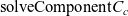

Since dividing the constraint graph into connected components will partition the size variables and constraints into disjoint sets, the time complexity of all executions of solveComponent is $O(\lVert{V}\rVert\lVert{C}\rVert)$
. This is also the time complexity of negative-cycle finding. These two dominate the time complexity of finding the connected components, which is
$O(\lVert{V}\rVert\lVert{C}\rVert)$
. This is also the time complexity of negative-cycle finding. These two dominate the time complexity of finding the connected components, which is $O(\lVert{V}\rVert + \lVert{C}\rVert)$
.
$O(\lVert{V}\rVert + \lVert{C}\rVert)$
.
4.5 Metatheory
In this subsection, we focus on soundness and completeness theorems of various parts of the inference algorithm. The proof sketches and partial proofs for these and for the intermediate lemmas and theorems can be found in Appendix 2.
We first need soundness and completeness of RecCheck. The constraint set returned by RecCheck ensures that variables that should be infinite are constrained to be so, and that variables that shouldn’t be infinite are not. Intuitively, soundness then says that if you have a solution to a constraint set returned by RecCheck, then there must also be a solution to the original constraint set that also ensures the same things. Dually, completeness says that if you have a solution to the original constraint set that ensures these constraints, then it must also be a solution to the constraint set returned by RecCheck.
-1In these theorems, we use the metafunction ${\lfloor{s}\rfloor}$
which returns either the size variable of a finite size expression or
${\lfloor{s}\rfloor}$
which returns either the size variable of a finite size expression or $\infty$
if the given size expression is infinite. Since sizes are (successors of) either a size variable or the infinite size, we have that
$\infty$
if the given size expression is infinite. Since sizes are (successors of) either a size variable or the infinite size, we have that $\lfloor{\hat{\upsilon}^{n}}\rfloor = \upsilon$
and
$\lfloor{\hat{\upsilon}^{n}}\rfloor = \upsilon$
and $\lfloor{\succ{\infty}^n}\rfloor = \infty$
.
$\lfloor{\succ{\infty}^n}\rfloor = \infty$
.
Theorem 4.5
(Soundness of (SRC)) If $\text{RecCheck}(C', \tau, V^*, V^\neq) = C$
, then for every
$\text{RecCheck}(C', \tau, V^*, V^\neq) = C$
, then for every $\rho$
such that
$\rho$
such that $\rho \vDash C$
, given a fresh size variable
$\rho \vDash C$
, given a fresh size variable $\upsilon$
, there exists a
$\upsilon$
, there exists a $\rho'$
such that the following all hold:
$\rho'$
such that the following all hold:
-
1.
$\rho' \vDash C'$
; -
2.
$\rho'\tau = \upsilon$
; -
3.
$\lfloor{\rho' V^*}\rfloor = \upsilon$
; -
4.
$\lfloor{\rho' V^\neq}\rfloor \neq \upsilon$
; -
5. For all
$\upsilon' \in V^\neq$
,
$(\{\upsilon \mapsto \rho\tau\} \circ \rho')(\upsilon') = \rho\upsilon'$
; and -
6. For all
$\tau' \in V^*$
,
$(\{\upsilon \mapsto \rho\tau\} \circ \rho')(\tau') \sqsubseteq \rho\tau'$
.


Theorem 4.6 (Completeness of (CRC))
Suppose the following all hold:
-
$\rho \vDash C'$
;
-
$\rho\tau = \upsilon$
;
-
$\lfloor{\rho V^*}\rfloor = \upsilon$
; and
-
$\lfloor{\rho V^\neq}\rfloor \neq \upsilon$
.


Then $\rho \vDash \text{RecCheck}(C', \tau, V^*, V^\neq)$
.
$\rho \vDash \text{RecCheck}(C', \tau, V^*, V^\neq)$
.
RecCheck returns a constraint set for a single (co)fixpoint definition with a fixed set of position variables; RecCheckLoop, on the other hand, returns a constraint set for an entire mutual (co)fixpoint definition, finding a suitable set of position variables. There are then two properties we want to ensure.
Theorem 4.7 (Correctness of RecCheckLoop)
-
1. RecCheckLoop terminates on all inputs.
-
2. If
$\text{RecCheckLoop}{C', \Gamma, \overline{\tau_k}, \overline{t_k}, \overline{e_k}} = C$
with an initial position variable set
$\mathcal{V}^*$
, then for every
$i \in \overline{k}$
,
$\text{RecCheck}{C', \tau_i, \text{PV}(t_i), \text{SV}(\Gamma, t_i, e_i) \setminus \text{PV}(t_i)} \subseteq C$
with some final position variable set
$\mathcal{V}^*_\subseteq \subseteq \mathcal{V}^*$
.


We also want to ensure that solveComponent and solve actually return solutions of the constraint sets they are solving.
Theorem 4.8 (Correctness of and)
-
1. If the constraint set
$C_c$
contains no negative cycles, then
$\text{solveComponent}{C_c} \vDash C_c$
and -
2.
$\text{solve}{C} \vDash C$
.


Before proceeding onto the main soundness theorems, we need a few lemmas ensuring that the positivity/negativity judgements and algorithmic subtyping are sound and complete with respect to subtyping.
Lemma 4.9
(Soundness of positivity/negativity) Let $\Gamma_{G}, \Gamma$
be environments, t a sized term and
$\Gamma_{G}, \Gamma$
be environments, t a sized term and $\rho_1, \rho_2$
size substitutions. Suppose that
$\rho_1, \rho_2$
size substitutions. Suppose that $\forall \upsilon \in \text{SV}{t}, \rho_1 \upsilon \sqsubseteq \rho_2 \upsilon$
.
$\forall \upsilon \in \text{SV}{t}, \rho_1 \upsilon \sqsubseteq \rho_2 \upsilon$
.
-
1. If
, then
; and -
2. If
, then
.
Lemma 4.10
(Completeness of positivity/negativity) Let $\Gamma_{G}, \Gamma$
be environments, t a sized term and
$\Gamma_{G}, \Gamma$
be environments, t a sized term and $\upsilon \in \text{SV}{t}$
some size variable.
$\upsilon \in \text{SV}{t}$
some size variable.
-
1. If
then
. -
2. If
then
.
Lemma 4.11
(Soundness of algorithmic subtyping) Let $\Gamma_G, \Gamma \vdash t \preceq u \rightsquigarrow C$
, and suppose that
$\Gamma_G, \Gamma \vdash t \preceq u \rightsquigarrow C$
, and suppose that $\rho \vDash C$
. Then
$\rho \vDash C$
. Then $\Gamma_G, \rho \Gamma \vdash \rho t \leq \rho u$
.
$\Gamma_G, \rho \Gamma \vdash \rho t \leq \rho u$
.
Now we are ready to tackle the main theorems, in particular soundness of checking, inference, and well-formedness with respect to the typing rules. We leave completeness of checking and inference as a conjecture, but show that if it holds, then completeness of well-formedness will hold as well.
Theorem 4.12
(Soundness (check/infer)) Let $\Sigma$
be a fixed, well-formed signature,
$\Sigma$
be a fixed, well-formed signature, $\Gamma_G$
a global environment,
$\Gamma_G$
a global environment, $\Gamma$
a local environment, and C a constraint set. Suppose we have the following: [label=)]
$\Gamma$
a local environment, and C a constraint set. Suppose we have the following: [label=)]
-
1.
$\forall \rho \vDash C, {\textrm{WF}({\Gamma_G, \rho \Gamma})}$
. -
2. If
$\exists \Gamma_1, \Gamma_2, e, t$
such that
$\Gamma \equiv \Gamma_1 ({{x} \mathbin{:} {t} \mathbin{:=} {e}}) \Gamma_2$
then
$\forall \upsilon \in \text{SV}(e, t), \upsilon \notin \text{SV}(\Gamma_G, \Gamma_1)$
.


Then the following hold:
-
1. If
, then
$\forall \rho \vDash C \cup C'$
, we have
$\Gamma_G, \rho\Gamma \vdash \rho e : \rho t$
. -
2. If
, then
$\forall \rho \vDash C \cup C'$
, we have
$\Gamma_G, \rho\Gamma \vdash \rho e : \rho t$
.


Conjecture 4.13
(Completeness (check/infer)) Let $\Sigma$
be a fixed, well-formed signature,
$\Sigma$
be a fixed, well-formed signature, $\Gamma_G$
a global environment,
$\Gamma_G$
a global environment, $\Gamma$
a local environment, C a constraint set, and
$\Gamma$
a local environment, C a constraint set, and $\rho \vDash C$
a solution to the constraint set.
$\rho \vDash C$
a solution to the constraint set.
-
1. If
$\Gamma_G, \rho\Gamma \vdash e : \rho t$
, then there exist
$C', \rho', e'$
such that:


• $\rho' \vDash C'$
;
$\rho' \vDash C'$
;
• $\forall \upsilon \in \text{SV}(\Gamma, t), \rho \upsilon = \rho' \upsilon$
; and
$\forall \upsilon \in \text{SV}(\Gamma, t), \rho \upsilon = \rho' \upsilon$
; and
• $C, \Gamma_G, \Gamma \vdash |{e}| \Leftarrow t \rightsquigarrow C', e'$
where
$C, \Gamma_G, \Gamma \vdash |{e}| \Leftarrow t \rightsquigarrow C', e'$
where
 $\Gamma_G, \Gamma \vdash \rho' e'
\approx e$
.
$\Gamma_G, \Gamma \vdash \rho' e'
\approx e$
.
-
2. If
$\Gamma_G, \rho\Gamma \vdash e : t$
, then there exist
$C, \rho', t'$
such that:


• $\rho' \vDash C'$
;
$\rho' \vDash C'$
;
• $\forall \upsilon \in \text{SV}(\Gamma, t), \rho \upsilon = \rho' \upsilon$
; and
$\forall \upsilon \in \text{SV}(\Gamma, t), \rho \upsilon = \rho' \upsilon$
; and
• $C, \Gamma_G, \Gamma \vdash |{e}| \rightsquigarrow C', e' \Rightarrow t'$
where
$C, \Gamma_G, \Gamma \vdash |{e}| \rightsquigarrow C', e' \Rightarrow t'$
where $\Gamma_G, \Gamma \vdash \rho' e' \approx e$
and
$\Gamma_G, \Gamma \vdash \rho' e' \approx e$
and $\Gamma_G, \Gamma \vdash \rho' t \leq t$
.
$\Gamma_G, \Gamma \vdash \rho' t \leq t$
.
Theorem 4.14
(Soundness (well-formedness)) If $\Gamma_G^\circ \rightsquigarrow \Gamma_G$
then
$\Gamma_G^\circ \rightsquigarrow \Gamma_G$
then ${\textrm{WF}({\Gamma_G, \bullet})}$
.
${\textrm{WF}({\Gamma_G, \bullet})}$
.
The completeness theorem for well-formedness is slightly different than expected: a well-formed global environment, when erased, should successfully have sizes inferred. The inferred environment and the original environment also erase to the same bare environment, which can be proven by induction on the size inference derivations.
Theorem 4.15
(Completeness (well-formedness)) If ${\textrm{WF}({\Gamma_G, \bullet})}$
then
${\textrm{WF}({\Gamma_G, \bullet})}$
then $|{\Gamma_G}| \rightsquigarrow \Gamma'_G$
and
$|{\Gamma_G}| \rightsquigarrow \Gamma'_G$
and $|{\Gamma_G}| = |{\Gamma'_G}|$
.
$|{\Gamma_G}| = |{\Gamma'_G}|$
.
5 Prototype Implementation and Evaluation
We have implemented the sized typing algorithm in a beta version of Coq 8.12 (The Coq Development Team and Chan, Reference Chan2021), which can also be found in the supplementary materials. Naturally, the full core language of Coq has more features (irrelevant for sized typing) than CIC $\widehat{\ast}$
, and the implementation has to interact with these as well as other proof assistant features such as elaboration and the vernacular. Furthermore, many details of the sized typing algorithm are left underspecified. In this section, we take a take a brief look at these details, verify the time complexity of the implementation against the theoretical complexities from the previous section, determine its impact on performance as a whole, and discuss the practical feasibility of the implementation as well as the problems encountered.
$\widehat{\ast}$
, and the implementation has to interact with these as well as other proof assistant features such as elaboration and the vernacular. Furthermore, many details of the sized typing algorithm are left underspecified. In this section, we take a take a brief look at these details, verify the time complexity of the implementation against the theoretical complexities from the previous section, determine its impact on performance as a whole, and discuss the practical feasibility of the implementation as well as the problems encountered.
5.1 Architecture of the Coq Kernel
The core type checking/inference algorithm is found in Coq’s kernel. Before reaching the kernel, terms go through a round of pretyping where existential metavariables (essentially typed holes) are solved for, and the recursive indices of fixpoints are determined. Size inference is implemented as an augmentation of the existing type checking/inference algorithm, making use of the recursive indices.
Figure 20 summarizes the relevant file/module structure. Most of the added code specifically for size inference is in the new Sized and Subsizing modules; the remaining structure remains the same as that of Coq 8.12’s codebase (The Coq Development Team, 2021). (Subsizing is only separate from Sized to break circular dependencies: it relies on the global environment, while the environment depends on Sized.)

Figure 20. Selected excerpts of the Coq codebase structure.
The Sized module contains several submodules, four of which are relevant to our performance discussion:
-
State keeps track of the (position) size variables that have been used;
-
SMap defines the data structure for and operations on size substitutions;
-
Constraints defines the data structure for and operations on constraint sets; and
-
RecCheck implements the RecCheck and solve algorithms.
Sized typing is implemented as a vernacular flag that can be set and unset, just like guard checking. By default, the flag is off; the commands
will enable sized typing only. If both are set, then guard checking will only occur if sized typing fails. When sized typing is not set, size annotations are still added, but constraints aren’t collected, meaning that global definitions checked in this state will never be marked as size preserving.
5.2 Analysis of Performance Degradation
When compiling parts of the Coq standard library with sized typing on, we noticed some severe performance degradation. This is bad news if we hope to replace guard checking with sized typing, or even if we simply wish to use sized typing as the primary method of termination or productivity checking throughout. In particular, we examine compilation of the Coq.MSets.MSetList library
Footnote 4
, which is an implementation of finite sets using ordered lists that contains a fair amount of both fixpoints and proof terms and that happens to compile successfully with sized typing on. In this file alone, we find a $5.5\kern-1pt\times$
increase in compilation time with coqc. Other files may have even worse degradation; for an earlier version of the algorithm, there was a
$5.5\kern-1pt\times$
increase in compilation time with coqc. Other files may have even worse degradation; for an earlier version of the algorithm, there was a $15\times$
increase in compilation time for Coq.setoid_ring.Field_theory
Footnote 5
, which is about twice as large as MSetList and contains mostly proofs. We investigate possible causes of the performance degradation and discuss potential solutions.
$15\times$
increase in compilation time for Coq.setoid_ring.Field_theory
Footnote 5
, which is about twice as large as MSetList and contains mostly proofs. We investigate possible causes of the performance degradation and discuss potential solutions.
5.2.1 Profiling Sized Functions
To measure the performance degradation, we compare compiling MSetList against itself with sized typing on and guard checking off, which we refer to as MSetList_sized. Both compilations are run five times each. The compilation times are significantly different ( $t = 463.94$
,
$t = 463.94$
, $p \ll 0.001$
), with MSetList’s compilation time at
$p \ll 0.001$
), with MSetList’s compilation time at $15.122 \pm 0.073$
seconds and MSetList_sized’s at
$15.122 \pm 0.073$
seconds and MSetList_sized’s at $82.660 \pm 0.286$
seconds.
$82.660 \pm 0.286$
seconds.
To identify the source of the slowdown and test our hypothesis that the majority of it is intrinsically due to size inference, we first profile the performance of functions relevant to the Sized module during the compilation. We divide these functions into five groups: the solve and RecCheck functions, the foldmap
Footnote 6 function common to all operations manipulating size annotations on the AST (such as applying size substitutions), the functions in State, the functions in SMap, and the functions in Constraints. Table 2 summarizes the results, as well as the relative time spent in the functions in MSetList_sized. The differences in execution times of the functions in each group are all statistically significant ( $p \ll 0.001$
for all of the t-statistics).
$p \ll 0.001$
for all of the t-statistics).
Table 2. Relevant function runtimes when compiling MSetList vs. MSetList_sized
 $77.2\%$
of the total compilation time in MSetList_sized is taken up by solve and RecCheck. Other Sized-related overhead is smaller, although not insignificant, especially Constraint operations, which form a proportion slightly larger than that of RecCheck. We conjecture that some of this other overhead can be reduced with more clever implementations. For instance, instead of explicitly performing size substitutions, the sizes can be looked up as needed; or instead of explicitly passing around a size state, we could use mutable global state; or constraints could be stored in a data structure incrementally checked for negative cycles, similar to the current implementation of universe level constraints. We therefore focus our attention on solve and RecCheck, where performance degradation may not be limited to mere implementational details.
$77.2\%$
of the total compilation time in MSetList_sized is taken up by solve and RecCheck. Other Sized-related overhead is smaller, although not insignificant, especially Constraint operations, which form a proportion slightly larger than that of RecCheck. We conjecture that some of this other overhead can be reduced with more clever implementations. For instance, instead of explicitly performing size substitutions, the sizes can be looked up as needed; or instead of explicitly passing around a size state, we could use mutable global state; or constraints could be stored in a data structure incrementally checked for negative cycles, similar to the current implementation of universe level constraints. We therefore focus our attention on solve and RecCheck, where performance degradation may not be limited to mere implementational details.
5.2.2 Time Complexity of solve and RecCheck
As shown in Section 4, given a constraint graph from constraint graph C with size variables V, the time complexities of solve and RecCheck are $O(\lVert{V}\rVert\lVert{C}\rVert)$
. Indeed, in Figure 21a, plotting the mean execution times of each of the 155 calls to solve against
$O(\lVert{V}\rVert\lVert{C}\rVert)$
. Indeed, in Figure 21a, plotting the mean execution times of each of the 155 calls to solve against $\lVert{V}\rVert\lVert{C}\rVert$
for that call (shown as blue dots), we see a strong positive correlation (
$\lVert{V}\rVert\lVert{C}\rVert$
for that call (shown as blue dots), we see a strong positive correlation ( $r = 0.983$
). Doing the same for the 186 calls to RecCheck in Figure 21a, we have a weaker positive correlation (
$r = 0.983$
). Doing the same for the 186 calls to RecCheck in Figure 21a, we have a weaker positive correlation ( $r = 0.698$
), likely due to the two visible outliers. (Without the outliers, we have
$r = 0.698$
), likely due to the two visible outliers. (Without the outliers, we have $r = 0.831$
.)
$r = 0.831$
.)

Figure 21. Execution vs. $\lVert{V}\rVert\lVert{C}\rVert$
, residuals,
$\lVert{V}\rVert\lVert{C}\rVert$
, residuals, $\lVert{V}\rVert\lVert{C}\rVert$
distributions for solve and RecCheck.
$\lVert{V}\rVert\lVert{C}\rVert$
distributions for solve and RecCheck.
To verify that the execution times are dominated by linear relationships to $\lVert{V}\rVert\lVert{C}\rVert$
, we fit the data to linear models using least-square regressions (shown as orange lines), and examine the residuals plots in Figure 21c and Figure 21d for solve and RecCheck, respectively. (Note the logarithmic horizontal scale used for clarity, as there are more calls with fewer variables and constraints).
$\lVert{V}\rVert\lVert{C}\rVert$
, we fit the data to linear models using least-square regressions (shown as orange lines), and examine the residuals plots in Figure 21c and Figure 21d for solve and RecCheck, respectively. (Note the logarithmic horizontal scale used for clarity, as there are more calls with fewer variables and constraints).
For solve, the model appears to be a good fit at first, but residuals increase in magnitude as $\lVert{V}\rVert\lVert{C}\rVert$
increases, indicating some additional behaviour unexplained by the model. Similarly, for RecCheck, the model also appears to be a good fit at first, but then follow a downward curving pattern, also indicating additional behaviour unexplained by the model (such as the two outliers).
$\lVert{V}\rVert\lVert{C}\rVert$
increases, indicating some additional behaviour unexplained by the model. Similarly, for RecCheck, the model also appears to be a good fit at first, but then follow a downward curving pattern, also indicating additional behaviour unexplained by the model (such as the two outliers).
Although there might be additional smaller factors influencing the time complexities of solve and RecCheck beyond the number of variables and constraints, we can at least reasonably conclude that execution time increases with $\lVert{V}\rVert\lVert{C}\rVert$
. Since this time complexity is intrinsic to the algorithms and is not due to mere implementational details, and more than three-fourths of the total compilation time is due to solve and RecCheck, the majority of the slowdown is therefore intrinsic and unavoidable.
$\lVert{V}\rVert\lVert{C}\rVert$
. Since this time complexity is intrinsic to the algorithms and is not due to mere implementational details, and more than three-fourths of the total compilation time is due to solve and RecCheck, the majority of the slowdown is therefore intrinsic and unavoidable.
5.2.3 An Explosion of Size Variables
As solve and RecCheck contribute so much to the compilation time and their complexities depend on $\lVert{V}\rVert\lVert{C}\rVert$
, there must be a significant number of calls involving large numbers of variables and constraints. Indeed, Figure 21e and Figure 21f show that despite most calls during compilation of MSetList involving small values of
$\lVert{V}\rVert\lVert{C}\rVert$
, there must be a significant number of calls involving large numbers of variables and constraints. Indeed, Figure 21e and Figure 21f show that despite most calls during compilation of MSetList involving small values of $\lVert{V}\rVert\lVert{C}\rVert$
, the number of calls with large values of
$\lVert{V}\rVert\lVert{C}\rVert$
, the number of calls with large values of $\lVert{V}\rVert\lVert{C}\rVert$
is not trivial.
$\lVert{V}\rVert\lVert{C}\rVert$
is not trivial.
Of course, the presence of large numbers of variables and constraints of only MSetList with sized typing doesn’t tell us whether this is a common property of Coq files on average, but the fact that this occurs in the standard library indicates that it is absolutely possible for an explosion in size variables and constraints to be a significant barrier to the adoption of sized typing for general-purpose use. In fact, this behaviour is easily reproducible with the artificial but comparatively small and simple example in Figure 22. Table 3 lists the number of size variables present in the types and bodies of these definitions, along with the elapsed type checking time reported by Coq.
Table 3. Size variables and time elapsed for definitions in fig:nats


Figure 22. Coq definitions with an explosion in size variables and in elapsed time.
There are two things we can do to reduce the execution time of solve and RecCheck: eliminate constraints when possible, or reduce the number of size variables in definitions. One way to accomplish the first option would be to turn on sized typing only for certain definitions, in particular the ones involving (co)fixpoints where they will be most useful. Then for all other definitions, since no constraints are collected, calls to solve will be trivial regardless of how many size variables they contain.
However, a (co)fixpoint might require that some non-(co)recursive definition with many size variables be size preserving, which means that that definition also needs to be checked with sized typing on, or the (co)fixpoint itself may have a large number of size variables. Furthermore, there’s no clear indication of which definitions might have a large number of size variables and which don’t, leaving it up to a lot of guesswork and experimentation. Using sized typing as a targeted tool for particular programs is not viable if we cannot directly tell which particular programs will benefit the most in terms of tradeoffs between non-structural (co)recursion and performance.
The second option to reduce the number of size variables can be done by allowing manual annotation of (co)inductive types with the infinite size, reducing the number of free size variables that need to be substituted for and that propagate throughout subsequent definitions. For example, the tuple types in Figure 22 can have infinite size annotations without affecting the sizes of the nat arguments. In other words, we allow size annotations in the surface language that users write, which would no longer be plain CIC; as this solution deviates from the philosophy of being wholly backward compatible, it is beyond the scope of this paper.
5.3 Inferring Recursive Indices
As previously mentioned, users aren’t obligated to indicate which fixpoint argument is the one on which we recur, and its position index is inferred during pretyping in the kernel. In Coq, for a mutual fixpoint, this is done by trying the guard predicate on every combination of indices Footnote 7 . This is possible because the guard predicate is a syntactic check, requiring nothing but the elaborated fixpoint term.
Unfortunately, we run into problems when attempting to apply the same strategy to inferring recursive indices through sized typing alone. Because termination checking is inextricably tied to type checking, the entire fixpoint needs to be type checked to verify whether the current set of indices is correct, and this type checking in the kernel can fail if the fixpoint still contains unsolved metavariables. Furthermore, because we only have access to the bare environments (i.e. with no sizes inferred), local definitions in scope at the fixpoint may not yet be known to be size preserving, thus causing the check to fail. As an example, in the following Coq term, id has no size annotations and is therefore treated as not size preserving, even though it ought to be, which causes the recursive call on the smaller argument wrapped in id to not pass type checking.
This suggests that size inference should be done during the pretyping phase: size inference could be viewed as part of the elaboration step from the surface CIC to the core CIC $\widehat{\ast}$
. This, too, is beyond the scope of this paper, especially as there is no past work on formalizing the interaction between size inference and elaboration to build on.
$\widehat{\ast}$
. This, too, is beyond the scope of this paper, especially as there is no past work on formalizing the interaction between size inference and elaboration to build on.
6 Related Work
The history of sized types is vast and varied. Extensive prior accounts are given in dissertations by Frade (Reference Frade2004) and Abel (Reference Abel2006). Here, we focus on two lineages towards sized dependent type theories: first, the more-or-less direct ancestry of CIC $\widehat{\ast}$
, and second, a contrasting line of work on type systems with explicit higher-order sized types.
$\widehat{\ast}$
, and second, a contrasting line of work on type systems with explicit higher-order sized types.
6.1 Ancestry of CIC
$\widehat{\ast}$

Perhaps the most well-known work on sized types is by Hughes et al. (Reference Hughes, Pareto and Sabry1996), who introduce sized types for a Hindley–Milner type system with (co)inductives and a size inference algorithm, as well as the term “sized types”. Their size algebra is more expressive than ours, with size addition $s_1 + s_2$
and constant multiplication
$s_1 + s_2$
and constant multiplication $n \times s$
. Independently, Giméez (Reference Giménez1998) introduces
$n \times s$
. Independently, Giméez (Reference Giménez1998) introduces $\mathfrak{CCR}$
, a Calculus of Constructions (CoC) with guarded types, a type-based termination checking alternative to the earlier syntactic guard condition (Giméez, Reference Giménez1995). There, types are guarded with a type operator
$\mathfrak{CCR}$
, a Calculus of Constructions (CoC) with guarded types, a type-based termination checking alternative to the earlier syntactic guard condition (Giméez, Reference Giménez1995). There, types are guarded with a type operator $\widehat{\cdot}$
, similar to the later modality
$\widehat{\cdot}$
, similar to the later modality $\rhd \cdot$
in modern guarded type theories. Based on a semantic interpretation of
$\rhd \cdot$
in modern guarded type theories. Based on a semantic interpretation of $\mathfrak{CCR}$
, Amadio and Coupet-Grimal (Reference Amadio and Coupet-Grimal1998) introduce a simply-typed lambda calculus (STLC) with coinductives with type labels, corresponding roughly to size annotations with successor sizes.
$\mathfrak{CCR}$
, Amadio and Coupet-Grimal (Reference Amadio and Coupet-Grimal1998) introduce a simply-typed lambda calculus (STLC) with coinductives with type labels, corresponding roughly to size annotations with successor sizes.
Following this, Barthe et al. (Reference Barthe, Frade, Giménez, Pinto and Uustalu2004) and Frade (Reference Frade2004) introduce $\lambda\widehat{~}$
, another STLC with inductives and size annotations with the same size algebra we use, although they are instead called stages. It improves upon the work of Amadio and Coupet-Grimal (Reference Amadio and Coupet-Grimal1998) by adding an implicit form of size polymorphism: the position size variable of fixpoint types are substituted by an arbitrary size expression, just as in Rule fix. Barthe et al. (Reference Barthe, Grégoire and Pastawski2005) extend
$\lambda\widehat{~}$
, another STLC with inductives and size annotations with the same size algebra we use, although they are instead called stages. It improves upon the work of Amadio and Coupet-Grimal (Reference Amadio and Coupet-Grimal1998) by adding an implicit form of size polymorphism: the position size variable of fixpoint types are substituted by an arbitrary size expression, just as in Rule fix. Barthe et al. (Reference Barthe, Grégoire and Pastawski2005) extend $\lambda\widehat{~}$
to System F with F
$\lambda\widehat{~}$
to System F with F $\widehat{~}$
, and introduce and prove correct a size inference algorithm. This includes the RecCheck algorithm that we use. They continue on to extend F
$\widehat{~}$
, and introduce and prove correct a size inference algorithm. This includes the RecCheck algorithm that we use. They continue on to extend F $\widehat{~}$
with sized products (that is, pairs with size annotations) in F
$\widehat{~}$
with sized products (that is, pairs with size annotations) in F $\widehat{_\times}$
(Barthe et al., Reference Barthe, Grégoire and Riba2008), whose size expressions include size addition, and to CIC in CIC
$\widehat{_\times}$
(Barthe et al., Reference Barthe, Grégoire and Riba2008), whose size expressions include size addition, and to CIC in CIC $\widehat{~}$
(Barthe et al., Reference Barthe, Grégoire and Pastawski2006). Our size inference algorithm is based directly on that of CIC
$\widehat{~}$
(Barthe et al., Reference Barthe, Grégoire and Pastawski2006). Our size inference algorithm is based directly on that of CIC $\widehat{~}$
. We add to it global and local definitions and explicitly treat mutually-defined (co)inductives and (co)fixpoints, while removing polarities and subtyping based on these polarities.
$\widehat{~}$
. We add to it global and local definitions and explicitly treat mutually-defined (co)inductives and (co)fixpoints, while removing polarities and subtyping based on these polarities.
However, normalization of CIC $\widehat{~}$
is only a conjecture; it is later proven for the restricted language CIC
$\widehat{~}$
is only a conjecture; it is later proven for the restricted language CIC $\widehat{_-}$
by [Gràoire Sacchini (Reference Grégoire and Sacchini2010) (with only naturals) and by Sacchini (Reference Sacchini2011) (with inductive types). The restrictions include disallowing size variables in the bodies of functions, in the arguments of applications, in the branches of case expressions, and in the indices of inductives; erasing the parameters to constructors; and disallowing strong elimination to types with size variables. We remove these restrictions to allow using sized definitions and for backward compatibility with Coq.
$\widehat{_-}$
by [Gràoire Sacchini (Reference Grégoire and Sacchini2010) (with only naturals) and by Sacchini (Reference Sacchini2011) (with inductive types). The restrictions include disallowing size variables in the bodies of functions, in the arguments of applications, in the branches of case expressions, and in the indices of inductives; erasing the parameters to constructors; and disallowing strong elimination to types with size variables. We remove these restrictions to allow using sized definitions and for backward compatibility with Coq.
Our typing rules and inference algorithm for coinductives and cofixpoints are based on CC $\widehat{\omega}$
(Sacchini, Reference Sacchini2013), which extends CoC with sized coinductive streams. Further extensions to the size algebra are linear sized types in CIC
$\widehat{\omega}$
(Sacchini, Reference Sacchini2013), which extends CoC with sized coinductive streams. Further extensions to the size algebra are linear sized types in CIC $\widehat{_l}$
(Sacchini, Reference Sacchini2014), which adds constant multiplication to a sized CoC with naturals and streams; and well-founded sized types in CIC
$\widehat{_l}$
(Sacchini, Reference Sacchini2014), which adds constant multiplication to a sized CoC with naturals and streams; and well-founded sized types in CIC $\widehat{_\sqsubseteq}$
(Sacchini, Reference Sacchini2015), which changes the premise type checking the (co)fixpoint body in Rules fix and cofix to the recursive reference having any smaller size according to the subsizing rules, rather than the direct predecessor. All three include size inference algorithms similar to that of CIC
$\widehat{_\sqsubseteq}$
(Sacchini, Reference Sacchini2015), which changes the premise type checking the (co)fixpoint body in Rules fix and cofix to the recursive reference having any smaller size according to the subsizing rules, rather than the direct predecessor. All three include size inference algorithms similar to that of CIC $\widehat{~}$
.
$\widehat{~}$
.
There are prototype implementations of CIC $\widehat{_-}$
(Sacchini, Reference Sacchini2015) and CIC
$\widehat{_-}$
(Sacchini, Reference Sacchini2015) and CIC $\widehat{_\sqsubseteq}$
(Sacchini, Reference Sacchini2015). It appears that there were also plans to implement sized types in Coq by Sacchini (Reference Sacchini2016), but seem to be abandoned.
$\widehat{_\sqsubseteq}$
(Sacchini, Reference Sacchini2015). It appears that there were also plans to implement sized types in Coq by Sacchini (Reference Sacchini2016), but seem to be abandoned.
6.2 Past Work in Detail
Past work CIC $\widehat{~}$
, CIC
$\widehat{~}$
, CIC $\widehat{_-}$
, and CC
$\widehat{_-}$
, and CC $\widehat{\omega}$
add sized types to CIC with the explicit philosophy of requiring no size annotations: a user would write bare CIC code, and the type checker would have the simultaneous task of synthesizing and checking types, while also inferring all the size annotations. However, Coq’s core calculus extends quite a bit beyond merely CIC, and the presentation of various analogous features differ subtly but nontrivially. The goal of CIC
$\widehat{\omega}$
add sized types to CIC with the explicit philosophy of requiring no size annotations: a user would write bare CIC code, and the type checker would have the simultaneous task of synthesizing and checking types, while also inferring all the size annotations. However, Coq’s core calculus extends quite a bit beyond merely CIC, and the presentation of various analogous features differ subtly but nontrivially. The goal of CIC $\widehat{\ast}$
is to bring sized types in CIC a few steps closer to Coq, while keeping with the original philosophy. In the process of conforming to Coq’s calculus, to minimize the changes required to it so that a prototype implementation is viable, we must also discard some features from past work.
$\widehat{\ast}$
is to bring sized types in CIC a few steps closer to Coq, while keeping with the original philosophy. In the process of conforming to Coq’s calculus, to minimize the changes required to it so that a prototype implementation is viable, we must also discard some features from past work.
6.2.1 Cumulativity
CIC $\widehat{~}$
and CIC
$\widehat{~}$
and CIC $\widehat{_-}$
are extensions of CIC, with dependent functions, a universe hierarchy, inductive definitions, case expressions, and fixpoints. CC
$\widehat{_-}$
are extensions of CIC, with dependent functions, a universe hierarchy, inductive definitions, case expressions, and fixpoints. CC $\widehat{\omega}$
dually has coinductive streams and cofixpoints instead. CIC
$\widehat{\omega}$
dually has coinductive streams and cofixpoints instead. CIC $\widehat{~}$
and CIC
$\widehat{~}$
and CIC $\widehat{_-}$
differ in that CIC
$\widehat{_-}$
differ in that CIC $\widehat{~}$
includes a size inference algorithm but no proof of strong normalization, while CIC
$\widehat{~}$
includes a size inference algorithm but no proof of strong normalization, while CIC $\widehat{_-}$
is proven to be strongly normalizing, with no size inference algorithm explicitly given. CIC
$\widehat{_-}$
is proven to be strongly normalizing, with no size inference algorithm explicitly given. CIC $\widehat{_-}$
also restricts where size variables may appear in terms. Since CIC
$\widehat{_-}$
also restricts where size variables may appear in terms. Since CIC $\widehat{\ast}$
doesn’t have such restrictions, it can be thought of as an extension of CIC
$\widehat{\ast}$
doesn’t have such restrictions, it can be thought of as an extension of CIC $\widehat{~}$
combined with CC
$\widehat{~}$
combined with CC $\widehat{\omega}$
, featuring sized (mutual) (co)inductive types and (mutual) (co)fixpoints, and further adding universe cumulativity, which is an existing feature in Coq. As noted in Section 3, cumulativity and impredicativity complicate the set-theoretic model by Sacchini (Reference Sacchini2011).
$\widehat{\omega}$
, featuring sized (mutual) (co)inductive types and (mutual) (co)fixpoints, and further adding universe cumulativity, which is an existing feature in Coq. As noted in Section 3, cumulativity and impredicativity complicate the set-theoretic model by Sacchini (Reference Sacchini2011).
6.2.2 Definitions
Coq’s core calculus contains two kinds of variables:
Footnote 8
one for local bindings from functions, function types, and let expressions, and one for global bindings from vernacular declarations such as ${\mathtt{{{Definition}}}}$
and
${\mathtt{{{Definition}}}}$
and ${\mathtt{{{Axiom}}}}$
(which we call constants). CIC
${\mathtt{{{Axiom}}}}$
(which we call constants). CIC $\widehat{\ast}$
adds let expressions and global declarations to CIC
$\widehat{\ast}$
adds let expressions and global declarations to CIC $\widehat{~}$
, with separate local and global environments, and definitions in the environments in the style of a PTS with definitions (Severi and Poll, Reference Severi and Poll1993).
$\widehat{~}$
, with separate local and global environments, and definitions in the environments in the style of a PTS with definitions (Severi and Poll, Reference Severi and Poll1993).
Global definitions and let expressions let us define aliases for types for concision and organization of code, which necessitates a form of size polymorphism if we want the aliases to behave as we expect. For instance, if we globally define
![]() , and later want to define an addition function with type
, and later want to define an addition function with type $N \rightarrow N \rightarrow N$
, it would not be correct to perform the naïve substitution to get
$N \rightarrow N \rightarrow N$
, it would not be correct to perform the naïve substitution to get
![]() : addition intuitively does not always return something of the same size.
: addition intuitively does not always return something of the same size.
What we want instead is to allow a different size for each use of N, so that the above type reduces to
![]() . This means N must be polymorphic in the sizes involved in its definition, the same kind of rank-1 or prenex polymorphism in ML-style let polymorphism for type variables. To retain backward compatibility, there is no explicit size quantification or application — every definition and let binding is implicitly quantified over all size variables involved. The corresponding notion of size instantiation comes in the form of size substitution annotations on variables and constants, so that
. This means N must be polymorphic in the sizes involved in its definition, the same kind of rank-1 or prenex polymorphism in ML-style let polymorphism for type variables. To retain backward compatibility, there is no explicit size quantification or application — every definition and let binding is implicitly quantified over all size variables involved. The corresponding notion of size instantiation comes in the form of size substitution annotations on variables and constants, so that $N^{\{\upsilon \mapsto s\}}$
for instance reduces to
$N^{\{\upsilon \mapsto s\}}$
for instance reduces to
![]() .
.
Having definitions and annotated variables and constants also means we need to now allow sizes to appear not only in the bodies of let expressions but also in the bodies of functions and in the branches of case expressions, in contrast to the restrictions of CIC $\widehat{_-}$
.
$\widehat{_-}$
.
6.2.3 Polarities
(co)inductive definitions in CIC $\widehat{_-}$
are also annotated with polarities for each of its parameters to augment the subtyping relation. For example, if the type parameter of the usual
$\widehat{_-}$
are also annotated with polarities for each of its parameters to augment the subtyping relation. For example, if the type parameter of the usual ![]() type is given a positive polarity, then
type is given a positive polarity, then
![]() holds because
holds because
![]() holds, which in turn holds because
holds, which in turn holds because $\hat{s}$
is a larger size than s. Similarly, a negative polarity reverses the subtyping relation, while an invariant polarity induces no subtyping relation from the parameters at all. It is not known whether these polarity annotations are inferrable from the (co)inductive definitions alone, so again in the name of backward compatibility, CIC
$\hat{s}$
is a larger size than s. Similarly, a negative polarity reverses the subtyping relation, while an invariant polarity induces no subtyping relation from the parameters at all. It is not known whether these polarity annotations are inferrable from the (co)inductive definitions alone, so again in the name of backward compatibility, CIC $\widehat{\ast}$
doesn’t have these annotations, and treats all parameters as invariant. This aligns with Coq’s current behaviour, where list
$\widehat{\ast}$
doesn’t have these annotations, and treats all parameters as invariant. This aligns with Coq’s current behaviour, where list
![]() is not a subtype of list
is not a subtype of list
![]() despite the presence of cumulativity where
despite the presence of cumulativity where
![]() is a subtype of
is a subtype of
![]() .
.
Unfortunately, the invariance of parameters and subtyping of sized (co)inductive types interferes with nested (co)inductive types, where the type itself may appear as a parameter to another type in the type of its constructors. Subject reduction is violated: it becomes possible to have a well-typed term that becomes no longer well typed after a reduction step, as demonstrated in in Subsection 3.2. The approach CIC $\widehat{\ast}$
takes is to disallow nested (co)inductives, removing them from CIC
$\widehat{\ast}$
takes is to disallow nested (co)inductives, removing them from CIC $\widehat{~}$
.
$\widehat{~}$
.
6.2.4 Implementation
Whereas CIC $\widehat{\ast}$
can be seen as an extension of CIC
$\widehat{\ast}$
can be seen as an extension of CIC $\widehat{~}$
and CC
$\widehat{~}$
and CC $\widehat{\omega}$
, its implementation is an extension of Coq: all features of Coq orthogonal to sized types remain untouched, such as universe polymorphism, strict
$\widehat{\omega}$
, its implementation is an extension of Coq: all features of Coq orthogonal to sized types remain untouched, such as universe polymorphism, strict ![]() , various primitives, modules, and so on. The implementation also retains Coq’s nested (co)inductives, especially as it doesn’t appear possible for size inference to produce the kind of annotations that break subject reduction.
, various primitives, modules, and so on. The implementation also retains Coq’s nested (co)inductives, especially as it doesn’t appear possible for size inference to produce the kind of annotations that break subject reduction.
6.3 Higher-Order Sized Types
For the purposes of size inferrability from unannotated code, the type systems from $\lambda\widehat{~}$
up to CIC
$\lambda\widehat{~}$
up to CIC $\widehat{~}$
and its variations treat sizes as merely annotations and feature only what can be considered as prenex size polymorphism. On the other hand, Abel (Reference Abel2006) introduces F
$\widehat{~}$
and its variations treat sizes as merely annotations and feature only what can be considered as prenex size polymorphism. On the other hand, Abel (Reference Abel2006) introduces F $\widehat{_\omega}$
, a sized type system for System F
$\widehat{_\omega}$
, a sized type system for System F $_\omega$
that treats size as a kind, which therefore allows for higher-order size polymorphism via explicit quantification. While F
$_\omega$
that treats size as a kind, which therefore allows for higher-order size polymorphism via explicit quantification. While F $\widehat{_\omega}$
subsumes F
$\widehat{_\omega}$
subsumes F $\widehat{~}$
and uses the same size algebra, it uses recursive and corecursive type constructors (
$\widehat{~}$
and uses the same size algebra, it uses recursive and corecursive type constructors ( $\mu$
- and
$\mu$
- and $\nu$
-types) rather than inductive (and coinductive) type definitions.
$\nu$
-types) rather than inductive (and coinductive) type definitions.
Higher-order sized types of the same flavour are implemented in a dependently-typed setting in MiniAgda (Abel, 2010). To avoid inconsistencies introduced by the interplay between sized types and pattern matching, it also introduces bounded size patterns $\upsilon_1 < \upsilon_2$
. Abel (Reference Abel2012) expands upon the theoretical side with bounded size quantification
$\upsilon_1 < \upsilon_2$
. Abel (Reference Abel2012) expands upon the theoretical side with bounded size quantification $\forall \upsilon \mathrel{<} s\mathpunct{.} t$
and well-founded recursion on sizes, which are also implemented in MiniAgda. Abel and Pientka (Reference Abel and Pientka2016) combine well-founded sized types and copatterns for System F
$\forall \upsilon \mathrel{<} s\mathpunct{.} t$
and well-founded recursion on sizes, which are also implemented in MiniAgda. Abel and Pientka (Reference Abel and Pientka2016) combine well-founded sized types and copatterns for System F $_\omega$
with (co)recursive type constructors in F
$_\omega$
with (co)recursive type constructors in F $_\omega^{\text{cop}}$
(which was cited as the inspiration for CIC
$_\omega^{\text{cop}}$
(which was cited as the inspiration for CIC $\widehat{_\sqsubseteq}$
).
$\widehat{_\sqsubseteq}$
).
Abel et al. (Reference Abel, Vezzosi and Winterhalter2017) prove normalization of a higher-order sized dependent type theory with naturals, but without bounded size quantification. To our knowledge, this is the only formalization of higher-order sized dependent types in the literature. Additionally, they also add a notion of size irrelevance so that more terms are convertible when their sizes don’t matter; this is an orthogonal feature that can be added to CIC $\widehat{\ast}$
as well, since the issues size irrelevance aims to resolve can also arise here.
$\widehat{\ast}$
as well, since the issues size irrelevance aims to resolve can also arise here.
Sized types with higher-order bounded size quantification are implemented in Agda
Footnote 9
; however, it is known to be inconsistent
Footnote 10
. In short, it is possible to express the well-foundedness of sizes within Agda, but the infinite size $\infty$
itself is not well founded, as
$\infty$
itself is not well founded, as $\infty + 1 = \infty$
and
$\infty + 1 = \infty$
and $\infty < \infty$
hold, making it possible to derive a contradiction.
$\infty < \infty$
hold, making it possible to derive a contradiction.
7 Perspectives and the Future of Sized Types
We have introduced CIC $\widehat{\ast}$
, a sized type system based on CIC and made to be compatible with Coq, more than a decade since (prenex, fully-inferrable) sized types for CIC were first introduced in CIC
$\widehat{\ast}$
, a sized type system based on CIC and made to be compatible with Coq, more than a decade since (prenex, fully-inferrable) sized types for CIC were first introduced in CIC $\widehat{~}$
and CIC
$\widehat{~}$
and CIC $\widehat{_-}$
. And yet, despite good metatheoretical properties having been established for CIC
$\widehat{_-}$
. And yet, despite good metatheoretical properties having been established for CIC $\widehat{_-}$
, no functioning attempt at implementing sized types in Coq has previously been made. This we have done, finding significant performance problems caused by size inference for definitions yielding an explosion in size variables.
$\widehat{_-}$
, no functioning attempt at implementing sized types in Coq has previously been made. This we have done, finding significant performance problems caused by size inference for definitions yielding an explosion in size variables.
This doesn’t necessarily spell doom for CIC $\widehat{\ast}$
. The seasoned type system implementor may employ implementational tricks to improve performance in practice. Perhaps with some program analysis of how definitions are used, certain size variables known to be irrelevant could immediately be instantiated to the infinite size; maybe a dependency analysis would reveal which definitions need to be checked with the sized typing flag turned on. Our naïve implementation tries to be as general as possible to accept as many programs as possible, and heuristics could be used to guess where and why the user wants to use sized types, whittling down the number of open possibilities for size-inferred programs.
$\widehat{\ast}$
. The seasoned type system implementor may employ implementational tricks to improve performance in practice. Perhaps with some program analysis of how definitions are used, certain size variables known to be irrelevant could immediately be instantiated to the infinite size; maybe a dependency analysis would reveal which definitions need to be checked with the sized typing flag turned on. Our naïve implementation tries to be as general as possible to accept as many programs as possible, and heuristics could be used to guess where and why the user wants to use sized types, whittling down the number of open possibilities for size-inferred programs.
But all of these feel like arbitrary and potentially fragile hacks—and perhaps it’s because they are. We have discussed some more sensible solutions to not only the performance problems but also the theoretical ones: Why don’t we explicitly quantify over the size variables of a definition to specify which ones are actually relevant? Why don’t we require that all recursive arguments be marked? Why not solve the problem of nested inductives using polarities? but we immediately shoot them down because they require additional work from the user’s perspective and therefore violate the philosophy of backward compatibility. Perhaps this philosophy maintained for more than a decade of past work from $\lambda\widehat{~}$
to CIC
$\lambda\widehat{~}$
to CIC $\widehat{_\sqsubseteq}$
is wrong.
$\widehat{_\sqsubseteq}$
is wrong.
So far, size inference seems to work for programs because the notion of programs were merely single terms. Inference was merely extracting hidden information already present in the term. The moment we introduce a little modularity with definitions, we don’t have concrete information on how these definitions will be used, and by being as general as possible to accommodate all usages, we end up with terrible performance. Inference becomes a guessing game we are losing.
If we make size quantification, abstraction, and application explicit, then there won’t be any more size variables involved than are strictly necessary. To ease the tedious burden of all the extra annotations from the user, sizes that can be deduced could be marked as implicit and filled in by the elaborator, as is done for terms. The performance would likely still be better than full inference due to the smaller number of size variables, and because it would be reasonable to expect the elaborator to also fail due to a lack of information rather than only on ill-typed terms. Another benefit of explicit sized types is that it can easily be extended to higher-order size quantification. This appears to be the best future direction for sized types; after all, Agda, which uses explicit sizes, is still to date the only practical proof assistant with sized types.
So is sized typing for Coq practical? Our answer is that it might be—but only if we allow ourselves to ask users to put in a little work as well.
Acknowledgements
We gratefully thank Bruno Barras, Amin Timany, and Andreas Abel for helpful discussions on the metatheory, in particular on strong normalization, and Felipe Bañados Schwerter for testing the implementation and finding bugs, as well as the anonymous reviewers for their time and patience in providing helpful comments.
We acknowledge the support of the Natural Sciences and Engineering Research Council of Canada (NSERC), funding reference number RGPIN-2019-04207, and the Canada Graduate Scholarships – Master’s (CGS M) programme. Cette recherche a été financée par le Conseil de recherches en sciences naturelles et en génie du Canada (CRSNG), numéro de référence RGPIN-2019-04207, et le Programme de bourses d’études supérieures du Canada au niveau de la maitrise (BESC M).
9 Conflicts of Interest.
None.
Well-Formedness of (Co)Inductive Definitions
In this section we define what it means for a (co)inductive definition to be well-formed, including some required auxillary definitions. A signature is then well formed if each of its (co)inductive definitions are well-formed. Note that although we prove subject reduction for CIC $\widehat{\ast}$
without nested inductive types, we include their definitions for completeness.
$\widehat{\ast}$
without nested inductive types, we include their definitions for completeness.
Definition 1.1
(Strict Positivity) Given some existing signature $\Sigma$
, the variable x occurs strictly positively in the term t, written
$\Sigma$
, the variable x occurs strictly positively in the term t, written $x {\mathrel{\oplus}} t$
, if any of the following holds:
$x {\mathrel{\oplus}} t$
, if any of the following holds:
-
$x \notin \text{FV}(t)$
-
$t \mathrel{\approx} x ~ \overline{e}$
and
$x \notin \text{FV}(\overline{e})$
-
$t \mathrel{\approx} \prod{x}{u}{v}$
and
$x \notin \text{FV}(u)$
and
$x \mathrel{\oplus} v$


If nested (co)inductive types are permitted, then $x \mathrel{\oplus} t$
may hold if the following also holds:
$x \mathrel{\oplus} t$
may hold if the following also holds:
-
$t \mathrel{\approx} I_k^\infty ~ \overline{p} ~ \overline{a}$
where
${{\langle{I_i}{\Delta_p}} \mathbin{:} \_ \rangle \mathbin{:=} \langle
{c_j}: \Pi {\Delta_j} \mathpunct{.} {I_j} \text{dom}(\Delta_p)\overline{t}_j\rangle
}\in \Sigma$
for some
$k \in \overline{\imath}$
and all of the following hold:


• $\lVert{\overline{p}}\rVert = \lVert{\Delta_p}\rVert$
• $x \notin \text{FV}(\overline{a})$
• For every j, if $I_j = I_k$
, then
$I_j = I_k$
, then
![]()
Definition 1.2
(Nested Positivity) Given some existing signature $\Sigma$
, the variable x is nested positive in t of
$\Sigma$
, the variable x is nested positive in t of $I_k$
, written
$I_k$
, written
![]() , if
, if $\langle I_i \Delta_p :\_ \rangle\mathbin{:=} \_ \in \Sigma$
for some
$\langle I_i \Delta_p :\_ \rangle\mathbin{:=} \_ \in \Sigma$
for some $k \in \overline{\imath}$
and any of the following holds:
$k \in \overline{\imath}$
and any of the following holds:
-
$t \mathrel{\approx} {I_k^\infty}{\overline{p}}{\overline{a}}$
and
$\lVert{\overline{p}}\rVert = \lVert{\Delta_p}\rVert$
and
$x \notin \text{FV}(\overline{a})$
-
$t \mathrel{\approx} \prod{x}{u}{v}$
and
$x \mathrel{\oplus} u$
and


In short,
![]() if
if
 $t \mathrel{\approx}
{\Pi {\Delta} \mathpunct{.} {I}\overline{p}\overline{a}}$
and
$t \mathrel{\approx}
{\Pi {\Delta} \mathpunct{.} {I}\overline{p}\overline{a}}$
and $x \mathrel{\oplus} \Delta$
and
$x \mathrel{\oplus} \Delta$
and $x \notin \text{FV}(\overline{a})$
.
$x \notin \text{FV}(\overline{a})$
.
Note that if nested (co)inductive types are permitted, then strict and nested positivity are mutually defined.
Definition 1.3 (Constructor Type) The term t is a constructor type for I when:
-
$t = I ~ \overline{e}$
; or
-
$t = \prod{x}{u}{v}$
where
$x \notin \text{FV}{u}$
and v is a constructor type for I; or
-
$t = u \to v$
where
$x \mathrel{\oplus} u$
and v is a constructor type for I.


Note that in particular, this means that $t = \Pi \Delta \mathpunct{.} I ~ \overline{e}$
such that
$t = \Pi \Delta \mathpunct{.} I ~ \overline{e}$
such that $I \mathrel{\oplus} u$
for every
$I \mathrel{\oplus} u$
for every $u \in {codom}{\Delta}$
, and the recursive arguments of t are not dependent.
$u \in {codom}{\Delta}$
, and the recursive arguments of t are not dependent.
Definition 1.4
(Well-formedness of (co)inductiveDefinitions) Suppose we have some signature $\Sigma$
and some global environment
$\Sigma$
and some global environment $\Gamma_G$
. Consider the following (co)inductive definition, where
$\Gamma_G$
. Consider the following (co)inductive definition, where $\overline{p} = {dom}{\Delta_p}$
.
$\overline{p} = {dom}{\Delta_p}$
.
 \begin{align*}
\langle I_i\Delta_p \mathbin{:} \Pi {\Delta_i}\mathpunct{.} U_i\rangle \mathbin{:=}
\langle c_j \Pi\Delta_j. I_j \overline{p}\overline{t}_j\rangle
\end{align*}
\begin{align*}
\langle I_i\Delta_p \mathbin{:} \Pi {\Delta_i}\mathpunct{.} U_i\rangle \mathbin{:=}
\langle c_j \Pi\Delta_j. I_j \overline{p}\overline{t}_j\rangle
\end{align*}
This (co)inductive definition is well-formed if the following all hold:
1. For every i, there is some
$U'_i$
such that
$\Sigma, \Gamma_G, \Delta_p \vdash {\Pi {\Delta_i} \mathpunct{.} {U_i}} : U'_i$
holds.2. For every j, there is some
$U_j$
such that
$\Sigma, \Gamma_G, \Delta_p(I_j^\infty:
\Pi\Delta_p\mathpunct{.} \Pi \Delta_i \mathpunct{.} U_i) \vdash
\Pi\Delta_j\mathpunct{.} I_j^\infty ~ \overline{p} ~ \overline{t}_j : U_j$
holds.3. For every j,
$\Pi\Delta_j\mathpunct{.} I_j\overline{p}\overline{t}_j$
is a constructor type for
$I_j$
. Note that this implies
$I_j \mathrel{\oplus} {codom}{\Delta_j}$
.4. For every i, j, all (co)inductive types in the terms
${codom}{\Delta_p}, {codom}{\Delta_i}, {codom}{\Delta_j}$
are annotated with
$\infty$
.


Well-formedness of a signature $\Sigma$
is then defined in terms of the well-formedness of its (co)inductive definitions, given below.
$\Sigma$
is then defined in terms of the well-formedness of its (co)inductive definitions, given below.
Inference Soundness and Completeness Proofs
Here we provide some more detailed proof sketches for the various soundness and completeness theorems found in Subsection 4.5. Further details when not specified can be found in Barthe et al. (2005), Barthe et al. (2006), and Sacchini (2013).
Theorem 2.1
(Soundness of (SRC)) If $\text{RecCheck}(C', \tau, V^*, V^\neq) = C$
, then for every
$\text{RecCheck}(C', \tau, V^*, V^\neq) = C$
, then for every $\rho$
such that
$\rho$
such that $\rho \vDash C$
, given a fresh size variable
$\rho \vDash C$
, given a fresh size variable $\upsilon$
, there exists a
$\upsilon$
, there exists a $\rho'$
such that the following all hold:
$\rho'$
such that the following all hold:
1.
$\rho' \vDash C'$
;2.
$\rho'\tau = \upsilon$
;3.
$\lfloor{\rho' V^*}\rfloor = \upsilon$
;4.
$\lfloor{\rho' V^\neq}\rfloor \neq \upsilon$
;5. For all
$\upsilon' \in V^\neq$
,
$(\{\upsilon \mapsto \rho\tau\} \circ \rho')(\upsilon') = \rho\upsilon'$
; and6. For all
$\tau' \in V^*$
,
$(\{\upsilon \mapsto \rho\tau\} \circ \rho')(\tau') \sqsubseteq \rho\tau'$
.


[Partial]. Let $C^\iota$
be C with all vertices in
$C^\iota$
be C with all vertices in
![]() removed. By the definition of RecCheck, since all negative cycles in C’ are removed and the only constraints that are added are of the form
removed. By the definition of RecCheck, since all negative cycles in C’ are removed and the only constraints that are added are of the form $\infty \sqsubseteq s$
,
$\infty \sqsubseteq s$
, $C^\iota$
has no negative cycles either. Let
$C^\iota$
has no negative cycles either. Let
![]() . Note that the constraints
. Note that the constraints $\tau \sqsubseteq V^\iota$
are in
$\tau \sqsubseteq V^\iota$
are in $C^\iota$
. Then we are able to compute the weights
$C^\iota$
. Then we are able to compute the weights $w_i$
of the shortest paths from
$w_i$
of the shortest paths from $\tau$
to
$\tau$
to $\bigsqcup V^\iota$
with respect to
$\bigsqcup V^\iota$
with respect to $C^\iota$
. According to Barthe et al. (2005), these weights are nonnegative. Then we can define
$C^\iota$
. According to Barthe et al. (2005), these weights are nonnegative. Then we can define $\rho' := \rho \circ \{\upsilon_i \mapsto \hat{\upsilon}^{w_i} \mid \upsilon_i \in \bigsqcup V^\iota, \rho\upsilon_i \neq \infty\}$
.
$\rho' := \rho \circ \{\upsilon_i \mapsto \hat{\upsilon}^{w_i} \mid \upsilon_i \in \bigsqcup V^\iota, \rho\upsilon_i \neq \infty\}$
.
1. The proof is more involved; see Barthe et al. (2005).
2. The shortest path from
$\tau$
to itself is no path at all, so
$\rho'\tau = \upsilon$
.3. Since
$V^* \subseteq V^\iota \subseteq \bigsqcup V^\iota$
, for every
$\upsilon_i \in V^*$
,
$\rho'\upsilon_i = \hat{\upsilon}^{w_i}$
where
$w_i$
is the weight of the shortest path from
$\upsilon$
to
$\upsilon_i$
, and its size variable is obviously
$\upsilon$
.4. Let
$\upsilon' \in V^\neq$
. If
$\upsilon' \in \bigsqcup V^\iota$
, then
$\infty \sqsubseteq \upsilon'$
must be in C, and therefore
$\rho\upsilon' = \infty$
, so
$\rho'\upsilon' = \rho\upsilon'$
. Otherwise, if
$\upsilon' \notin \bigsqcup V^\iota$
, we again have
$\rho'\upsilon' = \rho\upsilon'$
. Since
$\upsilon$
is fresh, it could not be mapped to by
$\rho$
, so the size variable of
$\rho\upsilon'$
cannot be
$\upsilon$
.5. Let
$\upsilon' \in V^\neq$
. If
$\upsilon' \in \bigsqcup V^\iota$
, then we must have the constraint
$\infty \sqsubseteq \upsilon'$
in C, so
$\rho\upsilon' = \infty$
. Therefore,
$(\{\upsilon \mapsto \rho\tau\} \circ \rho')\upsilon' = (\{\upsilon \mapsto \rho\tau\} \circ \rho)\upsilon' = \rho\upsilon'$
.6. Let
$\tau' \in V^*$
. Note that
$V^* \subseteq V^\iota \subseteq \bigsqcup V^\iota$
. Then letting w’ be the weight of the shortest path from
$\upsilon$
to
$\tau'$
, we have
$\rho'\tau' = \hat{\upsilon}^{w'}$
, and
$(\{\upsilon \mapsto \rho\tau\} \circ \rho')\tau' = \succ{\rho\tau}^{w'}\!$
. Since
$\rho \vDash C$
and there is a path of weight w’ from
$\tau$
to
$\tau'$
in C, we have
$\succ{\rho\tau}^{w'}\! \sqsubseteq \rho\tau'$
.


Theorem 2.2 (Completeness of (CRC))
Suppose the following all hold:
-
$\rho \vDash C'$
;
-
$\rho\tau = \upsilon$
;
-
$\lfloor{\rho V^*}\rfloor = \upsilon$
; and
-
$\lfloor{\rho V^\neq}\rfloor \neq \upsilon$
.


Then $\rho \vDash \text{RecCheck}(C', \tau, V^*, V^\neq)$
.
$\rho \vDash \text{RecCheck}(C', \tau, V^*, V^\neq)$
.
Proof. Let $C = \text{RecCheck}(C', \tau, V^*, V^\neq)$
. To show that
$C = \text{RecCheck}(C', \tau, V^*, V^\neq)$
. To show that $\rho \vDash C$
, we need to show that for every constraint
$\rho \vDash C$
, we need to show that for every constraint $s_1 \sqsubseteq s_2$
in C,
$s_1 \sqsubseteq s_2$
in C, $\rho s_1 \sqsubseteq \rho s_2$
holds. Since
$\rho s_1 \sqsubseteq \rho s_2$
holds. Since $\rho \vDash C'$
, this means we need to show that
$\rho \vDash C'$
, this means we need to show that $\rho$
satisfies every constraint added to C’ in RecCheck. We handle them step by step. Let
$\rho$
satisfies every constraint added to C’ in RecCheck. We handle them step by step. Let
![]() , and let
, and let $V^-$
be the set of size variables involved in some negative cycle in C’.
$V^-$
be the set of size variables involved in some negative cycle in C’.
Step 1:
$\tau \sqsubseteq V^\iota$
. Since we have
$\rho \tau = \upsilon$
and
$\rho V^* = \hat{\upsilon}^{n}$
for some n by assumption,
$\rho \tau \sqsubseteq \rho V^\iota$
holds.Step 2:
$\infty \sqsubseteq V^-$
. For all size variables
$\upsilon' \in V^-$
, since being in a negative cycle transitively implies a subsizing relation
$\hat{\upsilon}'^{n} \sqsubseteq \upsilon'$
for some n, the only way for
$\rho \hat{\upsilon}'^{n} \sqsubseteq \rho \upsilon'$
to hold is if
$\rho \upsilon' = \infty$
, which satisfies
$\infty \sqsubseteq \rho \upsilon'$
.Step 4:
$\infty \sqsubseteq (\bigsqcup V^\neq \cap \bigsqcup V^\iota)$
. Since
$\rho V^\neq$
and
$\rho V^\iota$
have different size variables by assumption, if a size variable
$\upsilon'$
is in both
$\bigsqcup V^\neq$
and
$\bigsqcup V^\iota$
, it must be set to
$\infty$
, which satisfies
$\infty \sqsubseteq \upsilon'$
.


Theorem 2.3 (Correctness of RecCheckLoop)
1. RecCheckLoop terminates on all inputs.
2. If
$\text{RecCheckLoop}{C', \Gamma, \overline{\tau_k}, \overline{t_k}, \overline{e_k}} = C$
with an initial position variable set
$\mathcal{V}^*$
, then for every
$i \in \overline{k}$
,
$\text{RecCheck}{C', \tau_i, \text{PV}(t_i), \text{SV}(\Gamma, t_i, e_i) \setminus \text{PV}(t_i)} \subseteq C$
with some final position variable set
$\mathcal{V}^*_\subseteq \subseteq \mathcal{V}^*$
.


Proof [Sketch].
1. RecCheckLoop does a recursive call only when RecCheck fails with a size variable set V, which by definition is a subset of
$\text{PV}(t_i)$
for some
$t_i$
. Since V is removed from
$\mathcal{V}^*$
every time,
$\text{PV}(\overline{t_k})$
is the decreasing measure of RecCheckLoop.2. Again,
$\mathcal{V}^*$
is only removed from, not added to, so the final set must be a subset of the initial set. By inspection, C is a union of the constraints returned by RecCheck when they all succeed.


Theorem 2.4 (Correctness of and)
1. If the constraint set
$C_c$
contains no negative cycles, then
$\text{solveComponent}{C_c} \vDash C_c$
and2.
$\text{solve}{C} \vDash C$
.


Proof [Sketch].
1. By Cormen et al. (2009), any constant shift (
$w_{\max}$
, in our case) of a shortest-path solution is a valid solution to the difference constraint problem.2. By the same reasoning for RecCheck, any variables involved in negative cycles must be set to
$\infty$
in a solution. Remaining constraints are solved by solveComponent.


Before proceeding, we need a few lemmas ensuring that the positivity/negativity judgements and algorithmic subtyping are sound and complete with respect to subtyping.
Lemma 2.5
(Soundness of positivity/negativity) Suppose that $\forall \upsilon \in \text{SV}{t}, \rho_1 \upsilon \sqsubseteq \rho_2 \upsilon$
.
$\forall \upsilon \in \text{SV}{t}, \rho_1 \upsilon \sqsubseteq \rho_2 \upsilon$
.
1. If
$\gg \vdash \upsilon \text{pos} t$
, then
$\gg \vdash \rho_1 t \leq \rho_2 t$
; and2. If
$\gg \vdash \upsilon \neg t$
, then
$\gg \vdash \rho_2 t \leq \rho_1 t$
.


Proof [Sketch]. By mutual induction on the positivity and negativity rules in Figure 7.
Lemma 2.6 (Completeness of positivity/negativity)
1. If
$\Gamma_G, \Gamma \vdash t \leq
t [\upsilon := {\hat{\upsilon}}]
$
then
$\gg \vdash \upsilon \text{pos} t$
.2. If
$\Gamma_G, \Gamma \vdash
t [\upsilon := \hat{\upsilon}]
\leq t$
then
$\gg \vdash \upsilon \neg t$
.


Proof [Sketch]. By induction on the subtyping rules in Figure 6.
Lemma 2.7
(Soundness of algorithmic subtyping) Let $\Gamma_G, \Gamma \vdash t \preceq u \rightsquigarrow C$
, and suppose that
$\Gamma_G, \Gamma \vdash t \preceq u \rightsquigarrow C$
, and suppose that $\rho \vDash C$
. Then
$\rho \vDash C$
. Then $\Gamma_G, \rho \Gamma \vdash \rho t \leq \rho u$
.
$\Gamma_G, \rho \Gamma \vdash \rho t \leq \rho u$
.
Proof [Sketch]. By induction on the algorithmic subtyping rules in Figure 14.
The following lemma and corollary asserting the absence of certain size variables will later let us commute some substitutions.
Lemma 2.8.
1. If
$\Gamma_G, \Gamma \vdash e^\circ \Leftarrow t \rightsquigarrow C, e$
, then
$\forall \upsilon \in \text{SV}{e}, \upsilon \notin \text{SV}{\Gamma_G, \Gamma}$
.2. If
$\Gamma_G, \Gamma \vdash e^\circ \rightsquigarrow C, e \Rightarrow t$
, then
$\forall \upsilon \in \text{SV}{e}, \upsilon \notin \text{SV}{\Gamma_G, \Gamma}$
.


Proof [Sketch]. By mutual induction on the checking and inference rules of the algorithm. For checking, it follows by the induction hypothesis on the inference premise. For inference, most cases are straightforward applications of the induction hypothesis; new size annotations are only introduced in e in Rules a-ind and a-ind-star, which introduce fresh size variables that are by definition not in $\text{SV}{\Gamma_G, \Gamma}$
.
$\text{SV}{\Gamma_G, \Gamma}$
.
Corollary 11.9
If $\Gamma^\circ_G D^\circ \rightsquigarrow \Gamma_G D$
for bare and sized declarations
$\Gamma^\circ_G D^\circ \rightsquigarrow \Gamma_G D$
for bare and sized declarations $D^\circ, D$
, then
$D^\circ, D$
, then $\forall \upsilon \in \text{SV}(D), \upsilon \notin \Gamma_G$
.
$\forall \upsilon \in \text{SV}(D), \upsilon \notin \Gamma_G$
.
Finally, we can proceed with the main theorems.
Theorem 2.10
(Soundness (check/infer)) Let $\Sigma$
be a fixed, well-formed signature,
$\Sigma$
be a fixed, well-formed signature, $\Gamma_G$
a global environment,
$\Gamma_G$
a global environment, $\Gamma$
a local environment, and C a constraint set. Suppose we have the following: [label=)]
$\Gamma$
a local environment, and C a constraint set. Suppose we have the following: [label=)]
1.
$\forall \rho \vDash C, {\textrm{WF}({\Gamma_G, \rho \Gamma})}$
.2. If
$\exists \Gamma_1, \Gamma_2, e, t$
such that
$\Gamma \equiv \Gamma_1 ({{x} \mathbin{:} {t} \mathbin{:=} {e}}) \Gamma_2$
then
$\forall \upsilon \in \text{SV}(e, t), \upsilon \notin \text{SV}(\Gamma_G, \Gamma_1)$
.


Then the following hold:
1. If
$C, \gg \vdash e^\circ \Leftarrow t \rightsquigarrow C', e$
, then
$\forall \rho' \vDash C \cup C'$
, we have
$\Gamma_G, \rho\Gamma \vdash \rho e : \rho t$
.2. If
$C, \gg \vdash e^\circ \rightsquigarrow C', e \Rightarrow t$
, then
$\forall \rho \vDash C \cup C'$
, we have
$\Gamma_G, \rho\Gamma \vdash \rho e : \rho t$
.


[Partial]. By mutual induction on the checking and inference rules of the algorithm. Suppose a) and b) hold.
1. By Rule a-check, we have
Let
\begin{align*}
{
C, \gg \vdash e^\circ \rightsquigarrow C_1, e \Rightarrow t \\
\Gamma_G, \Gamma \vdash t \preceq u \rightsquigarrow C_2
}{
C, \gg \vdash e^\circ \Leftarrow u \rightsquigarrow C_1 \cup C_2, e
}
\end{align*}
$\rho \vDash C \cup C_1 \cup C_2$
. By the induction hypotheses on the premise, we have
$C, \Gamma_G, \rho \Gamma \vdash \rho e : \rho t$
. By Theorem 2.7, we have
$\Gamma_G, \rho \Gamma \vdash \rho t \leq \rho u$
. Then by Rule cumul, we have
$\Gamma_G, \rho \Gamma \vdash \rho e : \rho u$
.
2. We will prove the cases for definitions, let expressions, case expressions, and fixpoints; the case for cofixpoints is similar to that of fixpoints, and the remaining cases are straightforward.
• Rule a-var-def.
Let
$\rho' \vDash C$
. We must show that
$\Gamma_G, \rho' \Gamma \vdash \rho' x^\rho : \rho' (\rho t)$
holds. By well-formedness of
$\rho' \Gamma$
, we have that
$\Gamma_G, \rho' \Gamma_1 \vdash \rho' e : \rho' t$
, where
$\Gamma \equiv \Gamma_1 ({{x} \mathbin{:} {t} \mathbin{:=} {e}}) \Gamma_2$
. Since
$\rho$
only does a size variable renaming, we also have
$\Gamma_G, \rho (\rho' \Gamma_1) \vdash \rho (\rho' e) : \rho (\rho' t)$
. Furthermore, since the size variables in
$\rho$
and
$\rho'$
are fresh, and
$\rho$
only affects size variables in
$\text{SV}(e, t) \setminus \text{SV}(C)$
while
$\rho'$
only affects size variables in
$\text{SV}(C)$
, the two substitutions commute, giving us
$\Gamma_G, \rho' (\rho \Gamma_1) \vdash \rho' (\rho e) : \rho' (\rho t)$
. Finally, since
$\overline{\upsilon'_i} \notin \Gamma_1$
, the substitution
$\rho$
on
$\Gamma_1$
has no effect, yielding
$\Gamma_G, \rho' \Gamma_1 \vdash \rho' (\rho e) : \rho' (\rho t)$
. Then we can use Rule var-def to obtain our goal.
• Rule a-const-def. Similar to Rule a-var-def, but using lem:global-fresh-vars instead of 11.10.
• Rule a-let-in.
Let
\begin{align*}
{
C, \gg \vdash t^\circ \rightsquigarrow C_1, t \Rightarrow^* U \qquad
C, \gg \vdash e_1^\circ \Leftarrow t \rightsquigarrow C_2, e_1 \\
C \cup C_1 \cup C_2, \gg ({{x} \mathbin{:} {t} \mathbin{:=} {e_1}}) \vdash e_2^\circ \rightsquigarrow C_3, e_2 \Rightarrow u
}{
C, \gg \vdash {{let}\ {x} \mathbin{:} {t^\circ} := {e_1^\circ}\ {in}\ {e_2^\circ}} \rightsquigarrow C_1 \cup C_2 \cup C_3, {{let}\ {x} \mathbin{:} {|t|} := {e_1}\ {in}\ {e_2}} \Rightarrow u[x := e_1]
}
\end{align*}
$\rho \vDash C \cup C_1 \cup C_2 \cup C_3$
. We must show that
$\Gamma_G, \Gamma \vdash \rho ({{let}\ {x} \mathbin{:} {|t|} := {e_1}\ {in}\ {e_2}}) : \rho (u[x := e_1])$
. The induction hypotheses on the first two premises tell us the following:
•
$\forall \rho_1 \vDash C \cup C_1$
,
$\Gamma_G, \rho_1 \Gamma \vdash \rho_1 t : U$
; and•
$\forall \rho_2 \vDash C \cup C_2$
$\Gamma_G, \rho_2 \Gamma \vdash \rho_2 e_1 : \rho_2 t$
.


To obtain the third induction hypothesis, we need to first show that
 $\forall \rho' \vDash C \cup C_1 \cup C_2,
\textrm{WF}({\Gamma_G, \rho' (\Gamma ({{x} \mathbin{:} {t} \mathbin{:=} {e_1}}))})$
holds. Letting
$\forall \rho' \vDash C \cup C_1 \cup C_2,
\textrm{WF}({\Gamma_G, \rho' (\Gamma ({{x} \mathbin{:} {t} \mathbin{:=} {e_1}}))})$
holds. Letting $\rho' \vDash C \cup C_1 \cup C_2$
, by 11.10, we have that
$\rho' \vDash C \cup C_1 \cup C_2$
, by 11.10, we have that ${\textrm{WF}({\Gamma_G, \rho' \Gamma})}$
. Applying
${\textrm{WF}({\Gamma_G, \rho' \Gamma})}$
. Applying $\rho'$
to the second induction hypothesis, we have that
$\rho'$
to the second induction hypothesis, we have that $\Gamma_G, \rho' \Gamma \vdash \rho' e_1 : \rho t$
. Then using Rule wf-local-def, we have
$\Gamma_G, \rho' \Gamma \vdash \rho' e_1 : \rho t$
. Then using Rule wf-local-def, we have
 $\textrm{WF}
({\Gamma_G, \rho' \Gamma ({{x} \mathbin{:} {\rho' t} \mathbin{:=} {\rho' e_1}})})$
as desired. Furthermore, by Theorem 2.8, we know that
$\textrm{WF}
({\Gamma_G, \rho' \Gamma ({{x} \mathbin{:} {\rho' t} \mathbin{:=} {\rho' e_1}})})$
as desired. Furthermore, by Theorem 2.8, we know that $\forall \upsilon \in \text{SV}{e, t}, \upsilon \notin \text{SV}{\Gamma}$
Finally, we have the third induction hypothesis:
$\forall \upsilon \in \text{SV}{e, t}, \upsilon \notin \text{SV}{\Gamma}$
Finally, we have the third induction hypothesis:
•
$\forall \rho_3 \vDash C \cup C_1 \cup C_2 \cup C_3$
,
$\Gamma_G, \rho_3 \Gamma ({{x} \mathbin{:} {t} \mathbin{:=} {e_1}}) \vdash \rho_3 e_2 : \rho_3 u$
.


Applying $\rho$
to all three induction hypotheses and using Rule let yields our goal.
$\rho$
to all three induction hypotheses and using Rule let yields our goal.
• Rule a-case.
Let
$\rho \vDash C \cup C_5$
. We must show that
$\Gamma_G, \rho \Gamma \vdash \rho ({{case}_{{|P|}}\ {e}\ {of}\ \langle{\overline{{c_j} \Rightarrow {e_j}}}\rangle}) : \rho ({P}{\overline{a}}{e})$
. The induction hypotheses and Theorem 2.7 tell us the following:
•
$\forall \rho_1 \vDash C \cup C_1, \Gamma_G, \rho_1 \Gamma \vdash \rho_1 e : \rho_1 ({I^s_k}{\overline{p}}{\overline{a}})$
;•
$\forall \rho_2 \vDash C \cup C_2, \Gamma_G, \rho_2 \Gamma \vdash \rho_2 P : \rho_2 t_p$
;•
$\forall \rho_3 \vDash C_3, \Gamma_G, \rho_3 \Gamma \vdash \rho_3 t_p \leq \rho_3 (\text{motiveType}{\overline{p}}{U}{I_k^{\hat{\upsilon}}})$
; and•
$\forall \rho_{4j} \vDash C \cup C_{4j}, \Gamma_G, \rho_{4j} \Gamma \vdash \rho_{4j} e_j : \rho_{4j} (\text{branchType}{\overline{p}}{c_j}{\upsilon}{P})$
.


We can apply $\rho$
to all four of these. By Rule cumul, we have that
$\rho$
to all four of these. By Rule cumul, we have that $\Gamma_G, \rho \Gamma \vdash \rho P : \rho (\text{motiveType}{\overline{p}}{U}{I_k^{\hat{\upsilon}}})$
. Because
$\Gamma_G, \rho \Gamma \vdash \rho P : \rho (\text{motiveType}{\overline{p}}{U}{I_k^{\hat{\upsilon}}})$
. Because $\rho \vDash \text{caseSize}{I_k^s, \hat{\upsilon}}$
,
$\rho \vDash \text{caseSize}{I_k^s, \hat{\upsilon}}$
, $\rho s \sqsubseteq \rho \hat{\upsilon}$
if
$\rho s \sqsubseteq \rho \hat{\upsilon}$
if $I_k$
is inductive and
$I_k$
is inductive and $\rho \hat{\upsilon} \sqsubseteq s$
if
$\rho \hat{\upsilon} \sqsubseteq s$
if $I_k$
is coinductive. Then by Rules st-ind or st-coind respectively, we have
$I_k$
is coinductive. Then by Rules st-ind or st-coind respectively, we have $\Gamma_G, \rho \Gamma \vdash \rho I_k^s \leq \rho I_k^{\hat{\upsilon}}$
, and by Rule cumul, we have
$\Gamma_G, \rho \Gamma \vdash \rho I_k^s \leq \rho I_k^{\hat{\upsilon}}$
, and by Rule cumul, we have $\Gamma_G, \rho \Gamma \vdash \rho e : \rho ({I_k^{\hat{\upsilon}}}{\overline{p}}{\overline{a}})$
. Finally, using Rule case, we have our goal.
$\Gamma_G, \rho \Gamma \vdash \rho e : \rho ({I_k^{\hat{\upsilon}}}{\overline{p}}{\overline{a}})$
. Finally, using Rule case, we have our goal.
• Rule a-fix.
Let
$\rho \vDash C \cup C_5$
. We must show that
$\Gamma_G, \rho \Gamma \vdash \rho (
{\mathtt{fix}_{m}\ \langle{\overline{f_k^{n_k} : |t_k|^* \mathbin{:=} e_k}\rangle}}) : \rho t_m$
. The induction hypotheses and Theorem 2.7 tell us the following:
•
$\forall \rho_{1k} \vDash C \cup C_{1k}, \Gamma_G, \rho_{1k} \Gamma \vdash \rho_{1k} t_k : U$
;•
$\forall \rho_{2k} \vDash C \cup (\textstyle\bigcup_k C_{1k}) \cup C_{2k}, \Gamma_G, \rho_{2k} (\Gamma \overline{(f_k : t_k)}) \vdash \rho_{2k} e_k : \rho_{2k} ({\Pi {\Delta_k} \mathpunct{.} {u'_k}})$
;•
$\forall \rho_{3k} \vDash C_{3k}, \Gamma_G, \rho_{3k} (\Gamma \Delta_k) \vdash \rho_{3k} u_k \leq \rho_{3k} u'_k$
.


By Theorem 2.3, from $\rho \vDash C_5$
, we also have that for every
$\rho \vDash C_5$
, we also have that for every $i \in \overline{k}$
,
$i \in \overline{k}$
, $\rho \vDash \text{RecCheck}{C_4, \tau_i, \text{PV}{t_i}, \text{SV}{\Gamma, t_i, e_i} \setminus \text{PV}{t_i}}$
, where
$\rho \vDash \text{RecCheck}{C_4, \tau_i, \text{PV}{t_i}, \text{SV}{\Gamma, t_i, e_i} \setminus \text{PV}{t_i}}$
, where $\tau_i = \text{getRecVar}{t_i, n_i}$
. Then applying Theorem 2.1, letting
$\tau_i = \text{getRecVar}{t_i, n_i}$
. Then applying Theorem 2.1, letting $\upsilon_i$
be a fresh size variable, there exists a
$\upsilon_i$
be a fresh size variable, there exists a $\rho'$
such that the following hold:
$\rho'$
such that the following hold:
i.
$\rho' \vDash C_4$
;ii.
$\rho' \tau_i = \upsilon_i$
iii.
$\lfloor{\rho' \text{PV}{t_i}}\rfloor = \upsilon_i$
iv.
$\lfloor{\rho' (\text{SV}{\Gamma, t_i, e_i} \setminus \text{PV}{t_i})}\rfloor \neq \upsilon_i$
;v.
$\forall \upsilon' \in \text{SV}{\Gamma, t_i, e_i} \setminus \text{PV}{t_i}, (\{\upsilon_i \mapsto \rho \tau_i\} \circ \rho') \upsilon' = \rho \upsilon'$
; andvi.
$\forall \tau' \in \text{PV}{t_i}, (\{\upsilon_i \mapsto \rho \tau_i\} \circ \rho') \tau' \sqsubseteq \rho \tau'$
.


By 2d and 2e together, we can conclude that $\forall \upsilon' \in \text{SV}{\Gamma, t_i, e_i} \setminus \text{PV}{t_i}, \rho' \upsilon' = \rho \upsilon'$
, so
$\forall \upsilon' \in \text{SV}{\Gamma, t_i, e_i} \setminus \text{PV}{t_i}, \rho' \upsilon' = \rho \upsilon'$
, so $\rho' \Gamma = \rho \Gamma$
and
$\rho' \Gamma = \rho \Gamma$
and $\rho' e_k = \rho e_k$
. Then by 2a, we can apply
$\rho' e_k = \rho e_k$
. Then by 2a, we can apply $\rho'$
to each the inductive hypotheses and simplify to yield:
$\rho'$
to each the inductive hypotheses and simplify to yield:
•
$\Gamma_G, \rho \Gamma \vdash \rho' t_k : U$
;•
$\Gamma_G, (\rho \Gamma)\overline{(f_k : \rho' t_k)} \vdash \rho e_k : \rho' ({\Pi {\Delta_k} \mathpunct{.} {u'_k}})$
; and•
$\Gamma_G, (\rho \Gamma)(\rho'\Delta_k) \vdash \rho' u_k \leq \rho' u'_k$
.


Notice that shift only shifts position variables up by one, which means that by 2(‘)ii, $\rho'u'_k = \{\upsilon_i \mapsto \hat{\upsilon}_i\}(\rho'u_k)$
. Then by Theorem 2.6, the last subtyping judgement implies that
$\rho'u'_k = \{\upsilon_i \mapsto \hat{\upsilon}_i\}(\rho'u_k)$
. Then by Theorem 2.6, the last subtyping judgement implies that $\upsilon_k$
is positive in
$\upsilon_k$
is positive in $\rho' u_k$
. At last, we are able to apply Rule fix, picking
$\rho' u_k$
. At last, we are able to apply Rule fix, picking $s = \rho \tau_m$
:
$s = \rho \tau_m$
:
By 2c and 2d, we have $|{\rho' t_i}|^{\upsilon_i} = |{t_i}|^*$
, as all position variables in
$|{\rho' t_i}|^{\upsilon_i} = |{t_i}|^*$
, as all position variables in $t_i$
are mapped to
$t_i$
are mapped to $\upsilon_i$
by
$\upsilon_i$
by $\rho'$
. Finally, by 2e,
$\rho'$
. Finally, by 2e, $\{\upsilon_m \mapsto \rho \tau_m\} \circ \rho' = \rho$
when applied to non-position variables, while
$\{\upsilon_m \mapsto \rho \tau_m\} \circ \rho' = \rho$
when applied to non-position variables, while $\{\upsilon_m \mapsto \rho \tau_m\} \circ \rho' \sqsubseteq \rho$
when applied to position variables. Since
$\{\upsilon_m \mapsto \rho \tau_m\} \circ \rho' \sqsubseteq \rho$
when applied to position variables. Since $\Delta_m$
contains no position variables, and all position variables appear positively in
$\Delta_m$
contains no position variables, and all position variables appear positively in $u_m$
, by Theorem 2.5,
$u_m$
, by Theorem 2.5, $\Gamma_G, \rho \Gamma \vdash (\{\upsilon_m \mapsto \rho \tau_m\} \circ \rho') t_m \leq \rho t_m$
. The goal then follows by Rule cumul on Judgement 2.1.
$\Gamma_G, \rho \Gamma \vdash (\{\upsilon_m \mapsto \rho \tau_m\} \circ \rho') t_m \leq \rho t_m$
. The goal then follows by Rule cumul on Judgement 2.1.
Conjecture 2.11
(Completeness (check/infer)) Let $\Sigma$
be a fixed, well-formed signature,
$\Sigma$
be a fixed, well-formed signature, $\Gamma_G$
a global environment,
$\Gamma_G$
a global environment, $\Gamma$
a local environment, C a constraint set, and
$\Gamma$
a local environment, C a constraint set, and $\rho \vDash C$
a solution to the constraint set.
$\rho \vDash C$
a solution to the constraint set.
1. If
$\Gamma_G, \rho\Gamma \vdash e : \rho t$
, then there exist
$C', \rho', e'$
such that:•
$\rho' \vDash C'$
;•
$\forall \upsilon \in \text{SV}(\Gamma, t), \rho \upsilon = \rho' \upsilon$
; and•
$C, \Gamma_G, \Gamma \vdash |{e}| \Leftarrow t \rightsquigarrow C', e'$
where
$\Gamma_G, \Gamma \vdash \rho' e' \mathrel{\approx} e$
.
2. If
$\Gamma_G, \rho\Gamma \vdash e : t$
, then there exist
$C, \rho', t'$
such that:•
$\rho' \vDash C'$
;•
$\forall \upsilon \in \text{SV}(\Gamma, t), \rho \upsilon = \rho' \upsilon$
; and•
$C, \Gamma_G, \Gamma \vdash |{e}| \rightsquigarrow C', e' \Rightarrow t'$
where
$\Gamma_G, \Gamma \vdash \rho' e' \mathrel{\approx} e$
and
$\Gamma_G, \Gamma \vdash \rho' t \leq t$
.


Theorem 2.12
(Soundness (well-formedness)) If $\Gamma_G^\circ \rightsquigarrow \Gamma_G$
then
$\Gamma_G^\circ \rightsquigarrow \Gamma_G$
then ${\textrm{WF}({\Gamma_G, \bullet})}$
.
${\textrm{WF}({\Gamma_G, \bullet})}$
.
Proof. By cases on the size inference rules for global declarations.
Rule a-global-nil: Trivial.
Rule a-global-assum.
By Theorem 2.4, we have that
$\rho \vDash C_1$
. By the induction hypothesis, we have that
${\textrm{WF}({\Gamma_G, \bullet})}$
. Then by Theorem 2.10, we have that
$\Gamma_G, \bullet \vdash \rho t : U$
, and by Rule wf-global-assum, we conclude that
.
Rule a-global-def.
By Theorem 2.4, we have that
$\rho \vDash C_1 \cup C_2$
. By the induction hypothesis, we have that
${\textrm{WF}({\Gamma_G, \bullet})}$
. Then by Theorem 2.10, we have that
$\Gamma_G, \bullet \vdash \rho t : U$
and
$\Gamma_G, \bullet \vdash \rho e : \rho t$
. Finally, by Rule wf-global-def, we conclude
.


Theorem 2.13
(Completeness (well-formedness)) If ${\textrm{WF}({\Gamma_G, \bullet})}$
then
${\textrm{WF}({\Gamma_G, \bullet})}$
then $|{\Gamma_G}| \rightsquigarrow \Gamma'_G$
.
$|{\Gamma_G}| \rightsquigarrow \Gamma'_G$
.
Proof. By cases on the well-formedness rules for global declarations.
Rule wf-nil: Trivial.
Rule wf-global-assum.
Follows from Theorem 2.11 on the premise.Rule wf-global-def.
Follows from Theorem 2.11 on the premise.


 Open access
Discussions
No Discussions have been published for this article.