


1. Introduction
Microbial mutation rates are routinely estimated in the laboratory using the fluctuation experiment devised by Luria & Delbrück (Reference Luria and Delbrück1943). A fluctuation experiment consists of a number of test tubes; each test tube contains a liquid culture, into which a small number (N 0) of wild-type cells are seeded. In an incubation period, wild-type cells in the tubes freely divide and undergo the mutation of interest at an unknown rate. Each mutation engenders a mutant cell, and mutant cells freely divide – producing mutant daughter cells. At the end of the incubation period, the average number of wild-type cells per tube (N T) is determined by titration. Meanwhile, the number of mutant cells existing in a tube at the end of the incubation period is determined by transferring the contents of that tube onto a solid, selective culture contained in a dish. This procedure is called plating. Through plating, wild-type cells are eliminated by a selective agent, but mutant cells proliferate and form visible colonies on the solid culture. The number of mutant cells in each tube prior to plating is determined by counting mutant colonies. A more detailed account of the fluctuation experiment is given in Foster (Reference Foster2006).
Of biological interest is the mean number of mutations that occur in a test tube during the incubation period, as this quantity is equivalent to the all-important mutation rate. Since each mutation gives rise to a first-generation mutant cell, which can spawn a large number of mutant offspring, in general, the number of mutant cells exceeds the number of mutations. The task facing the data analyst is to infer the mean number of mutations per test tube (customarily denoted by the symbol m) from the number of mutant cells, because, unlike mutant cells, mutations are not directly observable. This inference task is effected by means of so-called mutant distributions. A mutant distribution models the number of mutant cells in terms of the fundamental parameter m or some similar parameter. A well-known mutant distribution is the Luria–Delbrück distribution, obtained by Lea & Coulson (Reference Lea and Coulson1949). This distribution, denoted by LD(m), is defined by the probability generating function (p.g.f.)
Ma et al. (Reference Ma, Sandri and Sarkar1992) derived a recursive algorithm for computing the probability function of the distribution determined by this p.g.f. An algorithm for computing the maximum likelihood estimate (m.l.e.) of m using the Newton–Raphson procedure was derived by Zheng (Reference Zheng2005), and is available in the software package SALVADOR 2.3 (Zheng, Reference Zheng2008b). Other more elementary methods for estimating m have been catalogued by Rosche & Foster (Reference Rosche and Foster2000).
Inference about the parameter m is sometimes hindered by so-called imperfect plating efficiency, which refers to the phenomenon that a mutant cell existing in a tube succeeds in forming a visible colony with a probability ε<1. We call ε the plating efficiency. Imperfect plating efficiency can be caused by deliberately transferring only a proportion of a tube's contents to a dish during plating or by a cell's inability to survive the physical trauma of plating or by a combination of both. The former cause of imperfect plating efficiency is called partial plating. As microbial cells are highly efficient in forming colonies after being plated, it is justifiable to focus on partial plating when correcting for plating efficiency in estimating microbial mutation rates. Partial plating dates back to Luria & Delbrück (Reference Luria and Delbrück1943), who performed partial plating in 9 out of the 10 experiments reported in their classic paper. Today partial plating is still commonly practised because the requirement to plate the entire cultures can sometimes pose a formidable logistic challenge to the experimentalist. The necessity to relax this requirement by partial plating is well explained in Foster (Reference Foster2006, p. 200):
… this requirement restricts the volume of culture that can be used without concentrating the cells (which can be tedious with many cultures). However, if several mutant phenotypes are to be assayed in the same cultures, sampling is unavoidable. In addition, because a large culture contains more “information” than a small culture, it is better to plate a small aliquot from a large culture than all of a small culture if a proper correction can be applied …
The latest method for such a correction is a likelihood-based estimator of m proposed in Zheng (Reference Zheng2008a). However, all exiting correction methods rely on the assumption that the precise value of ε is known. In practice, the actual plating efficiency is likely to be slightly different from the intended plating efficiency, however meticulous the experimentalist may be. To appreciate the consequence of this assumption, consider one of the two recent fluctuation experiments performed by Crane et al. (Reference Crane, Thomas and Jones1996) to study a mutation of Salmonella Typhimurium. Each of these two experiments consists of 11 2·0-ml liquid cultures, but only a portion of 0·2 ml from each culture was plated for the detection of mutant colonies. We shall focus on the experiment that produced the following data.
In principle, from the above data maximum likelihood estimates of m and ε can be computed simultaneously. However, in practice, the joint likelihood function often causes numerical instability (Angerer, Reference Angerer2001). Even if one could overcome the numerical instability problem, the classic likelihood approach still does not seem to be the optimal way of estimating mutation rates in the setting of partial plating. In such a setting, the experimentalist intends to plate a prescribed portion ε0 of contents from each tube. The joint likelihood function approach ignores this knowledge about ε0 and is thus unacceptable from a philosophical perspective. One strategy for accounting for this knowledge is to maximize the likelihood function along the line ε=ε0 in the mε-plane. Zheng (Reference Zheng2008a) gives a Newton–Raphson type method to implement this strategy. In the experiment whose data are given in eqn (2), ε0=0·1. Using SALVADOR 2.3, one finds that the m.l.e. of m is ![]() . However, we also note that the m.l.e. of m is extremely sensitive to changes in the presumed plating efficiency. Assuming the plating efficiency to be 0·08, one obtains an m.l.e. of 343·04. Changing the plating efficiency to 0·12, one has an m.l.e. of 243·42. Thus, the second strategy seems to be too restrictive. Here we propose a Bayesian middle ground between the two extreme strategies. We postulate that the actual plating efficiency may not be precisely ε0, but is instead a realization of a random variable centred at ε0 with a relatively small variance. Thus, two experiments with the same intended plating efficiency ε0 may have different actual plating efficiencies due to different laboratory conditions, different experimentalists conducting the experiments or some other factors. Note that Asteris & Sarkar (Reference Asteris and Sarkar1996) proposed a Bayesian approach to estimating m under the assumption of perfect plating efficiency.
. However, we also note that the m.l.e. of m is extremely sensitive to changes in the presumed plating efficiency. Assuming the plating efficiency to be 0·08, one obtains an m.l.e. of 343·04. Changing the plating efficiency to 0·12, one has an m.l.e. of 243·42. Thus, the second strategy seems to be too restrictive. Here we propose a Bayesian middle ground between the two extreme strategies. We postulate that the actual plating efficiency may not be precisely ε0, but is instead a realization of a random variable centred at ε0 with a relatively small variance. Thus, two experiments with the same intended plating efficiency ε0 may have different actual plating efficiencies due to different laboratory conditions, different experimentalists conducting the experiments or some other factors. Note that Asteris & Sarkar (Reference Asteris and Sarkar1996) proposed a Bayesian approach to estimating m under the assumption of perfect plating efficiency.
2. Bayesian formulation and Markov chain simulation
A natural way to model imperfect plating efficiency is to view the plating procedure as a binomial thinning process applied to an LD(m) distribution (Armitage, Reference Armitage1952). Thus, the p.g.f. of the number of mutant colonies can be obtained by replacing z in eqn (1) with 1−ε+εz, which gives the p.g.f.
A distribution having the above p.g.f. is called an LD−(m, ε) distribution. (The latest work on this distribution is by Gerrish (Reference Gerrish2008).) If Y~LD−(m, ε), the probability mass function p(k; m, ε)=Prob(Y=k) does not have a closed-form expression. Using results obtained by Stewart (Reference Stewart1991), Jones (Reference Jones1993a, Reference Jonesb, Reference Jones1994) and Angerer (Reference Angerer2001), Zheng (Reference Zheng2008a) gives the following recursive algorithm for computing p(k; m, ε) for k=0, 1, … , K. First, if ε⩽0·5, computing the following auxiliary sequence:
A variation of the above equations is recommended for ε>0·5 (Zheng, Reference Zheng2008a), but we need not consider such cases in the context of partial plating. Next, compute the probabilities recursively as follows:
The above algorithm permits relatively fast calculations of the joint likelihood function of m and ε.
Now let y 1, … , y n be the number of mutant colonies observed in an n-tube fluctuation experiment in which an ε-portion of liquid culture from each tube is plated. Thus, the y i are an iid sample from an LD−(m, ε) distribution. The likelihood function is of the form
where p(·; m, ε) is the probability mass function of an LD−(m, ε) distribution. The likelihood function can be computed by first calculating p(k; m, ε) for k=0, 1, … , max1⩽j⩽n y j recursively using eqns (4) and (5) and then forming the product in eqn (6) using relevant terms. We relied on SALVADOR 2.3 (Zheng, Reference Zheng2008b) to compute the probability mass function.
An important issue in modelling the data is the choice of a prior distribution for the plating efficiency ε. As cell death caused by plating is assumed to be negligible, it appears a basic requirement that the prior concentrate in a relatively small neighborhood of ε0 and be symmetrical about ε0. The beta distribution is widely used to model proportions. One strategy is to match the mean; that is, let ε have a Beta(α, β) distribution with α/(α+β)=ε0. Another strategy is to match the mode; that is, use a Beta distribution with (α−1)/(α+β−2)=ε0. However, neither approach produces a distribution that is strictly symmetrical about ε0. To meet the basic requirement, we depart from convention and choose a truncated normal distribution as a prior for ε. We employ the notation N trunc(ε0, υ, a, b) to denote a distribution whose density function has the form
We further let b−ε0=ε0−a to ensure symmetry of the truncated normal density function.
To complete the prior specification, we assign to the parameter m a relatively diffuse prior distribution of the form
The median of this distribution is m 0 (Albert, Reference Albert2007, p. 146). One can assign an empirical value to m 0. For example, an accepted representative mutation rate for Escherichia coli cells is 10−9 per cell division. Therefore, for simplicity, one can set m 0=10−9N T. A sensible value for m 0 can also be chosen by considering independent but similar existing experiments. From such an independent experiment one can derive several estimates of m, e.g., the m.l.e. of m, that can be used as parameter values for m 0 in the prior density in eqn (7). A third option, which appears most useful in practice, is to derive a value for m 0 directly from the data to be analysed. For example, one can easily obtain a candidate for m 0 by utilizing Jones' formula
where ![]() is the median of the data (Jones et al., Reference Jones, Thomas and Rogers1994). By replacing ε with the intended plating efficiency ε0=0·1 in the above equation and applying the resulting formula to the data in eqn (2), we arrive at a sensible value for m 0 which we denote by
is the median of the data (Jones et al., Reference Jones, Thomas and Rogers1994). By replacing ε with the intended plating efficiency ε0=0·1 in the above equation and applying the resulting formula to the data in eqn (2), we arrive at a sensible value for m 0 which we denote by ![]() . This method of assigning a value to the parameter m 0 in the prior in eqn (7) was inspired by the empirical Bayes idea (e.g. Carlin & Louis, Reference Carlin and Louis2009, p. 225). We found that posterior inference about m is not sensitive to the choice of a value for m 0.
. This method of assigning a value to the parameter m 0 in the prior in eqn (7) was inspired by the empirical Bayes idea (e.g. Carlin & Louis, Reference Carlin and Louis2009, p. 225). We found that posterior inference about m is not sensitive to the choice of a value for m 0.
Following convention, we further assume that the prior distributions of ε and m are independent. Consequently, the posterior joint density of m and ε is proportional to
To facilitate posterior simulation, we make a change of variables
which transforms the parameter space onto the entire Euclidean plane. The Jacobian of this transform is
Accounting for the Jacobian of this transformation, the logarithm of the posterior density is, up to a constant term independent of θ1 and θ2,
where
Posterior simulation can be further facilitated by reducing the correlation between θ1 and θ2 via the following linear transform:
Here c is a real constant to be chosen by trial and error. Since the Jacobian of the transform in eqn (11) is a constant, the logarithm of the posterior density for ζ1 and ζ2 is, up to an additive constant, given by
Our inference about the fundamental parameter m is based on the log posterior joint density of ζ1 and ζ2 given in eqn (12). Using eqns (4) and (5), we adapted the standard ‘Metropolis within Gibbs’ method as outlined in the appendix to perform posterior inference. A simple way of choosing initial values for this algorithm is to set ![]() and ε=ε0 in eqn (9). Since log((ε0−a)/(b−ε0))=0, it follows from eqn (11) that the initial states of the chain are
and ε=ε0 in eqn (9). Since log((ε0−a)/(b−ε0))=0, it follows from eqn (11) that the initial states of the chain are
3. Illustration and discussion
We illustrate the above algorithm by analysing the data given in eqn (2). We first choose a truncated normal distribution as a prior for m. Recall that the experimentalist intended to plate 10% of the contents from each tube, which dictates that we set ε0=0·1. We assume that the actual plating efficiency falls within 50% of either side of the intended plating efficiency, and hence we set a=0·05 and b=0·15. The choice of a value for the variance parameter υ can reflect the experimentalist's uncertainty about the actual plating efficiency, which can be guided by a simple graphical approach. By inspection of plots of various truncated normal density functions like Fig. 1, we choose υ=10−4 to reflect our uncertainty about the actual plating efficiency. To get a feel for this particular prior, N trunc(0·1, 10−4, 0·05, 0·15), we calculated the following two prior probabilities: P(0·09<ε<0·11)= 0·68 and P(0·08<ε<0·12)=0·95. The second probability implies that the experimentalist is 95% certain that the actual plating efficiency falls within 20% of either side of the intended plating efficiency. We next focused attention on the choice of the linear transform constant c appearing in eqn (11) and the two scale parameters, c 1 and c 2, defined in the appendix. For each trial triplet (c, c 1, c 2), we ran the algorithm for a few thousands of iterations to examine the two acceptance rates and the sample correlation coefficient, ρ=corr(ζ1, ζ2). We aimed at obtaining acceptance rates of around 0·44 (see, e.g. Albert, Reference Albert2007, p. 105) and a correlation ρ of relatively small magnitude. In addition, we examined contour plots, trace plots and autocorrelation plots to assess convergence of the chain. We finally chose c=2·15, c 1=0·30 and c 2=0·75. We then started our ‘final’ Markov chain by setting ![]() in eqn (10) and using eqn (13) with the same
in eqn (10) and using eqn (13) with the same ![]() value. We ran the algorithm outlined in the appendix for 50 000 iterations after a burn-in of 5000 iterations. Every 10th iterate is saved for summaries and inferences (see Figs. 2–4 for more details about these saved draws). This recipe yielded ρ=−0·013 and acceptance rates of 0·44 and 0·43 for ζ1 and ζ2, respectively. Inference about m is based on the induced chain of eζ1. The mean of this induced chain is
value. We ran the algorithm outlined in the appendix for 50 000 iterations after a burn-in of 5000 iterations. Every 10th iterate is saved for summaries and inferences (see Figs. 2–4 for more details about these saved draws). This recipe yielded ρ=−0·013 and acceptance rates of 0·44 and 0·43 for ζ1 and ζ2, respectively. Inference about m is based on the induced chain of eζ1. The mean of this induced chain is ![]() and the median is 282·3. Both are close to the m.l.e.,
and the median is 282·3. Both are close to the m.l.e., ![]() , obtained using the existing method of Zheng (Reference Zheng2008a). Since the present approach takes into account a degree of uncertainty about the actual plating efficiency, the 95% credible interval for m, which is (218·2, 359·7), is wider than the corresponding confidence interval (Zheng, Reference Zheng2008b), which is (232·5, 332·4).
, obtained using the existing method of Zheng (Reference Zheng2008a). Since the present approach takes into account a degree of uncertainty about the actual plating efficiency, the 95% credible interval for m, which is (218·2, 359·7), is wider than the corresponding confidence interval (Zheng, Reference Zheng2008b), which is (232·5, 332·4).
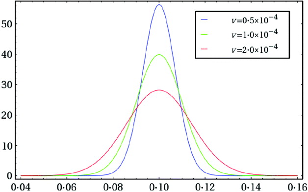
Fig. 1. Three truncated normal density functions N trunc(0·1, υ, 0·05, 0·15) with different values of υ, which can be considered as prior distributions for ε when the intended plating efficiency is ε0=0·1.
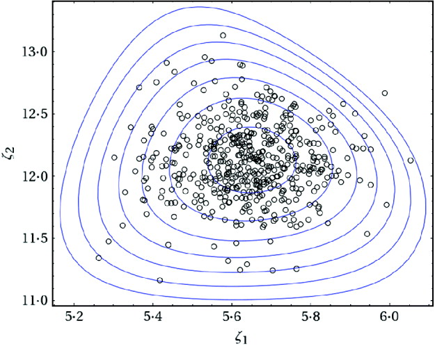
Fig. 2. Contour plot of the posterior joint density of ζ1 and ζ2 along with the last 500 draws of a simulated chain for the data given in eqn (2).
Fig. 3. Trace plot of the last 2000 ζ1 draws for the analysis of data given in eqn (2).
Fig. 4. Histogram of 5000 simulated values of the mean number of mutations m=eζ1. In this simulation for the data in eqn (2) the prior for ε was N trunc(0·1, 10−4, 0·05, 0·15).
Although the proposed method cannot be automated to the extent to which the maximum likelihood method can, the method is still simple enough for routine practical use. Sensible choice of the three tuning parameters, c, c 1 and c 2, might require time and experience on the part of the data analyst, but it is worth noting that the above simulation recipe, i.e., the length of a burn-in period and the number of iterations after the burn-in period, can tolerate a relatively wide range of values of the tuning parameters. As an illustration, we re-ran the above simulation for 1000 times. Each time we followed the same recipe, but allowed the three tuning parameters to be determined by the following equations:
where r 1, r 2 and r 3 were drawn from Uniform(0,1). The 0·025, 0·500 and 0·975 posterior quantiles are summarized in Fig. 5. The box plots clearly indicate that all the simulations led essentially to the same inference about m.
Fig. 5. The same simulation recipe described in the last section were repeated 1000 times with random tuning parameters. From the top panel to the bottom, the box plots describe the 0·025, 0·500 and 0·975 posterior quantiles, respectively, for the data given in eqn (2).
The proposed approach makes explicit a subjective ingredient in the estimator of m, which was hidden in all non-Bayesian estimators as the assumption of absolute certainty about actual plating efficiency is also subjective. The new approach offers a practical recipe for obtaining a better indication of the range of m that can be expected in view of the data at hand.
The bulk of the simulations were performed on an IBM iDataPlex machine managed by Texas A&M Supercomputing facility. The author is grateful for technical assistance provided by staff at the facility. The author also deeply appreciates the helpful comments offered by an anonymous referee.
Appendix
We propose simulating the posterior distribution of (ζ1, ζ2) by a standard ‘Metropolis within Gibbs’ algorithm (e.g. Gelman et al., Reference Gelman, Carlin, Stern and Robin2004, p. 292; Carlin & Louis, 2007, p. 141). Specifically, at the tth iteration, we
1. Draw z from Normal(0,1) and set ζ*=ζ(t−1)+c 1z.
2. Let r=min{0, h c(ζ*, ζ2(t−1))−h c(ζ1(t−1), ζ2(t−1))}.
3. Draw u from Uniform(0,1); if log u<r then set ζ1(t)=ζ*, and otherwise set ζ1(t)=ζ1(t−1).
4. Draw z from Normal(0,1) and set ζ*=ζ2(t−1)+c 2z.
5. Let r=min{0, h c(ζ1(t), ζ*)−h c(ζ1(t), ζ2(t−1))}.
6. Draw u from Uniform(0,1); if log u< r then set ζ2(t)=ζ*, and otherwise set ζ2(t)=ζ2(t−1).
Here c 1 and c 2 are two positive scale parameters chosen by trial and error to control acceptance rates.


