


Dietary intakes in the UK vary by income and socio-economic group( Reference Maguire and Monsivais 1 – Reference Darmon and Drewnowski 3 ), yet the majority of the current literature on dietary change towards healthy diets with low greenhouse gas emissions (GHGE) tends to focus on population-level studies and solutions( Reference Macdiarmid, Kyle and Horgan 4 – Reference Green, Milner and Dangour 7 ) rather than exploring the differences within the population( Reference Horgan, Perrin and Whybrow 8 ). Dietary intakes need to improve across all income groups in the population since they are not meeting the dietary recommendations for health and are contributing significantly to climate change. Dietary habits, however, vary across income group, therefore the changes needed may differ from the general population-level solutions that have been proposed. These changes include, for example, increasing consumption of fruits, vegetables and starchy foods, and reducing consumption of high-fat/high-sugar foods and animal products.
Dietary differences have been shown to be associated with the cost of food and the amount of money available to purchase food( 2 , Reference Wiggins and Alberto 9 ). In previous studies in the UK, low-income groups have reported consuming greater quantities of processed meat and sweet snacks or processed potato products (e.g. chips, crisps), while higher-income groups report consuming greater quantities of fruits, vegetables and high-fat dairy products (e.g. cheese)( Reference Maguire and Monsivais 1 , Reference Pechey, Jebb and Kelly 10 – Reference Mackenbach, Brage and Forouhi 12 ). These dietary differences across income groups have been associated with health inequalities such as obesity, type 2 diabetes and CVD( Reference Turrell and Vandevijvere 13 – Reference Drewnowski 15 ).
Cost is often perceived as a barrier to the uptake of healthy, low-GHGE diets( Reference Dixon and Isaacs 16 ). However, some studies have shown that all income groups can afford a nutritionally adequate diet without increasing cost, although this became difficult with lower food budgets( Reference Maillot, Vieux and Delaere 17 ). While a UK study found that expensive, recommended ‘healthy’ diets (i.e. Dietary Approaches to Stop Hypertension (DASH)) can have lower GHGE than cheaper, ‘unhealthier’ diets( Reference Monsivais, Scarborough and Lloyd 18 ) because they have larger amounts of lower-GHGE foods (e.g. fruits and vegetables), in contrast an Australian study showed that a typical diet actually eaten by high-income groups tends to be associated with higher GHGE than a typical diet consumed by low-income groups( Reference Reynolds, Buckley and Weinstein 19 ). This was because higher-income groups spent more on food and on some foods with higher environmental impact (e.g. meat, dairy and meals out). That study, however, did not examine the nutrient composition of the diet for health as previous studies have shown that a healthy diet does not always have a lower GHGE( Reference Vieux, Soler and Touazi 20 – Reference Vieux, Darmon and Touazi 24 ). Van Dooren( Reference van Dooren 25 ) examined GHGE and dietary requirements across Dutch sub-populations, finding those with high income and high socio-economic status had higher dietary GHGE than those on a low income and with lower socio-economic status. Van Dooren concluded that these unsustainable dietary practices of specific subgroups require dedicated transition strategies and provided examples for specific subgroups (including replacing snacks with fruit, replacing cheese with vegetables, partly replacing meat with fish, changing beverage consumption, halving the daily portion of meat).
Other barriers to dietary change include a resistance to reduce higher-GHGE foods (e.g. animal products)( Reference Dixon and Isaacs 16 , Reference Macdiarmid, Douglas and Campbell 26 ), perceived time constraints for food preparation( Reference Dixon and Isaacs 16 , Reference Jabs and Devine 27 ) and a lack of knowledge about what constitutes environmentally friendly diets( Reference Dixon and Isaacs 16 , Reference Macdiarmid, Douglas and Campbell 26 , Reference Lea and Worsley 28 ). To encourage a shift towards healthy, low-GHGE diets, these barriers could be mitigated by proposing healthy, low-GHGE diets that align more closely with current diets, to keep dietary change to a minimum.
It has been shown across European populations that change at a national dietary level towards healthy, low-GHGE diets is feasible( Reference Vieux, Perignon and Gazan 29 ). Although the changes required in the consumption of animal-based products were similar across countries and genders, other dietary changes differed (such as consumption of fish, poultry and non-liquid milk dairy). However, there is not one ideal diet or set of policy advice to move towards a lower-GHGE diet.
Change towards lower-GHGE diets is necessary to meet the UK’s GHGE reduction targets( 30 ). GHGE reductions are planned to be evenly distributed across the food system, which contributes an estimated 20 % of total UK GHGE( Reference Garnett 5 , Reference Audsley, Brander and Chatterton 31 , 32 ). Reductions in food system-associated GHGE will need to come from agriculture, processing, retail and waste management practices (supply-side change), as well as changes to diet, to successfully transition to a lower-GHGE economy( Reference Bajželj, Richards and Allwood 33 , Reference Bryngelsson, Wirsenius and Hedenus 34 ).
Household food budgets vary across the population, and this needs to be factored in to recommended dietary changes. Through dietary modelling it has been shown that healthy, affordable and low-GHGE diets are feasible at the population level( Reference Perignon, Vieux and Soler 35 – Reference Hallström, Carlsson-Kanyama and Börjesson 43 ). However, to shift to the types of diets proposed, lower-income groups would need to spend between 18 and 74 % of their total household income on food, while high-income groups would have to spend between only 6 and 10 % to achieve a similar diet( Reference Barosh, Friel and Engelhardt 44 – Reference Scott, Sutherland and Taylor 46 ).
The aim of the present study was to model healthy, low-GHGE diets that take account of current dietary habits and food budgets by income quintile. Using data from the Living Cost and Food Survey (LCFS), the study compared current household purchases, used as a proxy for diets, with optimised diets for different income groups.
Method
Study design
Linear programming was used to create low-GHGE diets that met dietary requirements and were no more expensive than existing spend on diets, while keeping the deviation from current intakes to a minimum. While linear programming has been previously used to calculate healthy, lower-GHGE and affordable diets at the population level( Reference Macdiarmid, Kyle and Horgan 4 , Reference Green, Milner and Dangour 7 , Reference Perignon, Masset and Ferrari 22 , Reference Vieux, Perignon and Gazan 29 , Reference Wilson, Nghiem and Foster 47 – Reference Milner, Green and Dangour 62 ), the present study extends the research to optimised diets for the different income quintiles and keeping dietary change to a minimum in each group. By keeping the change to a minimum, multiple diets were generated that varied the minimum amount of each food that made up the current diet. The UK’s GHGE target at the time of the study, a 57 % reduction from 1990 values by 2032, was used( 32 ). Income was based on gross income reported in LCFS; the income quintile boundaries were taken from the Office for National Statistics and generated using weighted income data to represent the UK population( 63 ). Current diets, which provide the baseline for the optimised diets, are referred to as ‘2013 diets’ herein.
Data sources
The 2013 Family Food Module of the Living Costs and Food Survey
The 2013 Family Food Module of the LCFS includes purchase data of 5144 households across the UK. Households recorded all purchases of food and drink over two weeks, including those eaten in the home and those out of the home( 2 ). The LCFS collected data on weights of all foods purchased and the amount spent (£) on each food and drink item per person per week, which was reported at the amount per individual per week level by the LCFS.
Quintile household gross income boundaries range from less than £265·18 per household per week in the lowest income (quintile 1) to more than £1077·97 per household per week in the highest (quintile 5). Individual incomes were not reported by the LCFS. Foods eaten in and outside the home were both included in the linear programming, but the foods were kept separate to allow for analysis of these differing types of purchases and food budgets.
The 337 (eaten at home) and 316 (eaten out) LCFS food categories were matched to 101 food item categories in a pre-existing data set mapped to nutrient composition and GHGE data (see Table 1 for list of the 101 food items used in the linear programming). Drinking-water was excluded from this mapping and purchased drinking-water was excluded from total spending. The nutrient composition of the foods, associated GHGE data and the purchase weights of the foods were converted to represent the edible portions (g/d)( 64 ). This included, for example, weight changes associated with cooking (e.g. rice, meat) and unavoidable wastage (e.g. banana skins). Nutrient data were taken from the National Diet and Nutrition Survey databank( Reference Bates, Lennox and Prentice 65 ). Both the LCFS and nutrient data were obtained from the UK Data Archive.
Table 1 Food groups used in the linear program, indicating if they were selected at the maximum weight limit, varied weight or at the minimum lower boundary for all linear program iterations, for all quintiles

Linear programming was used to create diets that meet dietary requirements for health and reduced greenhouse gas emissions and are affordable for different income groups using data from 5144 households in the UK Living Cost and Food Survey (2013).
* Oily fish had a minimum consumption of 19 g/d; this is a minimum increase of 400 % of 2013 consumption rates.
† Alcoholic beverages had an upper limit set at the average Living Cost and Food Survey alcohol consumption (8·9 g/d), this means there was some alcohol reduction in some diets.
‡ These foods were fixed at 100 % of their 2013 weights as they were ‘free’ foods and not purchased.
Composite meals in the LCFS were disaggregated into individual components, based on recipes from UK food composition tables and portion sizes( 64 , Reference Crawley, Millls and Patel 66 ) and cookbooks( Reference McGovern 67 – Reference Hsiung 69 ). For food categories with multiple composite dishes (e.g. takeaway and ready meals), a two-step disaggregation was used. First, composite dishes were disaggregated into the Eatwell Plate food groups proportions( Reference Whybrow, Macdiarmid and Craig 70 ). Second, within each Eatwell Plate food group, ingredients (in proportions based on the frequency of purchasing (in Scotland between 2006 and 2012) recorded by Kantar Worldpanel (www.kantarworldpanel.com/en)) were matched to one of the individual food items in the linear programming data set.
For example, for the category of takeaway meat-based meals (e.g. curries, meat pies), it was estimated that these dishes comprised 28 % protein on the Eatwell Plate. The protein category was then disaggregated into the food groups of beef (14·34 %), lamb (1·83 %), pork (1·58 %), chicken (9·38 %) and turkey (1·35 %) based on the frequency of purchase of these types of meat. The amount of each ingredient was then assigned to one of the foods in the linear programming data set.
Price data
The total spend per person was calculated by multiplying the weight of food consumed by a price vector. The price vector (£/100 g for all 101 food groups) was estimated using price and weight data from the 2013 LCFS to create an average price for each food item. Six food categories (i.e. pepper, sweetcorn, pumpkins, squash, kiwi, fried white fish and mayonnaise) did not have direct price information, and so they were matched to similar products. The LCFS supplied no food item-level price data for foods eaten out of the home; therefore, in the absence of this information, these were set the same as foods eaten at home. It is recognised that this has limitations as eating food out can be more expensive.
Greenhouse gas emissions data
GHGE data (kg CO2e/100 g product) for each of the 101 food items were based on data published by Audsley et al. ( Reference Audsley, Brander and Chatterton 31 ). These values are average emissions for production of primary food commodities up to the point of the regional distribution centre (RDC) in the UK (this excludes processing, retail, household use and waste). The RDC is described as a nominal boundary of primary production to the point of distribution for primary commodities in the UK. Audsley et al. ( Reference Audsley, Brander and Chatterton 31 ) estimate that 56 % of GHGE are accounted for up to the RDC. For foods with multiple ingredients, such as cakes, biscuits and bread, the GHGE were estimated based on the ingredients making up the food.
Audsley et al. ( Reference Audsley, Brander and Chatterton 31 ) estimated that in 1990 the GHGE of food supplied and consumed in the UK was approximately 152 Mt CO2e/year, or 7·38 kg CO2e/person per d (based on the UK population by age and sex in 1990( 71 )), or 4·14 kg CO2e/person per d to the point of the RDC. At the time of the study, the UK had targets to reduce GHGE by 57 % from 1990 values by 2032 and an 80 % reduction by 2050( 32 ). These GHGE reduction targets take account of population growth. Using the Audsley et al. 1990 value as a baseline, the 57 and 80 % GHGE reduction targets are estimated to be equivalent to 1·78 and 0·83 kg CO2e/person per d, respectively (to the point of the RDC).
Analysis: linear programming and constraints
Linear programming is a mathematical technique used to minimise or maximise a linear function, subject to a series of constraints that defines a set of linear relationships between variables and limiting resource, which has been used in other studies to optimise diets( Reference Maillot, Vieux and Delaere 17 , Reference Ward, Ward and Mantzioris 48 , Reference Buttriss, Briend and Darmon 58 , Reference Milner, Green and Dangour 62 , Reference Dantzig 72 – Reference Darmon and Drewnowski 75 ). In the present study it was used to construct nutritionally complete diets while optimising another variable (e.g. minimising GHGE), while being constrained by other factors (e.g. cost, energy, nutrients). The constraints are expressed in terms of linear combinations, with minimum requirements, upper limits or equality imposed on each item based on dietary recommendations (see Table 2 for constraints included in the models)( 76 – 80 ). In the present study, constraints comprised meeting dietary recommendations, not exceeding the budget spent on food (by quintile group) and limiting deviation from current purchases. The amount spent on each food item is based on the item as purchased, and is recorded at the household level but reported in the Family Food Report( 2 ) as amount per person per week. The objective function was the associated GHGE of the diet, which was minimised. An additional constraint for GHGE was used in later models to impose the UK GHGE reduction targets (see Table 2). More details on linear programming are given in the online supplementary material S1.
Table 2 Dietary constraints based on population-weighted dietary recommendations used in the linear programming compared with energy and nutrients reported in the 2013 diet by income quintile

Linear programming was used to create diets that meet dietary requirements for health and reduced greenhouse gas emissions and are affordable for different income groups using data from 5144 households in the UK Living Cost and Food Survey (2013).
* (a), Scientific Advisory Committee on Nutrition 2011( 76 ); (b), Department of Health 1991( 77 ); (c), Scientific Advisory Committee on Nutrition 2003( 110 ); (d), intake of alcohol in average UK household not to be increased, DEFRA 2014( 2 ); (e), Scientific Advisory Committee on Nutrition 2010( 111 ); (f), Public Health England 2014( 79 ); (g) Scientific Advisory Committee on Nutrition, Committee on Toxicity 2004 and Public Health England 2014( 79 , 80 ); (h), DEFRA 2014( 2 ); (i), Audsley et al. and UK GHGE reduction targets( Reference Audsley, Brander and Chatterton 31 , 32 ).
† Based on ≤33 % of total energy from fat.
‡ Based on ≥50 % of total energy from carbohydrate.
§ Sufficient to meet the weighted Reference Nutrient Intake.
║ Based on ≤10 % of total energy from non-milk extrinsic sugars.
¶ Based on ≤10 % of total energy from saturated fat.
** Cost constraints calculated by multiplying an average price for each food by the weight of each food purchased.
†† This constraint was not used in every model.
The energy and nutrient recommendations were weighted to reflect dietary recommendations for the current UK population (by age and sex, excluding those younger than 1 year) using the same methodology described in the LCFS( 81 ). The price constraint was set at the maximum amount that could be spent on food per day, which varied by income quintile based on its current spend.
The present study used constraints of maximum upper and variable lower boundaries for all food items to limit the deviation from the current dietary habits of each income quintile. This approach to minimise the deviation from habitual diets was used by Horgan et al.( Reference Horgan, Perrin and Whybrow 8 ) (who used fixed upper and lower bounds).
The maximum upper boundary meant that the weight of any food item from the 2013 diet could only double (200 %), which was considered a reasonable and realistic increase, and in line with previous studies( Reference Green, Milner and Dangour 7 , Reference Perignon, Masset and Ferrari 22 ). Oily fish was the exception because 2013 amounts were less than half that recommended. Alcoholic beverages could not exceed current household purchase and an upper limit was set at the average daily LCFS alcohol consumption of 8·9 g/d. This is below the national maximum recommendation for alcohol consumption( Reference Drinkaware 82 ). This meant that the amount of alcohol could not increase.
A lower boundary was the minimum deviation per food item from the 2013 diet that could be found for each modelling scenario, while meeting dietary recommendations, cost and GHGE constraints. The lower boundary was set initially at 0 % of the weight of all food items in the 2013 diet (i.e. 0 % is the greatest deviation from the diet), and the percentage increased over successive iterations of linear program runs (in steps of 1 %) until no feasible diet could be found to meet the constraints (i.e. dietary requirements, price, GHGE). For example, iteration with a lower boundary of 60 % meant that all food groups had at least 60 %, by weight, of that food in the optimised diet. The iteration that met the constraints with the highest percentage ‘lower boundary’ is referred to as the ‘final optimised diet’. This is the diet that meets all the constraints, with the smallest change from the 2013 diet that is possible using discrete linear constraints rather than an objective function, and is the diet reported in the present paper.
A population-weighted minimum fruit and vegetable constraint of 380 g/d was set, with two fruit portions and three vegetable portions to ensure a mix of fruits and vegetables in the optimised diet( 79 ). Foods with no direct cost to the household (i.e. free school milk or free school fruit) were set at fixed weights and included in the diet.
Three scenarios were run; the first included only the dietary constraints and minimum and maximum boundaries (M1), the second added the cost constraint (M2), while the final scenario rejected any solutions where the GHGE minimum was not low enough (M3). In all the scenarios GHGE were minimised.
Linear programming was carried out by using the GNU Linear Programming Kit as implemented in the Rglpk version 0.3–5 package of the R version 3.20 statistical software environment( 83 ).
Results
For all income quintiles, the linear program found a range of optimised diets with lower GHGE than the 2013 diets that met dietary and cost constraints. However, it could not find any diet to meet the 80 % GHGE reduction target with a 200 % upper limit on food weights in place.
For the average UK diet, the greater the lower boundary constraint achieved (i.e. keeping dietary change to a minimum), the higher the associated GHGE of this diet (Fig. 1(a)). Figure 1(b) shows that the average optimised diets with (M1) and without (M2) a cost constraint are the same up to until the cost constraint is met. Once the maximum cost is met, the constrained diet ‘flat lines’ in cost but increases in GHGE more quickly than the diet with no cost constraint. The cost and GHGE impacts of the diets are identical in both up to the constraint being met (at 52 %).
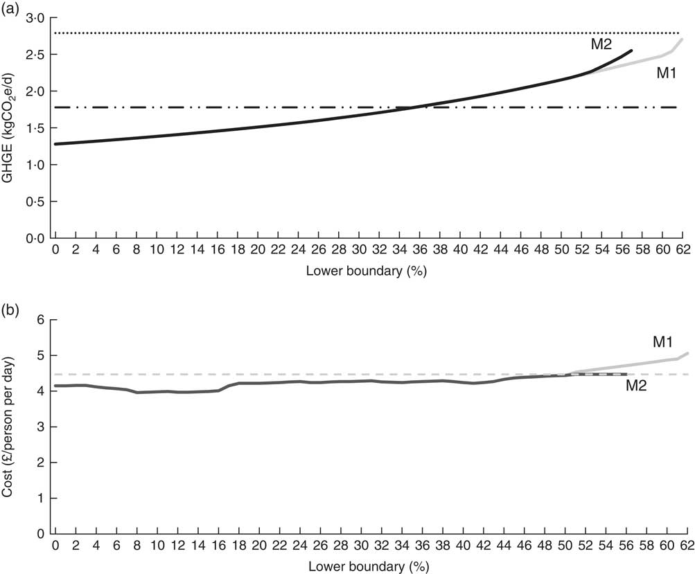
Fig. 1 Impact on greenhouse gas emissions (GHGE) and cost associated with lower boundaries of the different diets: (a) GHGE associated with different lower boundary iteration optimised diets (![]() , optimised diet, UK average, no cost constraint (M1);
, optimised diet, UK average, no cost constraint (M1); ![]() , optimised diet, UK average; cost constraint £4·47/d (M2);
, optimised diet, UK average; cost constraint £4·47/d (M2); ![]() , 2013 diet, UK average, 2·79 kg CO2e/d;
, 2013 diet, UK average, 2·79 kg CO2e/d; ![]() , 57 % GHGE reduction from 1990 level, 1·78 kg CO2e/d); (b) cost associated with different lower boundary iteration optimised diets (
, 57 % GHGE reduction from 1990 level, 1·78 kg CO2e/d); (b) cost associated with different lower boundary iteration optimised diets (![]() , optimised diet, UK average, no cost constraint (M1);
, optimised diet, UK average, no cost constraint (M1); ![]() , optimised diet, UK average; cost constraint £4·47d (M2);
, optimised diet, UK average; cost constraint £4·47d (M2); ![]() , 2013 diet, UK average, cost £4·47/d). Linear programming was used to create diets that meet dietary requirements for health and reduced GHGE and are affordable for different income groups using data from 5144 households in the UK Living Cost and Food Survey (2013)
, 2013 diet, UK average, cost £4·47/d). Linear programming was used to create diets that meet dietary requirements for health and reduced GHGE and are affordable for different income groups using data from 5144 households in the UK Living Cost and Food Survey (2013)
Income level affected the number of lower boundary iterations that could be completed by the linear program, varying from 57 to 62 % (quintile 1 to 5) when there was no cost constraint (M1) and from 53 to 60 % when cost constraint was included (M2; Table 3). This meant the higher-income group could retain more of the foods in the diet than lower-income groups. When the additional GHGE constraint was added (M3), all quintiles were reduced to similar lower boundaries (34–35 %). These final optimised diets had an average saving of £0·21/d (£0·23/d and £0·47/d in quintile 1 and 5, respectively). The greatest GHGE reduction was in the highest-income group (M3); this is due to the highest-income group having the highest 2013 GHGE and the largest capacity for reduction due to their high income and high consumption of fruits and vegetables.
Table 3 Estimated greenhouse gas emissions (GHGE) and cost of the diet by household income quintile for the 2013 diets and optimised diets for health

Linear programming was used to create diets that meet dietary requirements for health and reduced GHGE and are affordable for different income groups using data from 5144 households in the UK Living Cost and Food Survey (2013).
The lower boundary iteration refers to the minimum percentage of any food item (g/d) from the 2013 diet to be included in the optimised diet. The ‘final optimised diet’ is the iteration with the highest limit found by the linear programme to have a feasible diet.
* The energy constraint for all the optimised diets was 9200 kJ/d.
When there was no cost constraint, in order to meet the other constraints, the cost of the diets increased and GHGE decreased marginally. As more constraints were applied, the further the optimised diets departed from the 2013 diets. At the lower boundary scenario, where the cost constraint is reached (in Fig. 1 this is 52 %), the linear program begins to select cheaper foods but with higher GHGE intensity, to further increase the minimum amounts of the foods from the 2013 diet included in the optimised diet. These trade-offs lead to a divergence of the GHGE impacts for diets with and without cost constraints (as shown in Fig. 1(a) and (b) above the 52 % lower boundary). In Fig. 1(b) this divergence can also be observed, with the daily price of the cost-constrained diet ‘flat lining’ at £4·47 from the lower bound of 51 % (2·18 kg CO2e/d) to 57 % (2·55 kg CO2e/d), while the diet without a price constraint continues to increase to the lower bound of 62 % (£5·06/d and 2·70 kg CO2e/d). This illustrates a trade-off being made between higher-cost diets and healthy, lower-GHGE diets. At greater deviation from the current diet (i.e. at lower bounds), the diets cost less than the current spending.
The variability of GHGE in the 2013 and final optimised diets is due to the different dietary composition and cost constraints of each quintile. For example, in 2013, the lowest income quintiles purchased less fruits and vegetables and different types of red and processed meats, while higher income quintiles purchased more dairy in the 2013 diets. These initial differences carried over to the optimised diets because of the lower boundary constraint. Detailed diets for all lower boundaries are provided in the online supplementary material S2 (Supplemental Tables 1–7).
Substantial dietary change must occur in all income quintiles to meet the UK’s 2032 GHGE reduction target of 57 %, with fifty-eight of the 101 foods reduced to 34–35 % of their 2013 diet weights and twenty-nine foods double their 2013 diet weights (Table 4). As shown in Table 1, there were specific food items for all linear program iterations, for all quintiles, that were maximised or minimised, i.e. oily fish was quadrupled compared with 2013 diets in all quintile groups. While differences were seen between income groups in the amounts and types of individual foods that needed to change, the overall direction of dietary change needed was similar in all income groups: increase fruit, vegetables and starchy foods; reduce animal products, non-alcoholic beverages and high-fat/high-sugar foods. The food groups where the magnitude of change between quintile groups was highest included a greater reduction in alcohol in higher quintile groups and in high-fat/high-sugar foods and milk in lower quintile groups. A greater increase in fruit, vegetables and starchy foods was observed in lower quintile groups. In optimised diets GHGE differences between quintile groups mostly decreased as they shifted towards similar diets as a result of the optimisation. Some food categories (e.g. cereals) had increases in differences in GHGE between quintiles due to changes in the types/quantities of foods purchased (Table 4). Similarly, the difference between quintile groups reduced for fruit and vegetables and seafood because of differences in the original diets.
Table 4 Food purchases by household income quintile for the 2013 diets and optimised diets with cost constraint and greenhouse gas emission (GHGE) target of 1·78 kg CO2e/person per d

* Total meat also includes red meat, white meat, processed meat and liver.
† The weights (g) of these food categories are similar; however, there is difference in the GHGE between quintiles due to the differing composition of each quintile’s diet.
Results show that there is a greater than 20 % difference in GHGE between the lowest and highest GHGE quintiles for the food categories of rice, potatoes, fruits and vegetables, milk, beans, pulses, nuts, seeds, alcoholic beverages, low-calorie/sugar non-alcoholic beverages and hot beverages in 2013 diets. GHGE differences are not specifically linked to income, with the highest and lowest GHGE per category not mapping directly to income quintiles for all foods. Further information on GHGE differences can be found in online supplementary material S4 (Supplemental Tables 10 and 11).
Discussion
The present study shows that all income quintiles’ diets must change in broadly similar directions, with some variation resulting from differences in the foods contributing to GHGE in the 2013 diets. The degree of possible dietary change in each quintile was restricted by the amount of money available to purchase food and the composition of the 2013 diet. The highest income quintile achieved an optimised diet and retained greater amounts of its 2013 diet than did the lower income quintiles, but was also able to spend more on its diet. If the highest income quintile preserved the same amount of its 2013 diet as lower income quintiles, it achieved lower GHGE (Fig. 1). This result confirms the existence of trade-offs to balance healthy, low-cost and low-GHGE diets observed in other studies( Reference Monsivais, Scarborough and Lloyd 18 ), and illustrates that the trade-offs shift with income, as higher incomes can buy their way out of the trade-off until cost is a constraint (Table 3). The existence of trade-offs across income implies that attention should be given to developing interventions and dietary policies that can be achievable and effective for both lower and higher income quintiles.
The GHGE contribution of specific food categories differed across income quintiles in the 2013 and optimised diets. This is due to the 2013 dietary habits of each income quintile differing (and thus constraining the optimised diets). For example, although amounts of fruits and vegetables increased in all optimised diets, lower income quintiles consumed less fruits and vegetables in 2013 (in number of types and absolute weight) and so were constrained in the types and quantities of fruits and vegetables available in optimised diets. This is similar to the finding (at a sub-national level) that low-GHGE diets differed across European national diets due to current dietary habits( Reference Vieux, Perignon and Gazan 29 ).
Many of these differences between quintiles are passed through into the optimised diets. Retaining these dietary differences in optimised diets illustrates that population-level modelling studies have missed the distinction that healthy sustainable diets will contain different foods in different quantities at high and low incomes. This is particularly relevant as the food categories that have variations between quintiles feature in current healthy and sustainable eating guidelines( Reference Fischer and Garnett 84 – Reference van ’t Veer, Poppe and Fresco 89 ) (i.e. increasing fruits and vegetables or reducing animal products). Shifting to the more sustainable healthy diet may result in different impacts for different income quintiles. This is significant when discussing the types of foods eaten within each category, with lower-income groups eating a smaller range of fruit and vegetables and different types and weights of processed meats. If population studies alone are used to design interventions this could mean only larger dietary changes are advised, such as changing what is consumed to new, more sustainable, foods; trading in a portion of meat for a portion of fish, for example( Reference van Dooren 25 , Reference van Dooren, Keuchenius and de Vries 90 ). Introducing or trading to new foods may not prove as effective as tailored advice that shifts amounts of what is already eaten, but may be seen as more achievable as deviation from current diets is less.
Our results suggest that, at an aggregated food group level, population modelling in some cases is sufficient for some general food groups and categories. For example, the largest GHGE contributor in all diets was the food group of red meat: the 2013 amounts purchased by each quintile and the reductions required in all diets are similar, implying a population-level (society-wide) dietary change is required, rather than a change at one specific quintile level. However, the study highlights that the types of red (and processed) meat reduction is different for each quintile. For example, the consumption (and associated GHGE) of beef, lamb and pork is highest in quintile 1, while quintile 2 has the highest consumption of ham and quintile 5 has the highest consumption of chicken and bacon. Shifting to sustainable consumption patterns will involve different decisions for each quintile as well as population-level shifts of social norms and practices. Interventions and policy must recognise the differences in diets throughout society and provide advice for shifting towards realistic, healthy, low-GHGE diets for these different sectors of the population. The linear program could not find a diet that met the UK’s 2050 GHGE reduction target of 80 % with the constraints used. This is consistent with previous population studies that show GHGE reductions above 74 % were not possible no matter the deviation from the diet( Reference Perignon, Masset and Ferrari 22 ), while up to 60 % GHGE reductions were possible only if some foods deviate from the current diet by up to 200 %( Reference Green, Milner and Dangour 7 ). In the present paper, GHGE reductions were modelled from the demand side, with no changes to the GHGE intensities of food products, or the food system (supply side) via new technologies or increases in efficiency. If the currently unobtainable 2050 GHGE reduction target of 80 % is to be met, change from both demand and supply sides will be required( Reference Bajželj, Richards and Allwood 33 , Reference Bryngelsson, Wirsenius and Hedenus 34 ). However, it is also unknown how diets may change over the next few decades. The present study used a low-GHGE diet as a proxy for a sustainable diet, but it is recognised that there are other indicators of sustainability such as water, waste, land or energy use that could be included. Further research could analyse the trade-offs between these different diets in different income groups.
The optimised diets save between 18p and 47p per day across income quintiles. However, studies have shown that reducing dietary cost can result in rebound effects, where money saved in one part of the household budget (e.g. food) is spent on more GHGE-intensive items elsewhere (e.g. travel, entertainment)( Reference Chitnis, Sorrell and Druckman 91 – Reference Sorrell and Dimitropoulos 94 ). To reduce rebound effects, dietary change must be accompanied by broader transitions in consumption to a healthier, lower-GHGE lifestyle.
The monetary savings of the diet represent changes in energy to cost density, and energy to weight density, with all increasing the energy from the 2013 levels to 9250 kJ. It is well recognised that self-reported dietary records tend to be lower than actual consumption, or even requirements( Reference Stubbs, O’Reilly and Whybrow 95 ). Purchase data may be similarly under-reported( Reference Harper and Hallsworth 96 – 98 ). This increase in energy is a direct result of the constraints used, with the 2013 diets having lower energy values than estimated requirements. Additional linear program runs were carried out with energy constraints matched to 2013 energy values, and the results of these were that similar dietary shifts were required as in optimised diets. However, the cost of the final optimised diet decreased (to between £3·99 (quintile 1) and £4·10 (quintile 5); see cells K41 to O41 in the online supplementary material S3) and the lower boundary reached increased (40–42 %). Furthermore, quintiles 3 and 5 did not meet their cost constraint for any diet, with health constraints taking effect first. This implies that the fixed energy constraint forced the linear program to purchase more healthy and sustainable foods that cost more.
The present study adds to the growing evidence that income quintiles have diets that are associated with differing amounts of GHGE emissions. Previously Reynolds et al. ( Reference Reynolds, Piantadosi and Buckley 99 ) and Van Dooren et al. ( Reference van Dooren 25 ) have found 66 and 9 % GHGE differences, respectively, between high- and low-income diet-related GHGE. The baseline difference of 3 % in our study is smaller than previous studies, possibly because of a greater similarity of diets across the UK population. The larger GHGE impacts of Dutch and Australian diets can be explained by the differences in household diet composition between countries, such as higher consumptions of meat, poultry, fruit and discretionary foods( Reference van Dooren 25 , Reference van Dooren, Keuchenius and de Vries 90 , Reference Hadjikakou 100 , Reference Hendrie, Baird and Ridoutt 101 ). All studies however agree that moving towards sustainable diets will impact income quintiles in different ways due to the different income-based dietary habits. A recent US study has also looked at different households and GHGE, finding higher-GHGE diets correlated with higher spending patterns( Reference Boehm, Wilde and Ver 102 ). However, the paper analysed GHGE quintiles, not income quintiles, and did not perform any optimised diet modelling.
The types of foods selected for increase and reduction are consistent with previous population-level linear programming studies( Reference Green, Milner and Dangour 7 , Reference Perignon, Masset and Ferrari 22 , Reference van Dooren, Tyszler and Kramer 49 , Reference Donati, Menozzi and Zighetti 52 ), with starchy food, fish, fruit and vegetable consumption increasing to replace the decreases in animal products and high-fat/high-sugar foods. This is in part driven by food-based guidelines, such as for fruits, vegetables, fish and red meat. However, this is not consistent with current dietary trends where purchases of starchy foods have been decreasing since 2010( 2 ), while the consumption of fish, fruits and vegetables is static( 2 ). Encouraging increased consumption of these foods will pose its own set of challenges. Current dietary trends indicate reduction in meat consumption, particularly red meat( 2 ), which are consistent with the recommended direction of travel, but to meet GHGE targets, reduction needs to be accelerated.
The data used in the present study have some limitations. First, the LCFS is a purchase-based survey at the household level, with no adjustment for avoidable food waste or account of which household member consumes the food( Reference Burgon 103 ). Future research could incorporate average avoidable waste (i.e. food waste that would be edible) fractions into the linear program as per WRAP or Food Standards Scotland data( Reference Barton, Masson and Wrieden 104 , 105 ).
Second, the disaggregation of composite dishes into raw ingredients means that the edible weights presented in Table 3 are in total 1·1 kg/week (~9 %) higher than the purchased weights in the LCFS. Furthermore, although our composite dishes were disaggregated to component food items using standardised recipes, this may not represent the full range of dishes purchased. Both these factors could affect the energy density and processed/fresh food composition of the optimised diets.
Third, the prices used are an average price for each food item, calculated using average price paid and average weight purchased for each food item from the 2013 LCFS. Although commonly used in dietary modelling( Reference Donati, Menozzi and Zighetti 52 , Reference Darmon, Ferguson and Briend 106 , Reference Timmins, Morris and Hulme 107 ), different income quintiles may purchase similar foods at different price points. This can lead to underestimating diet cost in high income quintiles and overestimating in low income quintiles. The former was supplied as raw data from the LCFS, while the latter is calculated by multiplying the average prices of food items by the weights from the LCFS. As shown in Fig. 1 and Table 3, cost constraints did not take effect until the 47 % (quintile 1) to 54 % (quintile 5) lower boundary scenario. Changes to food prices would result in this constraint coming into effect earlier and further modifying the optimised diet. Future research could use individual prices, and optimise each diet per quintile’s average price paid, rather than at a population average.
Fourth, due to insufficient information regarding the price of food eaten out of the home, prices for foods eaten in the home were used throughout. The result of this was that the absolute spend per household was lower than in the LCFS, but the ratio of spending (and prices) was kept constant. Although the proportion of food purchased outside the home is not large (only 10 % of total energy and 11 % of the associated GHGE), this is important to note as foods eaten out of home are typically higher in cost and the types and quantity of foods eaten outside the home change with income (higher-income households purchasing greater amounts of food outside the house than lower-income households), with the average UK household spending 30 % of its food and drink spending outside the home in 2013. The models were run excluding eating out of home, with similar results (see supplementary material S3, Supplemental Tables 8 and 9). Eat-out costs results should be taken as minimum cost and could be higher for the reasons stated above. Further research is needed into the sustainability and health implications of food eaten away from home.
Fifth, the method used to keep dietary change to a minimum is a slightly crude percentage deviation to the current diet. To achieve a closer match to the current diet, a modified objective function focused on keeping dietary change to a minimum could be used in future research.
In addition, the optimised diets found in the present study are based on population-level food purchase data and so are not suggested as diets on an individual, daily basis. To create individual diets that could be realistically followed, individual diets from the LCFS could be modelled by a similar method to Horgan et al. ( Reference Horgan, Perrin and Whybrow 8 ). In the current study gross income was used rather than equivalised income due to data availability, however equivalised income quintiles can be calculated( Reference Barton, Chambers and Anderson 108 ). It is recognised that equivalised income quintiles may alter the finding slightly because this takes account of the composition of the household. Future research could investigate the differences in results between gross and equivalised income quintiles.
Finally, there is no statistical comparison of the optimised dietary results. Although not common in the optimised dietary literature to date, this limitation could be addressed in future studies using Monte Carlo and sensitivity analysis. It is also acknowledged that there are limitations due to the precision of the GHGE data, and use of Audsley et al.’s( Reference Audsley, Brander and Chatterton 31 ) data as baseline in the present study against the percentage reduction targets may not give the exact reduction required. However, in the absence of other data these were used as the baseline for the UK diets. Future research might use Monte Carlo methods to incorporate the wider UK and global( Reference Clune, Crossin and Verghese 109 ) variability of GHGE estimations into the linear program.
Conclusion
In conclusion, the current study has modelled healthy, low-GHGE diets in each income quintile that did not exceed the current household food budget by altering the amounts of different foods (but not eliminating foods) currently consumed. The more the foods from the current (2013) diet were retained in the optimised diet, the higher was the GHGE associated with the optimised diet. It was found that although all incomes had similar total GHGE impacts, there were differences in the foods within categories consumed in both 2013 and optimised diets. The results highlight that different dietary trade-offs are needed by different income quintiles, but these are generally in the same direction to be shifts towards healthy sustainable diets. This implies that although population dietary targets are sufficient, population-level sustainable dietary advice or interventions may not produce the same effects in high- and lower-income groups. Tailored dietary advice or interventions that keep dietary change to a minimum may be more effective to shift income groups to healthy and sustainable diets.
Acknowledgements
Acknowledgements: The authors thank Amandine Perrin and Hubert Ehlert for their help writing some of the early linear programming code. Financial support: This study was funded by the Scottish Government’s Rural and Environment Science and Analytical Services Division (RESAS). RESAS had no role in the design, analysis or writing of this article. Conflict of interest: There are no conflicts of interest. Authorship: J.I.M. and G.W.H. formulated the research questions. C.J.R., J.I.M., S.W. and G.W.H. contributed to the study design and analysis. C.J.R. and J.I.M. drafted the manuscript. C.J.R. had primary responsibility for the final content. All authors contributed to the final version and read and approved the final manuscript. Ethics of human subject participation: Not applicable.
Supplementary material
To view supplementary material for this article, please visit https://doi.org/10.1017/S1368980018003774


