


Introduction
Hyperspectral imaging (also known as spectrum imaging) requires software for extracting the signatures present in every spectrum. However, commercial software available for spectrum analysis remains expensive, complicated, and often not transparent regarding the internal workings and approximations made. For user facilities, educational institutes, and other settings where multiple users on a single tool can be expected, the limited availability of software becomes the bottleneck to data analysis, user training, and throughput. The Cornell Spectrum Imager (CSI) was developed as a universal data analysis tool to be freely distributed, to run on all computers, and to minimize training. This is accomplished by using one simple interface for imaging, cathodoluminescence, Raman, Electron Energy Loss Spectroscopic (EELS), and EDX data analysis. This article demonstrates the CSI plugins for ImageJ by guiding you through the basic workflow for processing EELS maps.
Download, Install, and Execute
The software package, CSI, can be downloaded for Windows, Mac OS X, or Linux operating systems at: http://code.google.com/p/cornell-spectrum-imager (click on the downloads tab). To begin using the tool, it is easiest to download one of the installers for Windows (.exe) or Mac OS X (.dmg) that will take you through the installation. If you have an existing installation of ImageJ and understand how to edit and install plugins, the necessary CSI plugins are contained in the .zip file. ImageJ without CSI is freely available from the National Institutes of Health at: http://rsb.info.nih.gov/ij/
CSI can be launched under the Applications directory in Mac OS X or through the Start Menu in Windows. When the program loads, a menu bar with a variety of CSI shortcut icons will appear (Figure 1a). Because CSI is built on ImageJ, all of the functionality familiar to ImageJ users is also available—much of which is useful in processing spectral data. The tools provided by CSI can be found in the Plugins>CSI drop-down menu. CSI is currently distributed in 64-bit format, allowing substantial memory allocation. Users processing large datasets will need to increase the memory available to CSI in the Edit⟩Options⟩Memory & Threads drop-down menu.

Figure 1: Screenshot of CSI software (v1.4) being used to analyze EELS spectral map data. (a) Shortcut icons for manipulating the dataset, (b) additional options menu, (c) spectrum analyzer showing background subtraction, and (d) the spectral map data displayed at a particular energy loss (scroll bar displays different energies).
Open and View EELS Datasets
To load a spectral dataset, click on the open spectra shortcut icon (Figure 1a). It will handle .dm3, .ser, and other common file types—such as raw binary or tiff stacks. Alternatively, data can be loaded using DM3 Reader or TIA Reader in the Plugins⟩CSI drop-down menu, as well as options available under File⟩Import. Unfortunately, a DM4 reader is not yet available because Gatan does not currently provide information regarding this new file format.
Once your data have been opened, it becomes immediately browsable. A single EELS spectrum will appear as an intensity vs. energy plot, a linescan appears as an intensity plot of position vs. energy, and for 2D spectral maps a scrollbar allows you to browse the image at any specified energy (Figure 1d). As an example, a small atomic-resolution EELS map is provided in the /ImageJ/SampleData directory. When scrolling through the energies of an EELS map, you may wish to toggle the auto-contrast button. This swaps between the default setting of automatically viewing each slice at its optimum contrast range or viewing all slices on the same intensity scale (a * at the end of the filename in the window indicates autoscaling is disabled).
When scrolling through the energy loss maps, the signal may be dominated by one or few hot pixels caused by cosmic rays or defects in the CCD. These outliers can be removed using Process⟩Noise⟩Remove Outliers in the drop-down menu. Light noise filtering will improve EELS analysis, but if the outlier threshold is set too low, the data will become median-filtered and spatial resolution will be lost. By removing hot pixels, image contrast of the raw data will be noticeably improved.
For specimens containing chemical edges with strong jump ratios, the constituent elements in the map become immediately apparent when scrolling across an edge energy onset. However, extracting a chemical map almost always requires removing the influence of the pre-edge background containing the tails of lower-energy edges and then integrating over the selected edge's energy range [Reference Egerton1]. This is done within the Spectrum Analyzer window of CSI.
The Spectrum Analyzer
Detailed spectral data analysis is done within the Spectrum Analyzer window (Figure 1c). After your data have been loaded, you can open the analyzer with the ![]() icon or under Plugins⟩CSI⟩Spectrum Analyzer.
icon or under Plugins⟩CSI⟩Spectrum Analyzer.
The Spectrum Analyzer allows you to browse information along the spectroscopic axis—in this case, electron energy (eV). For a spectral map, you can select any pixel or average signal over a region of interest using the selection toolset ![]() . The selected region need not be square—unique shapes can be generated to select nanoparticles, atomic interfaces, or semiconductor devices. When the selected region is moved, the displayed spectrum will be updated in real time. This is useful for finding elements present in a specimen, their changes in concentrations, and any fine structure changes that may occur across an interface. The Energy Window Zoom and Energy Window Offset sliders allow the user to look at specific energy windows with more detail. Fine adjustments to the energy window can be made by either typing in a specific energy in the textbox just below or clicking the slider marker and then using the left/right arrow keys.
. The selected region need not be square—unique shapes can be generated to select nanoparticles, atomic interfaces, or semiconductor devices. When the selected region is moved, the displayed spectrum will be updated in real time. This is useful for finding elements present in a specimen, their changes in concentrations, and any fine structure changes that may occur across an interface. The Energy Window Zoom and Energy Window Offset sliders allow the user to look at specific energy windows with more detail. Fine adjustments to the energy window can be made by either typing in a specific energy in the textbox just below or clicking the slider marker and then using the left/right arrow keys.
If the spectral axis of a dataset needs recalibration, right-clicking on the spectrum analyzer allows access to Calibrate Spectral Axis. Users can calibrate by specifying the position of an identifiable feature in the spectrum, such as an ionization edge, and the channel size. Alternatively, the calibration can be accomplished by specifying the position of two features. Once a calibration approach is selected, sliders specify the energy position of the feature. Editable text boxes are used to set the feature's calibrated position or channel size. Changes are applied with the Do Calibration button.
Background Subtraction
Background extrapolation and subtraction is an integral part of EELS data analysis. This is accomplished within CSI by moving the background start and width slider bars in the Spectrum Analyzer window (Figure 1c). The corresponding background energy window is shown by two vertical green bars in the spectrum. Again, fine adjustments can be made with the left/right arrow keys or by entering specific energies in the related textbox.
Once an appropriate background window has been chosen, select the preferred fitting model by clicking on the drop-down menu just above the background sliders. Typically, this means changing the default value of no fit to the power law model, power. Additional fitting methods are also provided for more advanced analysis and other types of spectral data. In particular, we have introduced a new fitting method termed Linear Combination of Power Laws (LCPL in the fitting menu) that provides a more stable background model by fitting two power laws with fixed exponents [Reference Cueva, Hovden, Mundy, Xin and Muller2]. When spectral counts are low, LCPL outperforms traditional power-law modeling.
Immediately after a background model is selected, the background-subtracted spectrum is overlaid in white. You can scale-up this white background-subtracted spectrum by clicking Auto-scale background subtracted data in the advanced options menu (right-click anywhere on the Spectrum Analyzer window).
High-magnification spectral maps are often spatially oversampled. This is the case at atomic resolution where the pixel size is up to ten times smaller than the electron probe. For such scenarios, CSI can take advantage of the redundancy in a local background by spatially averaging the background with a gaussian described by the full-width-at-half maximum (FWHM). Click the Oversampled radio button and specify the probe's FWHM in the editable text box. Specifying a FWHM much larger than the spatial resolution can introduce artifacts such as splotching or ringing [Reference Cueva, Hovden, Mundy, Xin and Muller2].
Clicking the Background Subtract Dataset button will produce a dataset with the corresponding background subtraction performed on every pixel—or alternatively, background subtraction and edge integration can be done in a single step with the Integrate button.
Extracting Chemical Maps
With the background window specified, select the Integration Window by moving the Start and Width sliders in the Spectrum Analyzer. The corresponding integration window is shown by two vertical white bars in the spectrum (Figure 1c). Clicking the Integrate button will apply the background subtraction and edge integration on every spectrum and produce either a line scan or a chemical map. If the linescan selection is made using the region of interest selection toolset, a linescan profile of chemical intensity will be produced (Figure 2). The process can be repeated over multiple edges and the resulting maps can be combined in an RGB overlay by clicking the ![]() icon or Image⟩Color⟩Stack to RGB in the menu bar. Figure 3 shows an atomic-resolution RGB map extracted from 802 × 1024 (821,248) spectra [Reference Monkman, Adamo, Mundy, Shai, Harter, Shen, Burganov, Muller, Schlom and Shen3].
icon or Image⟩Color⟩Stack to RGB in the menu bar. Figure 3 shows an atomic-resolution RGB map extracted from 802 × 1024 (821,248) spectra [Reference Monkman, Adamo, Mundy, Shai, Harter, Shen, Burganov, Muller, Schlom and Shen3].

Figure 2: Screenshot of CSI being used to analyze an EELS spectrum spatial linescan. (a) The raw linescan data is displayed allowing selection in the spatial (vertical) direction. (b) The average EELS spectra over the selected region is displayed, and (c) background subtraction and integration can generate elemental intensity profiles.

Figure 3: RGB composition of an atomic-resolution chemical map generated by CSI. The original single-element maps are shown (left), and the resulting RGB composite is shown in color (right). (LaMnO3)6(SrMnO3)3 superlattice on SrTiO3 grown by Dr. Carolina Adamo and Prof. Darrell Schlom at Cornell University. Data acquired on NION UltraStem [Reference Monkman, Adamo, Mundy, Shai, Harter, Shen, Burganov, Muller, Schlom and Shen3].
PCA Analysis
One advanced analysis tool provided by CSI is its principal component analysis (PCA) functionality. CSI calculates the single-value decomposition over the selected integration window. If a background model has been specified, the calculation will first background subtract the data when it runs. Simply click the PCA button (Figure 1c) to see the eigenvalue maps, their corresponding eigenvectors, and the scree plot (Figure 4). PCA finds components that account for the most variability in the spectral dataset, which often corresponds to the most prominent phases or element associations. The eigenvalue tells you how “much” a particular component influences one particular spectrum. Thus, the technique can elucidate changes in the spectra that might be less obvious in the raw data [Reference Bosman, Watanabe, Alexander and Keast4, Reference Bonnet5]. For example, changes in fine structure may be contained in the 2nd or 3rd component in a PCA. The first component is restricted to describing the mean of the data unless the data are first mean-centered. By mean-centering the data (Options⟩ Do Mean Centering for PCA), the PCA analysis will better characterize smaller changes in a spectrum [Reference Pun, Ellis and Eden6]. The user can also perform a weighted PCA which, based on Poisson statistics, reduces the variance contributions from noisy regions in the spectrum (Options⟩ Weight the PCA). The scree plot displays relative variance in the data represented by each component in order to help the user determine the appropriate number of components to interpret [Reference Cueva, Hovden, Mundy, Xin and Muller2]. Although the intricacies of PCA and its interpretation are too complex for this tutorial, CSI allows easy implementation. PCA is a powerful inspection and analysis tool, however it should be used only for background-subtracted data because filtering of raw EELS data can drastically distort elemental distributions and EELS fine structure [Reference Dudeck, Couillard, Lazar, Dwyer and Botton7]. A comparison of the fine structure of the O-K edge shown in Figure 4 before and after weighted PCA is given in [Reference Mundy, Mao, Brooks, Schlom and Muller8].
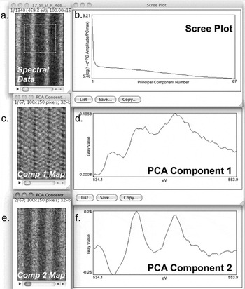
Figure 4: PCA of an EELS map (Oxygen K-Edge, LuFe2O4) showing the first two components. When running PCA on spectral data (a) in CSI, a map of all components (c or e), their shape (d or f), and a scree plot (b) is generated. The scree plot shows the declining relevance of higher-order PCA components in describing the dataset. PCA component 1 (d) is the mean O K-edge spectrum from the data set; the component 1 map (c) shows the intensity of this component in the dataset. From the scree plot (b) as well as the variation of component 2 map (e), we note that there is a physically different component 2 in the dataset, indicating that there are two different local bonding environments of O present. Although PCA component 2 (f) is not physically interpretable, the structure seen in its composition map (e) suggests local changes in the O-K fine structure. A detailed discussion of the data using other techniques is described in JA Mundy et al. [Reference Mundy, Mao, Brooks, Schlom and Muller8]. PCA allows advanced analysis of fine structure changes and peak shifts in a spectrum. Sample grown by Charles Brooks and Prof. Darrell Schlom at Cornell University.
Discussion
Cornell's Microscopy Facilities are faced with several hundred users logging over 10,000 hours on several microanalysis instruments, making the purchase of proprietary commercial software for data analysis on each instrument cost-prohibitive. CSI was created to provide an open-source platform for intuitive, advanced approaches to data analysis and processing of spectral data. Contained within CSI is a rich toolset for advanced spectral analysis beyond what is described in the present introductory tutorial. Although primarily developed for applications in electron microscopy, the open-source CSI and ImageJ platform provides an application programing interface for future algorithms or other spectroscopy communities. We encourage microscopists to use open-source software and promote open file format standards. Further documentation and updates are available at the Cornell Spectrum Imager website [9].
Acknowledgments
The authors thank Gregory Jefferis for his contributions to the DM3 reader ImageJ plugin as well as Peter Ercius for assistance with the multidimensional DM3 file formats. Without their understanding of the Gatan file formats, CSI would be greatly limited. Dr. Carolina Adamo, Charles Brooks, and Prof. Darrell Schlom provided exceptional specimens for EELS data analysis. We also acknowledge the hard work of Jo Verbeeck in developing EELSModel, another free advanced tool for those wishing to process EELS data [Reference Verbeeck and Van Aert10, 11]. Helpful feedback was also provided by Huolin L. Xin, Pinshane Huang, and Lena Fitting-Kourkoutis. Also thanks to Charles Lyman for his editorial eye. This work made use of the electron microscopy facility of the Cornell Center for Materials Research (DMR 1120296).


