


1. Introduction
Self-propulsion of microswimmers has recently drawn tremendous attention in the field of low Reynolds number microhydrodynamics because it not only occurs to many active biological and physiochemical systems but also holds the key to understanding their collective behaviours (Koch & Subramanian Reference Koch and Subramanian2011; Bechinger et al. Reference Bechinger, Di Leonardo, Löwen, Reichhardt, Volpe and Volpe2016). A common example is a swimming microorganism such as a bacterium that is self-propelled by its body movements (Lauga Reference Lauga2016). A self-motile swimmer can also be made with a catalytic Janus particle comprised of two surfaces with distinct chemical activities (Howse et al. Reference Howse, Jones, Ryan, Gough, Vafabakhsh and Golestanian2007). One widely used model for simulating the hydrodynamics of a microswimmer is the squirmer model (Lighthill Reference Lighthill1952; Blake Reference Blake1971). In this model, the squirming is generated either by small body deformations or by a prescribed tangential surface velocity along the surface of a squirmer. The simplest squirmer is a spherical squirmer. The body surface velocity for this case is often described in an axisymmetric manner with respect to the swimming direction ei of the squirmer (Ishikawa & Pedley Reference Ishikawa and Pedley2007):
 \begin{equation}u_i^s = ({e_j}{n_j}{n_i} - {e_i} ) \sum\limits_{m \ge 1} {\frac{2}{{m(m + 1)}}{B_m}} {P^{\prime}_m}({e_k}{n_k}),\end{equation}
where Pm is the Legendre polynomial of degree m with  ${P^{\prime}_m}$ being its derivative and Bm the corresponding coefficient. In (1.1), ni is the unit surface normal vector pointing into the fluid. It is common that the first two modes are sufficient to capture essential features of the squirmer (Pedley Reference Pedley2016), allowing (1.1) to take a simple form in terms of the polar angle θ measured from the swimming direction ei:
 \begin{equation}u_\theta ^s(\theta ) = {B_1}\sin \theta + {B_2}\sin \theta \cos \theta .\end{equation}
If the no-slip boundary condition is assumed at the squirmer's surface, the momentum imparted by the tangential squirming (1.2) will completely transmit into the fluid to ‘row’ the squirmer.
As indicated by (1.2), the B 1 mode describes a unidirectional tangential squirming velocity that diverges from one pole and then converges towards the other. The rowing, due to this squirming action, generates a squirming force in the direction opposite to the squirming action. This force, in turn, drives the squirmer to swim at the velocity (Lighthill Reference Lighthill1952; Blake Reference Blake1971)
 \begin{equation}{U_i} = (2/3){B_1}{e_i}.\end{equation}
The flow field generated by this mode is identified to be a source dipole, resulting from a complete cancellation between the point-force flow field arising from the squirming action and the opposite point-force flow field due to the induced translation (Blake Reference Blake1971; Pak & Lauga Reference Pak and Lauga2014).
The B 2 mode describes a symmetric extensile/contractile squirming set up by an antisymmetric body surface velocity distribution with respect to the equator at θ = π/2. For a no-slip spherical squirmer, this mode does not generate a force to propel the squirmer, rendering a stresslet (Ishikawa & Pedley Reference Ishikawa and Pedley2007)
 \begin{equation}{S_{\boldsymbol{ij}}} = 4{\rm \pi}\mu {a^2}{B_2}\left( {{e_i}{e_j} - \frac{{{\delta_{ij}}}}{3}} \right),\end{equation}
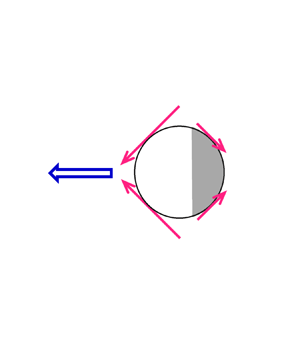
representing a symmetric force dipole to steer the squirmer of radius a in a fluid of viscosity μ. Notice that the stresslet takes the form (eiej − δij/3) that ensures that it is trace-free. It is also worth mentioning that the stresslet brought by the B 2 mode is responsible for the generic 1/r 2 far-field behaviour in the swimming flow field around the squirmer:  ${u^{\prime}_i} = {x_i}{x_j}{x_k}{S_{jk}}/8{\rm \pi}\mu {r^5}$ (Batchelor Reference Batchelor1970). Different types of swimmers described by this squirmer model can be classified according to the sign of the ratio β = B 2/B 1 between these two modes (Pedley Reference Pedley2016): β > 0 denotes a puller towed by a force self-generated ahead of its body, whereas β < 0 represents a pusher with a thrust generated behind. The particular case with β = 0 signifies a neutral squirmer. Let B 1 > 0. The sign of B 2 will determine the direction of the stresslet (either of extensile or contractile type) and hence the type of swimmer. Figure 1 illustrates how the B 1 mode and the B 2 mode in (1.2) jointly determine whether a squirmer is head-actuated or tail-actuated. It can be seen that adding the force-free B 2 mode to the thrust-providing B 1 mode causes a fore-and-aft asymmetry in the squirming force distribution, producing a biased propulsion on the front or the rear of a squirmer. This is why the direction of the stresslet is crucial in determining the type of swimmer. Furthermore, finding the stresslet of a squirmer is also essential for determining the average rheological properties of a squirmer suspension and for characterizing hydrodynamic interactions between squirmers (Ishikawa & Pedley Reference Ishikawa and Pedley2007).

Figure 1. Schematic pictures to illustrate how a unidirectional squirming through the B 1 mode and an extensile/contractile squirming through the B 2 mode act together to determine the direction and type of a homogeneous squirmer: (a) a puller and (b) a pusher. The surface velocity distribution, u s(θ), of each mode is provided with the generated squirming forces portrayed qualitatively by the red arrows. The resulting propulsion, represented by the big blue arrow, is biased towards the front to tow the squirmer ahead to act as a puller or towards the rear to push the squirmer from behind to act as a pusher. The swimming direction ei towards the right of this classical squirmer model is used to set the motion reference for the rest of this work.
The aforementioned features are given for the simplest scenario where a single spherical squirmer is swimming through an unbounded fluid under the creeping flow condition. Many extensions or variants have been made by further taking other factors into consideration. These factors include shape (Keller & Wu Reference Keller and Wu1977; Lauga & Michelin Reference Lauga and Michelin2016; Theers et al. Reference Theers, Westphal, Gompper and Winkler2016), inertia (Wang & Ardekani Reference Wang and Ardekani2012a; Chisholm et al. Reference Chisholm, Legendre, Lauga and Khair2016), unsteadiness (Wang & Ardekani Reference Wang and Ardekani2012b), nearby surface/confinement (Ishimoto & Gaffney Reference Ishimoto and Gaffney2013; Zhu, Lauga & Brandt Reference Zhu, Lauga and Brandt2013; Li & Ardekani Reference Li and Ardekani2014; Yazdi, Ardekani & Borhan Reference Yazdi, Ardekani and Borhan2014; Zöttl & Stark Reference Zöttl and Stark2014), inter-squirmer interactions (Ishikawa, Simmonds & Pedley Reference Ishikawa, Simmonds and Pedley2006; Papavassiliou & Alexander Reference Papavassiliou and Alexander2017) or their combinations (Theers et al. Reference Theers, Westphal, Qi, Winkler and Gompper2018; Ouyang & Lin Reference Ouyang and Lin2021; Ouyang et al. Reference Ouyang, Lin, Yu, Lin and Phan-Thien2022). These previous investigations basically indicate that a symmetry breaking caused by any of these factors can significantly alter the swimming characteristics of a squirmer.
In this work, we explore the swimming of a stick-slip squirmer, looking specifically at how a slip asymmetry – the symmetry-breaking mechanism that is not listed above – modifies the hydrodynamic behaviour of a self-propelled squirmer. Studying such a squirmer is motivated not only by the need for designing and controlling the motion of an active heterogeneous particle, but also by possibly new physics due to slip asymmetry in the context of the self-motile hydrodynamics.
Phenomenologically, a stick-slip squirmer can be used to model the phoretic motion of an active amphiphilic Janus particle in which the hydrophilic part is no-slip, whereas the hydrophobic part allows a small fluid slippage. An actual realization of such a particle can be achieved by using, for example, a polystyrene microsphere coated with a catalytic platinum cap (Howse et al. Reference Howse, Jones, Ryan, Gough, Vafabakhsh and Golestanian2007). Understanding how such amphiphilic particle behaves in its locomotion may provide useful guidance for how to better control and optimize its swimming performance with a stick-slip pattern.
On the fundamental side, this work is motivated by the fact that a slip asymmetry can break the symmetry of the local hydrodynamic force distribution on the surface of an otherwise no-slip or uniform-slip spherical particle (Premlata & Wei Reference Premlata and Wei2021, Reference Premlata and Wei2022). It has been shown that a stick-slip sphere can behave quite differently from a no-slip or uniform-slip sphere (Premlata & Wei Reference Premlata and Wei2021, Reference Premlata and Wei2022). For example, the former can migrate when it is placed at the centre of a purely straining flow field, whereas the latter under this same situation does not migrate at all (Premlata & Wei Reference Premlata and Wei2021). This implies that for an active stick-slip sphere, because of slip asymmetry, its swimming may not necessarily be driven solely by the unidirectional squirming of the B 1 mode; the symmetric extensile/contractile squirming of the B 2 mode can also produce an asymmetric squirming force to set the squirmer in motion. Similarly, the stresslet on such a sphere may not have to be sustained by the B 2 mode alone since a symmetric force dipole, namely a stresslet, can also form from a skewed squirming force distribution generated by the unskewed unidirectional squirming of the B 1 mode.
Another reason why we would like to study the swimming of a stick-slip squirmer is that the presence of the slip face can cause two competing effects on the squirmer. On the one hand, the squirming action will not be fully transmitted into the fluid, generating a weaker squirming force to drive the squirmer. On the other hand, the drag force on the squirmer is also diminished by the slip, which may promote the squirmer's swimming. Hence, when these two oppositely acting forces are present, it is not obvious whether the squirmer swims faster or slower compared with the no-slip counterpart.
Motivated by the above, the main theme of this work is to determine the swimming velocity Ui and the stresslet Sij for a stick-slip squirmer. We will not only examine how the two differ from the classical results of a no-slip squirmer, but also inspect how the flow field around a squirmer and its swimming performance are modified by a stick-slip disparity.
This work is organized as follows. In § 2, we will use the Lorentz reciprocal theorem to derive the formulas for Ui and Sij of a stick-slip squirmer and compute these two quantities for a given stick-slip partition. Section 3 provides pictorial mechanisms to better elucidate how asymmetric squirming forces on a stick-slip squirmer are responsible for its swimming characteristic changes. Section 4 presents our calculated Ui and Sij to demonstrate how their features are modified by a stick-slip disparity, in line with § 3. In § 5, we reveal the squirming flow structure around a stick-slip squirmer to gain more insights into how the observed swimming characteristic changes arise from a flow field point of view. We also compute the swimming power and efficiency of the squirmer to seek a possible optimization in its swimming performance with a stick-slip pattern. Final conclusions and perspectives will be made in § 6.
2. Reciprocal theorem formulation for a stick-slip spherical squirmer
We consider the motion of a two-faced spherical squirmer with a fore-and-aft partition of the stick (no-slip) and slip faces. For brevity, we call such a Janus squirmer a stick-slip squirmer. The squirmer with radius a is self-swimming at velocity Ui in an unbounded fluid of viscosity μ under the creeping flow condition. The goal here is to derive the formulas for computing the swimming velocity and the stresslet of the squirmer. Either quantity is obtained using the Lorentz reciprocal theorem (Happel & Brenner Reference Happel and Brenner1983) with the aid of the flow solution of an appropriately chosen auxiliary problem. This theorem states that two flow solutions  $({u^{\prime}_i},{\sigma ^{\prime}_{ij}})$ and $({\hat{u^{\prime}}_i},{\hat{\sigma ^{\prime}}_{ij}})$ satisfying the Stokes flow equations $\partial {u^{\prime}_i}/\partial {x_i} = \partial {\hat{u}^{\prime}_i}/\partial {x_i} = 0$ and $\partial {\sigma ^{\prime}_{ij}}/\partial {x_j} = \partial {\hat{\sigma }^{\prime}_{ij}}/\partial {x_j} = 0$ in an unbounded fluid around a particle (with the origin defined at the particle's centre) can be interrelated through the following surface integral over the particle surface (Sp) with an outward surface normal ni pointing into the fluid:
 \begin{equation}\int_{{S_p}} {{{\hat{u}^{\prime}}_i}} \textrm{ }{\sigma ^{\prime}_{ij}}{n_j}\,\textrm{d}S = \int_{{S_p}} {{{u^{\prime}}_i}} \textrm{ }{\hat{\sigma }^{\prime}_{ij}}{n_j}\,\textrm{d}S.\end{equation}
Here,  $({u^{\prime}_i},{\sigma ^{\prime}_{ij}})$ are the unknown but desired disturbance velocity and stress fields for the stick-slip problem we wish to solve; $({\hat{u^{\prime}}_i},{\hat{\sigma ^{\prime}}_{ij}})$ are the known disturbance velocity and stress fields for the auxiliary problem. These disturbance velocity and stress fields due to the presence of the particle typically decay as 1/r and 1/r 2 (or faster), respectively.
To determine the swimming velocity Ui and the stresslet Sij for the stick-slip squirmer using (2.1), we need different auxiliary problems as follows. For Ui, the auxiliary problem can be selected as the flow field around a uniform-slip sphere translating at speed  ${\hat{U}_i}$ (figure 2a). For Sij generated by the squirmer in a quiescent fluid, its calculation can be more conveniently performed using the flow field around a uniform-slip sphere held fixed at the centre of a purely straining field of strain rate $\hat{E}_{ij}^B$ (figure 2b). Below we provide separate formulations for these two problems.

Figure 2. The auxiliary problems used in the reciprocal theorem to determine the swimming characteristics of a stick-slip spherical squirmer (of radius a and slip partition angle α) in a quiescent fluid. (a) To determine the swimming velocity U driven by tangential squirming (left), the auxiliary problem considers the flow field around a uniform-slip sphere translating at speed  $\hat{\boldsymbol{U}}$ (right). (b) To determine the stresslet $\boldsymbol{\mathsf{S}}$ from the symmetric force pair (pink) as part of the squirming force generated by extensile/contractile squirming (left), we use the auxiliary flow field around a uniform-slip sphere held fixed at the centre of a purely straining field ${\hat{\boldsymbol{u}}^{\boldsymbol{B}}} = {\hat{\boldsymbol{\mathsf{E}}}^{\boldsymbol{B}}}\boldsymbol{\cdot }\boldsymbol{x}$ (right). Slip faces are indicated by the shaded regions.
2.1. Swimming velocity
We wish to establish the formula for the swimming velocity Ui of the stick-slip squirmer in terms of a prescribed tangential squirming velocity  $u_i^s$ on the squirmer's surface. Since Ui is determined by the driving squirming force $F_i^{squirm} ={-} {F_i}$ in balance with the drag force Fi on the squirmer, to determine $F_i^{squirm}$, we keep the squirmer fixed with the no-penetration condition and the slip boundary condition with a non-uniform slip length aλ(x) on its surface as
 \begin{gather}{u^{\prime}_i}{n_i} = 0,\end{gather}
 \begin{gather}{u^{\prime}_i} - u_i^s = \frac{{a\lambda (\boldsymbol{x})}}{\mu }{\sigma ^{\prime}_{jk}}{n_k}({\delta _{ij}} - {n_i}{n_j}).\end{gather}
In (2.2b), the effects of surface slip are assumed to be described by the Navier slip condition (Navier Reference Navier1823). This model states that the extent of fluid slippage can be reflected by the ratio of the slip velocity to the tangential stress. Since there is an additional tangential squirming here, the slip velocity  ${u^{\prime}_i} - u_i^s$ has to be the fluid velocity relative to the prescribed squirming velocity $u_i^s$. Therefore, slip effects will lead ${u^{\prime}_i}$ to mismatch $u_i^s$, making the latter's momentum not fully transmitted into the fluid, in contrast to ${u^{\prime}_i} = u_i^s$ in the usual no-slip situation.
For the auxiliary problem, we take a uniform-slip sphere of identical size having the constant slip length a  $\hat{\lambda }$ translating at speed ${\hat{U}_i}$ with the following boundary conditions on its surface:
 \begin{gather}({\hat{u}^{\prime}_i} - {\hat{U}_i}){n_i} = 0,\end{gather}
 \begin{gather}{\hat{u}^{\prime}_i} - {\hat{U}_i} = \frac{{a\hat{\lambda }}}{\mu }{\hat{\sigma ^{\prime}}_{jk}}{n_k}({\delta _{ij}} - {n_i}{n_j}).\end{gather}
For both problems, the velocity fields vanish as  $\textrm{|}\boldsymbol{x}\textrm{|} \to \infty$ far away from the spheres. We first extract the driving squirming force $F_i^{squirm} = \int_{{S_p}} {{{\sigma ^{\prime}}_{ij}}{n_j}} \,\textrm{d}S$ by re-arranging the left-hand side of (2.1) to
 \begin{equation}\int_{{S_p}} {{{\hat{u}^{\prime}}_i}} {\sigma ^{\prime}_{ij}}{n_j}\,\textrm{d}S = {\hat{U}_i}\int_{{S_p}} {{{\sigma ^{\prime}}_{ij}}{n_j}} \,\textrm{d}S + \int_{{S_p}} {({{\hat{u}^{\prime}}_i}} - {\hat{U}_i}){\sigma ^{\prime}_{ij}}{n_j}\,\textrm{d}S.\end{equation}
Recognizing that the velocity jump  $({\hat{u}^{\prime}_i} - {\hat{U}_i})$ on the right only acts tangentially along the sphere's surface in view of (2.3a), this jump can be replaced by the slip term in (2.3b), allowing us to recast the left-hand side of (2.1) to
 \begin{equation}\int_{{S_p}} {{{\hat{u}^{\prime}}_i}} {\sigma ^{\prime}_{ik}}{n_k}\,\textrm{d}S = {\hat{U}_i}\int_{{S_p}} {{{\sigma ^{\prime}}_{ik}}{n_k}} \,\textrm{d}S + (a/\mu )\int_{{S_p}} {\hat{\lambda }{{\hat{\sigma ^{\prime}}}_{jm}}{n_m}} ({\delta _{ij}} - {n_i}{n_j}){\sigma ^{\prime}_{ik}}{n_k}\,\textrm{d}S.\end{equation}
Similarly, for the right-hand side of (2.1), we extract the prescribed tangential squirming velocity  $u_i^s$ and replace the velocity jump $({u^{\prime}_i} - u_i^s)$ with the slip term in (2.2b):
 \begin{align}
& \int_{{S_p}} {{{u^{\prime}}_i}{{\hat{\sigma
}^{\prime}}_{ij}}{n_j}\,\textrm{d}S} = \int_{{S_p}}
{u_i^s{{\hat{\sigma }^{\prime}}_{ij}}{n_j}\,\textrm{d}S} +
\int_{{S_p}} {({{u^{\prime}}_i} - u_i^s){{\hat{\sigma
}^{\prime}}_{ik}}{n_k}\,\textrm{d}S} \nonumber\\
& \quad = \int_{{S_p}} {u_i^s{{\hat{\sigma
}^{\prime}}_{ij}}{n_j}\,\textrm{d}S} + (a/\mu )\int_{{S_p}}
{\lambda (\boldsymbol{x}){{\sigma ^{\prime}}_{jm}}{n_m}}
({\delta _{ij}} - {n_i}{n_j}){{\hat{\sigma
}^{\prime}}_{ik}}{n_k}\,\textrm{d}S.
\end{align}
\begin{align}
& \int_{{S_p}} {{{u^{\prime}}_i}{{\hat{\sigma
}^{\prime}}_{ij}}{n_j}\,\textrm{d}S} = \int_{{S_p}}
{u_i^s{{\hat{\sigma }^{\prime}}_{ij}}{n_j}\,\textrm{d}S} +
\int_{{S_p}} {({{u^{\prime}}_i} - u_i^s){{\hat{\sigma
}^{\prime}}_{ik}}{n_k}\,\textrm{d}S} \nonumber\\
& \quad = \int_{{S_p}} {u_i^s{{\hat{\sigma
}^{\prime}}_{ij}}{n_j}\,\textrm{d}S} + (a/\mu )\int_{{S_p}}
{\lambda (\boldsymbol{x}){{\sigma ^{\prime}}_{jm}}{n_m}}
({\delta _{ij}} - {n_i}{n_j}){{\hat{\sigma
}^{\prime}}_{ik}}{n_k}\,\textrm{d}S.
\end{align}Subtracting (2.5) from (2.6), we arrive at
 \begin{equation}{\hat{U}_i}F_i^{squirm} = \int_{{S_p}} {u_i^s{{\hat{\sigma }^{\prime}}_{ij}}{n_j}\,\textrm{d}S} + (a/\mu )\int_{{S_p}} {(\lambda (\boldsymbol{x}) - \hat{\lambda })} {\sigma ^{\prime}_{jm}}{n_m}({\delta _{ij}} - {n_i}{n_j}){\hat{\sigma }^{\prime}_{ik}}{n_k}\,\textrm{d}S.\end{equation}
In the above, the integral involving the slip variation  $(\lambda (\boldsymbol{x}) - \hat{\lambda })$ still contains the unknown traction ${\sigma ^{\prime}_{jm}}{n_m}$ on the squirmer's surface. For this reason, we determine $F_i^{squirm}$ approximately by assuming that the magnitude of the slip variation is small compared with the average dimensionless slip length 〈λ(x)〉 by setting $\hat{\lambda } = \langle \lambda (\boldsymbol{x})\rangle $ in (2.7), i.e.
 \begin{equation}\varepsilon \equiv |\lambda (\boldsymbol{x}) - \langle \lambda (\boldsymbol{x})\rangle |\ll 1.\end{equation}
In other words, we assume a small slip anisotropy for the squirmer to allow us to determine  $F_i^{squirm}$ accurate to O(ε) using (2.7) in which the slip length of the auxiliary uniform-slip sphere is taken to be the average slip length of the squirmer.
With (2.8), the unknown surface traction  ${\sigma ^{\prime}_{jm}}{n_m}$ in the slip variation integral can be approximated as the surface traction on a uniform-slip squirmer, $\sigma ^{\prime (0)}_{jm}{n_m}$, plus an O(ε) correction as
 \begin{equation}{\sigma ^{\prime}_{jm}}{n_m} = \sigma ^{\prime (0)}_{jm}{n_m} + O(\varepsilon ).\end{equation}
 Substituting (2.9) into (2.7) and further writing  ${\hat{\sigma }^{\prime}_{ij}}{n_j}$ in terms of the translation resistance tensor $R_{ij}^T$ obtained previously for a uniform-slip sphere (Premlata & Wei Reference Premlata and Wei2020), we obtain
 \begin{gather}{\hat{\sigma }^{\prime}_{ik}}{n_k} ={-} \mu R_{ij}^T{\hat{U}_j},\end{gather}
 \begin{gather}R_{ij}^T = \frac{1}{{a(1 + 3\hat{\lambda })}}\left( {\frac{3}{2}{\delta_{ij}} + 9\hat{\lambda }{n_i}{n_j}} \right).\end{gather}
Equation (2.7) with  $\hat{\lambda } = \langle \lambda (\boldsymbol{x})\rangle $ furnishes the squirming force for propelling a weakly stick-slip squirmer:
 \begin{equation}F_i^{squirm} ={-} \mu \int_{{S_p}} {u_k^sR_{ik}^T\,\textrm{d}S} - a\int_{{S_p}} {\mathrm{\Delta }\lambda (\boldsymbol{x})\textrm{ }} \sigma ^{\prime (0)}_{jm}{n_m}({\delta _{jk}} - {n_j}{n_k})R_{ik}^T\,\textrm{d}S,\end{equation}
where  $\Delta \lambda (\boldsymbol{x}) = \lambda (\boldsymbol{x}) - \langle \lambda (\boldsymbol{x})\rangle$ and $\hat{\lambda }$ in $R_{ij}^T$ of (2.10) is taken to be the average dimensionless slip length 〈λ(x)〉 of the stick-slip squirmer. We restate that the driving squirming force described by (2.11) is accurate up to O(ε). It actually turns out that, by comparing the results of directly solving the flow field around a stick-slip squirmer (see Appendices A and B), (2.11) is only valid when 〈λ(x)〉 is small.
To facilitate the evaluation of the slip variation term in (2.11), we use the slip boundary condition (2.3b) for the leading-order uniform-slip problem to replace the tangential stress by the velocity jump on the squirmer's surface:
 \begin{equation}\sigma
^{\prime (0)}_{jm}n_{m}({\delta _{jk}} - {n_j}{n_k}) =
\frac{\mu }{{a\langle \lambda \rangle }}(u^{\prime
\textrm{(0)}}_k -
u_k^s).\end{equation}
\begin{equation}\sigma
^{\prime (0)}_{jm}n_{m}({\delta _{jk}} - {n_j}{n_k}) =
\frac{\mu }{{a\langle \lambda \rangle }}(u^{\prime
\textrm{(0)}}_k -
u_k^s).\end{equation}So (2.11) can be rewritten as
 \begin{equation}F_i^{squirm} ={-} \mu \int_{{S_p}} {u_k^sR_{ik}^T\,\textrm{d}S} - \mu \int_{{S_p}} {\frac{{\mathrm{\Delta }\lambda (\boldsymbol{x})}}{{\langle \lambda \rangle }}\textrm{ }} (u^{\prime (0)}_k - u_k^s)R_{ik}^T\,\textrm{d}S.\end{equation}
The velocity jump  $(u^{\prime (0)}_k - u_k^s)$ can be obtained below by solving the leading-order flow field $u^{\prime (0)}_k$ in spherical polar coordinates (see Appendix A):
 \begin{equation}\frac{1}{{\langle
\lambda \rangle }}(u^{\prime (0)}_k - u_k^s) ={-} \sin
\theta \left[ {\frac{{3{B_1}}}{{1 + 3\langle \lambda
\rangle }}P_1^{\prime}(\cos \theta ) +
\frac{{(5/3){B_2}}}{{1 + 5\langle \lambda \rangle
}}P_2^{\prime}(\cos \theta )} \right]{e_\theta
}.\end{equation}
\begin{equation}\frac{1}{{\langle
\lambda \rangle }}(u^{\prime (0)}_k - u_k^s) ={-} \sin
\theta \left[ {\frac{{3{B_1}}}{{1 + 3\langle \lambda
\rangle }}P_1^{\prime}(\cos \theta ) +
\frac{{(5/3){B_2}}}{{1 + 5\langle \lambda \rangle
}}P_2^{\prime}(\cos \theta )} \right]{e_\theta
}.\end{equation}
To determine the swimming velocity Ui for the squirmer,  $F_i^{squirm}$ given by (2.13) has to be counterbalanced by the drag force Fi on the squirmer as it swims. For the latter, it can be obtained by either using the reciprocal theorem (Premlata & Wei Reference Premlata and Wei2021) or by solving the translation flow field around the squirmer (see Appendix B). This force also includes a correction due to the small slip anisotropy, taking the form (Premlata & Wei Reference Premlata and Wei2021)
 \begin{equation}{F_i} ={-} 6{\rm \pi}\mu a\textrm{ }\left( {\frac{{1 + 2\langle \lambda \rangle }}{{1 + 3\langle \lambda \rangle }}} \right)\left( {1 + \frac{{\mathcal Q}}{{(1 + 2\langle \lambda \rangle )(1 + 3\langle \lambda \rangle )}}} \right){U_i}.\end{equation}
 Here,  $\mathcal{Q}$ of O(ε) measures the strength of surface quadrupole according to the slip pattern as
 \begin{equation}{\mathrm{{\mathcal P}}_{2ij}} = \int_{{S_p}} {(\lambda (\boldsymbol{x}) - \langle \lambda (\boldsymbol{x})\rangle )(3{n_i}{n_j} - {\delta _{ij}})\,\textrm{d}S} /(4{\rm \pi}\mu {a^2}) = {\mathcal Q}(3{d_i}{d_j} - {\delta _{ij}}).\end{equation}
In (2.16), di is the stick-slip director pointing from the stick (or the less slippery) face to the slip (or the more slippery) face. This director can be either aligned to or opposite to the swimming direction ei of the squirmer in the absence of slip anisotropy. Together with the force-free condition  $F_i^{squirm} + {F_i} = 0$, we can obtain the formula for the swimming velocity of a weakly stick-slip squirmer:
 \begin{equation}{U_i} = \frac{1}{{6{\rm \pi}\mu a}}\textrm{ }\left( {\frac{{1 + 3\langle \lambda \rangle }}{{1 + 2\langle \lambda \rangle }}} \right){\left( {1 + \frac{{\mathcal Q}}{{(1 + 2\langle \lambda \rangle )(1 + 3\langle \lambda \rangle )}}} \right)^{ - 1}}F_i^{squirm},\end{equation}
where  $F_i^{squirm}$ is provided by (2.13) in which $u_i^s$, $R_{ij}^T$ and $(u^{\prime \textrm{(0)}}_i - u_i^s)$ are given by (1.2), (2.10b) and (2.14), respectively. Note that $F_i^{squirm}$ also includes an O(ε) slip variation correction due to the second term in (2.13). Using (2.17), we are able to compute Ui for the squirmer with an arbitrary axisymmetric slip pattern. For simplicity, we consider a two-faced slip pattern in terms of a partition angle α, such as that sketched in figure 2(a), to specify
 \begin{equation}\lambda
(\boldsymbol{x}) = \left\{\begin{array}{@{}ll}
{{\lambda_R}}&{\textrm{0} \le \theta \le \alpha }\\
{{\lambda_L}}&{\textrm{otherwise}} \end{array} \right..\end{equation}
\begin{equation}\lambda
(\boldsymbol{x}) = \left\{\begin{array}{@{}ll}
{{\lambda_R}}&{\textrm{0} \le \theta \le \alpha }\\
{{\lambda_L}}&{\textrm{otherwise}} \end{array} \right..\end{equation}The slip length jumps from aλR on the right face to aλL on the left face so that the average dimensionless slip length and the strength of the surface quadrupole are
 \begin{gather}\langle \lambda \rangle = (1/2)({\lambda _R} + {\lambda _L} - ({\lambda _R} - {\lambda _L})\cos \alpha ),\end{gather}
 \begin{gather}{\mathcal Q} = (1/4)({\lambda _L}-{\lambda _R})({\cos ^3}\alpha - \cos \alpha ).\end{gather}
Carrying out the integrals in (2.13) (see Appendix C), we can use (2.18) to determine the swimming velocity below after taking a small ε expansion and keeping the terms to O(ε)
 \begin{equation}{U_i} = \frac{2}{3}\textrm{ }\frac{{{e_i}}}{{1 + 2\langle \lambda \rangle }}[{B_1} + ({\lambda _L} - {\lambda _R})(\,{f_1}(\alpha ){B_1} + {f_2}(\alpha ){B_2})].\end{equation}
Here, ei is set to be the swimming direction (towards the right in figure 2a) of the squirmer without stick-slip disparity. The coefficient f 1(α) is contributed from the surface quadrupole (2.19b), and f 2(α) comes from a combination of the surface octupole and dipole (Premlata & Wei Reference Premlata and Wei2022). These coefficients vary with the stick-slip partition angle α and the average dimensionless slip length (2.19a) according to
 \begin{gather}{f_1}(\alpha ) = \frac{{1/2}}{{1 + 2\langle \lambda \rangle }}({\cos ^3}\alpha - \cos \alpha ),\end{gather}
 \begin{gather}{f_2}(\alpha ) = \frac{{1/2}}{{1 + 5\langle \lambda \rangle }}{\sin ^4}\alpha .\end{gather}
Note that α = 0 and α = π recover no-slip and uniform-slip squirmers, respectively. The swimming velocity given by (2.20) also agrees with that obtained by solving the squirming and the translation flow fields around the squirmer under the force-free condition (see (B9)–(B11) in Appendix B).
If the squirmer is uniform slip with (λL–λR) = 0, (2.20) is reduced to
 \begin{equation}{U_i} = \frac{2}{3}\textrm{ }\frac{{{B_1}}}{{1 + 2\langle \lambda \rangle }}{e_i}.\end{equation}
Here,  $\langle \lambda \rangle = 0$ recovers the no-slip result Ui = (2/3)B 1ei, determined solely by the B 1 mode (Lighthill Reference Lighthill1952; Blake Reference Blake1971). It is evident that surface slip tends to lower Ui because the less tangential stress can be transmitted from the squirming motion into the fluid. In the full slip limit with $\langle \lambda \rangle \to \infty$, there will be no swimming at all because the surface is stress-free, and no squirming force can be generated from such a surface.
If there exists a slip anisotropy on the squirmer's surface, however, (2.20) indicates that the swimming of the squirmer can be driven by an extensile/contractile squirming of the B 2 mode without involving the B 1 mode that usually provides the thrust for the swimming. Figure 3(a) illustrates physically why this can happen to a stick-slip squirmer. Even though the extensile/contractile squirming imposed by the B 2 mode is symmetric, the generated squirming forces on the stick and the slip faces are asymmetric because of stick-slip disparity. This, in turn, generates a net squirming force to set the squirmer in motion.

Figure 3. Schematic illustrations of how a stick-slip squirmer establishes its propulsion (blue arrow) when the squirming forces (pink arrows) by a single squirming mode are modified by a stick-slip disparity: (a) with only a symmetric extensile/contractile squirming by the B 2 mode, an asymmetric squirming force can be developed on the stick and the slip (in shade) faces to give net propulsion; (b) for the propulsion by a unidirectional squirming through the B 1 mode, the resulting asymmetric squirming force can be decomposed into a symmetric force dipole of strength (Fstick − Fslip) to form a stresslet plus an offset force. The direction of this disparity-induced stresslet under the B 1 mode is controlled by the stronger squirming force on the stick side.
2.2. Stresslet
We now derive the stresslet formula for a stick-slip squirmer according to (Batchelor Reference Batchelor1970)
 \begin{equation}{S_{ij}} = \int_{{S_p}} {{x_j}} {\sigma ^{\prime}_{ik}}{n_k}\,\textrm{d}S - 2\mu \int_{{S_p}} {{{u^{\prime}}_i}} {n_j}\,\textrm{d}S.\end{equation}
For convenience, we consider the squirmer held fixed in a quiescent fluid with the following boundary conditions at its surface:
 \begin{gather}{u^{\prime}_i}{n_i} = 0,\end{gather}
 \begin{gather}{u^{\prime}_i} - u_i^s = \frac{{a\lambda (\boldsymbol{x})}}{\mu }{\sigma ^{\prime}_{jk}}{n_k}({\delta _{ij}} - {n_i}{n_j}).\end{gather}
For the auxiliary problem, we consider a uniform-slip sphere of identical size with its slip length taken to be the average slip length a〈λ〉 of the stick-slip squirmer and hold it fixed at the centre of a purely straining flow field  $\hat{u}_i^B = \hat{E}_{ij}^B{x_j}$, with $\hat{E}_{ij}^B$ being the strain rate tensor. The boundary conditions at the sphere's surface are
 \begin{gather}({\hat{u}^{\prime}_i} + \hat{u}_i^B){n_i} = 0,\end{gather}
 \begin{gather}{\hat{u}^{\prime}_i} + \hat{u}_i^B = \frac{{a\langle \lambda \rangle }}{\mu }\textrm{(}{\hat{\sigma }^{\prime}_{jk}}{n_k} + \hat{\sigma }_{jk}^B{n_k}\textrm{)(}{\delta _{ij}} - {n_i}{n_j}\textrm{)},\end{gather}
where  $\hat{\sigma }_{jk}^B{n_k} = 2\mu \hat{E}_{jk}^B{n_k}$ is the surface traction exerted by the auxiliary bulk straining field.
To construct the stresslet from (2.1), we first extract the stress moment part  $\int_{{S_p}} {{x_j}{{\sigma ^{\prime}}_{ik}}{n_k}\,\textrm{d}S} $ in (2.23) from the left-hand side of (2.1), as shown by (2.26) below. Specifically, we add and subtract the stress moment from a purely straining flow field $\hat{u}_i^B = \hat{E}_{ij}^B{x_j}$. The subtracted part gives $\int_{{S_p}} {{x_j}{{\sigma ^{\prime}}_{ik}}{n_k}\,\textrm{d}S} $. In the added part, $({\hat{u}^{\prime}_i} + \hat{u}_i^B)$ can be replaced by the slip term in (2.25b). The above manipulations lead to
 \begin{align}
& \int_{{S_p}} {{{\hat{u}^{\prime}}_i}{{\sigma
^{\prime}}_{ik}}{n_k}\,\textrm{d}S} ={-} \int_{{S_p}}
{\hat{u}_i^B{{\sigma ^{\prime}}_{ik}}{n_k}\,\textrm{d}S} +
\int_{{S_p}} {({{\hat{u}^{\prime}}_i} +
\hat{u}_i^B){{\sigma ^{\prime}}_{ik}}{n_k}\,\textrm{d}S} \nonumber\\
& \quad ={-} \hat{E}_{ij}^B\int_{{S_p}} {{x_j}{{\sigma
^{\prime}}_{ik}}{n_k}\,\textrm{d}S} + \dfrac{a}{\mu
}\int_{{S_p}} {\langle \lambda \rangle ({{\hat{\sigma
}^{\prime}}_{jm}}{n_m} + \hat{\sigma }_{jm}^B{n_m})({\delta
_{ij}} - {n_i}{n_j}){{\sigma
^{\prime}}_{ik}}{n_k}\,\textrm{d}S} .
\end{align}
\begin{align}
& \int_{{S_p}} {{{\hat{u}^{\prime}}_i}{{\sigma
^{\prime}}_{ik}}{n_k}\,\textrm{d}S} ={-} \int_{{S_p}}
{\hat{u}_i^B{{\sigma ^{\prime}}_{ik}}{n_k}\,\textrm{d}S} +
\int_{{S_p}} {({{\hat{u}^{\prime}}_i} +
\hat{u}_i^B){{\sigma ^{\prime}}_{ik}}{n_k}\,\textrm{d}S} \nonumber\\
& \quad ={-} \hat{E}_{ij}^B\int_{{S_p}} {{x_j}{{\sigma
^{\prime}}_{ik}}{n_k}\,\textrm{d}S} + \dfrac{a}{\mu
}\int_{{S_p}} {\langle \lambda \rangle ({{\hat{\sigma
}^{\prime}}_{jm}}{n_m} + \hat{\sigma }_{jm}^B{n_m})({\delta
_{ij}} - {n_i}{n_j}){{\sigma
^{\prime}}_{ik}}{n_k}\,\textrm{d}S} .
\end{align} Similarly, for the velocity moment part  $- 2\mu \int_{{S_p}} {{{u^{\prime}}_i}{n_j}\,\textrm{d}S} $ of the stresslet, we can extract it from the subtracted term in the re-written form below of the right-hand side of (2.1) by working with the stress field $\hat{\sigma }_{ij}^B$ from $\hat{u}_i^B$ followed by replacing ${u^{\prime}_i}$ in the added term using (2.24b)
 \begin{align}
\int_{{S_p}} {{{u^{\prime}}_i}{{\hat{\sigma
}^{\prime}}_{ik}}{n_k}\,\textrm{d}S} &={-} \int_{{S_p}}
{{{u^{\prime}}_i}\hat{\sigma }_{ij}^B{n_j}\,\textrm{d}S} +
\int_{{S_p}} {{{u^{\prime}}_i}({{\hat{\sigma
}^{\prime}}_{ik}}{n_k} + \hat{\sigma
}_{ik}^B{n_k})\,\textrm{d}S} \nonumber\\
& \quad ={-} 2\mu \textrm{
}\hat{E}_{ij}^B\int_{{S_p}}
{{{u^{\prime}}_i}{n_j}\,\textrm{d}S} + \int_{{S_p}}
{u_i^s({{\hat{\sigma }^{\prime}}_{ik}}{n_k} + \hat{\sigma
}_{ik}^B{n_k})\,\textrm{d}S} \nonumber\\
& \quad \quad + \dfrac{a}{\mu }\int_{{S_p}} {\lambda
(\boldsymbol{x}){{\sigma
^{\prime}}_{jm}}{n_m}\textrm{(}{\delta _{ij}} -
{n_i}{n_j}\textrm{)(}{{\hat{\sigma }^{\prime}}_{ik}}{n_k} +
\hat{\sigma }_{ik}^B{n_k}\textrm{)}\,\textrm{d}S} .
\end{align}
\begin{align}
\int_{{S_p}} {{{u^{\prime}}_i}{{\hat{\sigma
}^{\prime}}_{ik}}{n_k}\,\textrm{d}S} &={-} \int_{{S_p}}
{{{u^{\prime}}_i}\hat{\sigma }_{ij}^B{n_j}\,\textrm{d}S} +
\int_{{S_p}} {{{u^{\prime}}_i}({{\hat{\sigma
}^{\prime}}_{ik}}{n_k} + \hat{\sigma
}_{ik}^B{n_k})\,\textrm{d}S} \nonumber\\
& \quad ={-} 2\mu \textrm{
}\hat{E}_{ij}^B\int_{{S_p}}
{{{u^{\prime}}_i}{n_j}\,\textrm{d}S} + \int_{{S_p}}
{u_i^s({{\hat{\sigma }^{\prime}}_{ik}}{n_k} + \hat{\sigma
}_{ik}^B{n_k})\,\textrm{d}S} \nonumber\\
& \quad \quad + \dfrac{a}{\mu }\int_{{S_p}} {\lambda
(\boldsymbol{x}){{\sigma
^{\prime}}_{jm}}{n_m}\textrm{(}{\delta _{ij}} -
{n_i}{n_j}\textrm{)(}{{\hat{\sigma }^{\prime}}_{ik}}{n_k} +
\hat{\sigma }_{ik}^B{n_k}\textrm{)}\,\textrm{d}S} .
\end{align}Combining (2.26) and (2.27) leads to
 \begin{align}
\hat{E}_{ij}^B{S_{ij}} & ={-} \int_{{S_p}}
{u_i^s({{\hat{\sigma }^{\prime}}_{ik}}{n_k} + \hat{\sigma
}_{ik}^B{n_k})\,\textrm{d}S}\nonumber \\
& \quad - \dfrac{a}{\mu
}\int_{{S_p}} {\textrm{(}\lambda (\boldsymbol{x}) - \langle
\lambda \rangle \textrm{) }{{\sigma
^{\prime}}_{jm}}{n_m}\textrm{(}{\delta _{ij}} -
{n_i}{n_j}\textrm{)(}{{\hat{\sigma }^{\prime}}_{ik}}{n_k} +
\hat{\sigma }_{ik}^B{n_k}\textrm{)}\,\textrm{d}S} .
\end{align}
\begin{align}
\hat{E}_{ij}^B{S_{ij}} & ={-} \int_{{S_p}}
{u_i^s({{\hat{\sigma }^{\prime}}_{ik}}{n_k} + \hat{\sigma
}_{ik}^B{n_k})\,\textrm{d}S}\nonumber \\
& \quad - \dfrac{a}{\mu
}\int_{{S_p}} {\textrm{(}\lambda (\boldsymbol{x}) - \langle
\lambda \rangle \textrm{) }{{\sigma
^{\prime}}_{jm}}{n_m}\textrm{(}{\delta _{ij}} -
{n_i}{n_j}\textrm{)(}{{\hat{\sigma }^{\prime}}_{ik}}{n_k} +
\hat{\sigma }_{ik}^B{n_k}\textrm{)}\,\textrm{d}S} .
\end{align}
Here, the total surface traction  $({\hat{\sigma }^{\prime}_{ik}}{n_k} + \hat{\sigma }_{ik}^B{n_k})$ can be expressed in terms of the third-rank resistance tensor $\varSigma _{qij}$ in a purely straining field (Luo & Pozrikidis Reference Luo and Pozrikidis2008):
 \begin{gather}{\hat{\sigma ^{\prime}}_{qk}}{n_k} + \hat{\sigma }_{qk}^B{n_k} = \mu {\varSigma _{qij}}\hat{E}_{ij}^B,\end{gather}
 \begin{gather}{\varSigma _{qij}} = \frac{5}{{1 + 5\langle \lambda \rangle }}({\delta _{iq}}{n_j} + 8\langle \lambda \rangle {n_q}{n_i}{n_j}).\end{gather}
Eliminating the common  $\hat{E}_{ij}^B$ in (2.28) renders the exact formula for the stresslet
 \begin{equation}{S_{ij}}
={-} \mu \int_{{S_p}} {u_q^s{\varSigma _{qij}}\,\textrm{d}S} -
a\int_{{S_p}} {\textrm{(}\lambda (\boldsymbol{x}) - \langle
\lambda \rangle \textrm{)}{{\sigma
^{\prime}}_{km}}{n_m}\textrm{(}{\delta _{kq}} -
{n_k}{n_q}\textrm{)}{\varSigma _{qij}}\,\textrm{d}S}
.\end{equation}
\begin{equation}{S_{ij}}
={-} \mu \int_{{S_p}} {u_q^s{\varSigma _{qij}}\,\textrm{d}S} -
a\int_{{S_p}} {\textrm{(}\lambda (\boldsymbol{x}) - \langle
\lambda \rangle \textrm{)}{{\sigma
^{\prime}}_{km}}{n_m}\textrm{(}{\delta _{kq}} -
{n_k}{n_q}\textrm{)}{\varSigma _{qij}}\,\textrm{d}S}
.\end{equation}
For the unknown traction  $\sigma _{km}^{\prime}{n_m}$ on the squirmer, we follow the earlier treatment and limit an O(ε) slip variation under (2.8) to approximate this traction as the uniform-slip one (2.12). The stresslet on the squirmer can then be determined accurately to O(ε) as
 \begin{equation}{S_{ij}} ={-} \mu \int_{{S_p}} {u_q^s{\varSigma _{qij}}\,\textrm{d}S} - \mu \int_{{S_p}} {\textrm{ }\frac{{\mathrm{\Delta }\lambda }}{{\langle \lambda \rangle }}\textrm{(}u^{\prime \textrm{(0)}}_q - u_q^s\textrm{)}{\varSigma _{qij}}\,\textrm{d}S} .\end{equation}
Equation (2.31) without the slip variation term is identical to the stresslet formula derived by Lauga & Michelin (Reference Lauga and Michelin2016) for no-slip squirmers. In addition, (2.31) may be applicable to an arbitrary squirmer geometry when the length scale a is taken as the characteristic length scale for a given geometry.
For the stick-slip pattern (2.18) considered here, the stresslet calculated from (2.31) (with the details given in Appendix D) is found to be
 \begin{equation}{S_{ij}} = \textrm{ }\frac{{4{\rm \pi}\mu {a^2}}}{{1 + 5\langle \lambda \rangle }}\left( {{e_i}{e_j} - \frac{{{\delta_{ij}}}}{3}} \right)[{B_2} + ({\lambda _L} - {\lambda _R})({h_1}(\alpha ){B_1} + {h_2}(\alpha ){B_2})].\end{equation}
Here, the coefficient h 1(α) comes from a combination of the surface octupole and dipole, and h 2(α) is constituted by the surface hexadecapole and quadrupole (Premlata & Wei Reference Premlata and Wei2022). These coefficients vary with the stick-slip partition angle α and the average dimensionless slip length (2.19a) according to
 \begin{gather}{h_1}(\alpha ) = \frac{{45/16}}{{1 + 3\langle \lambda \rangle }}{\sin ^4}\alpha ,\end{gather}
 \begin{gather}{h_2}(\alpha ) = \frac{{5/4}}{{1 + 5\langle \lambda \rangle }}(3{\cos ^5}\alpha - 5{\cos ^3}\alpha + 2\cos \alpha ).\end{gather}
The limiting cases α = 0 and α = π in (2.33) recover the stresslets for no-slip and uniform-slip squirmers, respectively. In the absence of slip variations with (λL–λR) = 0, (2.32) is reduced to
 \begin{equation}{S_{ij}} = \frac{{4{\rm \pi}\mu {a^2}}}{{1 + 5\langle \lambda \rangle }}\left( {{e_i}{e_j} - \frac{{{\delta_{ij}}}}{3}} \right){B_2}.\end{equation}
Also, 〈λ〉 = 0 recovers the no-slip result driven by the B 2 mode alone, as in (1.4) (Ishikawa & Pedley Reference Ishikawa and Pedley2007; Lauga & Michelin Reference Lauga and Michelin2016). Equation (2.34) reveals that the strength of the stresslet is diminished by slip effects. This is expected because less squirming work can be transmitted into the fluid when surface slip is present. In the full slip limit with  $\langle \lambda \rangle \to \infty$, the stresslet will completely vanish because no tangential stress can be generated from the squirming motion.
In contrast, for a stick-slip squirmer, its stresslet depends not only on the B 2 mode but also on the B 1 mode, as indicated by (2.32). This means that the stresslet in this case can be sustained purely by a unidirectional tangential squirming through the B 1 mode without requiring the B 2 mode, as in the no-slip case. Recall in figure 1(a) for a no-slip squirmer that no force dipole can form with the B 1 mode alone since the squirming force here is unidirectional and symmetric about the squirmer's equator at which the maximum squirming force occurs. On the contrary, for a stick-slip squirmer illustrated in figure 3(b), when it is subjected to unidirectional squirming on its surface through the B 1 mode, the tangential squirming force distribution will become skewed with a stronger (weaker) squirming force on the stick (slip) side because of stick-slip disparity. This will not only produce a net squirming force to propel the squirmer but also form a stresslet, as the asymmetric squirming force distribution can be decomposed into a symmetric force dipole plus an offset unidirectional force distribution like the B 1 mode. Note that the strength of this slip asymmetry induced stresslet is determined by the O(ε) squirming force difference between the stick and the slip faces. Also, the direction of such a stresslet is controlled by the stronger squirming force (which is on the stick side in this case). In the present case with B 1 > 0, this induced stresslet is of contractile type (with respect to the equator of the squirmer). But the overall stresslet (2.32), by combining the stresslet generated by the B 2 mode, can be of either extensile type or contractile type. This is determined by the sign of (2.32) through the parenthesis or through the stresslet coefficient  $\mathbb{S}$ (defined in (4.1b)) to indicate the direction of the stresslet. Whether a squirmer is a puller or pusher can also be classified according to the sign of $\mathbb{S}$: $\mathbb{S}$ > 0 is a puller and $\mathbb{S}$ < 0 is a pusher, true for both homogeneous and stick-slip squirmers.
3. Altering swimming characteristics by stick-slip disparity
Due to stick-slip disparity, either Ui in (2.20) or Sij in (2.32) is characterized by both the B 1 mode and the B 2 mode, signifying that the swimming features will qualitatively differ from those of a homogeneous squirmer. Before quantifying the impacts of stick-slip disparity on Ui and Sij in § 4, we provide pictorial mechanisms together with simple scaling arguments to elucidate how a stick-slip disparity modifies the squirming force distribution on a squirmer and the consequences that follow.
Recall in figure 1 that the swimming direction and the swimmer type of a no-slip squirmer are determined separately by the thrust-generating B 1 mode and the stresslet-providing B 2 mode. When the squirmer swims due to the B 1(>0) mode, a force-free stresslet created by the B 2 mode endows a skewed pulling force on the squirmer's front when the stresslet is of extensile type with β = B 2/B 1 > 0. This makes the squirmer swim as a front-actuated puller. The squirmer can also behave as a rear-actuated pusher if it engages a contractile stresslet with β = B 2/B 1 < 0. On the contrary, a stick-slip disparity can break squirming force symmetry in either driving mode so that a stick-slip squirmer can migrate with only the stresslet-providing B 2 mode and the one with only the thrust-generating B 1 mode can swim as a puller or a pusher without invoking the B 2 mode. Other than these new features, while the squirming force on the stick side is stronger than that on the slip side with a single driving mode, the relative force magnitude on the two faces may also change when both modes are acting together. This is because these forces may reinforce or counteract each other, depending on the sign of β and the direction of the stick-slip polarity, di. Hereafter, we fix B 1 > 0 and use the classical no-slip squirmer swimming in the direction ei > 0 (towards the right in figure 1) as a reference to discuss how a squirmer changes its features due to a stick-slip disparity. We also limit our discussions in this section to the cases when the stick and the slip faces are of comparable sizes to illuminate the impacts of an O(ε) slip disparity on a squirmer.
Let us first inspect how each mode influences the propulsion of a squirmer due to stick-slip disparity. Figure 4 illustrates stick-slip squirmers driven solely by the B 1 mode that is always set to generate propulsion towards the right as the tangential squirming forces on the two faces act in the same direction. When the stick-slip director (di) is aligned to the swimming direction (di = ei) as in figure 4(a), the unidirectional squirming force is weaker on the front-slip face but stronger on the rear-stick face. This makes the squirmer look as if it were propelled from behind, and hence we can categorize it as a pusher. Following figure 3(b), such an asymmetric force distribution can be decomposed into a symmetric force dipole, namely stresslet, plus another unidirectional squirming force with an offset magnitude. The strength of this disparity-induced stresslet is determined by the force difference (Fstick − Fslip) with its direction controlled by the stronger squirming force on the stick face. Specifically, it can be thought of as an induced stresslet of strength ∼εB 1 in terms of the O(ε) slip difference (λL–λR) between the two faces, but is of a contractile type ( $\mathbb{S}$ < 0) that makes the squirmer swim like a pusher. Similarly, if the stick-slip director is flipped to act against the swimming direction (dk = −ek) by placing the slip face on the left (rear) (figure 4b), the squirmer will be led by the stick face on the right (front) and swim like a puller with an extensile stresslet ( $\mathbb{S}$ > 0).

Figure 4. Schematic mechanisms for how the B 1(>0) mode can induce a stresslet due to a stick-slip disparity. Panel (a) illustrates the case with positive stick-slip polarity (di = ei) where the stick-slip director di pointing to the right-slip face is aligned with ei defined in figure 1. The squirmer is pushed more by the stronger squirming force Fstick on the rear (left) stick face to act as a pusher. Following figure 3(b), the induced stresslet of contractile type ( $\mathbb{S}$ < 0, defined in (4.1)) with its direction set by Fstick. Panel (b) shows the case with the negative stick-slip polarity (di = −ei) with the slip face on the left. The stronger Fstick on the front (right) tows the squirmer ahead to render a puller with an induced stresslet of extensile type ( $\mathbb{S}$ > 0).
To sum up the above, when a stick-slip squirmer is driven by the B 1 mode alone, its swimming velocity and induced stresslet scale as
 \begin{gather}{U_i}\sim {B_1}{e_i}[1 + O(\varepsilon )],\end{gather}
 \begin{gather}\Delta {S_{ij}}\sim{-} \varepsilon {B_1}({d_k}{e_k})\mu {a^2}({e_i}{e_i} - {\delta _{ij}}/3).\end{gather}
In (3.1a), the actual swimming velocity is slightly lower at O(ε) compared with the no-slip case's because the squirming force is reduced on the slip face. Equation (3.1b) is essentially the B 1 term in the slip variation part of (2.32). The minus sign here is to indicate the direction of the stresslet induced by the B 1 > 0 mode: it is of contractile type with  $\mathbb{S}$ < 0 when dk = ek or of extensile type with $\mathbb{S}$ > 0 when dk = −ek. This induced stresslet is a new feature due to stick-slip disparity and never occurs to a no-slip or uniform-slip squirmer.
An important consequence of (3.1b) is that an originally no-slip squirmer may switch its swimmer type when adding a slip surface, depending on whether the induced stresslet of  ${\sim} \varepsilon {B_1}\mu {a^2}$ in (3.1b) can outweigh the pre-existing stresslet of ${\sim} {B_2}\mu {a^2}$. If we add a slip cap on its front (dk = ek) as illustrated in figure 4(a), an originally no-slip puller squirmer with $\mathbb{S}$ > 0 set up by B 2 > 0 (in figure 1a) can turn into a stick-slip pusher squirmer with $\mathbb{S}$ < 0 when εB 1 > B 2 makes the total stresslet overturn its direction. However, for an originally no-slip pusher squirmer with $\mathbb{S}$ < 0 set up by B 2 < 0, the swimmer type will remain unchanged by adding a slip face on its front as the induced stresslet (3.1b) is of the same sign. However, the no-slip pusher may switch to a puller if the slip cap is placed on its rear (dk = −ek), as in figure 4(b), when the induced stresslet (3.1b) dominates the total stresslet with εB 1 > −B 2.
When the B 2 mode is acting alone, figure 5 illustrates how a stick-slip disparity imparts force asymmetry in an extensile/contractile stresslet (B 2 > 0/B 2 < 0) to drive the squirmer – a mechanism that never happens to a no-slip or uniform-slip squirmer. When a positive B 2 squirming drives on a right-slip and left-stick squirmer with dk = ek in figure 5(a), the stronger squirming force on the left-stick face surmounts the oppositely acting but weaker force on the slip face to tow the squirmer at a swimming velocity ∼εB 2 towards the left. It is noted that the squirmer moves along −ek, against the motion of the classical no-slip puller with B 2 > 0 under B 1 > 0, and hence is particularly categorized as a backward puller. If this backward propulsion by the B 2 mode is strong compared with the co-existing B 1 mode, it may diminish the swimming of a stick-slip squirmer. Similarly, when the squirming is reversed with B 2 < 0 in figure 5(b), the stronger force on the left (rear) stick face propels the squirmer from behind to make it swim like a pusher, which tends to promote the swimming of a squirmer.

Figure 5. Schematic mechanisms for how a stick-slip squirmer can be driven by the B 2 mode due to fore-and-aft asymmetric squirming forces under a stick-slip disparity. With the slip face on the right (di = ei), the stronger squirming forces on the left-stick face can drive the squirmer to act as either a backward puller when B 2 > 0 in (a), or a pusher when B 2 < 0 in (b). Similarly, if the slip face is on the left (di = −ei), the squirmer can act as a puller when B 2 > 0 in (c), or a backward pusher when B 2 < 0 in (d). In (a) and (d), the backward motion is defined with respect to ei defined in figure 1.
If the stick-slip polarity is flipped by placing the slip face on the left with dk = −ek for B 2 > 0 in figure 5(c), the stronger force on the right-stick face acts in ek and tows the squirmer like a puller. On the contrary, B 2 < 0 makes this force act backward along −ek to push the squirmer in figure 5(d), making it swim as a backward pusher. Compared with the case with a right-slip cap (dk = ek) in figures 5(a) and 5(b), figures 5(c) and 5(d) are simply the respective reversed actions without changing the swimmer type. This is a consequence of the reversibility of Stokes flow. Since the propulsion action is reversed when changing the sign of B 2, the associated promoting and diminishing swimming effects turn the opposite. That is, B 2 > 0 generates a puller action towards the left (against ek)/right (along ek) to diminish/promote the swimming of a squirmer when adding a slip face on the right/left (figures 5a and 5c). However, B 2 < 0 renders a forward/backward pusher action towards the right(along ek)/left(against ek) to enhance/depress the swimming of a squirmer when a slip face is placed on the right/left of the squirmer (figures 5b and 5d).
Summarizing the features above for a stick-slip squirmer driven by the B 2 mode alone, we recapitulate the induced swimming velocity and the stresslet in the scaling form
 \begin{gather}\Delta {U_i}\sim{-} \varepsilon {B_2}({d_k}{e_k}){e_i},\end{gather}
 \begin{gather}{S_{ij}}\sim {B_2}\mu {a^2}({e_i}{e_i} - {\delta _{ij}}/3)[1 + O(\varepsilon )].\end{gather}
Equation (3.2a) actually accounts for the slip variation term in (2.20) when B 1 = 0. The minus sign and the polarity factor (dkek) indicate that the induced swimming velocity acts in the direction opposite (parallel) to the stick-slip polarity when B 2 > 0(<0). This also implies that a stick-slip disparity can either enhance or diminish the swimming of a squirmer compared with a no-slip squirmer, depending on whether the net squirming force acts against or is aligned with the stick-slip polarity (which points in the direction from the stick face to the slip face).
After explaining the individual propulsion mechanisms for the single B 1 mode and the single B 2 mode in the presence of a stick-slip disparity, we shall discuss in what fashions the two modes will act together to propel a stick-slip squirmer. In the following analysis, we limit the discussion to the scenario where the stick and the slip faces are of comparable proportions (i.e. when α is neither close to 0 nor π). Unlike the single-mode driving that the squirming force on the stick face always exceeds the force on the slip face, owing to the induced swimming velocity (3.2a) and stresslet (3.1b), the relative force magnitude on the two faces may change when both modes are acting together. This is because the squirming force on stick/slip face from one mode can reinforce or oppose the force generated from the other mode when flipping the disparity polarity di. In figure 6, we fix B 1 > 0 and consider how an extensile/contractile squirming from the B 2 mode works with the stick-slip polarity di to determine the swimming direction and swimmer type. We shall show that the swimmer type is determined solely by the direction of the total stresslet through the sign of the stresslet coefficient  $\mathbb{S}$ defined in (4.1b): $\mathbb{S}$ > 0 is puller and $\mathbb{S}$ < 0 is pusher, applicable to both single- and mixed-mode squirming.

Figure 6. Schematic illustrations for how the B 1(>0) and the B 2(>0, <0) modes combine to set the swimming of a stick-slip squirmer whose slip face is on the right (with di = ei) or the left (with di = −ei). There are four squirming and stick-slip scenarios: (a) β = B 2/B 1 > 0, di = ei, (b) for β = B 2/B 1 < 0, di = ei, (c) for β = B 2/B 1 > 0, di = −ei and (d) for β = B 2/B 1 < 0, di = −ei. The squirming forces (pink arrows) and their magnitudes on the stick/slip faces are marked together with the sign of the stresslet coefficient ( $\mathbb{S}$) and the respective propulsion from the B 1 and the B 2 modes (hollow, solid blue arrows). When the two modes compete on the stick face in (a) and (d), the net propulsion is marked to show the winning mode; when the two modes reinforce in (b) and (c), both mode propulsion arrows are stacked. The various swimming states under these squirming and stick-slip scenarios are categorized by how β compares with the degree of stick-slip disparity ε. For a squirmer having a comparable stick-slip partition, reverse swimming can occur for |β| > 2/ε, stresslet inversion can take place for |β| < ε/2 and degraded swimming from a no-slip squirmer is found for ε/2 < |β| < 1 and 1 < |β| < 2/ε.
In figure 6(a), we first consider a squirmer having a positive stick-slip polarity (dk = ek) with a left-stick and right-slip face under B 2 > 0. The squirming force generated by the B 1 (>0) mode on the left-stick face is stronger to drive the squirmer like a pusher with an induced contractile stresslet of  $\mathbb{S}$ < 0, as illustrated in figure 4(a). The coexisting B 2 > 0 mode, on the other hand, generates an extensile squirming of $\mathbb{S}$ > 0 to drive the squirmer as a backward puller, as in figure 5(a). This shows one example for how the two driving modes can cause a counteracting effect on the swimmer type.
In terms of magnitudes of squirming forces, the squirming force generated by the B 1 (>0) mode on the stick face scales like μaB1 and is reduced to μa(1 − ε)B 1 on the slip face due to an O(ε) slip disparity. For the B 2 mode, the squirming forces on the stick and slip faces scale like −μaB 2 and μa(1 − ε)B 2, respectively. Combining the actions of these two modes, the overall squirming forces (with drag coefficient ξ ∼μa) on the rear (left) stick face and the front (right) slip face are
 \begin{gather}{F_{stick}}\sim \xi ({B_1} - {B_2}),\end{gather}
 \begin{gather}{F_{slip}}\sim \xi ({B_1} + {B_2})(1 - \varepsilon ).\end{gather}
For an originally no-slip squirmer with ε = 0 under B 1 > 0 and B 2 > 0, it is always a puller with  $\mathbb{S}$ > 0 moving towards the right along ei because the front force ∼ξ(B 1 + B 2) is always greater than the rear force ∼ξ(B 1–B 2). When a slip face is added to the squirmer's front, it skews the force distribution to modify the forces on the front slip and the back stick faces. Below we discuss how the sign and magnitude of the force on each face determine the swimming direction and the swimmer type.
When 0 < Fstick < Fslip that leads to ε/2 < β ≤ 1 (more precisely, ε/(2 − ε) < β ≤ 1) using (3.3), the squirmer is towed by the greater Fslip at the front and hence remains a puller. For such a stick-slip puller, since the pulling force on the front-slip face is weaker than that on the front face of a no-slip puller, this puller swims with a weaker pulling force and hence can be deemed as a degraded puller. But when Fstick > Fslip > 0 or β < ε/2 (more precisely, β < ε/(2 − ε)), the stronger Fstick makes the squirmer change to a pusher with  $\mathbb{S}$ < 0 due to the contractile (sign-flipped) stresslet from the B 1 squirming in figure 4(a).
However, if Fstick in (3.3a) reverses its direction to Fstick < 0 when B 2 > B 1 due to a much stronger extensile squirming by the B 2 > 0 mode, we may preserve a puller if Fslip exceeds Fstick to tow the squirmer at its front when 1 < β < 2/ε (more precisely, 1 < β < (2 − ε)/ε). Again, since the pulling force on the front is reduced due to the slip face, the squirmer swims like a degraded puller compared with the no-slip puller. Finally, when β > 2/ε, a negative Fstick can win over Fslip to give a backward puller due to the dominating B 2 mode, similar to the pulling action illustrated in figure 5(a).
As such, the four scenarios discussed above can be categorized accordingly into
(i) β < ε/2, a type-changed pusher ( $\mathbb{S}$ < 0) propelled on the rear-stick face;
(ii) ε/2 < β ≤ 1, a degraded puller (
$\mathbb{S}$ > 0) towed primarily by the force on the front-slip face with a magnitude weaker than the no-slip case;(iii) 1 < β < 2/ε, a degraded puller (
$\mathbb{S}$ > 0) with propulsion on the front-slip face weaker than the no-slip value but sufficient to overcome the backward force on the rear-stick face;(iv) β > 2/ε, a backward puller (
$\mathbb{S}$ > 0) towed on the rear-stick face.


In (ii) and (iii), the force on the front-slip side can exceed that on the rear-stick side to tow the squirmer and hence is responsible for making the total stresslet extensile type. On the contrary, in (i) and (iv), the stronger force on the rear-stick face controls the propulsion and stresslet for the squirmer and (i) can make the stresslet be of contractile type.
In summary, adding a slip face to the front of a no-slip puller squirmer can make it become a pusher because of a stresslet inversion in (i) due to a strong contractile stresslet induced by the B 1 mode (similar to the mechanism in figure 4a). The squirmer can be slowed down from a no-slip puller in (ii) and (iii) to swim like a degraded puller because of the relatively weak net propulsion force on the slip face. The squirmer can undergo a reverse swimming without changing the swimmer type in (iv) due to the backward puller action by the B 2 > 0 mode (similar to the mechanism in figure 5a).
Figure 6(b) illustrates the situation for an originally no-slip pusher with β = B 2/B 1 < 0 after adding a slip face on the squirmer's front (dk = ek). The total squirming forces on the rear (left) stick face and the front (right) slip face of the squirmer are still described by (3.3a) an (3.3b), respectively, except that the force directions for the B 2 < 0 case turn the opposite of those for the B 2 > 0 case in figure 6(a). In this case, the squirming forces on the rear-stick face for the two modes always reinforce each other towards the front, whereas those on the slip face counteract each other. As a result, Fstick always exceeds Fslip, ensuring the squirmer to be a pusher with  $\mathbb{S}$ < 0 as a no-slip pusher with β = B 2/B 1 < 0 in figure 1(b). The swimming state for this case can still be classified according to the direction of the squirming force Fslip on the slip side. When |β| < 1, Fslip follows the B 1-generated thrust towards ei. The total squirming force on this B 1-dominating front-slip pusher is ${F_{slip}} + {F_{stick}}\sim \xi {B_1}[2 - \varepsilon (1 + \beta )]$ from (3.3) and merely slightly weaker than that of ∼2ξB 1 on a no-slip pusher when −β < 1. So this pusher can be thought of as a regular pusher. On the other hand, −β > 1 leads to Fslip < 0 acting along −ei. Compared with a no-slip pusher with the total squirming force ∼−2ξB 1β(>0), the total squirming force ${F_{slip}} + {F_{stick}}\sim \xi {B_1}[2 - \varepsilon (1 + \beta )]$ on this B 2(<0) dominating front-slip pusher can be considerably greater when β < −1. Such a force reinforcement on the rear face is a consequence of the B 2-induced pusher action at O(ε) (figure 5b) and this front-slip squirmer is thus categorized as an enhanced pusher.
When the stick-slip polarity is flipped (dk = −ek) to act against the B 1 > 0 squirming in figures 6(c) and 6(d), similar force counteracting or reinforcing effects due to the coexisting B 2 mode also occur. Here, the B 1 mode generates unidirectional squirming forces on the rear (left) slip face of strength ξB 1(1 − ε) and on the front (right) stick face of strength ξB 1. The squirmer driven by this mode alone acts like a puller (see figure 4b). For the B 2 mode, it imposes asymmetric extensile/contractile squirming forces with the respective strength −ξB 2(1 − ε) and ξB 2 on the rear-slip face and the front-stick face, making the squirmer act like a backward pusher (see figure 5d). Therefore, the total squirming forces on the rear-slip face and the front-stick face are
 \begin{gather}{F_{slip}}\sim \xi ({B_1} - {B_2})(1 - \varepsilon );\end{gather}
 \begin{gather}{F_{stick}}\sim \xi ({B_1} + {B_2}).\end{gather}
With β = B 2/B 1 > 0 in figure 6(c), the squirming forces by the two modes on the front-stick face reinforce each other. So Fstick always exceeds Fslip to make the squirmer a puller with  $\mathbb{S}$ > 0, like a no-slip puller with β > 0. In this case, Fslip acts in the same direction as Fstick(>0) towards ei when β < 1, or against Fstick towards −ei when β > 1. Similar to figure 6(b), the swimming states between β < 1 and β > 1 for this rear-slip puller can be different, depending on whether the total squirming force ${F_{slip}} + {F_{stick}}\sim \xi {B_1}[2 - \varepsilon (1 - \beta )]$ on this puller exceeds that of ∼2ξB 1 on a no-slip puller with the same value of β. When β < 1, the former is slightly weaker than the latter, and hence this B 1-dominating rear-slip puller behaves like a regular puller. When β > 1, on the other hand, the total squirming force on this rear-slip puller can be made stronger than that on the no-slip puller due to the added slip face through the prevailing B 2 mode, thereby driving the rear-slip puller to swim faster like an enhanced puller.
With β = B 2/B 1 < 0 in figure 6(d), 0 < Fslip < Fstick or −β < ε/2 (more precisely, −β < ε/(2 − ε)) turns the originally no-slip pusher with β < 0 into a puller with  $\mathbb{S}$ > 0. However, when ${F_{slip}} > {F_{stick}} > 0$ or $\varepsilon /2 < - \beta \le 1$ (more precisely, $\varepsilon /(2 - \varepsilon ) < - \beta \le 1$), it renders a degraded pusher with $\mathbb{S}$ < 0 since it is propelled on the rear-slip face with a weaker squirming force compared with the no-slip counterpart. If a negative B 2 exceeds B 1 to reverse Fstick, we may preserve a degraded pusher if the total squirming force ${F_{slip}} + {F_{stick}}\sim \xi {B_1}[(2 - \varepsilon ) + \varepsilon \beta ] > 0$ when 1 < −β < 2/ε, but may end up with a backward pusher if Fslip + Fstick < 0 when −β > 2/ε. Like figure 6(a), these four scenarios can be summarized as
(i) |−β| < ε/2, a puller (
$\mathbb{S}$ > 0) towed on the front-stick face;(ii) ε/2 < |−β| ≤ 1, a degraded pusher (
$\mathbb{S}$ < 0) with a weaker thrust on the rear-slip face;(iii) 1 < |−β| < 2/ε, a degraded pusher (
$\mathbb{S}$ < 0) propelled by a weaker force on the rear-slip face;(iv) |−β| > 2/ε, a backward pusher (
$\mathbb{S}$ < 0) propelled from the front-stick face.


Hence, adding a slip face to the rear of an originally no-slip pusher squirmer can turn it into a puller in (i) due to a stresslet inversion by the B 1 mode. It swims slower in (ii) and (iii) and even reverses its swimming direction without changing the swimmer type in (iv) when the B 2 < 0 mode competes or outperforms the B 1(>0) mode to bring out its backward pusher action illustrated in figure 5(d).
In fact, all the classified swimming states in figure 6 can be summarized in a β–ε phase diagram accordingly in figures 7(a) and 7(b) for right-slip squirmers (dk = ek) and left-slip squirmers (dk = −ek), respectively. These distinct swimming states can be categorized as either counteracting propulsion or reinforcing propulsion. Counteracting propulsion means that the squirming forces on the stick face from the two modes act to oppose each other, as illustrated in figures 6(a) and 6(d). Reinforcing propulsion, on the contrary, refers to the situation when these forces act in the same direction, as seen in figures 6(b) and 6(c).

Figure 7. Swimming phase diagrams in view of β = B 2/B 1 and the degree of stick-slip disparity  $\varepsilon ({\ll} 1)$, summarizing all different swimming states in figure 6. For a stick-slip squirmer with the slip face on the right in (a), the squirmer can change the swimming characteristics by decreasing its β from a large positive value: from a backward puller, a degraded puller, a pusher, to an enhanced pusher. The squirmer experiences motion reversal at the transition condition β = 2/ε, type change at β = ε/2, stresslet enhancement for β > −1 and swimming enhancement for β < −1. Reversing the stick-slip polarity by placing a slip face on the left of a squirmer in (b), the above sequence of the swimming states will be reversed but with the puller type replaced with the pusher type. The colour shades correspond to those in figures 8 and 9.
For counteracting propulsion, there are eight swimming states: four states occur for an originally no-slip puller squirmer with β > 0 when a slip face is placed on the front (see figure 6a). The other four states happen for an originally no-slip pusher squirmer with β < 0 after a slip face is added on the rear (see figure 6d). Swimming characteristic changes can occur to a puller/pusher squirmer with the slip cap on the front/rear in two extreme regimes |β| < ε/2 and |β| > 2/ε where the O(ε) slip-asymmetry-induced effects of one mode outperforms the original effects of the other mode. As illustrated in figures 6(a) and 6(d), in the small |β| < ε/2 regime, the squirmer switches the swimmer type along with a stresslet inversion without changing the swimming direction due to the O(ε) stresslet induced by the B 1 mode. In the large |β| > 2/ε regime, the O(ε) propulsion induced by the B 2 mode on the squirmer gives rise to reverse swimming without changing the swimmer type. In the intermediate region ε/2 < |β| < 1 and 1 < |β| < 2/ε, the swimming is controlled by a greater total squirming force on the slip face. Reinforcing propulsion occurs to a pusher with β < 0 when a slip face is placed on its front (dk = ek), or to a puller with β > 0 when a slip face is added to its rear (dk = −ek). A stick-slip pusher and puller of this sort can swim faster than the no-slip counterparts when β < −1 and β > 1, respectively, due to the much amplified squirming force by the stresslet actions from the more dominant B 2 mode, as illustrated in figures 6(b) and 6(c).
As counteracting propulsion and reinforcing propulsion for a given stick-slip geometry always occur at different signs of β, figures 7(a) and 7(b) also serve as the respective swimming phase diagrams for the front-slip and the rear-slip cases as varying the value of β. For a squirmer with the front-slip face, it can be clearly seen from figure 7(a) that, as β is decreased from a very positive value to a very negative value, the squirmer can act as a backward puller, a degraded puller, a pusher and an enhanced pusher, experiencing motion reversal at the transition point β = 2/ε, type change at the transition point β = ε/2, stresslet enhancement for β > −1 and swimming enhancement for β < −1. However, if the stick-slip polarity is flipped towards the left by placing a slip face on the rear of a squirmer, the above sequence of the swimming states will be reversed but with the puller type replaced by the pusher type for each state, as shown in figure 7(b).
4. Quantifying swimming characteristic changes due to stick-slip disparity
After qualitative categorization of the rich propulsion scenarios for a stick-slip squirmer, we compute the swimming velocity Ui from (2.20) and the stresslet Sij from (2.32) to quantify the differences from those of the classical no-slip squirmer illustrated in figure 1. With the reference set to be the no-slip case, we define the swimming coefficient and the stresslet coefficient below to characterize the impacts of stick-slip disparity on Ui and Sij
 \begin{gather}{{\mathbb V}} \equiv {U_i}/{U_i}(\langle \lambda \rangle = 0) = {(1 + 2\langle \lambda \rangle )^{ - 1}}[1 + ({\lambda _L} - {\lambda _R})(\,{f_1}(\alpha ) + {f_2}(\alpha )\beta )],\end{gather}
 \begin{gather}\mathbb{{ S}} \equiv {S_{ij}}/|{S_{ij}}(\langle \lambda \rangle = 0)|= \textrm{sign}\;(\beta ){\left( {1 + 5\left\langle \lambda \right\rangle } \right)^{ - 1}}[1 + ({\lambda _L} - {\lambda _R})({h_1}(\alpha ){\beta ^{ - 1}} + {h_2}(\alpha ))].\end{gather}
 Equation (4.1a) measures the degree of swimming enhancement or diminishment with respect to the no-slip's swimming velocity Ui(〈λ〉 = 0) from (1.3) (>0 towards the right, along ei) and can change sign to signify a reverse swimming (<0 towards the left, along −ei).(4.1b) reflects how the total stresslet Sij changes its strength from the no-slip case |Sij(〈λ〉 = 0)| given in (1.4). In addition, the sign of this coefficient  $\mathbb{S}$ > 0 or $\mathbb{S}$ < 0 is to indicate a puller of extensile stresslet or a pusher of contractile stresslet, especially a possible sign change due to stresslet inversion.
Other than the average dimensionless slip strength 〈λ〉 and the slip partition α, (4.1) also indicates that swimming characteristic changes will depend crucially on the sign of (λR–λL) that sets the direction of the stick-slip polarity di with respect to the driving squirming force direction of the B 1 mode or the swimming direction ei (towards the right) of an originally no-slip squirmer. We present results according to the direction of the stick-slip polarity and examine both β = B 2/B 1 > 0 and <0 driving scenarios to quantify how the swimming behaviour of an originally no-slip squirmer is modified by an added slip face.
4.1. Positive stick-slip polarity (λR−λL) > 0 case
4.1.1. The case β = B 2/B 1 > 0
Starting with an originally no-slip puller squirmer with β = B 2/B 1 > 0, we look at how  $\mathbb{V}$ and $\mathbb{S}$ are modified by adding a slip face on its front (right) with (λR−λL) > 0. Figure 8(a) plots how $\mathbb{V}$ varies with the partition α/π of the slip face for various values of β and the corresponding plot for $\mathbb{S}$ is shown in figure 8(b).

Figure 8. Plots of how the swimming coefficient  $\mathbb{V}$ in (4.1a) and the stresslet coefficient $\mathbb{S}$ in (4.1b) vary with the partition α/π of the slip face and β = B 2/B 1 for a right-slip squirmer with (λL, λR) = (0, 0.2). Panels(a) and (b) show the results with β > 0. For a small β = 0.1, $\mathbb{V}$ decreases monotonically from the no-slip value (α/π = 0) to the uniform-slip value (α/π = 1) in (a) but the squirmer can change to a pusher with $\mathbb{S}$ < 0 due to stresslet inversion by the much stronger B 1 mode (like in figure 4a) in (b). Increasing β not only lowers $\mathbb{V}$ but also makes the squirmer return to the degraded puller state due to the backward puller action by the B 2 mode (as in figure 5a). For a large β = 10, the backward pulling can dominate to reverse its swimming direction with $\mathbb{V}$ < 0 in (a) like a backward puller with $\mathbb{S}$ > 0 in (b). Panels (c) and (d) plot $\mathbb{V}$ and $\mathbb{S}$ with β < 0 under which the squirmer always acts as a pusher. Apparent swimming enhancement from $\mathbb{V}$ < 1 to $\mathbb{V}$ > 1 by increasing |−β| is observed in (c) while $\mathbb{V}$ > 1 comes with a diminishment of $|\mathbb{S}|\ (\mathbb{S}$ < 0) in (d). The swimming states are marked according to figure 7(a).
As revealed in figure 8(a), for a small value of β such as β = 0.1 under which the B 1 mode is more dominating than the B 2 mode,  $\mathbb{V}$ remains positive and decreases monotonically with α from the no-slip value with α = 0 to the uniform-slip value with α = π. Hence, the stick-slip squirmer does not change the swimming direction. This squirmer swims slightly more slowly than the no-slip squirmer due to the swimming diminishment by the dominating B 1 mode through the f 1 term and by the drag reduction factor ${(1 + 2\langle \lambda \rangle )^{ - 1}}$ in (4.1a) due to an increase of 〈λ〉 with α according to (2.19a).
However, it is also this dominating B 1 mode that enhances the O(ε) pusher-like stresslet (of  $\mathbb{S}$ < 0) (see figure 4a) to compete with the co-existing puller stresslet (of $\mathbb{S}$ > 0) sustained by the B 2(>0) mode. When β is small, the former can even outweigh the latter into a total stresslet inversion since the slip disparity effect on $\mathbb{S}$ through (λL−λR) < 0 in (4.1b) is greatly amplified by the ${\beta ^{ - 1}}{h_1} > 0$ term from the B 1 mode. This explains why the $\mathbb{S}$-α profile at β = 0.1 resembles the profile of $({\lambda _L}\unicode{x2013}{\lambda _R}){\beta ^{ - 1}}{h_1}\sim{-} {\beta ^{ - 1}}{\sin ^4}\alpha$ to display a negative minimum at around α/π = 0.5 in figure 8(b). Increasing β decreases the magnitude of this stresslet minimum until $\mathbb{S}$ changes its sign to indicate a stresslet/swimmer-type inversion from a pusher of $\mathbb{S}$ < 0 to a puller of $\mathbb{S}$ > 0, corresponding to the type change when entering the β > ε/2 regime on the phase diagram in figure 7(a). While such a stresslet/swimmer type inversion effect due to the B 1 mode becomes sluggish by raising β for diminishing the ${\beta ^{ - 1}}{h_1}$ term in (4.1b), $\mathbb{V}$ is further slowed down in figure 8(a). This velocity diminishment is due to the amplified (λL−λR)f 2β < 0 term in (4.1a) through the O(ε) backward puller propulsion by the B 2 mode (see figure 5a). When reaching β ∼1 where the B 2 mode becomes comparable to the B 1 mode, $\mathbb{V}$ starts to display a minimum at around α/π = 0.5 due to $({\lambda _L}\unicode{x2013}{\lambda _R}){f_2}\beta \sim{-} \beta {\sin ^4}\alpha$ in (4.1a). The corresponding $\mathbb{S}$ no longer changes its sign and remains positive because the co-existing B 2-driven puller stresslet of $\mathbb{S}$ > 0 outshines the O(ε) B 1-induced pusher stresslet of $\mathbb{S}$ < 0.
For a large enough β > 1, the f 2β term from the B 2 mode dominates and amplifies the backward puller propulsion effect on the swimming velocity (4.1a) to even change its sign to reverse the swimming direction, as shown in figure 8(a). Meanwhile, the diminishment of  $\mathbb{S}$ by the B 1-induced pusher effect is reduced by increasing β so that $\mathbb{S}$ remains positive to preserve the swimmer type, as shown in figure 8(b). The dominant B 2 mode effect due to large β also explains why the $\mathbb{V}$–α profile at β = 10 in figure 8(a) resembles the profile of $({\lambda _L}\unicode{x2013}{\lambda _R}){f_2}\beta \sim{-} \beta {\sin ^4}\alpha$ to display a negative minimum at around α/π = 0.5. This corresponds to the swimming state with β > 2/ε in figure 6(a) due to counteracting propulsion, and is classified as a backward puller on the phase diagram in figure 7(a). In the regime between small and large values of β, such as 1 < β < 8, the squirmer simply swims slower than both the no-slip and uniform-slip squirmers without changing its swimming direction and swimmer type, as shown in figures 8(a) and 8(b) for $\mathbb{V}$ and $\mathbb{S}$. The squirmer in this intermediate regime behaves as a degraded puller with ε/2 < β < 2/ε on the phase diagram in figure 7(a).
As such, for a squirmer having a comparable stick-slip partition to α = π/2, we observe that  $\mathbb{V}$ changes from positive to negative when β is increased while the corresponding $\mathbb{S}$ goes from negative to positive. The opposite trends of $\mathbb{V}$ and $\mathbb{S}$ with β are the reflections of the different propulsion scenarios illustrated in figure 6(a) or on the β > 0 plane of the phase diagram in figure 7(a), which are summarized below:
(i) small 0 < β < ε/2 gives a forward pusher with
$\mathbb{V}$ > 0 and $\mathbb{S}$ < 0, where the stresslet inversion results from the dominating B 1-induced stresslet;(ii) intermediate ε/2 < β < 2/ε gives a degraded forward puller with
$\mathbb{V}$ > 0 and $\mathbb{S}$ > 0, which is just a slower squirmer of the same type as the no-slip case;(iii) large β > 2/ε gives a backward puller with
$\mathbb{V}$ < 0 and $\mathbb{S}$ > 0, where the reverse motion is a result of the winning B 2-induced counteracting propulsion.


4.1.2. The case β = B 2/B 1 < 0
Next, we consider the case of an originally no-slip pusher squirmer with β = B 2/B 1 < 0. Figures 8(c) and 8(d) present the calculated  $\mathbb{V}$ and $\mathbb{S}$ after adding a slip face on the squirmer's front (right).
Because the B 2-driven stresslet is now of contractile type with  $\mathbb{S}$ < 0, the resulting stronger squirming force on the rear-stick face acts in the same direction as that of the B 1 mode. This reinforces the rear propulsion on the stick face as in figure 6(b), and makes the squirmer swim in the same direction and type as a no-slip pusher squirmer on the β < 0 plane in figure 7(a). This propulsion reinforcement on the stick face may enhance the pusher swimming when |−β| is large enough to make the B 2 mode's effects stronger than the B 1 mode's. It can be seen from (4.1a) that the βf 2 < 0 term from the B 2 < 0 mode may outweigh the f 1 > 0 term from the B 1 mode and work with the stick-slip disparity (λL−λR) < 0 to render a velocity enhancement towards the right. This also explains why $\mathbb{V}$ > 1 for a specific range of α when |−β| > 1, as shown by the curves of β = −5 and −10 in figure 8(c). The velocity enhancement peaks again at around α/π = 0.5 due to the dominant contribution from $({\lambda _L}\unicode{x2013}{\lambda _R})\beta {f_2}\sim{-} \beta {\sin ^4}\alpha > 0$ in (4.1a). Increasing |β| in this regime boosts $\mathbb{V}$ to make the squirmer swim much faster than a no-slip squirmer due to the further force reinforcement by the dominating B 2 mode, corresponding to the enhanced pusher state with |−β| > 1 in figure 6(b) or in the β < −1 regime of the phase diagram in figure 7(a). In contrast, when |−β| < 1, the velocity enhancement by the B 2 mode is no longer effective so that the swimming becomes slowed down due to both the f 1 term and the drag reduction factor ${(1 + 2\langle \lambda \rangle )^{ - 1}}$ in (4.1a), giving $\mathbb{V}$ < 1 seen in figure 8(c).
The slowdown in  $\mathbb{V}$ at small |−β| comes with a great enhancement of $\mathbb{S}$ < 0 as shown in figure 8(d) with β = −0.1. Since the O(ε) stresslet induced by the B 1 mode acts in the direction as the stresslet of the B 2 < 0 mode to maintain $\mathbb{S}$ < 0 in figure 6(b), a small −β boosts the ${h_1}{\beta ^{ - 1}} < 0$ term with sign(β)(λL−λR) > 0 in (4.1b) to give $\mathbb{S}$ < −1. The behaviour of $\mathbb{S}$ resembles the profile of $\textrm{sign}(\beta )({\lambda _L}\unicode{x2013}{\lambda _R}){h_1}{\beta ^{ - 1}}\sim {\beta ^{ - 1}}{\sin ^4}\alpha < 0$ and thus displays a deep negative minimum at around α/π = 0.5, as shown in figure 8(d). In contrast, if |−β| is large, the stresslet strength will become weaker than the no-slip pusher's and decrease towards the uniform-slip pusher's as the slip portion is increased with α, as shown in figure 8(d). This is because, when |−β| is large, the stresslet enhancement by the B 1 mode is suppressed by the stresslet diminishment by the B 2 < 0 mode at the O(ε) level, and the latter dominates the stresslet correction, making $- 1 < \mathbb{S}\sim \textrm{sign}(\beta )({\lambda _L}\unicode{x2013}{\lambda _R}){h_2} < 0$ according to (4.1b).
Summarizing the above, the swimming of a pusher squirmer with a front-slip cap can be enhanced by the B 2 mode with a sufficiently large |−β| at the cost of a slight decrease in its stresslet due to the O(ε) stresslet diminishment by the B 1 mode, giving  $\mathbb{V}$ > 1 with −1 < $\mathbb{S}$ < 0 at the swimming enhancement state in figure 7(a). The squirmer can also swim slower than the no-slip case at a sufficiently small |−β|, but possesses a greatly amplified stresslet by the B 1 mode, leading to $\mathbb{S}$ < −1 with $\mathbb{V}$ < 1 at the stresslet enhancement state in figure 7(a).
4.2. Negative stick-slip polarity (λR−λL) < 0 case
We now move to the negative stick-slip polarity dk = −ek case when a slip face is placed on the rear (left) of an originally no-slip squirmer with (λR−λL) < 0. In contrast to the dk = ek case in § 4.1, the squirming forces of the B 1 mode and the B 2 mode on the front-stick face are stronger than those on the rear-slip face. But they may reinforce or counteract each other according to the sign of β as illustrated in figures 6(c) and 6(d) to give rich variations in the swimmer velocity and type as summarized on the phase diagram in figure 7(b). Quantitative features of  $\mathbb{V}$(α′/π) and $\mathbb{S}$(α′/π) are shown in figure 9 in terms of the flipped partition angle α′ = (π − α) measured from the pole of the slip side.

Figure 9. Plots of how the swimming coefficient  $\mathbb{V}$ in (4.1a) and the stresslet coefficient $\mathbb{S}$ in (4.1b) vary with the partition (1−α/π) of the slip face and β = B 2/B 1 for a left-slip squirmer with (λL,λR) = (0.2,0). Panels (a) and (b) plot the results with β > 0. Panel (a) shows an apparent swimming enhancement by increasing β due to the puller action by the B 2 mode (like in figure 5c). By increasing β, the squirmer acts as a puller when $\mathbb{V}$ < 1 or an enhanced puller when $\mathbb{V}$ > 1 in (a), along with a diminishment of $\mathbb{S}$ > 0 in (b). Panels (c) and (d) plot the results with β < 0. When|−β| is small, $\mathbb{V}$ decreases monotonically with (1−α/π) when the squirmer switches from a no-slip pusher to a puller with $\mathbb{S}$ > 0 in (d) due to stresslet inversion by the much stronger B 1 mode (like in figure 4b). Increasing |−β| lowers $\mathbb{V}$ due to the backward pusher action by the B 2 mode (like in figure 5d). Raising |−β| also diminishes the puller stresslet induced by the B 1 mode so that the squirmer can return to the pusher state with $\mathbb{S}$ < 0 in (d) when |−β| is increased to a certain value. Further lowering $\mathbb{V}$ at large|−β| turns the squirmer into a backward pusher with $\mathbb{V}$ < 0 as displayed in (c). The swimming states are marked according to figure 7(b).
4.2.1. The case β = B 2/B 1 > 0
Figure 9(a) plots  $\mathbb{V}$(α′/π) when a slip face is introduced to the rear of an originally no-slip puller with β > 0. In this case, the squirming forces on the front-stick face in the two modes are reinforced by each other, whereas those on the slip face can compete, as illustrated in figure 6(c). When the reinforcement effect by the B 2 mode is much amplified with β > 1, the swimming velocity can be promoted by the (λL–λR)βf 2(>0) term in (4.1a) to exceed the no-slip value as $\mathbb{V}$ > 1. At a sufficiently large β such as β = 5 and 10, the B 2 mode dominates the swimming so that $\mathbb{V}$(α′/π) mimics that of $({\lambda _L}\unicode{x2013}{\lambda _R})\beta {f_2}\sim \beta {\sin ^4}\alpha ^{\prime}$ to display a peak at around α′/π = 0.5 in figure 9(a), corresponding to the enhanced puller state in the upper part of the β > 0 plane of the phase diagram in figure 7(b).This swimming reinforcement effect is lessened by decreasing β until β < 1, below which the B 1 mode dominates the swimming. The latter makes $\mathbb{V}$ in figure 9(a) decrease monotonically with α′ from the no-slip value to the smaller uniform-slip value because of the f 1 term along with the drag reduction through ${(1 + 2\langle \lambda \rangle )^{ - 1}}$ in (4.1a) due to a gradually increasing slip effect in 〈λ〉 according to (2.19a). This mechanism resembles that given for a pusher having the slip face on the front in figure 8(c).
The corresponding stresslet remains puller type with  $\mathbb{S}$ > 0, as shown in figure 9(b). At a small β such as β = 0.1, $\mathbb{S}$ displays a peak at around α′/π = 0.5 as a result of the dominant contribution from $\textrm{sign}(\beta )({\lambda _L}\unicode{x2013}{\lambda _R}){\beta ^{ - 1}}{h_1}\sim {\beta ^{ - 1}}{\sin ^4}\alpha ^{\prime}$ in (4.1b). Increasing β decreases the peak. When β is increased to β > 1, $\mathbb{S}$ decreases monotonically with α′ from the no-slip value to the uniform-slip value. This stresslet attenuation can be interrupted as a consequence of stress reduction due to the slip face. It can be seen in (4.1b) that the stresslet strength is a factor ${(1 + 5\langle \lambda \rangle )^{ - 1}}$ weaker than the no-slip value and becomes even weaker as the average dimensionless slip length 〈λ〉 increases with the slip portion according to (2.19a).
4.2.2. The case β = B 2/B 1 < 0
Finally, for an originally no-slip pusher squirmer with β < 0, figures 9(c) and 9(d) show the resulting  $\mathbb{V}$(α′/π) and $\mathbb{S}$(α′/π) after adding a slip face on the squirmer's rear side.
As revealed by figure 9(c),  $\mathbb{V}$ is basically slowed down by raising |−β| because of an increasing swimming diminishment effect through the (λL–λR)βf 2 < 0 term from the B 2 mode in (4.1a). When |−β| < 1 such as β = −0.1, $\mathbb{V}$ is lower than the no-slip case and decreases monotonically towards the uniform-slip case as the slip portion α′/π is increased. Increasing |−β| > 1 makes $\mathbb{V}$ lower than in the uniform-slip case to display a minimum at around α′/π = 0.5 due to the growing impact from the $({\lambda _L}\unicode{x2013}{\lambda _R})\beta {f_2}\sim \beta {\sin ^4}\alpha ^{\prime} < 0$ term in (4.1a). When |−β| is large such as β = −10, this swimming velocity minimum can become so deep that it eventually changes its sign, indicating that the squirmer has reversed its swimming direction. This is similar to the swimming mechanism illustrated for |−β| > 2/ε in figure 6(d) or the motion reversal state marked for the lower part of the β < 0 plane in figure 7(b). These features actually result from the swimming diminishment by the backward pusher action on the stick face from the B 2 mode (see figure 5d).
Figure 9(d) shows the corresponding stresslet behaviour. For |−β| < 1 such as β = −0.1, while the swimming velocity shown in figure 9(c) is diminished from the no-slip value without changing the swimming direction, the associated stresslet not only reverses its direction to become puller type of  $\mathbb{S}$ > 0 but also displays a maximum at around α′/π = 0.5 due to the dominating contribution from $\textrm{sign}(\beta )({\lambda _L}\unicode{x2013}{\lambda _R}){\beta ^{ - 1}}{h_1}\sim{-} {\beta ^{ - 1}}{\sin ^4}\alpha ^{\prime} > 0$ induced by the B 1 mode in (4.1b). This is the swimming mechanism illustrated for |β| < ε/2 in figure 6(d), corresponding to the type-change swimming state marked on the β–ε phase diagram in figure 7(b). Increasing |−β| lowers the degree of this B 1-induced stresslet inversion until the backward pusher action from the B 2 mode (figure 5d) becomes strong enough to make the stresslet return to pusher type with $\mathbb{S}$ < 0 like the no-slip one. At the same time, the swimming velocity is reduced, as shown in figure 9(c), making the squirmer act like a degraded pusher. This pusher state is the one where ε/2 < |β| ≤ 1 in figure 6(d) or on the β–ε phase diagram in figure 7(b). When |−β| is large such as β = −10, such puller-like stresslet effect by the B 1 mode is significantly weakened, thereby making $\mathbb{S}$ in figure 9(d) slightly smaller than the no-slip pusher case of $\mathbb{S}$ = 1. But a large |−β| also promotes a strong backward pusher action from the B 2 mode to slow down the squirmer's swimming, as seen in figure 9(c). If the effect is not too strong to reverse the swimming direction, as in the situation with 1 < |β| < 2/ε in figure 6(d), the squirmer will remain a pusher of degraded type, as classified on the phase diagram in figure 7(b).
As in § 4.1, the rich behaviours shown above for a squirmer having a comparable stick-slip partition but negative β and stick-slip polarity are manifestations of the opposite effects of β on  $\mathbb{V}$ and $\mathbb{S}$. They are the reflections of the different propulsion mechanisms illustrated in figure 6(d) or on the β < 0 plane of the phase diagram in figure 7(b), which are summarized below:
(i) small 0 < |β| < ε/2 gives a type-changed forward puller with
$\mathbb{V}$ > 0 and $\mathbb{S}$ > 0, where the stresslet inversion results from the dominating B 1-induced stresslet;(ii) intermediate ε/2 < |β| < 2/ε gives a degraded forward pusher with
$\mathbb{V}$ > 0 and $\mathbb{S}$ < 0, which is just a slower squirmer of the same type as the no-slip case;(iii) large |β| > 2/ε gives a motion-reversed backward pusher with
$\mathbb{V}$ < 0 and $\mathbb{S}$ < 0, where the winning B 2-induced counteracting propulsion is responsible for the swimming reversal.


4.3. Symmetry relationships in $\mathbb{V}$ and $\mathbb{S}$


With the foregoing discussions on how the two modes work together under different stick-slip polarities and partitions, we detect similarity in reinforcing or counteracting propulsion. The profiles of  $\mathbb{V}$ in figures 8(a) and 8(c) for dk = ek having the slip face on the front are identical to those displayed in figures 9(c) and 9(a) for dk = −ek having the slip face on the rear. The behaviour of $\mathbb{S}$ seen in figure 9(b) is an inversion of that displayed in figure 8(d) with sign change. Flipping $\mathbb{S}$ in figure 8(b) with respect to $\mathbb{S}$ = −1 leads to the profile of $\mathbb{S}$ seen in figure 9(d) with respect to $\mathbb{S}$ = 1. If all the particular features – sign change and enhancement of $\mathbb{V}$ and $\mathbb{S}$ – are marked accordingly on the β–ε phase plane in figure 7, symmetry with respect to the signs of β and the stick-slip polarities is observed. In fact, such symmetry on the β–ε phase plane can be directly derived from (4.1a) and (4.1b) in terms of the stick-slip polarity factor $\varLambda$ = |λR–λL|dkek, the partition angle α, and β according to
 \begin{gather}\mathbb{V}(\varLambda ,\alpha ,\beta ) = \mathbb{V}( - \varLambda ,{\rm \pi} - \alpha , - \beta ),\end{gather}
 \begin{gather}\mathbb{S}(\varLambda ,\alpha ,\beta ) = -\mathbb{S}( - \varLambda ,{\rm \pi} - \alpha , - \beta ),\end{gather}
 \begin{gather}[\mathbb{S}(1 + 5\langle \lambda \rangle ) - \textrm{sign}(\beta )](\varLambda ,\alpha ,\beta ) ={-} [\mathbb{S}(1 + 5\langle \lambda \rangle ) - \textrm{sign}( - \beta )]( - \varLambda ,{\rm \pi} - \alpha , - \beta ).\end{gather}
Equation (4.2b) can also be derived from (4.2c). These symmetry relationships hold when the stick-slip polarity and the imposed squirming actions are reversed. They are consequences of the reversibility of Stokes flow.
5. Swimming flow structures and swimming performances for stick-slip squirmers
5.1. Squirming flow structures
In the preceding sections, we demonstrate how the combined impacts of the B 1 mode and the B 2 mode give rise to new features for a squirmer due to stick-slip disparity. To gain more insights into these features from a flow structure point of view, we visualize how these squirming modes individually generate and jointly modify the corresponding flow structures. To do so, we derive the squirming flow field to the O(ε) accuracy in Appendix A. The flow solution,  $\boldsymbol{u} = {\boldsymbol{u}^{(0)\,}} + {\boldsymbol{u}^{(1)}}$, is derived as a leading-order flow field u(0) generated by a uniform-slip squirmer with the average slip length a〈λ〉 plus an O(ε) correction flow u(1) arising from stick-slip disparity. Here, we consider a squirmer with an equal stick-slip partition (α = π/2) and a fixed stick-slip strength (λL, λR) = (0, 0.2) so that 〈λ〉 = 0.1. The flow field is plotted with respect to the squirmer's centre by keeping the squirmer fixed, and the front (right) always refers to as the swimming direction ei of a no-slip squirmer with B 1 > 0.
We first look at the flow structures driven solely by the B 1 mode with (B 1, B 2) = (1, 0). Figure 10(a) plots the leading-order flow field around the uniform-slip squirmer, showing a typical point-force flow field  ${\boldsymbol{u}^{(0)}}\sim \varepsilon {B_1}(a/r)$ from the right to the left. The O(ε) correction flow field caused by stick-slip disparity shown in figure 10(b) exhibits a stresslet-like flow ${\boldsymbol{u}^{(1)}}\sim{-} \varepsilon {B_1}{(a/r)^2}$, drawing the fluid towards the equator and ejecting it away from the front and rear poles. The corresponding stresslet is thus of contractile type with $\mathbb{S}$ < 0, whose sign is in accordance with (2.32) when B 1 > 0 and B 2 = 0, and that read in figure 8(b) with β = 0.1. Figure 10(c) is the total flow field $\boldsymbol{u} = {\boldsymbol{u}^{(0)\,}} + {\boldsymbol{u}^{(1)}}$, resembling the leading-order flow in figure 10(a). This is because this O(ε) correction stresslet field is not only weak but also decays like 1/r 2, giving way to the dominating 1/r point-force flow field imposed by the B 1 mode.

Figure 10. Squirming flow structures around a half-faced stick-slip squirmer when subjected to unidirectional tangential squirming with (B 1, B 2) = (1,0). The squirmer has a slip face on the right with (λL, λR) = (0,0.2) and 〈λ〉 = 0.1. Panel (a) shows the leading-order flow with the uniform slip length a〈λ〉, displaying a typical point-force field towards the left generated by the B 1 mode. Panel (b) displays the O(ε) correction flow field due to a stick-slip disparity truncated at the 100th spherical harmonic in (A5), displaying a symmetric stresslet flow field induced by the B 1 mode. Panel (c) is the overall flow field by combining (a) and (b), revealing that the flow is still dominated by the point-force field in (a) because the induced stresslet field in (b) is much weaker and decays much faster. The ‘+’ and ‘−’ signs labelling the slip and the stick faces in (b) indicate the corresponding positive and negative slip variations with respect to the average value 〈λ〉.
If the flow field is generated purely by an extensile squirming due to the B 2 mode with (B 1, B 2) = (0, 5), the leading-order uniform-slip result displays a typical symmetric straining flow structure in figure 11(a) due to the imposed stresslet, drawing the fluid from the poles and ejecting it at the squirmer's equator. When there is a stick-slip disparity with a slip face on the right, the asymmetric squirming force distribution along the squirmer generates a net propulsion force towards the left on the squirmer to make it a backward puller, as illustrated in figure 5(a). Hence, an O(ε) point-force correction flow is generated towards the right in figure 11(b). After superposition in figure 11(c), the total flow field reveals a clockwise swirl on the front-slip side (right), as marked by the left box in figure 11(c). A closer look is provided in figure 11(d), revealing that such a swirl is a result of the competition between the locally counterflowing stresslet field towards the left and the point-force field towards the right. While the leading-order stresslet field  ${\boldsymbol{u}^{(0)}}\sim {B_2}{(a/r)^2}$ is strong near the squirmer, it decays rapidly as (a/r)2 away from the squirmer. On the other hand, the correction point-force field ${\boldsymbol{u}^{(1)}}\sim \varepsilon {B_2}(a/r)$ is weak at small r but decays more slowly as a/r so that it dominates in the far field. It follows, therefore, that u(0) will begin to be suppressed by u(1) at around r/a ∼1/ε beyond which the latter ultimately governs the far-field region, as shown in figure 11(e).

Figure 11. Squirming flow structures around a half-faced stick-slip squirmer when subjected to a purely extensile/contractile squirming with (B 1, B 2) = (0,5). The squirmer has a slip face on the right with (λL, λR) = (0, 0.2) and 〈λ〉 = 0.1. Panel (a) shows the leading-order flow with the uniform slip length a〈λ〉, displaying a typical symmetric stresslet flow structure. Panel (b) shows the O(ε) correction flow field arising from a stick-slip disparity truncated at the 100th spherical harmonic in (A5), showing a point-force flow field towards the right due to the B 2 mode. Panel (c) is the overall flow field combining (a) and (b), revealing a swirl on the right-slip face when the stresslet field is counteracted by the induced point-force field in (b), as closely examined in panel (d). The strong stresslet field decays rapidly as (a/r)2 and cannot compete with the slowly decaying (a/r) point-force correction field at around r /a∼1/ε and beyond, as shown in panel (e). Here, r is the distance to the centre of the squirmer and the velocity magnitude has been enlarged by 5 times for visualization. The ‘+’ and ‘−’ signs labelling the slip and the stick faces in (b) indicate the corresponding positive and negative slip variations with respect to the average value 〈λ〉.
When both modes are present with (B 1, B 2) = (1, 5), the leading-order flow with uniform slip displays a skewed straining flow with a counterclockwise swirl on the rear (left) face in figure 12(a) due to a similar competition between the mode-driven flows. Here, the right-flowing skewed stresslet field from the prevailing B 2 mode (as in figure 11a) dominates near the squirmer but decays with r, and eventually losses to the left-flowing point-force field from the B 1 mode (as in figure 10a) to generate the swirling motion. As for the O(ε) correction field shown in figure 12(b), the dominating B 2 mode induces a point-force field towards the right (like in figure 11b), whereas the stresslet field induced by the much weaker B 1 mode (like in figure 10b) is almost undetectable. Such a point-force-like correction flow from the B 2 mode interacts with the leading-order flow, assisting the lower part of the swirl on the rear (left) of the squirmer but opposing the upper part of the swirl on the front (right). The assisting action thus strengthens the swirl and it is advected further towards the equator of the squirmer in figure 12(c). This implies a weaker point force to drive the squirmer due to a stronger backward pulling action on the rear against the leading-order forward pulling on the front. This, in turn, results in a slower swimming, in accordance with the swimming diminishment with  $\mathbb{V}$ < 1 at β = 5 shown in figure 8(a). Such slower swimming resulting from the backward pulling action on the rear of the squirmer is also consistent with counteracting propulsion under 1 < β < 2/ε in figure 6(a), making the squirmer swim like a degraded puller as classified in figure 7(a). In fact, the shift of the rear swirl towards the equator of the squirmer due to the weakening of the skewed straining field of u(0) by the opposite forcing from u(1) is characteristic of a degraded puller.

Figure 12. Squirming flow structures around a half-faced stick-slip puller squirmer with (B 1, B 2) = (1,5). The squirmer has a slip face on the right with (λL, λR) = (0,0.2) and 〈λ〉 = 0.1. Panel (a) shows the leading-order flow with the uniform slip length a〈λ〉, exhibiting a swirl on the left of the squirmer. Panel (b) is the O(ε) correction flow field truncated at the 100th spherical harmonic in (A5), showing a prevailing point-force field towards the right due to the stick-slip disparity through the stronger B 2 mode. The two counter-flowing fields add up to advect the swirl towards the equator in (c) for the overall flow field. The ‘+’ and ‘−’ signs labelling the slip and the stick faces in (b) indicate the corresponding positive and negative slip variations with respect to the average value 〈λ〉.
However, if the squirmer changes to possess a contractile stresslet with (B 1, B 2) = (1, −5), the overall flow structure shown in figure 13(c) is intrinsically different from figure 12(c) with (B 1, B 2) = (1, 5). In this case, u(0) with uniform slip still displays a counterclockwise swirl in figure 13(a) but on the front (right) side. The corresponding O(ε) correction field u(1) shown in figure 13(b) also exhibits a prevailing point-force-like flow towards the left due to the stronger negative B 2 mode. Compared with the flow in figure 12, this unidirectional u(1) now interacts with the swirl of u(0) in an opposite manner – opposing the lower part of the swirl on the front but assisting the upper part of the swirl and the rest – so that the swirl becomes suppressed. Such swirl suppression by a reinforced point-force field towards the left implies a stronger point force to propel the squirmer from behind, thereby leading to a swimming enhancement with  $\mathbb{V}$ > 1 at β = −5 in figure 8(c) as a result of reinforcing propulsion under β < −1 in figure 6(b). In contrast to figure 12(c) for a degraded puller showing a shift of the rear swirl towards the equator, the suppression of the front swirl in u(0) due to the flow promotion by u(1) is a trademark of an enhanced pusher as classified in figure 7(a).

Figure 13. Squirming flow structures around a half-faced stick-slip pusher squirmer with (B 1, B 2) = (1, −5). The squirmer has a slip face on the right with (λL, λR) = (0,0.2) and 〈λ〉 = 0.1. Panel (a) shows the leading-order flow with the uniform slip length a〈λ〉, displaying a swirl on the right of the squirmer. Panel (b) displays the O(ε) correction flow field truncated at the 100th spherical harmonic in (A5), revealing a strong point-force field towards the left due to the stick-slip disparity through the dominating B 2 mode. Panel (c) is the overall flow field, revealing a suppression of the swirl by the induced point-force field in (b) when the two modes reinforce each other on the left-stick face. The ‘+’ and ‘−’ signs labelling the slip and the stick faces in (b) indicate the corresponding positive and negative slip variations with respect to the average value 〈λ〉.
5.2. Swimming power and swimming efficiency
As a stick-slip squirmer can swim faster or slower than the no-slip one, we study whether the squirmer spends more or less power in its swimming under a specific swimming scenario. This requires the knowledge of the overall flow field when the squirmer is in motion at Ui. In addition to the squirming flow field  ${u^{\prime}_i}$ derived in Appendix A for a squirmer held fixed, we need to further include the flow field due to a constant squirmer motion. This translation-induced flow, $u_i^T$, is solved in Appendix B as if there were a uniform flow passing a fixed squirmer at −Ui. The two are superposed to give the desired total flow ${v_i} = {u^{\prime}_i} + u_i^T$ around the squirmer, where $u_i^T$ is obtained by selecting Ui to eliminate the 1/r point force Stokeslet contribution to ensure force free on the squirmer.
The swimming power is defined as the rate of viscous work dissipated by the squirmer. For a purely tangential squirming motion where the radial velocity  $v_r=0$ on the squirmer's surface at r = a, the swimming power can be calculated according to (Blake Reference Blake1971; Pak & Lauga Reference Pak and Lauga2014)
 \begin{equation}\mathrm{{\mathcal P}} ={-} \int_{{S_p}} {{n_i}{\sigma _{ij}}{v_j}\,\textrm{d}S} = -2{\rm \pi}{a^2}\int_0^{\rm \pi} {{{({\sigma _{r\theta }}{v_\theta })}_{r = a}}\sin \theta \,\textrm{d}\theta } .\end{equation}
In the above, only the tangential stress  $\sigma_{r\theta}=\mu r \partial_r(v_\theta/r)$ contributes and not the normal stress because there is no radial fluid motion on the squirmer's surface. Using Lamb's general solution for the overall field $v_i$ with $v_r\ (r=a)=0$, we show in Appendix E that (5.1) takes the following form:
 \begin{equation}\mathrm{{\mathcal P}} =
{\rm \pi} a\mu \Bigg[ {48\frac{{\hat{B}_{01}^2}}{{{a^6}}} +
24\frac{{\hat{B}_{02}^2}}{{{a^8}}} + 16\sum\limits_{n =
3}^\infty {\left( {\frac{{n + 1}}{n}}
\right)\frac{{\hat{B}_{0n}^2}}{{{a^{2(n + 2)}}}}} }
\Bigg].\end{equation}
\begin{equation}\mathrm{{\mathcal P}} =
{\rm \pi} a\mu \Bigg[ {48\frac{{\hat{B}_{01}^2}}{{{a^6}}} +
24\frac{{\hat{B}_{02}^2}}{{{a^8}}} + 16\sum\limits_{n =
3}^\infty {\left( {\frac{{n + 1}}{n}}
\right)\frac{{\hat{B}_{0n}^2}}{{{a^{2(n + 2)}}}}} }
\Bigg].\end{equation}
These coefficients  ${\hat{B}_{0n}} = \hat{B}_{0n}^{(0)} + \hat{B}_{0n}^{(1)} + O({\varepsilon ^2})$ are the contributions from the uniform-slip part $\hat{B}_{0n}^{(0)}$ plus those from the O(ε) slip variation part $\hat{B}_{0n}^{(1)}$. Noticing that $\hat{B}_{0n}^{(0)}(n \ge 3) = O(\varepsilon )$ contribute to O(ε 2) in (5.2), we may truncate (5.2) to n = 2 to approximate $\mathcal{P}$ as the uniform-slip contribution, $\mathcal{P}$(0), plus the O(ε) correction from slip disparity, $\mathcal{P}$(1), as
 \begin{gather}{\mathcal P} = {{\mathcal P}^{(0)}} + {{\mathcal P}^{(1)}} + O({\varepsilon ^2}),\end{gather}
 \begin{gather}{{\mathcal P}^{(0)}} = 24{\rm \pi}\mu a\Bigg[ {2{{\left( {\frac{{\hat{B}_{01}^{(0)}}}{{{a^3}}}} \right)}^2} + {{\left( {\frac{{\hat{B}_{02}^{(0)}}}{{{a^4}}}} \right)}^2}} \Bigg],\end{gather}
 \begin{gather}{{\mathcal P}^{(1)}} = 48{\rm \pi}\mu a\left[ {2\left( {\frac{{\hat{B}_{01}^{(0)}}}{{{a^3}}}} \right)\left( {\frac{{\hat{B}_{01}^{(1)}}}{{{a^3}}}} \right) + \left( {\frac{{\hat{B}_{02}^{(0)}}}{{{a^4}}}} \right)\left( {\frac{{\hat{B}_{02}^{(1)}}}{{{a^4}}}} \right)} \right],\end{gather}
where
 \begin{gather}\frac{{\hat{B}_{01}^{(0)}}}{{{a^3}}} ={-} \frac{{{B_1}}}{{3(1 + 2\langle \lambda \rangle )}},\end{gather}
 \begin{gather}\frac{{\hat{B}_{02}^{(0)}}}{{{a^4}}} ={-} \frac{{{B_2}}}{{3(1 + 5\langle \lambda \rangle )}},\end{gather}
 \begin{gather}\frac{{\hat{B}_{01}^{(1)}}}{{{a^3}}} ={-} \frac{{{B_1}}}{{5(1 + 2\langle \lambda \rangle )}}{{\mathsf{g}}_2} + \frac{{{B_2}}}{{2(1 + 5\langle \lambda \rangle )}}\left[ {{{\mathsf{g}}_1} - \frac{3}{7}{{\mathsf{g}}_3}} \right],\end{gather}
 \begin{gather}\frac{{\hat{B}_{02}^{(1)}}}{{{a^4}}} ={-} \frac{{(2/3){B_1}}}{{(1 + 2\langle \lambda \rangle )}}\left[ {{{\mathsf{g}}_1} - \frac{3}{7}{{\mathsf{g}}_3}} \right] + \frac{{(5/21){B_2}}}{{(1 + 5\langle \lambda \rangle )}}\left[ {{{\mathsf{g}}_2} - \frac{4}{3}{{\mathsf{g}}_4}} \right],\end{gather}
 \begin{gather}{{\mathsf{g}}_n}(n \ge 1) = {\textstyle{1 \over 2}}({\lambda _L} - {\lambda _R})[{P_{n + 1}}(\cos \alpha ) - {P_{n - 1}}(\cos \alpha )].\end{gather}
The  ${{\mathsf{g}}_n}$ values are the coefficients given by (A7b) in the Legendre expansion of the slip variation (A7a) and hence only appear in $\hat{B}_{0n}^{(1)}$.
For the uniform-slip part at leading order, the swimming power (5.3b) is
 \begin{equation}{{\mathcal P}^{(0)}} = \frac{{16{\rm \pi}}}{3}\frac{{\mu aB_1^2}}{{{{(1 + 2\langle \lambda \rangle )}^2}}}\Bigg[ {1 + \frac{{{\beta^2}}}{2}{{\left( {\frac{{1 + 2\langle \lambda \rangle }}{{1 + 5\langle \lambda \rangle }}} \right)}^2}} \Bigg].\end{equation}
When 〈λ〉 = 0, (5.5) is reduced to the no-slip result obtained by Blake (Reference Blake1971) but a non-zero 〈λ〉 always decreases  $\mathcal{P}$(0) from the no-slip value. Since 〈λ〉 increases with the portion of the slip face according to (2.19a), $\mathcal{P}$(0) decreases with the slip partition α/π as shown in figure 14 for a right-slip squirmer. Other than the slip portion effect, figure 14 also depicts that $\mathcal{P}$(0) increases with β 2 due to the B 2 mode in addition to the swimming power $(16{\rm \pi}/3){(1 + 2\langle \lambda \rangle )^{ - 2}}\mu aB_1^2$ for a neutral uniform-slip squirmer without the B 2 mode. This might explain why a squirmer-like microorganism such as Volvox carteri typically swims with β < 1 (Lauga Reference Lauga2020) to reduce the swimming power. Also, because of this β 2 dependence, $\mathcal{P}$(0) is invariant when β changes sign so that both puller and pusher squirmers having the same uniform slip length consume an identical amount of swimming power under the same value of |β|.

Figure 14. Plot of the leading-order swimming power  $\mathcal{P}$(0) described by (5.5) against the partition α/π of the slip face for a stick-slip squirmer with (λL, λR) = (0,0.2) and the average value 〈λ〉 varying with α according to (2.19a). For a given value of β = B 2/B 1, $\mathcal{P}$(0) typically decreases monotonically with α from the no-slip value at α = 0 to the uniform-slip value at α = π. Increasing β increases the power.
Differences in the swimming powers between puller (β > 0) and pusher (β < 0) squirmers are reflected by the swimming power correction  $\mathcal{P}$(1) arising from stick-slip disparity. Judging from (5.3c), $\mathcal{P}$(1) < 0 is possible due to the counteracting B 1 and B 2 modes in (5.4c) and (5.4d). For this reason, a squirmer may exploit a stick-slip disparity to save energy with a properly selected slip partition in some ranges of α bounded by particular values of α determined by $\mathcal{P}$(1)(α) = 0.
Figure 15 plots how the overall swimming power  $\mathcal{P}$ described by (5.3a) varies with the partition α/π of the slip face for both puller and pusher squirmers when including the contribution (5.3c) from $\mathcal{P}$(1). We first consider a squirmer whose slip face is on the right. In comparison with an originally no-slip puller with α = 0 and β > 0 in figure 15(a), adding a slip face on the front can raise the power consumption with a small α to a local maximum at α/π ≈ 0.2, after which a further increase of α can reduce $\mathcal{P}$ to a local minimum at α/π ≈ 0.5. Increasing β raises the power consumption as the squirmer changes from a pusher for a small β to a degraded puller with a moderate value of β, and eventually becomes a backward puller when β is large. These results imply that adding a front-slip face of α/π ≈ 0.2 to 0.5 to a no-slip puller may save the power most to boost its swimming efficiency, as will also be shown later. On the other hand, if one wishes to keep the swimming power as low as possible, β will need to be taken as small as possible. The smallness of β limits the power undulation with α and does not show much difference from the no-slip case.

Figure 15. Dependence of the total swimming power  $\mathcal{P}$ described by (5.3) on the partition of the slip face for a right-slip squirmer with (λL, λR) = (0,0.2) in (a) and (b), and for a left-slip squirmer with (λL, λR) = (0.2,0) in (c) and (d). For the original puller with β = B 2/B 1 > 0 shown in (a), $\mathcal{P}$ can exhibit a minimum at around α/π = 0.5, lower than the no-slip and uniform-slip values. This minimum power increases with rising β as the squirmer changes from a pusher to a degraded puller, and then converts to a backward puller. For the original pusher case with β < 0 in (b), while increasing |−β| increases $\mathcal{P}$ by changing the squirmer from a pusher to an enhanced pusher, the squirmer can spend less power than the no-slip and uniform-slip squirmers to exhibit a minimum swimming power at around α/π = 0.8. Panels (c) and (d) plot the left-slip case, displaying the features identical to those in (b) and (a), respectively. In (c) for β > 0, $\mathcal{P}$ of a puller or an enhanced puller is typically the lowest at around (1−α/π) = 0.8. In (d) for β < 0 under which the squirmer can be a puller, a degraded puller, or a backward pusher, $\mathcal{P}$ can be the lowest at around (1−α/π) = 0.5.
Figure 15(b) shows the swimming power curves for an originally no-slip pusher with β < 0 after adding a slip face on the right. We also observe an undulation of  $\mathcal{P}$(α/π) but in a somewhat opposite increase/decrease trend to the β > 0 case seen in figure 15(a); $\mathcal{P}$ still increases with |−β| as the squirmer gradually changes from a regular pusher to an enhanced pusher. Similar to the result with β > 0, the undulation of $\mathcal{P}$ with α is minute when the squirmer swims like a pusher when |−β| is small. Increasing |−β| to a moderate value such as β = −1, $\mathcal{P}$ is found to decrease with α from the no-slip value to a minimum at around α/π = 0.25 and peaks at around α/π = 0.5 to a value slightly below the no-slip value. Further increasing |−β| to a value such as β = −3 or beyond changes the stick-slip squirmer to an enhanced pusher whose swimming power is always lower than the maximum power expended by the no-slip pusher with α = 0. However, the partition that creates the minimum power is around α/π = 0.75 for small |−β| and slightly above for large |−β|.
Figures 15(c) and 15(d) plot the case when the stick-slip director is flipped with the slip face on the rear (left) of a squirmer. Here, we plot the swimming power against the partition of the slip face, (1 − α/π). The curves in figure 15(c) for β > 0 match those in figure 15(b). The differences in the swimming power between the stick-slip squirmer and the no-slip squirmer start to become apparent at β = 1 or larger when the stick-slip squirmer acts like a regular puller or towards an enhanced puller. In this case, the swimming power is always lower than the maximum swimming power occurring to the no-slip puller. Similarly, the partition for the lowest swimming power is again found to be around (1 − α/π) = 0.75 and slightly above, as shown in figure 15(c).
Figure 15(d) displays the power consumptions for the originally no-slip pusher (β < 0) case, showing that the maximum and minimum swimming powers come about at around (1 − α/π) = 0.2 and (1 − α/π) = 0.5, respectively, identical to the trends in figure 15(a). When the squirmer acts as a degraded pusher or a pusher when |−β| is greater than a certain value like β = −1, it can save the power most with the slip partition of around (1−α/π) = 0.5. However, if |−β| is below that value, the squirmer will become a puller due to stresslet inversion (see figure 9d) and its swimming power will not have much difference than that of the no-slip pusher.
Having obtained the swimming power and understood its behaviours above, we put forth to derive the swimming efficiency and analyse how it behaves. This efficiency is defined as the ratio of the rate of work required to drag the squirmer to the swimming power that produces the same swimming velocity (Lighthill Reference Lighthill1952):
 \begin{equation}\zeta ={-} {F_i}{U_i}/{\mathcal P}.\end{equation}
Here, the drag force Fi and the swimming velocity Ui are given by (2.15) and (2.20), respectively, and both contain O(ε) slip variation corrections. Using (2.15) together with (2.20) and writing  ${U_i} = U_i^{(0)} + U_i^{(1)} + O({\varepsilon ^2})$, the rate of work in (5.6) is
 \begin{equation}- {F_i}{U_i} = 6{\rm \pi}\mu a|U_i^{(0)}{|^{\textrm{ }2}}\left( {\frac{{1 + 2\langle \lambda \rangle }}{{1 + 3\langle \lambda \rangle }}} \right)\textrm{ }\Bigg[ {1 + \frac{{\mathcal Q}}{{\textrm{(}1 + 2\langle \lambda \rangle \textrm{)(}1 + 3\langle \lambda \rangle \textrm{)}}} + 2\frac{{U_i^{(1)}}}{{U_i^{(0)}}}} \Bigg] + O({\varepsilon ^2}),\end{equation}
where  $U_i^{(0)}$ is given by (2.22), $U_i^{(1)}$ is the O(ε) slip variation correction in (2.20) and $\mathcal{Q}$ is the O(ε) slip correction to the drag force due to the surface quadrupole given by (2.19b). Combining (5.3) and collecting the terms to O(ε), (5.6) is reduced to
 \begin{equation}\zeta = {\zeta _0}\Bigg\{ {1 + \Bigg[ {\frac{{\mathcal Q}}{{\textrm{(}1 + 2\langle \lambda \rangle \textrm{)(}1 + 3\langle \lambda \rangle \textrm{)}}} + 2\frac{{U_i^{(1)}}}{{U_i^{(0)}}} - \frac{{{{\mathcal P}^{\textrm{(1)}}}}}{{{{\mathcal P}^{\textrm{(0)}}}}}} \Bigg]} \Bigg\} + O({\varepsilon ^2}),\end{equation}
where ζ0 is the swimming efficiency for the uniform-slip case and given by
 \begin{equation}{\zeta _0} = \frac{1}{2}\left( {\frac{{1 + 2\langle \lambda \rangle }}{{1 + 3\langle \lambda \rangle }}} \right){\Bigg[ {1 + \frac{1}{2}{\beta^2}{{\left( {\frac{{1 + 2\langle \lambda \rangle }}{{1 + 5\langle \lambda \rangle }}} \right)}^2}} \Bigg]^{ - 1}}.\end{equation}
 Not surprisingly, the presence of slip can cause non-trivial impacts on the swimming efficiency without and with stick-slip disparity. We first plot ζ 0 against 〈λ〉 for different values of β in figure 16(a), showing that ζ 0 at a given 〈λ〉 in general declines with increasing β as prescribed by (5.9). However, how ζ 0 varies with the average dimensionless slip length 〈λ〉 is not monotonic. This is because the rate of the dissipation work −FiUi∝(1 + 2〈λ〉)/(1 + 3〈λ〉) decreases with 〈λ〉 at a rate different than that of the swimming power  ${\mathcal P} \propto 1 + ({\beta ^2}/2){[(1 + 2\langle \lambda \rangle )/(1 + 5\langle \lambda \rangle )]^2}$. This makes ζ 0 increase or decrease with 〈λ〉, depending on the range of 〈λ〉 and the value of β.

Figure 16. Plot of the leading-order swimming efficiency ζ 0 against the average dimensionless slip length 〈λ〉 according to (5.9). ζ 0 can decrease with 〈λ〉 for β < 0.7, display a maximum in the range of 〈λ〉 for β = 0.7–1.2 shown in (b), or increase with 〈λ〉 for β > 1.2. For each of these cases, ζ 0 approaches a constant as 〈λ〉→∞.
With a closer look at figure 16(b), ζ 0 decreases with 〈λ〉 and saturates to a constant plateau whose value decreases with rising β when β < 0.7. For β = 0.7−1.2, however, ζ 0 can exhibit a maximum at a specific 〈λ〉 that shifts to a larger value of 〈λ〉 (≤0.25) as β is increased, as shown in figure 16(b). For β > 1.5, ζ 0 grows monotonically with 〈λ〉 for small 〈λ〉 and levels off when 〈λ〉 is large, as displayed in both panels in figure 16.
Unlike a uniform-slip squirmer, how the swimming efficiency ζ described by (5.8) behaves for a stick-slip squirmer further depends on the type of squirmer, the stick-slip polarity and the slip partition, as shown in figure 17. Figure 17(a) plots how ζ varies with the partition α/π of the slip face on the right of a squirmer with β > 0. When β is small, such as β = 0.1, the originally no-slip puller can change to a right-slip pusher due to stresslet inversion (figure 8b) and its swimming efficiency decreases monotonically with α/π. Increasing β to a moderate value like β = 0.5–2 at the degraded puller state, ζ first decreases with α/π and then is boosted to a local maximum at some value of α/π between 0.25 and 0.5. Such local efficiency maximum seems to be reminiscent of the minimum swimming power observed in figure 15(a). A closer examination of  $\mathcal{P}$ and $\mathcal{P}$(0) with β = 1 around α/π = 0.5 in figures 15(a) and 14 reveals that this minimum total $\mathcal{P}$ is smaller than the leading-order $\mathcal{P}$(0) and hence we must encounter an energy-saving $\mathcal{P}$(1) < 0 by the stick-slip disparity. This in turn boots the swimming efficiency to give a greater power-saving ratio − $\mathcal{P}$(1)/ $\mathcal{P}$(0)(>0) in (5.8). However, such an energy-saving swimming strategy quickly loses its advantage when β is further increased to make ζ even lower. At a sufficiently large β, such as β = 4, the swimming efficiency can become the lowest at around α/π = 0.5. This is likely due to the much stronger efficiency depression by the swimming diminishment $U_i^{(1)}/U_i^{(0)} < 0$ in (5.8) in view of figure 8(a).

Figure 17. Plot of the swimming efficiency ζ described by (5.8) against the partition of the slip face for a right-slip squirmer with (λL, λR) = (0,0.2) in (a) and (b), and for a left-slip squirmer with (λL, λR) = (0.2, 0) in (c) and (d). For the original puller with β = B 2/B 1 > 0 in (a), adding a right-slip face makes ζ lower than the no-slip value. While ζ can display a local maximum in a range of α/π for β = 0.5–2, a sufficiently large β such as β = 4 can reduce ζ to the lowest at around α/π = 0.5. For the original puller case with β < 0 in (b), the maximum efficiency occurs at around α/π = 0.25 for a puller with |−β| < 1. Interestingly, near α/π = 0.25, the swimming efficiency at β = −0.5 is higher than that at β = −0.1. Increasing |−β| towards a large value at the enhanced pusher state shifts the maximum efficiency towards α/π = 0.5. Panels (c) and (d) present the left-slip case, displaying the features the same as those of (b) and (a), respectively. In (c) for β > 0, a stick-slip puller generally swims most efficiently with the corresponding slip partition (1−α/π) shifting from 0.25 to 0.5 as β is increased towards a large value at the enhanced puller state. In (d) for β < 0, while ζ with |−β| = 0.5–2 can display a local maximum in a range of (1−α/π), it becomes the lowest at around (1−α/π) = 0.5 when |−β| becomes sufficiently large like β = −4.
Figure 17(b) shows the calculated swimming efficiency behaviour for the right-slip squirmer with β < 0. A maximum efficiency is found to occur at around α/π = 0.25 for a pusher with |−β| < 1 (according to figure 8d) except for β = −0.1 for which ζ decreases monotonically with α/π. Interestingly, near α/π = 0.25, the swimming efficiency at β = −0.5 is higher than that at β = −0.1, against the general trend that ζ is typically lowered by increasing |β| due to an increase of the swimming power  $\mathcal{P}$. Increasing |−β| towards a large value at the enhanced pusher state makes the occurrence of the maximum efficiency shift towards α/π = 0.5. It is interesting to note that an enhanced pusher with a large |−β| like β = −1 displays a local power maximum at around α/π = 0.5, as shown in figure 15(b). Judging from figures 14 and 15(b), the fact that $\mathcal{P}$ is much larger than $\mathcal{P}$(0) should suggest a large power wasting ratio − $\mathcal{P}$(1)/ $\mathcal{P}$(0) < 0 in (5.8) to depreciate the efficiency. The reason why the corresponding swimming efficiency is the highest in the range of α/π probably results from the much stronger efficiency elevation by the swimming enhancement $U_i^{(1)}/U_i^{(0)} > 0$ in (5.8) in view of figure 8(c).
Figures 17(c) and 17(d) are plotted for the negative stick-slip polarity case with the slip face on the left of a squirmer for both β > 0 and β < 0. Here we use (1−α/π) to present the effects of the slip partition on the swimming efficiency. Figure 17(c) plots the β > 0 case for the squirmer being either a regular puller or an enhanced puller (according to figure 9a). The results look exactly identical to those plotted in figure 17(b) for the right-slip pusher squirmer with β < 0. That is, the most efficient swimming occurs at around (1−α/π) = 0.25 for a puller with β < 2 (except for a very small β such as β = 0.1), and the maximum efficiency at β = 0.5 can be made higher than that at β = 0.1. For an enhanced puller when β is large, such as β = 10, it swims most efficiently with the slip partition around (1−α/π) = 0.5. This maximum swimming efficiency likely results from the strong swimming enhancement  $U_i^{(1)}/U_i^{(0)} > 0$ in (5.8), as suggested by figure 9(a).
As for the β < 0 case shown in figure 17(d), we find that a left-slip pusher squirmer is generally less efficient than a no-slip pusher whose swimming is the most efficient. While the swimming efficiency can exhibit a local maximum in a range of (1−α/π) for |−β| = 0.5–2, it can drop to the lowest at around (1−α/π) = 0.5 when driven at a sufficiently large |−β|, such as β = −4. These features are the reflections of the competition between the efficiency elevation by the power saving − $\mathcal{P}$(1)/ $\mathcal{P}$(0) > 0 (from figure 15d) and the efficiency depression by the swimming diminishment $U_i^{(1)}/U_i^{(0)} < 0$ (from figure 9c) in (5.8), similar to the mechanisms discussed before figure 17(a) for the right-slip squirmer with β > 0.
Once again, it is not coincident to observe identical swimming efficiency trends found between figures 17(a) and 17(d) as well as those between figures 17(b) and 17(c) when reversing the stick-slip polarity and the sign of β. Such similar pairing can also be found in the corresponding swimming power variations between figures 16(a) and 16(d) and between figure 16(b) and 16(c). These similarities in swimming performance are closely connected to the swimmer type and the stick-slip polarity: a right-slip puller and a left-slip pusher swim in a similar power spending fashion, so do a right-slip pusher and a left-slip puller. In fact, such similarities can be tracked back to the resemblances in the associated swimming velocity and stresslet behaviours in figures 8 and 9, owing to the symmetries between the swimming states in figure 7(a) and those in figure 7(b) by conforming to the kinematic reversibility of Stokes flow.
6. Concluding remarks and perspectives
We have demonstrated theoretically that a fore-and-aft slip asymmetry on a heterogeneous squirmer, even of a fractional amount, can completely change the swimming characteristics of the squirmer, making its behaviour markedly different than a homogenous squirmer.
For a homogeneous squirmer, its swimming is commonly driven by two tangential squirming surface motions: the B 1 mode and the B 2 mode. The former is a unidirectional diverging and converging squirming that provides the thrust to drive the squirmer to swim at velocity  $\boldsymbol{U}$. The latter is an extensile/contractile squirming that generates a stresslet $\boldsymbol{\mathsf{S}}$ for the squirmer. These two modes can reinforce and counteract to make the squirmer swim like a puller (β > 0) or pusher (β < 0), depending on the sign of the ratio β = B 2/B 1 of these two modes.
For a stick-slip squirmer, the fore-and-aft mobility difference between the stick and the slip faces introduces a symmetry-breaking mechanism so that a thrust and a stresslet can be generated by a single mode. Specifically,  $\boldsymbol{U}$ can be acquired with just a symmetric extensile/contractile squirming through the B 2 mode without invoking the unidirectional thrust-generating B 1 mode. Also, $\boldsymbol{\mathsf{S}}$ can be sustained solely by a unidirectional squirming through the B 1 mode without the stresslet-providing B 2 mode. When these two modes are present, because the squirming forces on the stick and the slip faces can either reinforce or counteract each other, either $\boldsymbol{U}$ or $\boldsymbol{\mathsf{S}}$ can be promoted or diminished due to combined actions of these two modes. Distinctively rich swimming characteristics are found to depend on the sign of β, the value of β with respect to the degree of stick-slip disparity ε and the direction of the stick-slip polarity. The impacts lead to various distinct swimming states such as an enhanced/degraded puller/pusher and a backward puller/pusher. When the mode-diminishing effects occur, in particular, the swimming direction of a stick-slip squirmer can even be reversed due to the B 2 mode. An inversion of the stresslet from extensile to contractile type or vice versa can also occur when the B 1-induced stresslet outperforms the original stresslet by the B 2 mode. Such reversals in $\boldsymbol{U}$ and $\boldsymbol{\mathsf{S}}$ depend on whether the stick-slip polarity orients with respect to the squirming directions of the two modes to establish adverse effects and on the relative magnitude between the two modes due to the cooperative and competitive nature of such mixed stick-slip squirming.
Along the above line, we are also able to establish a phase diagram to categorize all the swimming characteristic changes in terms of swimming direction, velocity and the swimmer types. Actual swimming characteristic changes depend on β, the stick-slip polarity and the slip partition angle. They can be more precisely quantified in terms of the swimming and the stresslet coefficients,  $\mathbb{V}$ and $\mathbb{S}$, with respect to a no-slip squirmer to indicate swimming or stresslet enhancement | $\mathbb{V}$| > 1 or | $\mathbb{S}$| > 1, motion reversal $\mathbb{V}$ < 0 and a swimmer type change from $\mathbb{S}$ > 0 to $\mathbb{S}$ < 0 or vice versa. In fact, because of the required hydrodynamic symmetry in Stokes flow, a right-slip puller (pusher) and a left-slip pusher (puller) will behave exactly the same in their swimming actions as long as they possess the same slip partition. This is perfectly illustrated by the symmetry of $\mathbb{V}$ and $\mathbb{S}$ when the stick-slip polarity and the driving squirming direction are both flipped in view of the kinematic reversibility of Stokes flow. Finally, we compute the swimming power and efficiency and discover that a stick-slip squirmer may swim more efficiently than a no-slip squirmer if the strengths of the driving squirming modes, the slip portion and the degree of the stick-slip disparity are all properly chosen.
Our study strongly suggests that the swimming characteristics of a squirmer can be made tuneable with a stick-slip pattern and a proper squirming strategy. From an application perspective, the distinctive features summarized above can not only be employed to steer the motion of a squirmer, but also provide new means for making efficient artificial microswimmers using active amphiphilic Janus particles.
Acknowledgements
We thank T.-I. Lin and C.-Y. Yang for their assistance in preparing the manuscript.
Funding
H.H.W. acknowledges the support from the the National Science and Technology Council of Taiwan under the grants 108-2221-E-006-167-MY3 and 112-2221-E-006-016-MY3.
Declaration of interests
The authors report no conflict of interest.
Appendix A. Squirming flow field around a weakly stick-slip squirmer
This appendix is to provide the squirming flow field generated by a stick-slip spherical squirmer that is held fixed. Because slip variations are assumed small under (2.8), the flow field can be solved in a perturbative manner. Since the stick-slip pattern here is assumed axisymmetric, the induced flow field around the squirmer is also axisymmetric, varying only in the radial (r) and polar (θ) directions. So the flow field (ur, uθ) can be expressed as the uniform-slip contribution  $(u_r^{(0)},u_\theta ^{(0)})$ at the leading order plus a correction $(u_r^{(1)},u_\theta ^{(1)})$ of O(ε) due to small slip variations
 \begin{equation}({u_r},{u_\theta }) = (u_r^{(0)},u_\theta ^{(0)}) + (u_r^{(1)},u_\theta ^{(1)}) + O({\varepsilon ^2}).\end{equation}
Hereafter, the Legendre polynomial  $P_n(\eta)$ of degree n and its derivative ${P^{\prime}_n}(\eta )$ with respect to η = cosθ will be used in the derivations for these flow fields in spherical coordinates.
A.1. Uniform-slip part $(u_r^{(0)},u_\theta ^{(0)})$

Because of (1.2), the leading-order flow field can be constructed as the first two modes of Lamb's solution to the Stokes flow equations
 \begin{gather}u_r^{(0)} = \left[ {\frac{{A_{01}^{(0)}}}{r} - \frac{{2B_{01}^{(0)}}}{{{r^3}}}} \right]{P_1}(\eta ) + \left[ {\frac{{A_{02}^{(0)}}}{{2{r^2}}} - \frac{{3B_{02}^{(0)}}}{{{r^4}}}} \right]{P_2}(\eta ),\end{gather}
 \begin{gather}u_\theta ^{(0)} = \left[ { - \frac{{A_{01}^{(0)}}}{{2r}} - \frac{{B_{01}^{(0)}}}{{{r^3}}}} \right]\sin \theta \textrm{ }{P_1}^{\prime}(\eta ) - \frac{{B_{02}^{(0)}}}{{{r^4}}}\sin \theta \textrm{ }{P_2}^{\prime}(\eta ),\end{gather}
with the coefficients  $A_{0n}^{(0)}$ and $B_{0n}^{(0)}$ (n = 1,2) determined by the leading-order slip boundary condition and the no-penetration condition at the squirmer's surface r = a:
 \begin{gather}u_\theta ^{(0)} - u_\theta ^s = a\langle \lambda \rangle \left[ {r\frac{\partial }{{\partial r}}\left( {\frac{{u_\theta^{(0)}}}{r}} \right) + \frac{1}{r}\frac{{\partial u_r^{(0)}}}{{\partial \theta }}} \right],\end{gather}
 \begin{gather}u_r^{(0)} = 0.\end{gather}
In (A3a), the slip length is taken to be the average slip length a〈λ(θ)〉 of the squirmer. Using (A3), the coefficients in (A2) can be determined as
 \begin{gather}\frac{{A_{01}^{(0)}}}{a} ={-} \frac{{{B_1}}}{{1 + 3\langle \lambda \rangle }},\quad \frac{{A_{02}^{(0)}}}{{{a^2}}} ={-} \frac{{2{B_2}}}{{1 + 5\langle \lambda \rangle }},\end{gather}
 \begin{gather}\frac{{B_{01}^{(0)}}}{{{a^3}}} ={-} \frac{{{B_1}}}{{2(1 + 3\langle \lambda \rangle )}},\quad \frac{{B_{02}^{(0)}}}{{{a^4}}} ={-} \frac{{{B_2}}}{{3(1 + 5\langle \lambda \rangle )}}.\end{gather}
With (A4) in (A2), we can calculate the velocity jump (A3a) as (2.14).
A.2. Slip variation correction $(u_r^{(1)},u_\theta ^{(1)})$

At O(ε), where slip variation effects enter, the solution to the flow field has to include all the modes of Lamb's general solution to the Stokes flow equations. In the axisymmetric form considered here, it reads (Pak & Lauga Reference Pak and Lauga2014)
 \begin{gather}u_r^{(1)} = \sum\limits_{n = 1}^\infty {(n + 1)\left[ {\frac{1}{{2(2n - 1)}}\frac{{A_{0n}^{(1)}}}{{{r^n}}} - \frac{{B_{0n}^{(1)}}}{{{r^{n + 2}}}}} \right]} {P_n}(\eta ),\end{gather}
 \begin{gather}u_\theta ^{(1)} = \sum\limits_{n = 1}^\infty {\left[ {\frac{{n - 2}}{{2n(2n - 1)}}\frac{{A_{0n}^{(1)}}}{{{r^n}}} - \frac{{B_{0n}^{(1)}}}{{{r^{n + 2}}}}} \right]} \sin \theta {P^{\prime}_n}(\eta ).\end{gather}
The coefficients  $A_{0n}^{(1)}$ and $B_{0n}^{(1)}$ will be determined by the boundary conditions at r = a:
 \begin{gather}u_\theta ^{(1)} = a(\lambda (\theta ) - \langle \lambda (\theta )\rangle )\left[ {r\frac{\partial }{{\partial r}}\left( {\frac{{u_\theta^{(0)}}}{r}} \right) + \frac{1}{r}\frac{{\partial u_r^{(0)}}}{{\partial \theta }}} \right],\end{gather}
 \begin{gather}u_r^{(1)} = 0.\end{gather}
In (A6a), we neglect the contribution from  $a\langle \lambda \rangle \sigma _{r\theta }^{(1)}/\mu \sim \langle \lambda \rangle \varepsilon {u^\ast }$ compared with $a(\lambda - \langle \lambda \rangle )\sigma _{r\theta }^{(0)}/\mu \sim \varepsilon {u^\ast }$ in the slip term on the right by assuming that 〈λ〉 is sufficiently small, where u* is the characteristic velocity scale and $\sigma _{r\theta }^{(n)} = \mu [r\partial (u_\theta ^{(n)}/r)/\partial r + {r^ - }^1\partial u_\theta ^{(n)}/\partial r]$ is the tangential stress at O(εn). Also, it is more convenient to expand the slip variation (λ(θ)−〈λ(θ)〉) as a Legendre series
 \begin{equation}\lambda (\theta ) - \langle \lambda (\theta )\rangle = \sum\limits_{m = 1}^\infty {{\mathsf{g}}_m} {P_m}(\cos \theta ),\end{equation}
where the coefficients  ${{\mathsf{g}}_m}$ can be found for the given two-faced stick-slip pattern (2.18):
 \begin{equation}{{\mathsf{g}}_m} = {\textstyle{1 \over 2}}({\lambda _L} - {\lambda _R})[{{P_{m + 1}}(\cos \alpha ) - {P_{m - 1}}(\cos \alpha )} ],\end{equation}
after the use of the orthogonality
 \begin{equation}\int_{ - 1}^1 {{P_n}(\eta )} {P_m}(\eta )\,\textrm{d}\eta = 2{\delta _{mn}}/(2m + 1).\end{equation}
In deriving (A7b), we have used Pm(1) = 0 and  ${P_m}( - 1) = {( - 1)^m}$. We also list the first few ${\mathsf{g}}_k$ values given by (A7b) in terms of ηα = cosα for later use
 \begin{gather}{{\mathsf{g}}_1} = {\textstyle{3 \over 4}}({\lambda _L} - {\lambda _R})(\eta _\alpha ^2 - 1),\end{gather}
 \begin{gather}{{\mathsf{g}}_2} = {\textstyle{5 \over 4}}({\lambda _L} - {\lambda _R})(\eta _\alpha ^3 - {\eta _\alpha }),\end{gather}
 \begin{gather}{{\mathsf{g}}_3} = {\textstyle{7 \over {16}}}({\lambda _L} - {\lambda _R})(5\eta _\alpha ^4 - 6\eta _\alpha ^2 + 1).\end{gather}
To determine the unknown coefficients  $A_{0n}^{(1)}$ and $B_{0n}^{(1)}$ in (A5), we apply (A6) together with the orthogonality of Legendre functions
 \begin{equation}\int_{ - 1}^1 {(1 - {\eta ^2}){{P^{\prime}}_n}(\eta ){{P^{\prime}}_m}(\eta )\,\textrm{d}\eta } = \frac{{2m(m + 1)}}{{2m + 1}}{\delta _{mn}},\end{equation}
we can determine the unknown coefficients  $A_{0n}^{(1)}$ and $B_{0n}^{(1)}$ in (A5) for the given stick-slip pattern (2.18):
 \begin{gather}\frac{{A_{0n}^{(1)}}}{{{a^n}}} = 2(2n - 1)\frac{{B_{0n}^{(1)}}}{{{a^{n + 2}}}},\end{gather}
 \begin{gather}\frac{{B_{0n}^{(1)}}}{{{a^{n + 2}}}} = \frac{{2n + 1}}{{4(n + 1)}}\left[ {\frac{{3{B_1}}}{{1 + 3\langle \lambda \rangle }}{I_n} + \frac{{(5/3){B_2}}}{{1 + 5\langle \lambda \rangle }}{J_n}} \right],\end{gather}
where
 \begin{align}{I_n} &=
\sum\limits_{k = 1}^\infty {{{\mathsf{g}}_k}} \int_{
- 1}^1 {{P_k}(\eta ){{P^{\prime}}_1}(\eta )}
{P^{\prime}_n}(\eta )(1 - {\eta ^2})\,\textrm{d}\eta =
\frac{{2n(n + 1)}}{{2n + 1}}\left[
{\frac{{{{\mathsf{g}}_{n - 1}}}}{{2n - 1}} -
\frac{{{{\mathsf{g}}_{n + 1}}}}{{2n + 3}}}
\right],\end{align}
\begin{align}{I_n} &=
\sum\limits_{k = 1}^\infty {{{\mathsf{g}}_k}} \int_{
- 1}^1 {{P_k}(\eta ){{P^{\prime}}_1}(\eta )}
{P^{\prime}_n}(\eta )(1 - {\eta ^2})\,\textrm{d}\eta =
\frac{{2n(n + 1)}}{{2n + 1}}\left[
{\frac{{{{\mathsf{g}}_{n - 1}}}}{{2n - 1}} -
\frac{{{{\mathsf{g}}_{n + 1}}}}{{2n + 3}}}
\right],\end{align} \begin{align}
{J_n} & = \sum\limits_{k = 1}^\infty
{{{\mathsf{g}}_k}} \int_{ - 1}^1 {{P_k}(\eta
){{P^{\prime}}_2}(\eta )} {{P^{\prime}}_n}(\eta )(1 - {\eta
^2})\,\textrm{d}\eta \nonumber\\
& = \dfrac{{6n(n + 1)}}{{2n +
1}}\left[\dfrac{{(n - 1){{\mathsf{g}}_{n -
2}}}}{{(2n - 3)(2n - 1)}} +
\dfrac{{n{{\mathsf{g}}_n}}}{{(2n - 1)(2n + 1)}}\right.\nonumber\\
&\quad \left. -
\dfrac{{(n + 1){{\mathsf{g}}_n}}}{{(2n + 1)(2n +
3)}} - \dfrac{{(n + 2){{\mathsf{g}}_{n + 2}}}}{{(2n
+ 3)(2n + 5)}}\right]. \end{align}
\begin{align}
{J_n} & = \sum\limits_{k = 1}^\infty
{{{\mathsf{g}}_k}} \int_{ - 1}^1 {{P_k}(\eta
){{P^{\prime}}_2}(\eta )} {{P^{\prime}}_n}(\eta )(1 - {\eta
^2})\,\textrm{d}\eta \nonumber\\
& = \dfrac{{6n(n + 1)}}{{2n +
1}}\left[\dfrac{{(n - 1){{\mathsf{g}}_{n -
2}}}}{{(2n - 3)(2n - 1)}} +
\dfrac{{n{{\mathsf{g}}_n}}}{{(2n - 1)(2n + 1)}}\right.\nonumber\\
&\quad \left. -
\dfrac{{(n + 1){{\mathsf{g}}_n}}}{{(2n + 1)(2n +
3)}} - \dfrac{{(n + 2){{\mathsf{g}}_{n + 2}}}}{{(2n
+ 3)(2n + 5)}}\right]. \end{align}In deriving the above, we have used the following recurrence relations:
 \begin{equation}{P^{\prime}_n}(1 - {\eta ^2}) = \frac{{n(n + 1)}}{{2n + 1}}[{P_{n - 1}} - {P_{n + 1}}],\quad \eta {P_n} = \frac{1}{{2n + 1}}[(n + 1){P_{n + 1}} + n{P_{n - 1}}].\end{equation}
It should also be noted that in (A11)  ${{\mathsf{g}}_n}$ = 0 when n < 1 because (A7a) starts from n = 1. Using (A10), the relevant coefficients of the first two modes that measure the strengths of the point force (via $A_{01}^{(1)}$), source dipole (via $B_{01}^{(1)}$) and Stokes dipole (via $B_{02}^{(1)}$) can be readily obtained as
 \begin{gather}\frac{{A_{01}^{(1)}}}{a} = \frac{3}{4}\left[ {\frac{{( - 4/5){B_1}}}{{1 + 3\langle \lambda \rangle }}{{\mathsf{g}}_2} + \frac{{(4/3){B_2}}}{{1 + 5\langle \lambda \rangle }}\left( {{{\mathsf{g}}_1} - \frac{3}{7}{{\mathsf{g}}_3}} \right)} \right],\end{gather}
 \begin{gather}\frac{{B_{01}^{(1)}}}{{{a^3}}} = \frac{3}{8}\left[ {\frac{{( - 4/5){B_1}}}{{1 + 3\langle \lambda \rangle }}{{\mathsf{g}}_2} + \frac{{(4/3){B_2}}}{{1 + 5\langle \lambda \rangle }}\left( {{{\mathsf{g}}_1} - \frac{3}{7}{{\mathsf{g}}_3}} \right)} \right],\end{gather}
 \begin{gather}\frac{{B_{02}^{(1)}}}{{{a^4}}} = \frac{5}{{12}}\left[ {\frac{{(12/5){B_1}}}{{1 + 3\langle \lambda \rangle }}\left( {{{\mathsf{g}}_1} - \frac{3}{7}{{\mathsf{g}}_3}} \right) + \frac{{(4/7){B_2}}}{{1 + 5\langle \lambda \rangle }}\left( {{{\mathsf{g}}_2} - \frac{4}{3}{{\mathsf{g}}_4}} \right)} \right].\end{gather}
Concerning the solution obtained above for the correction flow field, it is worth mentioning the following issue. Since the squirmer's surface is divided by the stick and slip faces, this introduces a vorticity jump at the intersection line between these two faces due to the discontinuity in the dimensionless slip length distribution (2.18). The actual slip length near the intersection line typically has a rapid change within a small transition zone of size δ, giving the magnitude of the vorticity jump to be ω′ ∼ us/δ where us is the magnitude of the imposed tangential squirming velocity. While the associated stress also has a huge jump σ′ ∼ μus/δ in magnitude, it is merely confined within the small slip transition zone of δ in width. So this stress is integrable when coming to calculate the force or the stresslet on the squirmer. Such a calculation is essentially implemented in a Legendre expansion sense in which the dimensionless slip length is expanded in terms of Legendre functions as (A7a), similarly to how we expand the velocity field (A5), which guarantees a uniform convergence as long as the integrand is piecewise continuous despite the jump (i.e. satisfying the Dirichlet condition). In other words, the calculation has already included the influence of the stress jump without question.
Appendix B. Translation flow field around a weakly stick-slip squirmer
In this appendix we provide the derivation for the induced translation flow field  $u_i^T$ around a weakly stick-slip squirmer. Suppose that the squirmer is swimming at velocity U. It is more convenient to solve the flow field in the frame moving with the squirmer. That is, we keep the squirmer fixed, subject to a uniform flow −U as $r \to \infty$. Like the way to solve the squirming flow field in Appendix A, we solve this translation flow field perturbatively by letting it made of the leading-order uniform-slip contribution $(u_r^{T(0)},u_\theta ^{T(0)})$ plus the O(ε) correction $(u_r^{T(1)},u_\theta ^{T(1)})$ due to slip variation:
 \begin{equation}(u_r^T,u_\theta ^T) = (u_r^{T(0)},u_\theta ^{T(0)}) + (u_r^{T(1)},u_\theta ^{T(1)}) + O({\varepsilon ^2}).\end{equation}
B.1. Uniform-slip part $(u_r^{T(0)},u_\theta ^{T(0)})$

At leading order, the flow field is uniform flow plus the disturbance flow due to the presence of the squirmer
 \begin{gather}u_r^{T(0)} ={-} U\cos \theta + \left[ {\frac{{A_{01}^{T(0)}}}{r} - \frac{{2B_{01}^{T(0)}}}{{{r^3}}}} \right]{P_1}(\eta ),\end{gather}
 \begin{gather}u_\theta ^{T(0)} = U\sin \theta + \left[ { - \frac{{A_{01}^{T(0)}}}{{2r}} - \frac{{B_{01}^{T(0)}}}{{{r^3}}}} \right]\sin \theta {P_1}^{\prime}(\eta ),\end{gather}
subject to the slip boundary condition and the no-penetration condition at the squirmer's surface r = a
 \begin{gather}u_\theta ^{T(0)} = a\langle \lambda \rangle \left[ {r\frac{\partial }{{\partial r}}\left( {\frac{{u_\theta^{T(0)}}}{r}} \right) + \frac{1}{r}\frac{{\partial u_r^{T(0)}}}{{\partial \theta }}} \right],\end{gather}
 \begin{gather}u_r^{T(0)} = 0.\end{gather}
In (B3a), the slip length is taken to be the average slip length a〈λ(θ)〉 of the squirmer. Using (B3), the coefficients  $A_{01}^{T(0)}$ and $B_{01}^{T(0)}$ in (B2) can be determined as
 \begin{equation}\frac{{A_{01}^{T(0)}}}{a} ={-} \frac{3}{2}\left( {\frac{{1 + 2\langle \lambda \rangle }}{{1 + 3\langle \lambda \rangle }}} \right)\textrm{ }U,\quad \frac{{B_{01}^{T(0)}}}{{{a^3}}} = \frac{U}{{4(1 + 3\langle \lambda \rangle )}}.\end{equation}
B.2. Slip variation correction $(u_r^{T(1)},u_\theta ^{T(1)})$

Like (A5), the correction translation flow field also takes the same form
 \begin{gather}u_r^{T(1)} = \sum\limits_{n = 1}^\infty {(n + 1)\textrm{ }\left[ {\frac{1}{{2(2n - 1)}}\frac{{A_{0n}^{T(1)}}}{{{r^n}}} - \frac{{B_{0n}^{T(1)}}}{{{r^{n + 2}}}}} \right]} {P_n}(\eta ),\end{gather}
 \begin{gather}u_\theta ^{T(1)} = \sum\limits_{n = 1}^\infty {\left[ {\frac{{n - 2}}{{2n(2n - 1)}}\frac{{A_{0n}^{T(1)}}}{{{r^n}}} - \frac{{B_{0n}^{T(1)}}}{{{r^{n + 2}}}}} \right]} \sin \theta {P^{\prime}_n}(\eta ),\end{gather}
with the boundary conditions
 \begin{gather}u_\theta ^{T(1)} = a(\lambda (\theta ) - \langle \lambda (\theta )\rangle )\left[ {r\frac{\partial }{{\partial r}}\left( {\frac{{u_\theta^{T(0)}}}{r}} \right) + \frac{1}{r}\frac{{\partial u_r^{T(0)}}}{{\partial \theta }}} \right],\end{gather}
 \begin{gather}u_r^{T(1)} = 0.\end{gather}
Using (A7a) for (λ(θ)−〈λ(θ)〉) and applying (B6) together with the orthogonality (A9), we can determine the coefficients in (B5) as
 \begin{gather}\frac{{A_{0n}^{T(1)}}}{{{a^n}}} = 2(2n - 1)\frac{{B_{0n}^{T(1)}}}{{{a^{n + 2}}}},\end{gather}
 \begin{gather}\frac{{B_{0n}^{T(1)}}}{{{a^{n + 2}}}} = -\frac{{2n + 1}}{{4(n + 1)}}\frac{{(3/2)U}}{{1 + 3\langle \lambda \rangle }}{I_n},\end{gather}
where In is given by (A11a). Using (B7), we can determine the coefficients reflecting the strengths of the point force (via  $A_{01}^{T(1)}$), source dipole (via $B_{01}^{T(1)}$) and Stokes dipole (via $B_{02}^{T(1)}$):
 \begin{gather}\frac{{A_{01}^{T(1)}}}{a} = \frac{3}{{10}}\frac{U}{{1 + 3\langle \lambda \rangle }}{{\mathsf{g}}_2},\end{gather}
 \begin{gather}\frac{{B_{01}^{T(1)}}}{{{a^3}}} = \frac{3}{{20}}\frac{U}{{1 + 3\langle \lambda \rangle }}{{\mathsf{g}}_2},\end{gather}
 \begin{gather}\frac{{B_{02}^{T(1)}}}{{{a^4}}} ={-} \frac{1}{2}\frac{U}{{1 + 3\langle \lambda \rangle }}\left( {{{\mathsf{g}}_1} - \frac{3}{7}{{\mathsf{g}}_3}} \right).\end{gather}
 Because  $A_{01}^T = A_{01}^{T(0)} + A_{01}^{T(1)}$ is responsible for the 1/r flow field generated by a point force and also because the squirmer is force free, the swimming velocity U in the above can be determined by setting the overall point-force contribution to vanish, i.e. ${A_{01}} + A_{01}^T = 0$, where ${A_{01}} = A_{01}^{(0)} + A_{01}^{(1)}$ is the driving point-force contribution from the squirming flow field obtained in Appendix A.
We first calculate the driving point-force coefficient A 01 due to the squirming flow field. This coefficient essentially provides the squirming force to propel the squirmer. Combining (A4a) and (A13a) yields
 \begin{align}\frac{{{A_{01}}}}{a}
&= \frac{{A_{01}^{(0)}}}{a} + \frac{{A_{01}^{(1)}}}{a} \nonumber\\
&={-} \frac{{{B_1}}}{{1 + 3\langle \lambda \rangle }} - \frac{3}{4}({\lambda _L} - {\lambda _R})\left[
{\frac{{{B_1}}}{{1 + 3\langle \lambda \rangle
}}(\eta_\alpha^3 - {\eta_\alpha }) + \frac{{(5/4){B_2}}}{{1
+ 5\langle \lambda \rangle }}{{(1 - \eta_\alpha^2)}^2}}
\right].\end{align}
\begin{align}\frac{{{A_{01}}}}{a}
&= \frac{{A_{01}^{(0)}}}{a} + \frac{{A_{01}^{(1)}}}{a} \nonumber\\
&={-} \frac{{{B_1}}}{{1 + 3\langle \lambda \rangle }} - \frac{3}{4}({\lambda _L} - {\lambda _R})\left[
{\frac{{{B_1}}}{{1 + 3\langle \lambda \rangle
}}(\eta_\alpha^3 - {\eta_\alpha }) + \frac{{(5/4){B_2}}}{{1
+ 5\langle \lambda \rangle }}{{(1 - \eta_\alpha^2)}^2}}
\right].\end{align}
In deriving the above,  ${{\mathsf{g}}_1}$, ${{\mathsf{g}}_2}$ and ${{\mathsf{g}}_3}$ in (A13a) for $A_{01}^{(1)}$ are written as (A8) in terms of ηα = cosα. Similarly, the point-force coefficient $A_{01}^{T(1)}$ due to the translation flow field, which provides the drag force on the squirmer, can be determined by combining (B4a) and (B8a):
 \begin{gather}\frac{{A_{01}^T}}{a} = \frac{{A_{01}^{T(0)}}}{a} + \frac{{A_{01}^{T(1)}}}{a} = U\left[ {\frac{3}{2}\left( {\frac{{1 + 2\langle \lambda \rangle }}{{1 + 3\langle \lambda \rangle }}} \right) + \frac{3}{8}({\lambda_L} - {\lambda_R})\frac{1}{{1 + 3\langle \lambda \rangle }}(\eta_\alpha^3 - {\eta_\alpha })} \right],\end{gather}
in which  ${{\mathsf{g}}_2}$ in (B8a) for $A_{01}^T$ is written as (A8b) in terms of ηα = cosα. Adding (B9) and (B10) together under the force-free condition ${A_{01}} + A_{01}^T = 0$, we can determine U by keeping the terms up to O(ε)
 \begin{align}U &=
\frac{2}{3}\left( {\frac{{1 + 3\langle \lambda \rangle
}}{{1 + 2\langle \lambda \rangle }}} \right) \left\{\frac{{{B_1}}}{{1 + 3\langle \lambda \rangle }} +
({\lambda_L} - {\lambda_R})\left[\frac{{(1/2){B_1}}}{{1 +
3\langle \lambda \rangle }}(\eta_\alpha^3 - {\eta_\alpha })\right. \right.\nonumber\\
&\quad \left.\left.
+ \frac{{(5/16){B_2}}}{{1 + 5\langle \lambda \rangle }}{{(1
- \eta_\alpha^2)}^2}\right]
\right\},\end{align}
\begin{align}U &=
\frac{2}{3}\left( {\frac{{1 + 3\langle \lambda \rangle
}}{{1 + 2\langle \lambda \rangle }}} \right) \left\{\frac{{{B_1}}}{{1 + 3\langle \lambda \rangle }} +
({\lambda_L} - {\lambda_R})\left[\frac{{(1/2){B_1}}}{{1 +
3\langle \lambda \rangle }}(\eta_\alpha^3 - {\eta_\alpha })\right. \right.\nonumber\\
&\quad \left.\left.
+ \frac{{(5/16){B_2}}}{{1 + 5\langle \lambda \rangle }}{{(1
- \eta_\alpha^2)}^2}\right]
\right\},\end{align}which is exactly (2.20) obtained using the reciprocal theorem.
Appendix C. Derivation of the swimming velocity (2.20)
This appendix is to derive the swimming velocity (2.20) from (2.17). As indicated by (2.17), it requires us to compute the squirming force  $F_i^{squirm}$ given by (2.13). We split $F_i^{squirm}$ into the uniform-slip contribution $F_i^{squirm\textrm{ }(0)}$ plus the slip anisotropy correction $F_i^{squirm(1)}$ below and evaluate each contribution separately
 \begin{gather}F_i^{squirm} = F_i^{squirm(0)} + F_i^{squirm(1)},\end{gather}
 \begin{gather}F_i^{squirm(0)} ={-} \mu \int_{{S_p}} {u_k^sR_{ik}^T\,\textrm{d}S} ,\end{gather}
 \begin{gather}F_i^{squirm(1)} ={-} \mu \int_{{S_p}} {\frac{{\mathrm{\Delta }\lambda \textrm{(}\boldsymbol{x}\textrm{)}}}{{\langle \lambda \rangle }}(u^{\prime (0)}_k - u_k^s)R_{ik}^T\;\textrm{d}S.} \end{gather}
Here the resistance tensor  $R_{ij}^T$ is given by (2.10b)
 \begin{gather}R_{ij}^T = \mathbb{A}{\delta _{ij}} + \mathbb{B}{n_i}{n_j},\end{gather}
where  $\mathbb{A} = (3/2a)/(1 + 3\langle \lambda \rangle )$ and $\mathbb{B} = (9\langle \lambda \rangle /a)/(1 + 3\langle \lambda \rangle )$.
C.1. Uniform-slip part $F_i^{squirm(0)}$

 \begin{gather}F_i^{squirm(0)} ={-} \mu \int_{{S_p}} {u_k^sR_{ik}^T\,\textrm{d}S} ={-} \mu \mathbb{A}\int_{{S_p}} {u_i^s\,\textrm{d}S} - \mu \mathbb{B}\int_{{S_p}} {u_k^s{n_k}{n_i}\,\textrm{d}S} .\end{gather}
The second term in (C3) vanishes because  $u_k^s{n_k} = 0$ on the squirmer's surface. The surface velocity $u_i^s$ is given by (1.2) along the polar direction in spherical polar coordinates as
 \begin{gather}{\boldsymbol{u}^s} = ({B_1}\sin \theta + {B_2}\sin \theta \cos \theta ){\boldsymbol{\mathsf{e}}_\theta },\end{gather}
wherein the polar direction  ${\boldsymbol{\mathsf{e}}_\theta } ={-} \sin \theta {\boldsymbol{\mathsf{e}}_z} + \cos \theta {\boldsymbol{\mathsf{e}}_\rho }$ can be written in terms of the swimming direction ${\boldsymbol{\mathsf{e}}_z}$ and the direction ${\boldsymbol{\mathsf{e}}_\rho } = \cos \varphi {\boldsymbol{\mathsf{e}}_x} + \sin \varphi {\boldsymbol{\mathsf{e}}_y}$ perpendicular to $\boldsymbol{\mathsf{e}}_z$.
With (C4) in (C3), we can determine the leading-order squirming force in the direction ei(=e 3δi 3 with 3 denoting the z direction):
 \begin{gather}F_i^{squirm(0)} = 2{\rm \pi}\mu {a^2}\mathbb{A}{e_i}\int_{ - 1}^1 {({B_1} + \eta {B_2})\textrm{(1} - {\eta ^2}\textrm{)}\,\textrm{d}\eta } = \frac{{4{\rm \pi}\mu a}}{{1 + 3\langle \lambda \rangle }}{B_1}{e_i}.\end{gather}
C.2. Slip anisotropy correction $F_i^{squirm(1)}$

Similarly, (C1c) can be written as follows after substitution of (C2):
 \begin{gather}F_i^{squirm(1)} ={-} \mu \int_{{S_p}} {\frac{{\mathrm{\Delta }\lambda \textrm{(}\boldsymbol{x}\textrm{)}}}{{\langle \lambda \rangle }}(u^{\prime (0)}_k - u_k^s)R_{ik}^T\,\textrm{d}S} ={-} \mu \mathbb{A}\int_{{S_p}} {\frac{{\mathrm{\Delta }\lambda \textrm{(}\boldsymbol{x}\textrm{)}}}{{\langle \lambda \rangle }}(u^{\prime (0)}_k - u_k^s)\,\textrm{d}S} .\end{gather}
With the known velocity jump (2.14), we can turn (C6) into the following integral:
 \begin{gather}F_i^{squirm(1)} ={-} 2{\rm \pi}\mu {a^2}\mathbb{A}{e_i}\int_{{S_p}} {\mathrm{\ \Delta }\lambda \textrm{(}\boldsymbol{x}\textrm{)}\left[ {\frac{{\textrm{3}{B_1}}}{{\textrm{1} + \textrm{3}\langle \lambda \rangle }}{{P^{\prime}}_1}(\eta ) + \frac{{\textrm{(5/3)}{B_2}}}{{\textrm{1} + \textrm{5}\langle \lambda \rangle }}{{P^{\prime}}_2}(\eta )} \right]\textrm{(1} - {\eta ^2}\textrm{)}\,\textrm{d}S} .\end{gather}
With  ${P^{\prime}_1}(\eta ) = 1,{P^{\prime}_2}(\eta ) = 3\eta $, and (2.18), (C7) becomes
 \begin{align}
F_i^{squirm(1)} & ={-} 2{\rm \pi}\mu
{a^2}\mathbb{A}{e_i}\left\{ {\int_{ - 1}^{\cos \alpha }
{({\lambda_L} - \langle \lambda \rangle )\left[
{\dfrac{{\textrm{3}{B_1}}}{{\textrm{1} + \textrm{3}\langle
\lambda \rangle }} + \dfrac{{\textrm{5}{B_2}}}{{\textrm{1}
+ \textrm{5}\langle \lambda \rangle }}\eta }
\right]\textrm{(1} - {\eta^2}\textrm{)}\,} \textrm{d}\eta }
\right.\nonumber\\ & \quad + \left. {\int_{\cos \alpha }^1
{({\lambda_R} - \langle \lambda \rangle )\left[
{\dfrac{{\textrm{3}{B_1}}}{{\textrm{1} + \textrm{3}\langle
\lambda \rangle }} + \dfrac{{\textrm{5}{B_2}}}{{\textrm{1}
+ \textrm{5}\langle \lambda \rangle }}\eta }
\right]\textrm{(1} - {\eta^2}\textrm{)}\,} \textrm{d}\eta }
\right\}\nonumber\\ & = \dfrac{{3{\rm \pi}\mu a}}{{1 + 3\langle
\lambda \rangle }}{e_i}({\lambda _L} - {\lambda _R})\left[
{\dfrac{{{B_1}}}{{\textrm{1} + \textrm{3}\langle \lambda
\rangle }}({{\cos }^3}\alpha - \cos \alpha ) +
\dfrac{{\textrm{(5/4)}{B_2}}}{{\textrm{1} +
\textrm{5}\langle \lambda \rangle }}{{\sin }^4}\alpha }
\right]. \end{align}
\begin{align}
F_i^{squirm(1)} & ={-} 2{\rm \pi}\mu
{a^2}\mathbb{A}{e_i}\left\{ {\int_{ - 1}^{\cos \alpha }
{({\lambda_L} - \langle \lambda \rangle )\left[
{\dfrac{{\textrm{3}{B_1}}}{{\textrm{1} + \textrm{3}\langle
\lambda \rangle }} + \dfrac{{\textrm{5}{B_2}}}{{\textrm{1}
+ \textrm{5}\langle \lambda \rangle }}\eta }
\right]\textrm{(1} - {\eta^2}\textrm{)}\,} \textrm{d}\eta }
\right.\nonumber\\ & \quad + \left. {\int_{\cos \alpha }^1
{({\lambda_R} - \langle \lambda \rangle )\left[
{\dfrac{{\textrm{3}{B_1}}}{{\textrm{1} + \textrm{3}\langle
\lambda \rangle }} + \dfrac{{\textrm{5}{B_2}}}{{\textrm{1}
+ \textrm{5}\langle \lambda \rangle }}\eta }
\right]\textrm{(1} - {\eta^2}\textrm{)}\,} \textrm{d}\eta }
\right\}\nonumber\\ & = \dfrac{{3{\rm \pi}\mu a}}{{1 + 3\langle
\lambda \rangle }}{e_i}({\lambda _L} - {\lambda _R})\left[
{\dfrac{{{B_1}}}{{\textrm{1} + \textrm{3}\langle \lambda
\rangle }}({{\cos }^3}\alpha - \cos \alpha ) +
\dfrac{{\textrm{(5/4)}{B_2}}}{{\textrm{1} +
\textrm{5}\langle \lambda \rangle }}{{\sin }^4}\alpha }
\right]. \end{align}
Combining (C5) and (C8), we can determine the driving squirming force as
 \begin{align}F_i^{squirm} = \frac{{4{\rm \pi}\mu a}}{{1 + 3\langle \lambda \rangle }}{e_i}\left\{ {{B_1} + \frac{3}{4}({\lambda_L} - {\lambda_R})\left[ {\frac{{{B_1}}}{{\textrm{1} + \textrm{3}\langle \lambda \rangle }}({{\cos }^3}\alpha - \cos \alpha ) + \frac{{\textrm{(5/4)}{B_2}}}{{\textrm{1} + \textrm{5}\langle \lambda \rangle }}{{\sin }^4}\alpha } \right]} \right\}\textrm{.}\end{align}
With (C9), (2.17) yields the swimming velocity (2.20) after taking a small ε expansion and keeping the terms to O(ε).
Appendix D. Derivation of the stresslet (2.32)
This appendix is to derive the stresslet (2.32) using (2.31). To make the derivation more concise, we write the resistance tensor (2.29b) as
 \begin{gather}{\varSigma _{qij}} = \mathbb{C}{\delta _{iq}}{n_j} + \mathbb{D}{n_q}{n_i}{n_j},\end{gather}
with the coefficients  $\mathbb{C} = 5/(1 + 5\langle \lambda \rangle )$ and $\mathbb{D} = 40\langle \lambda \rangle /(1 + 5\langle \lambda \rangle )$.
As indicated by (2.31), the stresslet comprises the uniform-slip contribution  $S_{ij}^{(0)}$ and the slip anisotropy correction $S_{ij}^{(1)}$ according to
 \begin{gather}{S_{ij}} = S_{ij}^{(0)} + S_{ij}^{(1)},\end{gather}
 \begin{gather}S_{ij}^{(0)} ={-} \mu \int_{{S_p}} {u_q^s{\varSigma _{qij}}\,\textrm{d}S} ,\end{gather}
 \begin{gather}S_{ij}^{(1)} ={-} \mu \int_{{S_p}} {\frac{{\mathrm{\Delta }\lambda \textrm{(}\boldsymbol{x}\textrm{)}}}{{\langle \lambda \rangle }}(u^{\prime (0)}_q - u_q^s){\varSigma _{qij}}\,\textrm{d}S} .\end{gather}
Below we evaluate these contributions separately.
D.1. Uniform-slip stresslet $S_{ij}^{(0)}$

Substitution of (D1) into (D2b) yields
 \begin{gather}S_{ij}^{(0)} ={-} \mu \int_{{S_p}} {u_q^s{\varSigma _{qij}}\,\textrm{d}S} ={-} \mu {{\mathbb C}}\int_{{S_p}} {u_i^s{n_j}\,\textrm{d}S} - \mu \mathbb{{ D}}\int_{{S_p}} {u_q^s{n_q}{n_i}{n_j}\,\textrm{d}S} .\end{gather}
Again, the second term in (D3) vanishes because  $u_q^s{n_q} = 0$ on the squirmer's surface. With the surface velocity $u_i^s$ given by (C4) and $\boldsymbol{\mathsf{n}} = \cos \theta {\boldsymbol{\mathsf{e}}_z} + \sin \theta {\boldsymbol{\mathsf{e}}_\rho }$, the first term in (D3) allows us to compute the stresslet as
 \begin{align}S_{ij}^{(0)} = 3{\rm \pi}\mu {a^2}\mathbb{C}\left( {{e_i}e - \frac{{{\delta_{ij}}}}{3}} \right)\int_{ - 1}^1 {({B_1} + \eta {B_2})\eta \textrm{(1} - {\eta ^2}\textrm{)}\,\textrm{d}\eta } = \frac{{4{\rm \pi}\mu {a^2}}}{{1 + 5\langle \lambda \rangle }}\left( {{e_i}{e_j} - \frac{{{\delta_{ij}}}}{3}} \right){B_2}.\end{align}
D.2. Slip anisotropy correction $S_{ij}^{(1)}$

To compute  $S_{ij}^{(1)}$, we start with the formula by substituting (D1) into (D2c):
 \begin{gather}S_{ij}^{(1)} ={-} \mu \int_{{S_p}} {\frac{{\mathrm{\Delta }\lambda \textrm{(}\boldsymbol{x}\textrm{)}}}{{\langle \lambda \rangle }}(u^{\prime (0)}_q - u_q^s){\varSigma _{qij}}\,\textrm{d}S} ={-} \mu \mathbb{C}\int_{{S_p}} {\frac{{\mathrm{\Delta }\lambda \textrm{(}\boldsymbol{x}\textrm{)}}}{{\langle \lambda \rangle }}(u^{\prime (0)}_q - u_q^s){n_j}\,\textrm{d}S.} \end{gather}
With (2.14) and  $\boldsymbol{\mathsf{n}} = \cos \theta {\boldsymbol{\mathsf{e}}_z} + \sin \theta {\boldsymbol{\mathsf{e}}_\rho }$, (D5) can be rewritten as
 \begin{align}S_{ij}^{(1)}
&={-} 3\mathbb{C}{\rm \pi}\mu {a^2}\left( {{e_i}{e_j} -
\frac{{{\delta_{ij}}}}{3}} \right)\int_{ - 1}^1
\mathrm{\Delta }\lambda
\textrm{(}\boldsymbol{x}\textrm{)}\left[
\frac{{\textrm{3}{B_1}}}{{\textrm{1} + \textrm{3}\langle
\lambda \rangle }}{{P^{\prime}}_1}(\eta )\right.\nonumber\\
&\quad \left. + \frac{{\textrm{(5/3)}{B_2}}}{{\textrm{1}+ \textrm{5}\langle \lambda \rangle }}{{P^{\prime}}_2}(\eta
)\right]\eta \textrm{(1} - {\eta
^2}\textrm{)}\,\textrm{d}\eta
.\end{align}
\begin{align}S_{ij}^{(1)}
&={-} 3\mathbb{C}{\rm \pi}\mu {a^2}\left( {{e_i}{e_j} -
\frac{{{\delta_{ij}}}}{3}} \right)\int_{ - 1}^1
\mathrm{\Delta }\lambda
\textrm{(}\boldsymbol{x}\textrm{)}\left[
\frac{{\textrm{3}{B_1}}}{{\textrm{1} + \textrm{3}\langle
\lambda \rangle }}{{P^{\prime}}_1}(\eta )\right.\nonumber\\
&\quad \left. + \frac{{\textrm{(5/3)}{B_2}}}{{\textrm{1}+ \textrm{5}\langle \lambda \rangle }}{{P^{\prime}}_2}(\eta
)\right]\eta \textrm{(1} - {\eta
^2}\textrm{)}\,\textrm{d}\eta
.\end{align}Substituting (2.19) into (D6) and following a similar procedure to derive (C8), (D6) can be evaluated as
 \begin{align}S_{ij}^{(1)}
&= \frac{{15{\rm \pi}\mu {a^2}}}{{1 + 5\langle \lambda
\rangle }}\left( {{e_i}{e_j} - \frac{{{\delta_{ij}}}}{3}}
\right)({\lambda _L} - {\lambda _R})\left[
\frac{{\textrm{(3/4)}{B_1}}}{{\textrm{1} +
\textrm{3}\langle \lambda \rangle }}{{\sin }^4}\alpha\right.\nonumber\\
&\quad \left. + \frac{{\textrm{(1/3)}{B_2}}}{{\textrm{1} +
\textrm{5}\langle \lambda \rangle }}(3{{\cos }^5}\alpha -
5{{\cos }^3}\alpha + 2\cos \alpha )
\right].\end{align}
\begin{align}S_{ij}^{(1)}
&= \frac{{15{\rm \pi}\mu {a^2}}}{{1 + 5\langle \lambda
\rangle }}\left( {{e_i}{e_j} - \frac{{{\delta_{ij}}}}{3}}
\right)({\lambda _L} - {\lambda _R})\left[
\frac{{\textrm{(3/4)}{B_1}}}{{\textrm{1} +
\textrm{3}\langle \lambda \rangle }}{{\sin }^4}\alpha\right.\nonumber\\
&\quad \left. + \frac{{\textrm{(1/3)}{B_2}}}{{\textrm{1} +
\textrm{5}\langle \lambda \rangle }}(3{{\cos }^5}\alpha -
5{{\cos }^3}\alpha + 2\cos \alpha )
\right].\end{align}Appendix E. Derivation of the swimming power (5.2) for a spherical squirmer
In this appendix, we show how to obtain the general expression of the swimming power (5.2) from (5.1) using the overall flow field around a spherical squirmer. The overall flow  ${v_i} = {u_i} + u_i^T$, which is the sum of the squirming flow field ui (see Appendix A) and the translation flow field $u_i^T$ (see Appendix B), can be taken as Lamb's general solution using spherical polar coordinates (Pak & Lauga Reference Pak and Lauga2014). In the axisymmetric form studied here, it reads
 \begin{gather}{v_r} ={-} U\cos \theta + \sum\limits_{n = 1}^\infty {(n + 1)\textrm{ }\left[ {\frac{1}{{2(2n - 1)}}\frac{{{{\hat{A}}_{0n}}}}{{{r^n}}} - \frac{{{{\hat{B}}_{0n}}}}{{{r^{n + 2}}}}} \right]\textrm{ }} {P_n}(\eta ),\end{gather}
 \begin{gather}{v_\theta } = U\sin \theta + \sum\limits_{n = 1}^\infty {\left[ {\frac{{n - 2}}{{2n(2n - 1)}}\frac{{{{\hat{A}}_{0n}}}}{{{r^n}}} - \frac{{{{\hat{B}}_{0n}}}}{{{r^{n + 2}}}}} \right]} \sin \theta {P^{\prime}_n}(\eta ),\end{gather}
where the coefficients  $({\hat{A}_{0n}},{\hat{B}_{0n}}) = ({A_{0n}},{B_{0n}}) + (A_{0n}^T,B_{0n}^T)$ also combine the squirming problem's $(A_{0n}, B_{0n})$ and the translation problem's $(A_{0n}^T,B_{0n}^T)$. Subject to the force-free condition, the point-force 1/r terms must vanish, which demands
 \begin{gather}{\hat{A}_{01}} = 0.\end{gather}
Also because  $v$r(r = a) = 0 at the squirmer's surface, this leads to
 \begin{gather}U ={-} 2\frac{{{{\hat{B}}_{01}}}}{{{a^3}}},\end{gather}
 \begin{gather}\frac{{{{\hat{A}}_{0n}}}}{{{a^n}}} = 2(2n - 1)\frac{{{{\hat{B}}_{0n}}}}{{{a^{n + 2}}}}\quad \textrm{for}\;n \ge 2.\end{gather}
With (E3b), we can determine the tangential stress in (5.1) as
 \begin{align}{\left.
{\frac{{{\sigma_{r\theta }}}}{\mu }} \right|_{r = a}}
& = r\frac{\partial }{{\partial r}}{\left( {\frac{{{v_\theta
}}}{r}} \right)_{r = a}}\nonumber\\
& ={-} \frac{U}{a}\sin \theta +
\sum\limits_{n = 1}^\infty {\left[ {\frac{{(2 - n)(n +
1)}}{{2n(2n - 1)}}\frac{{{{\hat{A}}_{0n}}}}{{{a^{n + 1}}}}
+ (n + 3)\frac{{{{\hat{B}}_{0n}}}}{{{a^{n + 3}}}}} \right]}
\sin \theta {P^{\prime}_n}(\eta
).\end{align}
\begin{align}{\left.
{\frac{{{\sigma_{r\theta }}}}{\mu }} \right|_{r = a}}
& = r\frac{\partial }{{\partial r}}{\left( {\frac{{{v_\theta
}}}{r}} \right)_{r = a}}\nonumber\\
& ={-} \frac{U}{a}\sin \theta +
\sum\limits_{n = 1}^\infty {\left[ {\frac{{(2 - n)(n +
1)}}{{2n(2n - 1)}}\frac{{{{\hat{A}}_{0n}}}}{{{a^{n + 1}}}}
+ (n + 3)\frac{{{{\hat{B}}_{0n}}}}{{{a^{n + 3}}}}} \right]}
\sin \theta {P^{\prime}_n}(\eta
).\end{align}The integral in (5.1) can be evaluated as
 \begin{align}
\varPhi & = {\int_0^{\rm \pi} {\left[ {r\dfrac{\partial
}{{\partial r}}\left( {\dfrac{{{v_\theta }}}{r}}
\right){v_\theta }} \right]} _{_{r = a}}}\sin \theta
\,\textrm{d}\theta = {\int_{ - 1}^1 {\left[
{r\dfrac{\partial }{{\partial r}}\left( {\dfrac{{{v_\theta }}}{r}} \right){v_\theta }} \right]} _{_{r =
a}}}\textrm{d}\eta \nonumber\\ & = \left[
{\dfrac{{{{\hat{A}}_{01}}}}{{{a^2}}} +
\dfrac{{4{{\hat{B}}_{01}}}}{{{a^4}}} - \dfrac{U}{a}}
\right]\textrm{ }\left[ { - \dfrac{{{{\hat{A}}_{01}}}}{a} -
\dfrac{{{{\hat{B}}_{01}}}}{{{a^3}}} + U} \right]\textrm{
}\int_{ - 1}^1 {(1 - {\eta ^2}){{[{{P^{\prime}}_1}(\eta
)]}^{\textrm{ }2}}\,\textrm{d}\eta }\nonumber \\
& \quad + \sum\limits_{n = 2}^\infty {\left[ {\dfrac{{(2 - n)(n +
1)}}{{2n(2n - 1)}}\dfrac{{{{\hat{A}}_{0n}}}}{{{a^{n + 1}}}}
+ (n + 3)\dfrac{{{{\hat{B}}_{0n}}}}{{{a^{n + 3}}}}}
\right]\left[ {\dfrac{{n - 2}}{{2n(2n -
1)}}\dfrac{{{{\hat{A}}_{0n}}}}{{{a^n}}} -
\dfrac{{{{\hat{B}}_{0n}}}}{{{a^{n + 2}}}}} \right]}\nonumber \\
& \quad \times \int_{ - 1}^1 {(1 - {\eta
^2}){{[{{P^{\prime}}_n}(\eta )]}^{\textrm{}2}}\,\textrm{d}\eta } \; + \textrm{cross-terms}.
\end{align}
\begin{align}
\varPhi & = {\int_0^{\rm \pi} {\left[ {r\dfrac{\partial
}{{\partial r}}\left( {\dfrac{{{v_\theta }}}{r}}
\right){v_\theta }} \right]} _{_{r = a}}}\sin \theta
\,\textrm{d}\theta = {\int_{ - 1}^1 {\left[
{r\dfrac{\partial }{{\partial r}}\left( {\dfrac{{{v_\theta }}}{r}} \right){v_\theta }} \right]} _{_{r =
a}}}\textrm{d}\eta \nonumber\\ & = \left[
{\dfrac{{{{\hat{A}}_{01}}}}{{{a^2}}} +
\dfrac{{4{{\hat{B}}_{01}}}}{{{a^4}}} - \dfrac{U}{a}}
\right]\textrm{ }\left[ { - \dfrac{{{{\hat{A}}_{01}}}}{a} -
\dfrac{{{{\hat{B}}_{01}}}}{{{a^3}}} + U} \right]\textrm{
}\int_{ - 1}^1 {(1 - {\eta ^2}){{[{{P^{\prime}}_1}(\eta
)]}^{\textrm{ }2}}\,\textrm{d}\eta }\nonumber \\
& \quad + \sum\limits_{n = 2}^\infty {\left[ {\dfrac{{(2 - n)(n +
1)}}{{2n(2n - 1)}}\dfrac{{{{\hat{A}}_{0n}}}}{{{a^{n + 1}}}}
+ (n + 3)\dfrac{{{{\hat{B}}_{0n}}}}{{{a^{n + 3}}}}}
\right]\left[ {\dfrac{{n - 2}}{{2n(2n -
1)}}\dfrac{{{{\hat{A}}_{0n}}}}{{{a^n}}} -
\dfrac{{{{\hat{B}}_{0n}}}}{{{a^{n + 2}}}}} \right]}\nonumber \\
& \quad \times \int_{ - 1}^1 {(1 - {\eta
^2}){{[{{P^{\prime}}_n}(\eta )]}^{\textrm{}2}}\,\textrm{d}\eta } \; + \textrm{cross-terms}.
\end{align}
Here, the cross-terms mean the products between different modes in (E4) and (E1b). Such terms will not contribute to the swimming power because of the orthogonality (A9). In other words, the swimming power stems only from whenever the mode in σrθ meets the same mode in  $v$θ. Setting ${\hat{A}_{01}} = 0$ due to (E2), writing U and ${\hat{A}_{0n}}$ in terms of ${\hat{B}_{0n}}$ according to (E3) and evaluating the integrals using (A9), (E5) can be reduced to
 \begin{gather}\varPhi = -\frac{{24}}{a}\left[ {\frac{{\hat{B}_{01}^2}}{{{a^6}}}} \right] - \frac{8}{a}\sum\limits_{n = 2}^\infty {\frac{{n + 1}}{n}} {\left[ {\frac{{{{\hat{B}}_{0n}}}}{{{a^{(n + 2)}}}}} \right]^2}.\end{gather}
The swimming power can then be obtained as
 \begin{gather}{\mathcal P} ={-} 2{\rm \pi}{a^2}\mu \varPhi ,\end{gather}
which is (5.2).


 Open access