


Every scanning electron microscope (SEM) operator should be able to correct an astigmatic image manually. While many SEMs are now equipped with automated astigmatism correction, there are situations, particularly at high magnification, where there is no substitute for eye-hand coordination to make this important correction. There are many ways to correct for astigmatism manually; this article presents the author's preferred technique.
The goal is to make the focused electron probe as small as possible. To view the effect of astigmatism on the image, produce a live image on the SEM viewing screen of a specimen with tiny, random, equiaxed details (no linear features). Linear features tend to fool the eye and cause an incorrect setting of the stigmators. Set the magnification to a high value where the fine details of the random features can be easily viewed (see Figure 1). This may be 5,000× to 10,000× for a tungsten (W) gun SEM and 50,000× to 100,000× for a field emission gun (FEG) SEM. If available, switch to reduced raster scan so that an image feature can be focused in real time. The presence of astigmatism can be detected by underfocusing the objective lens, causing the image details to line up with the beam shape at that focus. By overfocusing, these details line up along a direction orthogonal to that of the underfocus condition. At exact focus the image appears to be acceptable, but it is not really as sharp as it could be because the probe size is larger than it should be. Without correcting for astigmatism, the smallest electron probe for that particular condenser lens setting will not have been achieved.
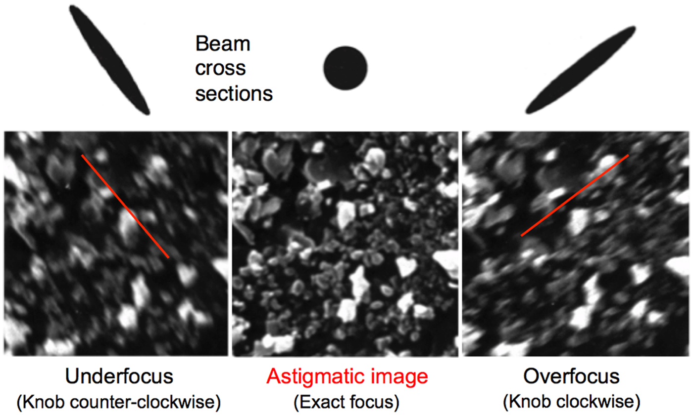
Figure 1: Through-focus images showing the stretching of the beam in orthogonal directions as the objective lens is first under-focused, brought to exact focus, and then over-focused. The out-of-focus images of particles are aligned with the shape of the elongated electron beam. At exact focus the image of random particles appears to be acceptable, but it is not. Image width = 12 μm.
To correct for astigmatism, the operator should find these steps helpful: (1) set the magnification to a high value such that the astigmatism can be detected, typically a step or two higher than that planned for image acquisition; (2) switch to rapid scan with a reduced raster; (3) set the objective lens at the best focus (exact focus) as shown in Figure 1; (4) sharpen the image with the x-stigmator control; (5) re-focus the image with the objective lens control; (6) sharpen the image with the y-stigmator; (7) re-focus the image; and (8) repeat steps 4 through 7 until the image cannot be further improved. Figure 2 shows the effect of removing astigmatism from the image: the image shows finer details because the probe size is smaller. Once the focus and stigmation are set at high magnification, these settings will be valid at all lower magnifications.
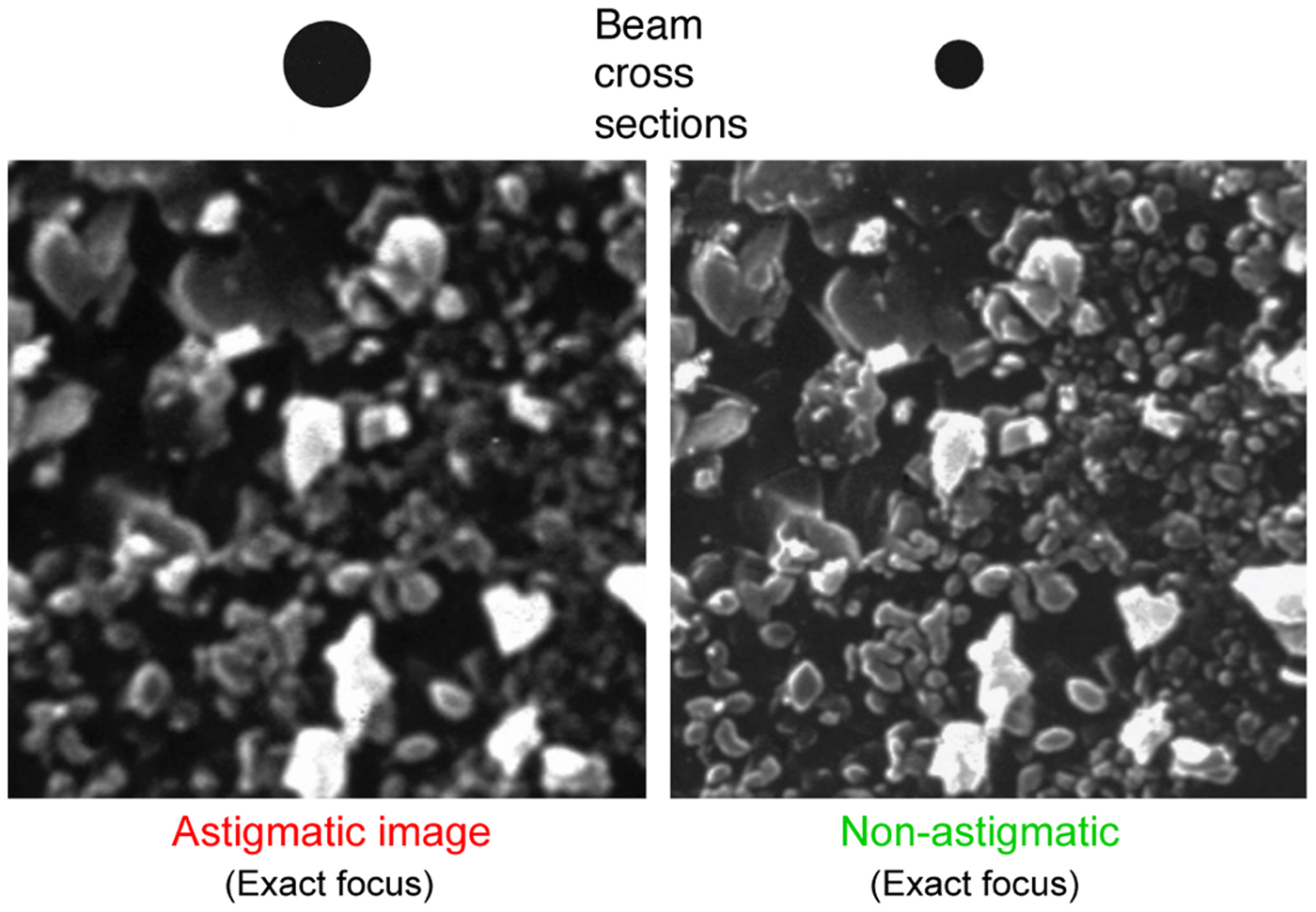
Figure 2: Images before and after astigmatism correction. At exact focus the astigmatic electron probe is larger than after correction when the contribution to the probe size attributable to astigmatism is eliminated. Image width = 10 μm.
If the image is noisy or of low contrast, not enough electron probe current was available in the specimen to produce a smooth, noise-free image. To mitigate noise in recorded images, the dwell time of the beam on each pixel could be increased, lengthening the image recording time. Another way to provide more current in the electron probe is to weaken the condenser lens a bit, which will also increase the probe size. But for low and medium magnifications, the larger current and resulting greater contrast will outweigh the increase in electron probe size (for probe sizes < 2 pixels at the specimen). These are changes to operating conditions that SEM operators might make multiple times in a single session if both low- and high-magnification images are required. With a field-emission electron source such situations are less likely because the electron probe typically will have a large current even at small probe sizes.
Incomplete astigmatism correction can be caused by the following: stigmating at the same magnification used for image acquisition, stigmating on non-random specimen details, and just using the focus and stigmator controls to sharpen the image without a strategy [Reference Goldstein1].


