


1. Introduction
Solute transport and chemical reactions in channel flows are of great interest in numerous engineering applications and natural processes, including microfluidics, biomedical devices and fractured rock hydrogeology (Kotomin & Kuzovkov Reference Kotomin and Kuzovkov1996; Dijk & Berkowitz Reference Dijk and Berkowitz1998; Detwiler, Rajaram & Glass Reference Detwiler, Rajaram and Glass2000; Losey et al. Reference Losey, Jackman, Firebaugh, Schmidt and Jensen2002; deMello Reference deMello2006; Meakin & Tartakovsky Reference Meakin and Tartakovsky2009; Kwon et al. Reference Kwon, Liebenberg, Jacobi and King2019; Lee & Kang Reference Lee and Kang2020; Yoon & Kang Reference Yoon and Kang2021). The reactive displacement of two miscible fluids in channel flows is a fundamental process that determines, for example, the performance of microfluidics devices and the remediation of contaminated fractured rock aquifers. In many of these applications, predicting the spatio-temporal evolution of chemical reactivity is critical. Here, we demonstrate that such prediction is possible through the concept of optimal fluid stretching, a concept that we propose in this study.
In a channel system where a solute  $A$ displaces another one $B$, the mixing front between $A$ and $B$ acts as a hot spot of reaction as mixing induces chemical disequilibrium by bringing together the reactants (Rolle & Le Borgne Reference Rolle and Le Borgne2019). If $A$ and $B$ are initially segregated, the reactive mixing front features strong chemical gradients, and the reaction process is mixing-limited at early times, which means that the time scale of mixing determines the overall reactivity. Therefore, in the mixing-limited pre-asymptotic regimes, the reaction rates predicted by models based on the well-mixed condition and (constant) hydrodynamic dispersion often lead to overestimation of the reaction process (Raje & Kapoor Reference Raje and Kapoor2000; Gramling, Harvey & Meigs Reference Gramling, Harvey and Meigs2002; Knutson, Valocchi & Werth Reference Knutson, Valocchi and Werth2007; Kang et al. Reference Kang, Bresciani, An and Lee2019; Lee et al. Reference Lee, Bresciani, An, Wallis, Post, Lee and Kang2020).
Understanding mixing and reaction processes in pre-asymptotic regimes is critical in many applications, but we still lack the mechanistic understanding of such processes. For example, in order to assess the efficiency of remediation strategies based on the mixing of contaminated groundwater with an injected reactant (Zavala-Sanchez, Dentz & Sanchez-Vila Reference Zavala-Sanchez, Dentz and Sanchez-Vila2009; Neupauer, Meiss & Mays Reference Neupauer, Meiss and Mays2014) and to optimize microfluidic mixers (Verguet et al. Reference Verguet, Duan, Liau, Berk, Cate, Majumdar and Szeri2010; Sivashankar et al. Reference Sivashankar, Agambayev, Mashraei, Li, Thoroddsen and Salama2016; Lee & Kang Reference Lee and Kang2020), the pre-asymptotic mixing mechanism should be quantified. In pre-asymptotic regimes, the classic Taylor–Aris approach based on effective dispersion cannot be applied because the solute has not yet sampled the full velocity spectrum across the channel cross-section. Therefore, chemical reactivity is not homogeneous over the channel cross-section, and local mixing processes such as fluid stretching determine the spatially non-homogeneous distribution of reactivity. Perez, Hidalgo & Dentz (Reference Perez, Hidalgo and Dentz2019b) recently investigated the global mixing and reaction behaviours (total mass product) and related them to an effective dispersion measure in channel flows. However, the local reaction behaviours, such as the temporal evolution of reaction locations in channel flows and its relation to local fluid deformation, are not yet clear.
Fluid stretching plays a critical role in enhancing mixing and reaction (Ottino, Ranz & Macosko Reference Ottino, Ranz and Macosko1979; Rhines & Young Reference Rhines and Young1983; Ottino Reference Ottino1989; Zoltan & Emilio Reference Zoltan and Emilio2009; Meunier & Villermaux Reference Meunier and Villermaux2010; Le Borgne, Dentz & Villermaux Reference Le Borgne, Dentz and Villermaux2013; Engdahl, Benson & Bolster Reference Engdahl, Benson and Bolster2014; Rolle & Le Borgne Reference Rolle and Le Borgne2019). In channel flows, shear flow by strong velocity gradients near the channel walls induces fluid stretching that leads to length elongation and width compression of a lamellar structure in the reaction front (de Anna et al. Reference de Anna, Jimenez-Martinez, Tabuteau, Turuban, Le Borgne, Derrien and Méheust2013; Bandopadhyay et al. Reference Bandopadhyay, Le Borgne, Méheust and Dentz2017; Souzy et al. Reference Souzy, Zaier, Lhuissier, Le Borgne and Metzger2018), meaning that the area of reactive mixing will be broadened and the reactants will be brought closer. Hence, fluid stretching promotes mixing and enhances reaction rates. Interestingly, two recent experimental studies have reported that there are optimal ranges of fluid stretching for maximum reactivity if the reaction systems are with an excitation threshold such as the Belousov–Zhabotinsky reaction (Nevins & Kelley Reference Nevins and Kelley2016; Wang et al. Reference Wang, Tithof, Nevins, Colón and Kelley2017). The authors found reaction blowout at high stretching rates, and this blowout is explained qualitatively by the dilution of the reactant due to the fluid stretching. However, the quantitative link between fluid stretching and mixing-limited reactions and the underlying mechanisms behind the optimal stretching are still elusive. If such a link can be established, one can envision predicting reactive transport from flow properties.
Many studies in recent years have investigated the relationship between fluid stretching and mixing-limited reaction processes. For instance, the Okubo–Weiss parameter (De Barros et al. Reference De Barros, Dentz, Koch and Nowak2012) and the trace of the local strain matrix squared (Aquino & Bolster Reference Aquino and Bolster2017) have been linked to the rate of evolution of the dilution index over time, demonstrating a correlation between the global mixing rate and fluid stretching. In Darcy-scale porous medium flows, Le Borgne, Dentz & Villermaux (Reference Le Borgne, Dentz and Villermaux2015) established a theory that predicts mixing from the concept of stretched lamellae. Engdahl et al. (Reference Engdahl, Benson and Bolster2014) and Wright, Richter & Bolster (Reference Wright, Richter and Bolster2017) also demonstrated a significant link between local high-reactivity and regions identified by multiple metrics of the fluid stretching, such as the Okubo–Weiss parameter, the largest eigenvalue of the Cauchy–Green strain tensor and finite-time Lyapunov exponents. Although these studies report correlations between the fluid stretching and reaction processes, underlying mechanisms by which the fluid stretching determines the spatially non-homogeneous reactivity in channel flows have not been elucidated.
In this study, we investigate the relationship between the fluid stretching and the mixing-limited reaction process in channel flows in pre-asymptotic regimes by combining numerical simulations using a Lagrangian reactive particle tracking algorithm (Perez, Hidalgo & Dentz Reference Perez, Hidalgo and Dentz2019a) and an analysis based on the diffusive strip method (Duplat & Villermaux Reference Duplat and Villermaux2008; Meunier & Villermaux Reference Meunier and Villermaux2010; Le Borgne et al. Reference Le Borgne, Dentz and Villermaux2013, Reference Le Borgne, Dentz and Villermaux2015; Perez et al. Reference Perez, Hidalgo and Dentz2019b). Especially, we aim to address the following open research questions: (a) What are the underlying mechanisms by which fluid stretching determines the spatial distribution of reactivity? (b) Is there an optimal stretching for inducing high reactivity and, if so, what causes the optimality? (c) Can we predict the spatial distribution of reactivity from stretching information alone? (d) How does the channel wall roughness affect the stretching–reactivity relationship?
This paper is structured as follows. In § 2, we present the method for obtaining channel flow fields and the reactive particle tracking algorithm for solving advection–diffusion–reaction equations. In § 3, we propose a new measure that quantifies fluid stretching using the concept of an effective time period. In § 4, we derive analytical solutions for the spatial distribution of reaction locations. In § 5, we present numerical simulation results, elucidate key mechanisms that determine a mixing-limited reaction and establish the quantitative link between fluid stretching and reactivity distributions. Finally, we discuss the effects of channel roughness on the stretching–reactivity relationship. Conclusions are presented in § 6.
2. Fluid flow and reactive transport in channel flows
2.1. Channel geometries and fluid flow
We consider both straight and rough channel flows in this study. The flow field in a straight channel is described by the parabolic velocity profile across the channel width as  $u(y) = u_0(1-y^2/a^2)$ for $-a \le y \le a$, where $u_0$ is the maximum velocity at the channel centre, and $a$ is half the channel width. In many natural and engineering applications, rough channel flows are common. We consider self-affine rough walls, as rough surfaces in nature are often found to be statistically self-affine (Mandelbrot Reference Mandelbrot1983; Kertesz, Horvath & Weber Reference Kertesz, Horvath and Weber1993; Ponson, Bonamy & Bouchaud Reference Ponson, Bonamy and Bouchaud2006; Ghanbarian, Perfect & Liu Reference Ghanbarian, Perfect and Liu2019). Self-affine surfaces are scale invariant in that the standard deviation of the height difference ${\rm \Delta} z$ between two points separated by lateral distance ${\rm \Delta} x$ can be expressed as $\sigma _{{\rm \Delta} z}({\rm \Delta} x) = \lambda ^{-H}\sigma _{{\rm \Delta} z}(\lambda {\rm \Delta} x)$, where $H$ is the Hurst exponent that characterizes the surface roughness (Drazer et al. Reference Drazer, Auradou, Koplik and Hulin2004; Liu et al. Reference Liu, Bodvarsson, Lu and Molz2004). We investigate the roughness effects by varying the Hurst exponent ( $H$) in the range of $0.7$– $0.9$, which covers the observable values in nature (Bouchaud, Lapasset & Planès Reference Bouchaud, Lapasset and Planès1990; Berkowitz Reference Berkowitz2002; Drazer et al. Reference Drazer, Auradou, Koplik and Hulin2004). We use the successive random addition algorithm (Voss Reference Voss1988; Liu et al. Reference Liu, Bodvarsson, Lu and Molz2004) to generate rough surfaces of $10$ cm length. The generated rough surfaces are duplicated and detached to have a constant channel width (aperture) of $b=1$ mm, where $b = 2a$.
We compute the fluid flow through the channels by solving the Navier–Stokes equations, using the finite volume method (OpenFOAM 2011), for steady-state incompressible laminar flow:
 \begin{gather} \boldsymbol{\nabla}\boldsymbol{\cdot}\boldsymbol{u}=0, \end{gather}
 \begin{gather}\boldsymbol{u}\boldsymbol{\cdot}\boldsymbol{\nabla} \boldsymbol{u}={-}\frac{1}{\rho}\boldsymbol{\nabla} p + \nu \nabla^2\boldsymbol{u}, \end{gather}
where  $\boldsymbol {u}$ is the pore-scale fluid velocity, $p$ is the fluid pressure and $\nu$ is the kinematic viscosity of the fluid. No-slip boundary conditions are applied at the channel walls. A constant flux boundary condition is imposed on the left boundary of the channels, and a zero-pressure-gradient boundary condition is imposed on the right boundary. The Reynolds number, defined as $Re={\bar {u}b}/{\nu }$, is set to one. Here, $\bar {u}$ denotes the mean flow velocity which is $0.01$ m s $^{-1}$ in this study. We discretize the fracture with a resolution of $0.01$ mm, yielding
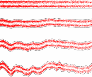
  $10\,000\times 100$ grid cells within the channel domain. Figure 1 shows velocity fields and initial reactant distributions for channels with different levels of roughness.

Figure 1. Channel geometries and initial distributions of  $A$ (red) and $B$ (black) reactants with the initial strip width of $w_0 = 5$ mm. Colour map indicates the normalized velocity magnitude.
2.2. Random walk based reactive particle transport
We consider an instantaneous irreversible bimolecular reaction
 \begin{equation} A + B \xrightarrow{k} C, \end{equation}
where  $k$ denotes the reaction rate coefficient. This elementary reaction can add up to describe complex reactions because complex reactions can be described by multiple elementary reaction steps (Gillespie Reference Gillespie2000). The transport of the reactant and product concentrations, $c_A$, $c_B$ and $c_C$ are described by the following advection–diffusion–reaction equations:
 \begin{gather} \frac{{\partial} c_A(\boldsymbol{x},t)}{{\partial} t} +\boldsymbol{\nabla}\boldsymbol{\cdot} \left( \boldsymbol{u}(\boldsymbol{x})c_A(\boldsymbol{x},t) \right) - D \nabla^2 c_A{(\boldsymbol{x},t)}={-}r(\boldsymbol{x},t), \end{gather}
 \begin{gather}\frac{{\partial} c_B{(\boldsymbol{x},t)}}{{\partial} t} +\boldsymbol{\nabla}\boldsymbol{\cdot} \left( \boldsymbol{u}(\boldsymbol{x})c_B(\boldsymbol{x},t) \right) - D \nabla^2 c_B{(\boldsymbol{x},t)}={-}r(\boldsymbol{x},t), \end{gather}
 \begin{gather}\frac{{\partial} c_C{(\boldsymbol{x},t)}}{{\partial} t} +\boldsymbol{\nabla}\boldsymbol{\cdot} \left(\boldsymbol{u}(\boldsymbol{x})c_C(\boldsymbol{x},t) \right) - D \nabla^2 c_C{(\boldsymbol{x},t)}=r(\boldsymbol{x},t), \end{gather}
where  $D$ is the diffusion coefficients of the species, $u(\boldsymbol {x})$ is the velocity field and $r(\boldsymbol {x},t)$ is the reaction rate, defined as $r(\boldsymbol {x},t)=kc_A{(\boldsymbol {x},t)}c_B{(\boldsymbol {x},t)}$. This simple reaction rule can represent many elementary chemical reactions (Rosenblatt, Hlinka & Epstein Reference Rosenblatt, Hlinka and Epstein1955; Smith et al. Reference Smith, Smart, Hancock and Twigg1989; Raje & Kapoor Reference Raje and Kapoor2000; Gramling et al. Reference Gramling, Harvey and Meigs2002; Lee & Kang Reference Lee and Kang2020). The simple reaction law allows us to reduce the complexity and thereby enables us to establish the mechanistic understanding of the coupling between the hydrodynamics and effective reaction dynamics. In this study, we consider the following initial conditions:
 \begin{gather} c_A(\boldsymbol{x},0) = \left\{\begin{array}{@{}ll@{}} c_0, & -w_0 < x < 0,\ \forall y\\ 0, & \textrm{otherwise}, \end{array}\right. \end{gather}
 \begin{gather}c_B(\boldsymbol{x},0) = \left\{\begin{array}{@{}ll@{}} c_0, & 0 < x < w_0,\ \forall y\\ 0, & \textrm{otherwise}, \end{array}\right. \end{gather}
 \begin{gather}c_C(\boldsymbol{x},0) =0,\ \forall y. \end{gather}
At  $t=0$, the two species $A$ and $B$ are vertically segregated at $x=0$ and the strip width of each reactant is $w_0$ (see figure 1). As we will see in the following sections, the initial width plays a key role in determining the optimal fluid stretching regime for enhanced reactivity.
We conduct numerical experiments using a random walk based reactive particle transport (RWPT) method (Perez et al. Reference Perez, Hidalgo and Dentz2019a). We briefly describe the method here. The equivalence between this RWPT method and the Eulerian reactive transport formulation (2.4) and its validation and application can be found in Perez et al. (Reference Perez, Hidalgo and Dentz2019a, Reference Perez, Hidalgo and Dentz). The simulation of reactive particle transport is based on the combination of a random walk method and a probabilistic rule for the reaction. The equation that governs the advective–diffusive motion of particles of the  $A$,
$A$,  $B$ and $C$ species is the following Langevin equation (Risken Reference Risken1996). The discretized Langevin equation is
 \begin{equation} \boldsymbol{x} \left( t + {\rm \Delta} t \right)=\boldsymbol{x}(t) + \boldsymbol{u}\left[ \boldsymbol{x}(t)\right]{\rm \Delta}{t} + \sqrt{2D{\rm \Delta} t}\boldsymbol{\eta}(t), \end{equation}
where  $\boldsymbol {x}(t)$ is the trajectory of a particle; $\boldsymbol {\eta }(t)$ are independent identically distributed Gaussian random variables characterized by zero mean and unit variance. The advective particle motion, $\boldsymbol {x} ( t + {\rm \Delta} t )=\boldsymbol {x}(t) + \boldsymbol {u}[ \boldsymbol {x}(t)]{\rm \Delta} {t}$, is simulated using a streamline based particle tracking algorithm (Bijeljic, Mostaghimi & Blunt Reference Bijeljic, Mostaghimi and Blunt2011; Mostaghimi, Bijeljic & Blunt Reference Mostaghimi, Bijeljic and Blunt2012). The Lagrangian approach to advection and diffusion is free of numerical dispersion and can accurately simulate particle transport even in high Péclet regimes.
At each time step, the position of each particle is recorded, and the distances between  $A$ and $B$ particles are calculated for the reaction step. We describe the point of view of a $B$ particle; that of an $A$ particle is analogous. The survival probability $P_s[\boldsymbol {x}(t)]$ of a $B$ particle in the time interval $[t, t+{\rm \Delta} t]$ depends on the number of $A$ particles, $N_A[\boldsymbol {x}(t)]$, within a well-mixed volume ${\rm \Delta} V$ centred at the position $\boldsymbol {x}(t)$ of a $B$ particle as (Perez et al. Reference Perez, Hidalgo and Dentz2019a)
 \begin{equation} P_s[\boldsymbol{x}(t)]=\exp [{-}p_r({\rm \Delta} t)N_A [\boldsymbol{x}(t)]], \end{equation}
where  $p_r({\rm \Delta} t)=k{\rm \Delta} t / (N_0{\rm \Delta} V)$ is the probability of a single reaction event, and $N_0$ is the total number of particles. The local reaction volume is ${\rm \Delta} V = {\rm \pi}r^2$, where the reaction radius is given as $r=\sqrt {4D{\rm \Delta} t}$ (Perez et al. Reference Perez, Hidalgo and Dentz2019a). The occurrence of a reaction event is determined through a Bernoulli trial based on the survival probability (2.7). If the reaction occurs, the $B$ particle and the closest $A$ particle are removed and a particle $C$ is placed at the middle point of the $A$ and $B$ particle locations. Since we consider an instantaneous reaction, the reaction probability $p_r$ in (2.7) is one. We inject $10^5$ particles for each species, and we vary the Péclet number, defined as $Pe={\bar {u}b}/{2D}$, to investigate the diffusion effects on mixing and reaction. To focus on diffusion effects, we fix $Re$ and vary $Pe$ by varying $D$. We consider four different $Pe$ regimes: $Pe=[10^2, 10^3, 10^4, 10^5]$.
3. Measures of fluid stretching
A key objective of this study is to elucidate the relation between the fluid stretching and reaction dynamics in channel flows. To investigate the stretching effects on mixing-limited reactive transport, we first need to define a measure that quantifies the degree of fluid stretching that controls mixing and reaction. We propose a Lagrangian way of quantifying the effective degree of fluid stretching, which honours the stretching history by adopting the concept of an effective time period.
Under a diffusion-limited condition, reactive particles tend to follow the streamlines and the advective stretching will play a dominant role in causing reactions. This means that we may need to honour the stretching history in quantifying the degree of fluid stretching that is required to induce reactions. In this context, we propose a Lagrangian stretching measure estimated from the right Cauchy–Green tensor with an effective time period where the effective time period is determined by the travel time for an infinitesimal fluid parcel of interest to arrive at the location of reaction from the initial location.
For comparison purpose, we also use the conventional Eulerian measure of fluid stretching that is based on the strain-rate tensor (De Barros et al. Reference De Barros, Dentz, Koch and Nowak2012; Engdahl et al. Reference Engdahl, Benson and Bolster2014; Aquino & Bolster Reference Aquino and Bolster2017). Because the strain-rate tensor is obtained from an instantaneous velocity field, the Eulerian measure quantifies the instantaneous strength of fluid stretching. This implies that in the Eulerian measure, the characteristic time for estimating stretching is fixed. We define both the Eulerian (instantaneous) and Lagrangian (history-honouring) measures of fluid stretching in the following subsections.
3.1. Eulerian measure of fluid stretching
The instantaneous stretching measure is based on the velocity gradient tensor defined as
 \begin{align} \boldsymbol{\epsilon} &= \boldsymbol{\nabla} \boldsymbol{u(x)} \nonumber\\ &= \left[\begin{array}{cc} \dfrac{{\partial} u}{{\partial} x} & \dfrac{{\partial} u}{{\partial} y} \\ \dfrac{{\partial} v}{{\partial} x} & \dfrac{{\partial} v}{{\partial} y} \end{array}\right]. \end{align}
The fluid stretching is quantified by the largest eigenvalue of the symmetric part of  $\boldsymbol {\epsilon }$ as
 \begin{equation} S_E =
\max[ \text{eig} [\tfrac{1}{2}(
\boldsymbol{\epsilon}+\boldsymbol{\epsilon}^* )
] ],
\end{equation}
\begin{equation} S_E =
\max[ \text{eig} [\tfrac{1}{2}(
\boldsymbol{\epsilon}+\boldsymbol{\epsilon}^* )
] ],
\end{equation}
where  $[\cdot ]^*$ denotes a matrix transpose. $S_E$ quantifies the instantaneous strength of stretching and shear deformation (Lapeyre, Klein & Hua Reference Lapeyre, Klein and Hua1999; De Barros et al. Reference De Barros, Dentz, Koch and Nowak2012).
In straight channels, the flow velocity is aligned with the channel and depends only on the position along the channel cross-section. Due to this feature, the velocity gradient tensor in a straight channel is
 \begin{equation}
\boldsymbol{\epsilon}= \left[\begin{array}{@{}cc@{}} 0 &
\alpha(y) \\ 0 & 0 \end{array}\right],
\end{equation}
\begin{equation}
\boldsymbol{\epsilon}= \left[\begin{array}{@{}cc@{}} 0 &
\alpha(y) \\ 0 & 0 \end{array}\right],
\end{equation}
where the shear rate,  $\alpha (y) = { {\partial } u}/{ {\partial } y}$, is given by
 \begin{equation} \alpha(y) ={-}2u_0y/a^2. \end{equation}
Thus, we obtain the Eulerian stretching measure as
 \begin{equation} S_E(\boldsymbol{x})=\frac{u_0|y|}{a^2}. \end{equation}
Note that this stretching measure is independent of  $x$ and only a function of $y$ in a straight channel, that is $S_E(\boldsymbol {x})=S_E(y)$. Figure 2(a) shows the Eulerian stretching map in the straight channel that we study. The Eulerian stretching is zero at the channel centre because the velocity gradient is zero at the channel centre, and increases linearly towards the channel wall.

Figure 2. (a) Eulerian stretching map,  $S_E(\boldsymbol {x})$ (3.5). (b) Lagrangian stretching map, $S_L(\boldsymbol {x})$ (3.11). (c) Analytical reactivity map for plug flow. (d) Analytical reactivity map for Poiseuille flow. (e) Reaction locations simulated by the RWPT method. The analytical reactivity maps and the numerical results are obtained for $Pe = 10^5$ and $w_0=5$ mm. The dashed lines are the characteristic depletion location, $x_R(y)$ (see § 5.2).
3.2. Lagrangian measure of fluid stretching
By definition, stretching measures quantify the strength of fluid stretching imposed on an elementary fluid volume over a certain characteristic time. Most studies fix the characteristic time when calculating stretching measures. For example, the Eulerian stretching measure based on the strain-rate tensor can be viewed as the rate of fluid stretching over unit time (De Barros et al. Reference De Barros, Dentz, Koch and Nowak2012; Engdahl et al. Reference Engdahl, Benson and Bolster2014; Aquino & Bolster Reference Aquino and Bolster2017). Also, the Lagrangian measures based on Cauchy–Green tensor is defined with a fixed time duration when calculating the deformation–gradient tensor (Voth, Haller & Gollub Reference Voth, Haller and Gollub2002; Arratia & Gollub Reference Arratia and Gollub2006; Engdahl et al. Reference Engdahl, Benson and Bolster2014; Nevins & Kelley Reference Nevins and Kelley2016; Wang et al. Reference Wang, Tithof, Nevins, Colón and Kelley2017).
However, fixing the characteristic time can lead to an ineffective quantification of fluid stretching when it comes to relating the stretching to reactions. Reactions depend on the processes that bring reacting species into contact, which are essentially fluid stretching and diffusion. In high  $Pe$ conditions, the chemical reactants are less likely to escape from the streamlines that they were initially in due to low diffusivity. This implies that the reactants retain the memory of the advective stretching they have gone through until they react, and the stretching history should be honoured in order to quantify the degree of fluid stretching required to induce the contact. Therefore, we propose a measure of fluid stretching using the concept of an effective time period in order to capture the effective degree of fluid stretching.
The proposed stretching measure is similar to the conventional Lagrangian stretching measure based on the Cauchy–Green tensor (Voth et al. Reference Voth, Haller and Gollub2002). The only difference is the manner of defining the time duration,  $T$, over which the Cauchy–Green tensor is computed. Given a velocity field $\boldsymbol {u(x)}$, we compute the flow map
 \begin{equation} \boldsymbol{F}(\boldsymbol{x})= \boldsymbol{x} + \int_{0}^{T} \boldsymbol{u}[\boldsymbol{x}(t)]\, \textrm{d} t, \end{equation}
where the effective time period  $T$ is determined such that a fluid element at $\boldsymbol {x}$ travels back to the initial location of the reaction front ( $x=0$) after backward time $T$ (i.e. $T<0$). Note that, given a velocity field $\boldsymbol {u(x)}$, $T$ is a function of $\boldsymbol {x}$ and defined in backward time ( $T<0$), which implies that we quantify the stretching imposed by advection during the prior time period $T$.
$T$.
The right Cauchy–Green strain tensor is then computed as
 \begin{equation} \boldsymbol{C}(\boldsymbol{x})=\left[ \boldsymbol{\nabla} \boldsymbol{F}(\boldsymbol{x}) \right]^* \left[ \boldsymbol{\nabla} \boldsymbol{F}(\boldsymbol{x}) \right],\end{equation}
where the deformation–gradient tensor  $\boldsymbol {\nabla } \boldsymbol {F}(\boldsymbol {x})$ is the gradient of the flow map with respect to $\boldsymbol {x}$. The maximum fluid stretching imposed by the effective time period can be estimated by the square root of the maximum eigenvalue of $\boldsymbol {C}(\boldsymbol {x})$ as
 \begin{equation} S_L(\boldsymbol{x}) = \sqrt{\max[\text{eig} [ \boldsymbol{C}(\boldsymbol{x})]]}. \end{equation}
Here,  $S_L(x)$ is the Lagrangian measure of fluid stretching that honours the history of fluid stretching. The well-known finite-time Lyapunov exponent is given by the logarithm of $S_L$ normalized by $T$ (
$T$ ( $\text {log}(S_L)/T$).
In straight channels, due to the geometric simplicity, we can compute the flow map explicitly as  $\boldsymbol {F}(\boldsymbol {x})= [x + u(y)\,T, y]^*$, where the effective time period for a spatial location $\boldsymbol {x}$ is $T=-x/u(y)$. Thus, the deformation–gradient tensor can be computed as
 \begin{equation}
\boldsymbol{\nabla} \boldsymbol{F}(\boldsymbol{x})=
\left[\begin{array}{@{}cc@{}} 1 & \dfrac{2xy}{a^2-y^2} \\
0 & 1
\end{array}\right].
\end{equation}
\begin{equation}
\boldsymbol{\nabla} \boldsymbol{F}(\boldsymbol{x})=
\left[\begin{array}{@{}cc@{}} 1 & \dfrac{2xy}{a^2-y^2} \\
0 & 1
\end{array}\right].
\end{equation}Then, the right Cauchy–Green strain tensor can be written as
 \begin{equation}
\boldsymbol{C}(\boldsymbol{x}) = \left[\begin{array}{@{}cc@{}} 1
& \dfrac{2xy}{a^2-y^2} \\
\dfrac{2xy}{a^2-y^2} & \left(
\dfrac{2xy}{a^2-y^2} \right)^2+1
\end{array}\right].
\end{equation}
\begin{equation}
\boldsymbol{C}(\boldsymbol{x}) = \left[\begin{array}{@{}cc@{}} 1
& \dfrac{2xy}{a^2-y^2} \\
\dfrac{2xy}{a^2-y^2} & \left(
\dfrac{2xy}{a^2-y^2} \right)^2+1
\end{array}\right].
\end{equation}Thus, we obtain for the Lagrangian stretching measure
 \begin{equation} S_L(\boldsymbol{x}) = \sqrt{ 1+2\left(\frac{xy}{a^2-y^2} \right)^2 +4 \sqrt{\left(\frac{xy}{a^2-y^2} \right)^4+\left(\frac{xy}{a^2-y^2} \right)^2} }. \end{equation}
Appendix A provides in detail the derivation from (3.9) to (3.11). Figure 2(b) shows the Lagrangian stretching map in the straight channel that we study. Like the Eulerian stretching, the Lagrangian stretching is zero at the channel centre. At  $x=0$, the Lagrangian stretching is zero across the channel width because the effective time period $T$ is zero. The stretching increases on moving downstream, and the increase is faster as it is closer to the channel wall. This is because the velocity gradient increases towards the channel wall, and $T$ increases with $x$.
$x$.
In rough channel flows, the flow map  $\boldsymbol {F}(\boldsymbol {x})$ cannot be analytically computed, and we use a streamline tracing algorithm that honours no-slip boundary conditions (Nunes, Bijeljic & Blunt Reference Nunes, Bijeljic and Blunt2015) to numerically compute $\boldsymbol {F}(\boldsymbol {x})$. The backward-time tracing can be straightforwardly conducted using the negative velocity field, $-\boldsymbol {u(x)}$, in the forward-time algorithm. Once $\boldsymbol {F}(\boldsymbol {x})$ is numerically calculated, we use (3.7) and (3.8) to compute $\boldsymbol {C}(\boldsymbol {x})$ and $S_L(\boldsymbol {x})$.
4. Reactivity map
The Eulerian and Lagrangian stretching measures (3.2) and (3.8) define stretching maps, which quantifies the spatial distribution of fluid stretching. To investigate the link between fluid stretching and chemical reaction, we compare the stretching maps to a reactivity map  $m(\boldsymbol {x})$, which is defined here as the total amount of $C$ produced at a location $\boldsymbol x$ over time,
 \begin{gather} \frac{\textrm{d} m(\boldsymbol{x},t)}{\textrm{d} t} = r(\boldsymbol{x},t). \end{gather}
 \begin{gather}m(\boldsymbol{x}) = \int r(\boldsymbol{x},t) \,\textrm{d} t. \end{gather}
Here,  $m(\boldsymbol {x})/\int m(\boldsymbol {x}) \,\textrm {d}\kern0.7pt\boldsymbol {x}$ can also be understood as a spatial probability density function (PDF) that shows the spatial distribution of reaction locations integrated over time. Here we consider a fluid–fluid reaction, in which all species are mobile. The analysis and mathematical framework are equally valid for a reaction, in which the product species $C$ is immobile. In this case, $m(\boldsymbol x,t)$ provides a spatial map of the reaction product that does not evolve in time. Therefore, the reactivity map also has direct implications for reactions that produce immobile reaction products. In the following sections, we determine the reactivity maps for straight and rough channels using the reactive particle tracking methodology of § 2.2. For the case of plug flow and Poiseuille flow in a straight channel, the reactivity map can be determined analytically as follows.
4.1. Analytical solution for plug flow in a straight channel
Let us consider first the reactivity map  $m(\boldsymbol {x})$ for a plug flow with constant flow velocity $u$. Advection–diffusion and reaction in plug flow through a straight channel is described by (2.4) for $u(\boldsymbol x) = u =$ constant. In this case the solution of the concentration of the reaction product $C$ is given by (Perez et al. Reference Perez, Hidalgo and Dentz2019b)
 \begin{equation} c_C(x,t) = \frac{c_0}{2} \left[\text{erfc}\left(\frac{x - ut}{\sqrt{4Dt}} \right) - \text{erfc}\left(\frac{x +w_0 - ut}{\sqrt{4Dt}} \right) \right] \end{equation}
for  $x \geq u t$, and
 \begin{equation} c_C(x,t) = \frac{c_0}{2} \left[\text{erfc}\left(\frac{x -w_0 - ut}{\sqrt{4Dt}} \right) - \text{erfc}\left(\frac{x - ut}{\sqrt{4Dt}} \right) \right] \end{equation}
for  $x < ut$.
Solving for the reactivity map (4.2) requires deriving an analytical expression for the reaction rate  $r({\boldsymbol x},t)$. To this end, we integrate (2.4c) from $ut - \epsilon$ to $ut + \epsilon$ with $\epsilon > 0$ in order to obtain
 \begin{equation} - D \left.\frac{\partial c(x,t)}{\partial x}\right|_{x = ut - \epsilon} + D \left.\frac{\partial c(x,t)}{\partial x}\right|_{x = ut + \epsilon} = \int_{ut -\epsilon}^{ut + \epsilon} {\textrm{d}\kern0.6pt x}\, r(x,t). \end{equation}
We used here the fact that the species concentration is continuous at the interface, while the derivative of (4.3) is discontinuous at  $x = ut$. It is given by
 \begin{equation} \left.\frac{\partial c(x,t)}{\partial x}\right|_{x = ut \pm \epsilon} ={\mp} c_0 \left[ \frac{\exp\left(- \dfrac{(\epsilon-w_0)^2}{4 D t} \right)}{\sqrt{4{\rm \pi} D t}} - \frac{\exp\left(- \dfrac{\epsilon^2}{4 D t} \right)}{\sqrt{4 {\rm \pi}D t}} \right]. \end{equation}
Inserting this expression into (4.4), we obtain
 \begin{equation} \lim_{\epsilon \to 0} \int_{ut -\epsilon}^{ut + \epsilon} {\textrm{d}\kern0.6pt x}\, r(x,t) = \frac{c_0}{\sqrt{{\rm \pi} D t}} \left[1 - \exp\left(- \frac{w_0^2}{4 D t} \right)\right]. \end{equation}
This implies that
 \begin{equation} r(x,t) = \frac{c_0 \sqrt{D}}{\sqrt{{\rm \pi} t}} \left[1 - \exp\left(- \frac{w_0^2}{4 D t} \right)\right] \delta(x - ut). \end{equation}
Inserting this expressing for  $r(x,t)$ into the right side of (4.1) and integrating over time gives $m(x,t) = m(x) H(u t - x)$, where we defined
 \begin{equation} m(x) = \frac{c_0\sqrt{D}}{\sqrt{{\rm \pi} x u}} \left[1 - \exp\left(- \frac{w_0^2 u }{4 D x} \right)\right]. \end{equation}
Figure 2(c) shows the reactivity map  $m(x)$ for $w_0=5$ mm and $Pe=10^5$. The Heaviside function $H(ut-x)$ expresses the fact that reaction can only happen behind the advancing interface for $x < ut$. Thus the map shown in figure 2(c) can be interpreted as the reactivity map after the interface sweeps the channel domain. For distances $x \ll w_0^2 u/D$, the reactivity decays with travel distance as $x^{-1/2}$. For large distances $x \gg w_0^2 u/D$ it decays as $x^{-3/2}$. This decay in reactivity is due to the fact that concentration gradients, which drive the reaction, attenuate due to diffusion.
4.2. Analytical solution for Poiseuille flow in a straight channel
We now consider Poiseuille flow in a straight channel. Advection–diffusion–reaction is described by (2.4), and Poiseuille flow through a straight channel is described by the parabolic velocity field,  $u(y) = u_0 (1 - {y^2}/{a^2} ).$ To analytically solve the advection–diffusion–reaction problem, we use the stretched lamella formulation (Meunier & Villermaux Reference Meunier and Villermaux2010; Le Borgne et al. Reference Le Borgne, Dentz and Villermaux2013), which quantifies mixing due to advective stretching of the substrate and diffusion across it. Thus, it is valid as long as transverse diffusion has not led to substantial mixing across the channel. When this occurs, the approximation of the interface as a stretched lamella breaks down, as we will see below.
The solution requires transforming the advection–diffusion reaction problem (2.4) from the fixed ( $x,y$) coordinate system into local coordinates that move and rotate with a material element that is initially aligned with the interface between the $A$ and $B$ species at $x=x_0$ and oriented perpendicular to the mean flow direction. By this transformation, (2.4c) can be recast as (Bandopadhyay et al. Reference Bandopadhyay, Le Borgne, Méheust and Dentz2017; Dentz et al. Reference Dentz, de Barros, Le Borgne and Lester2018; Perez et al. Reference Perez, Hidalgo and Dentz2019b)
 \begin{equation} \frac{{\partial} \hat{c}(\hat{x},t\,|\,y)}{{\partial} t}-\frac{1}{\lambda(t\,|\,y)} \frac{\textrm{d} \lambda(t\,|\,y)}{\textrm{d} t} \hat{x} \frac{{\partial} \hat{c}(\hat{x},t\,|\,y)}{{\partial} \hat{x}} - D \frac{{\partial}^2 \hat{c}(\hat{x},t\,|\,y)}{{\partial} \hat{x}^2}=\hat{r}(\hat{x},t\,|\,y), \end{equation}
where we omit the subscript  $C$ for brevity, and $\hat {x}$ is the coordinate perpendicular to the lamella. The relative elongation of the lamella centred at $[ u(y)t, \ y ]^*$ is $\lambda (t\,|\,y) = \sqrt {1 + \alpha (y)^2t^2}$, where the shear rate $\alpha (y)$ is given by (3.4). This equation can be transformed into a simple diffusion–reaction equation by the coordinate transformation
 \begin{gather} x'=\hat{x}\lambda(t|y), \end{gather}
 \begin{gather}\tau(t\,|\,y)=\int_0^t\textrm{d} t'\, D \lambda(t'\,|\,y)^2 = D[t+\alpha(y)^2t^3/3]. \end{gather}
Thus, we obtain the diffusion–reaction equation
 \begin{equation} \frac{{\partial} c'(x',\tau)}{{\partial} \tau} - \frac{{\partial}^2 c'(x',\tau)}{{\partial} {x'}^2} = \frac{r'(x',t)}{D\lambda(t)^2}, \end{equation}
where we omit the  $y$-dependence for brevity. From here on, the methodology is analogous to the one used in the previous section in order to derive an analytical expression for $r'(x',t)$ in the stretched coordinates attached to the lamella. Transformation back into the original coordinate system gives
 \begin{equation} r(\boldsymbol{x},t)= \frac{c_0}{\sqrt{{\rm \pi}\tau(x/u) }} \left[ 1-\exp \left( -\frac{w_0^2}{4\tau(x/u)} \right) \right] D\lambda(x/u)^2 \delta\left(x-u t\right). \end{equation}
For details, see Appendix B. Inserting expression (4.13) into (4.1) and integrating over time gives for the reactivity map  $m(\boldsymbol {x},t) = m(\boldsymbol {x}) H(u t-\boldsymbol {x})$, where $m(\boldsymbol {x})$ is defined by
 \begin{equation} m(\boldsymbol{x}) = \frac{c_0}{u\sqrt{{\rm \pi}\tau(x/u)}} \left[ 1-\exp \left( -\frac{w_0^2}{4\tau(x/u)} \right) \right] D\lambda(x/u)^2. \end{equation}
Figure 2(d) shows the map  $m(\boldsymbol {x})$ for $w_0=5$ mm and $Pe=10^5$. The Heaviside function $H[u(y)t-x]$ indicates that a reaction can only happen behind the advancing interface for $x < u(y)t$. Thus the map shown in figure 2(d) can be interpreted as the reactivity map at large $t$ after the interface sweep the channel domain. For, large distances such that $D \alpha ^2 (x/u)^3 \gg w_0^{2}$, reactivity decays as $x^{-5/2}$. The faster decay compared to the plug flow scenario is due to the fact that much of the reactant is consumed at short distances by the enhanced stretching, which leads to a faster decay. Note that the reactivity maps between plug flow and Poiseuille flow are dramatically different (figure 2c,d).
5. Results and discussion
In this section, we first analyse the spatial distributions of reaction locations in straight channel flows from stretching-dominated (high  $Pe$) to diffusion-dominated (low $Pe$) regimes (§ 5.1), elucidate how the fluid stretching determines the spatial distributions of reaction locations (§ 5.2) and identify optimal stretching regimes and extend the findings to rough channel flows (§ 5.3).
5.1. Spatial distribution of reaction locations
We solve the advection–diffusion–reaction equations (ADRE) in (2.4) using the RWPT method described in § 2.2. The strip widths of the solutes  $A$ and $B$ at $t=0$ are both $w_0=5$ mm. A great benefit of the Lagrangian approach for solving the ADRE is that the spatial locations of reaction occurrence can be obtained, as shown in figure 2(e), and compared with the analytical solution (figure 2d). This feature enables us to explicitly analyse the stretching–reactivity relation because we can sample the stretching values corresponding to the reaction locations from the stretching maps (e.g. figure 2a,b).
We first investigate high  $Pe$ regimes ( $Pe=[10^4, 10^5]$) to focus on stretching-controlled mixing regimes. For low $Pe$ regimes ( $Pe=[10^2, 10^3]$), the role of diffusion on mixing increases, and the combined effects of stretching and diffusion should be considered to understand mixing and reaction. Figure 3(a,c) shows the spatial distribution of reaction locations simulated by the RWPT method for $Pe=[10^4, 10^5]$ in the straight channel shown in figure 1. The channel centre ( $y=0$) has few reaction occurrences because shear rate, which determines fluid stretching, is zero at the channel centre. The active reaction zone is near walls at upstream locations and moves towards the channel centre on moving downstream.

Figure 3. (a) Empirical reactivity map where red dots are individual reaction locations, and (b) the empirical PDF of  $y$-coordinates of reaction locations (red solid lines) along with the black dashed lines showing the reactivity-weighted PDF of $y$-coordinates computed by (5.1) at $Pe=10^4$. (c) Empirical reactivity map showing reaction locations, and (d) the PDF of $y$-coordinates of reaction locations at $Pe=10^5$. The active reaction zones upstream are near the wall and move towards the channel centre on moving downstream. The analytical prediction (black dashed lines) accurately captures the simulation results (red solid lines).
The similar trend (the convergence of the active reaction zone towards the channel centre in the downstream direction) is also captured in the analytical reactivity map for Poiseuille flow (4.14). Figure 2(d,e) shows that the analytical reactivity map for  $Pe=10^5$ qualitatively matches with the spatial distribution of reaction locations simulated by the RWPT. To quantitatively compare the maps, we estimate the PDF of $y$-coordinates of reaction locations from the reactivity map as
 \begin{equation} P(y)=\frac{\displaystyle\int {\textrm{d}\kern0.6pt x}\, m(\boldsymbol{x})}{\displaystyle\int \textrm{d}\kern0.6pt\boldsymbol{x}\, m(\boldsymbol{x})}. \end{equation}
Figure 3(b,d) compares  $P(y)$ from the analytical solution, $P_{analy}(y)$, with $P(y)$ from the numerical simulation, $P_{sim}(y)$, at every $1$ cm interval; $P_{analy}(y)$ and $P_{sim}(y)$ show an excellent match across the channel domain, indicating that the analytical prediction accurately captures the location of high reactivity over the whole channel.
Fluid stretching is well known to increase mixing by increasing the interfacial area between reactants, thereby promoting the overall reaction. Thus, one may conjecture that the active reaction zone is always near walls where the degree of stretching is maximum. However, the active reaction zone is near walls only at upstream locations and moves away from the walls on moving downstream, as shown in figure 3. We hypothesize that the near-wall low reactivity in downstream regions is because the reactants near walls react and are consumed early, and no reactants are available near walls in downstream regions. In § 5.2, we confirm this hypothesis by analytically deriving the time scale required to deplete the reactants and elucidate the underlying mechanism inducing the evolution of the reactive zone locations.
Figure 4 shows the spatial distribution of reaction locations obtained from numerical simulations, and the comparison between  $P_{sim}(y)$ and $P_{analy}(y)$ for $Pe=[10^2, 10^3]$. Similar to the high $Pe$ cases, low reactivities at the channel centre throughout the channel length and at the near-wall locations in downstream regions are observed. However, the movement of the reactive zone towards the channel centre is only observed in upstream regions, whereas the analytical solution, $P_{analy}(y)$, predicts that the convergence behaviour continues throughout the channel length (figure 4(b,d), black dashed lines).

Figure 4. (a) Empirical reactivity map where red dots are individual reaction locations, and (b) the empirical PDF of  $y$-coordinates of reaction locations (red solid lines) along with the black dashed lines showing the reactivity-weighted PDF of $y$-coordinates computed by (5.1) at $Pe=10^2$. The active reaction zones are independent of $x$ after $x\approx 2$ cm. (c) Empirical reactivity map showing reaction locations, and (d) the PDF of $y$-coordinates of reaction locations at $Pe=10^3$. The active reaction zones are independent of $x$ after $x\approx 3$ cm. The analytical prediction (black dashed lines) captures the simulation results only near the injection location.
The analytical reactivity map (4.14) is derived assuming no transverse diffusion across lamellar structures. This means that the assumption will become no longer valid as the transverse diffusion effects on mixing increase, and the transverse diffusion effects will appear earlier for lower  $Pe$ conditions. This is why the analytical solution breaks down earlier for $Pe=10^2$ compared to $Pe=10^3$. For $Pe=10^2$, the analytical prediction does not match the simulation results before $1$ cm, indicating that the transverse diffusion plays a significant role before $x=1$ cm. When we subdivide the first $1$ cm channel segment, we can confirm that $P_{analy}(y)$ accurately captures $P_{sim}(y)$ up to $x\approx 8$ mm, as shown in figure 5. This confirms that the analytical solution is valid as long as transverse diffusion is limited. The mismatch near the wall in the $0$–
$0$– $2$ mm zone is due to the finite-size effects of the number of injected particles.

Figure 5. (a) Empirical reactivity map where red dots are individual reaction locations, and (b) the empirical PDF of  $y$-coordinates of reaction locations in the first $1$ cm channel segment at $Pe=10^2$. The analytical prediction (black dashed lines) captures the simulation results near the injection location.
5.2. Mechanisms and prediction of the locations of maximum reactivity
The convergence of high-reactivity zones from the channel walls towards the channel centre is due to the combined effects of stretching-enhanced reaction and the depletion of the reactants. This interplay creates the regions of maximum reaction discussed in the previous section. We illustrate this mechanism by considering the time scale required to deplete the reactant species that has the initial width of  $w_0$. In plug flow, the characteristic time for mass depletion is simply given by the diffusion time over $w_0$,
 \begin{equation} \tau_D=\frac{w_0^2}{2D}. \end{equation}
In the channel flow, the velocity gradient is stretching the strips. Stretching is stronger close to the wall because the shear rate increases linearly from channel centre to channel wall. The time evolution of strip width,  $w(t)$, is determined by stretching and diffusion, which can be expressed by the following balance equation (Villermaux Reference Villermaux2012; Dentz & de Barros Reference Dentz and de Barros2015):
 \begin{equation} \frac{1}{w(t)}\frac{\textrm{d} w(t)}{\textrm{d} t}={-}\gamma(t)+\frac{D}{w(t)^2}. \end{equation}
The stretching rate  $\gamma (t)$ is given by
 \begin{equation} \gamma(t) = \frac{1}{\ell(t)}\frac{\textrm{d}\ell(t)}{\textrm{d} t}, \end{equation}
where  $\ell (t)$ is the strip elongation. In the shear flow through the channel, it is
 \begin{equation} \ell(t) = \ell_0\sqrt{1 + \alpha(y)^2t^2}. \end{equation}
Thus, the stretching rate is
 \begin{equation} \gamma(t) = \frac{\alpha(y)^2t}{1+\alpha(y)^2t^2}. \end{equation}
From (5.3) and (5.6), we obtain the width evolution due to stretching only as  $w_s(t)=w_0/\sqrt {1+\alpha (y)^2t^2}$, by setting $D = 0$ in (5.3). The reaction depletes at $t = \tau _m$ when the width $w_s(\tau _m)$ is equal to the diffusive width $\sqrt {2D\tau _m}$ because the strip has been compressed sufficiently such that diffusion mixes the full strip width. This implies
 \begin{equation} 2D\tau_m=\frac{w_0^2}{1+\alpha(y)^2\tau_m^2}. \end{equation}
For large elongation (i.e.  $\alpha (y)^2\tau _m^2\gg 1$), the depletion time $\tau _m$ is
 \begin{equation} \tau_m(y)=\alpha(y)^{{-}2/3}\left( \frac{w_0^2}{2D}\right)^{1/3}=\alpha(y)^{{-}2/3}\tau_D^{1/3}. \end{equation}
The reaction location  $x_R(y)$ corresponding to the depletion time can be calculated by $x_R(y) = u(y) \tau _m(y)$. Figure 6 shows the reactivity map, $m(\boldsymbol {x})$, along with the characteristic depletion location (red dashed lines), $x_R(y)$, for $Pe=[10^2,10^3,10^4,10^5]$. Clearly, the depletion of the reactant species causes the reactive zone to move towards the channel centre on moving downstream. Also, the movement towards the centre is more rapid as $Pe$ decreases. This is because the reactants are more rapidly consumed by diffusion-induced mixing and reaction as implied by the factor $\tau _D^{1/3}$ in (5.8). Note that this derivation neglects diffusion transverse to lamellar structures, which can be important at later times. This is why the convergence of reaction locations towards the channel centre is faster in the analytical solution than what is obtained from direct numerical simulations in low $Pe$ regimes (figure 4b,d).

Figure 6. Reactivity maps (4.14) according to  $Pe$ in a straight channel flow. The dashed lines are the characteristic depletion location, $x_R(y)$. The active reaction zones upstream are near the wall and move towards the channel centre on moving downstream. (a) Pe = 102; (b) Pe = 103; (c) Pe = 104; (d) Pe = 105.
The reaction depletion near the channel walls emerges because the mass of reactants is limited. The importance of the mass limitation is highlighted by considering the effect of the initial strip width,  $w_0$. Figure 7 shows the reactivity map, $m(\boldsymbol {x})$, along with the characteristic depletion location, $x_R(y)$, for $Pe=10^5$ for different initial strip widths, $w_0$. As $w_0$ increases, that is, as the mass limitation is alleviated, the reactive zone stays near the wall for larger distances. This confirms that the competition between the enhanced mixing by fluid stretching and the mass limitation of the reactants underlies the movement of the high-reactivity zone towards the channel centre on moving downstream.

Figure 7. Reactivity maps (4.14) for the three different values of  $w_0$ in a straight channel flow. The dashed lines are the characteristic depletion location, $x_R(y)$. As the mass limitation is eased (as $L$ increases), the active reaction zone stays near the channel wall, where fluid stretching is stronger, for longer distances. (a) W 0 = 1 mm; (b) W 0 = 5 mm; (c) W 0 = 10 mm.
In summary, we have shown how the compound effects of fluid stretching, diffusion and mass limitation determine the local reactivity in straight channel flows. Especially for high  $Pe$ regimes ( $Pe\ge 10^4$), the role of fluid stretching on mixing is dominant over that of the diffusion effects for the whole channel domain. Consequently, the analytical reactivity map can predict where and how much reaction products are produced for the whole domain. This leads us to a hypothesis that, if stretching-induced mixing is dominant, characterizing the fluid stretching will be sufficient for predicting the distribution of reactivity. We investigate this hypothesis in the following subsection by analysing the stretching–reactivity relationship for the high $Pe$ regimes.
5.3. Stretching–reactivity relationship: optimal stretching and roughness effects
We combine the reactivity maps and the maps of Eulerian and Lagrangian stretching to establish stretching–reactivity relationship. While the Eulerian measure is independent of  $x$, the Lagrangian measure of fluid stretching is zero at the initial location of the reaction front ( $x=0$) and increases with $x$ (figure 2a,b). The increase depends on the shear rate, which is strongest at the wall and zero at the channel centre. For $Pe=[10^4, 10^5]$, we compute the reactivity-weighted PDF of both measures as
 \begin{gather} P(S_E) =\dfrac{\displaystyle\int \textrm{d} m \, m P(m,S_E)}{\displaystyle\int \textrm{d} S_E \displaystyle\int \textrm{d} m \, m P(m,S_E)}, \end{gather}
 \begin{gather}P(S_L) =\dfrac{\displaystyle\int \textrm{d} m \, m P(m,S_L)}{\displaystyle\int \textrm{d} S_L \displaystyle\int \textrm{d} m \, m P(m,S_L)}, \end{gather}
where the joint PDF  $P(m,S) = \int _\varOmega \textrm {d}\kern0.7pt \boldsymbol {x} \, \delta ( S-S(\boldsymbol {x}) ) \delta ( m-m(\boldsymbol {x}) ) / \int _\varOmega \textrm {d}\kern0.7pt\boldsymbol {x}$. Here, $\varOmega$ denotes the channel domain and $\delta (\cdot )$ is the Dirac delta function. Figure 8 shows $P_{analy}(S_E)$ and $P_{analy}(S_L)$ from the analytical solution along with the corresponding empirical PDFs, $P_{sim}(S_E)$ and $P_{sim}(S_L)$, of the stretching metrics sampled at reaction locations simulated by the RWPT method.

Figure 8. Empirical PDFs of Eulerian and Lagrangian stretching values sampled from reaction locations for (a)  $Pe=10^4$ and (b) $Pe=10^5$ for the straight channel. The black dashed lines are analytically computed reactivity-weighted PDFs of fluid stretching (5.9). The observed stretching–reactivity relations demonstrate that there exist optimal ranges of fluid stretching for high reactivity.
As can be expected from the good agreement between the analytical prediction and the numerical experiments in figure 3, the predicted and simulated stretching–reactivity relationships are in good agreement. It is noteworthy that the modes of  $P_{analy}(S_E)$ and $P_{analy}(S_L)$ are not located at the maximum value of stretching. One may expect the mode of the reactivity-weighted PDFs to be the maximum value of the support of the PDFs because larger fluid stretching leads to larger mixing. However, as discussed in §§ 5.1 and 5.2, this is not the case due to the mass limitation of the reactants. The competition between the enhanced mixing by fluid stretching and the mass depletion of the reactants results in the emergence of an optimal range of fluid stretching for high reactivity.
Now we extend our analysis to rough channels to check if the optimality of fluid stretching is maintained in more complex flow fields. Figure 9(a–d) shows the distribution of reaction locations simulated by the RWPT method and the empirical PDF of  $y$-coordinates sampled from the reaction locations for the case of $H=0.8$ and $Pe=[10^4, 10^5]$. The $y$-coordinate ranges from $-0.5$ mm at the bottom wall to $0.5$ mm at the upper wall. Similar to the straight channel case shown in figure 3, the evolution of the high-reactivity zone on moving downstream is observed. This implies that the competition between the enhanced mixing by fluid stretching and the mass depletion of the reactants also determines the location of high reactivity in rough channels.

Figure 9. (a) Empirical reactivity map where red dots are individual reaction locations, and (b) the empirical PDF of  $y$-coordinates of reaction locations (red solid lines) at $Pe=10^4$. The black dashed lines show the analytical prediction from the straight channel (the reactivity-weighted PDF of $y$-coordinates computed by (5.1)). (c) Empirical reactivity map showing reaction locations, and (d) the PDF of $y$-coordinates of reaction locations for $Pe=10^5$. (e) Eulerian stretching map. ( f) Lagrangian stretching map. The results are for $H=0.8$. The active reaction zones upstream are near the wall and move towards the channel centre on moving downstream.
We numerically compute the maps of Eulerian and Lagrangian stretching,  $S_E$ (3.2) and $S_L$ (3.8), respectively as shown in figure 9(e, f). The channel roughness increases the complexity of the stretching maps. We then calculate the empirical PDFs, $P_{sim}(S_E)$ and $P_{sim}(S_L)$, of the stretching metrics sampled at reaction locations simulated by the RWPT method in rough channel flows ( $H=0.8)$, as shown in figure 10. Black dashed lines show $P_{analy}(S_E)$ and $P_{analy}(S_L)$, which are computed from the analytical reactivity map of the straight channel (5.9).

Figure 10. Empirical PDFs of Eulerian and Lagrangian stretching values sampled from reaction locations for (a)  $Pe=10^4$ and (b) $Pe=10^5$. The dashed lines are the reactivity-weighted PDFs of fluid stretching, analytically computed from (5.9) for the straight channel. The vertical lines indicate the shortest ranges accounting for 70 % mass of the PDFs. The stretching–reactivity relations analytically predicted for the straight channels are maintained for the more complex flow fields in the rough channels.
The reactivity-weighted PDF of Eulerian stretching for the rough channel deviates significantly from that for the straight channel (figure 10). The Eulerian quantity of fluid stretching is computed using the spatial gradients of flow velocities, as in (3.2). Thus, the significant deviation is from the flow complexity induced by the channel roughness. In contrast to the Eulerian measure, the reactivity-weighted PDF of Lagrangian stretching for the straight channel agrees very well with that for the rough channel. This implies that the proposed Lagrangian stretching measure is the measure that accurately predicts the reaction locations by properly honouring the stretching history. In other words, this result indicates that honouring the stretching history with the concept of the effective time period is critical for properly quantifying the effective degree of fluid stretching that determines mixing-limited reactions. Furthermore, the reactivity-weighted PDFs of the Lagrangian stretching measure seem independent of channel roughness, and this implies that there may be optimal stretching ranges that are independent of channel roughness.
To confirm the importance of honouring the stretching history and the existence of a roughness-independent optimal stretching range, we quantitatively compare optimal stretching regimes of  $S_E$ and $S_L$ across the channel roughness. We estimate the shortest range of fluid stretching accounting for $70$ % mass of the PDFs, $P_{analy}(S_E)$ and $P_{analy}(S_L)$, as shown in figures 10 (line bars) and 11 (circle symbols with ranges). The $70$ % is chosen considering the fact that the mass of normal distribution within one standard deviation of the mean accounts for approximately $68$ %. We also estimate the range of fluid stretching corresponding to the same mass of the empirical PDFs, $P_{sim}(S_E)$ and $P_{sim}(S_L)$, computed for rough channels with $H=[0.7, 0.8, 0.9]$, and plot the middle points of the ranges as shown in figure 11 (dashed lines with triangle, cross and square symbols).

Figure 11. Estimated optimal stretching ranges as a function of channel length for  $S_E$ (a,b) and $S_L$ (c,d) at $Pe=[10^4, 10^5]$. The circles with ranges show optimal stretching ranges that are analytically obtained for the straight channels. Other lines with different symbols show optimal stretching values that are numerically obtained for three different channel roughness, $H=[0.7, 0.8, 0.9]$. The ranges of the Lagrangian stretching measure, $S_L$, obtained from the analytical solution for straight channels accurately capture the optimality in rough channel flows.
For the Lagrangian stretching measure,  $S_L$, the analytically computed ranges of optimal stretching for straight channels accurately capture the optimal stretching values across channel roughness (figure 11c,d). However, the Eulerian stretching measure, $S_E$, between the straight channel and rough channels shows significant differences (figure 11a,b). This result highlights that, although the channel roughness induces complex flow fields and thereby the complex distribution of fluid stretching, the Lagrangian stretching–reactivity relationship is rather consistent, and the optimality of fluid stretching for mixing and reaction is maintained across different levels of channel roughness.
6. Conclusions
Mixing-limited reactions in pre-asymptotic regimes are strongly determined by fluid stretching. In this study, we have established the quantitative link between fluid stretching and reactivity in channel flows, which enables the prediction of chemical reactivity from fluid stretching information only. We considered an instantaneous irreversible bimolecular reaction ( $A + B \rightarrow C$) in finite-length channels and simulated the advection–diffusion–reaction process using a RWPT method. The numerical simulations revealed the convergence of reaction locations towards the channel centre in the downstream direction and the optimal ranges of stretching for high reactivity.
We quantitively elucidated the origin of optimal stretching as the competition between stretching-induced mixing enhancement and mass limitation that is determined by the initial reactant strip width. To quantify the key mechanisms, we analytically derived the spatial distribution of reactivity in straight channels using a lamellar formulation. The analytical solution accurately captured results obtained from direct numerical simulations. We also proposed the Lagrangian measure of fluid stretching based on the concept of the effective time period and captured the consistent relation between fluid stretching and mixing-limited reaction. From the proposed definition of fluid stretching and the analytical derivation, we demonstrated the existence of optimal fluid stretching for high reactivity.
The optimality is not a straightforward result. Fluid stretching is well known to enhance mixing and chemical reaction, implying that, the stronger the fluid stretching is, the more mixing and reaction will occur. However, in channel flows with a limited mass of reactants, we show that the optimality emerges through the competition between the enhanced mixing by fluid stretching and the mass depletion of the reactants. These results give new insights into the processes that are determined by the distributions of reactant and product species (e.g. the formation of biofilm, dissolution and precipitation patterns), and shed new light on the notion of optimal stretching observed also in other flows (Nevins & Kelley Reference Nevins and Kelley2016; Wang et al. Reference Wang, Tithof, Nevins, Colón and Kelley2017). For example, the stretching-induced mixing enhancement shown in this study is closely related to the reactant blowout observed in Nevins & Kelley (Reference Nevins and Kelley2016).
We have extended our analysis to rough channels and shown that the stretching–reactivity relation featured by the optimality persists in more complex flow fields. We studied channels with self-affine wall roughness and considered high  $Pe$ regimes where stretching-induced mixing is dominant and showed that the roughness does not modify the ranges of optimal fluid stretching when the Lagrangian stretching measure is used. This implies that we can predict active reaction zones directly from flow fields using the consistent stretching–reactivity relationship found in this study. This finding contributes to the mechanistic understanding of reaction hot spots and their prediction in rough channels. The proposed framework also provides a foundation for understanding and upscaling more complex mixing-limited biochemical reactions in channel flows, especially in pre-asymptotic regimes.
Funding
S.Y. and P.K.K. acknowledge a grant from Korea Environment Industry and Technology Institute (KEITI) through Subsurface Environmental Management (SEM) Project (2020002440002), funded by the Korea Ministry of Environment (MOE). P.K.K. acknowledges MnDRIVE Advancing Industry, Conserving Our Environment at the University of Minnesota. M.D. acknowledges funding of the European Research Council (ERC) through the project MHetScale (contract number 617511), and the Spanish Research Agency (AEI) through the project HydroPore (contract number PID2019-106887GB-C31). We thank the Minnesota Supercomputing Institute (MSI) at the University of Minnesota for computational resources and support.
Declaration of interests
The authors report no conflict of interest.
Appendix A
We present the derivation of the Lagrangian stretching measure in (3.11). In straight channels, the flow velocity is aligned with the channel and depends only on the position along the channel cross-section, and the flow field  $\boldsymbol {u(x)}$ can be written as $u(y) = u_0(1-y^2/a^2)$ for $-a \le y \le a$, where $u_0$ is the maximum velocity at the channel centre, and $a$ is half the channel width. Using this feature, the effective time period $T$ and the deformation–gradient tensor can be estimated as
 \begin{align} T &={-}x/u(y)= \frac{-x}{u_0(1-y^2/a^2)}, \end{align}
 \begin{align} \boldsymbol{\nabla} \boldsymbol{F}(\boldsymbol{x}) &= \left[\begin{array}{@{}cc@{}} 1 & \dfrac{\textrm{d} u}{\textrm{d}y}T \\ 0 & 1 \end{array}\right] \nonumber\\ &= \left[\begin{array}{@{}cc@{}} 1 & \dfrac{2xy}{a^2-y^2} \\ 0 & 1 \end{array}\right]. \end{align}
Thus, the right Cauchy–Green strain tensor is
 \begin{align} \boldsymbol{C}(\boldsymbol{x}) &= \left[\begin{array}{cc} 1 & 0 \\ \dfrac{2xy}{a^2-y^2} & 1 \end{array}\right] \left[\begin{array}{cc} 1 & \dfrac{2xy}{a^2-y^2} \\ 0 & 1 \end{array}\right] \nonumber\\ &= \left[\begin{array}{cc} 1 & \dfrac{2xy}{a^2-y^2} \\ \dfrac{2xy}{a^2-y^2} & \left(\dfrac{2xy}{a^2-y^2}\right)^2+1 \end{array}\right], \end{align}
whose eigenvalues are the roots of the polynomial
 \begin{equation} \lambda^2-2\left[2\left( \frac{xy}{a^2-y^2}\right)^2+1 \right]\lambda+1=0. \end{equation}
Using the quadratic formula, the Lagrangian quantity of fluid stretching is quantified as
 \begin{equation} S_L(\boldsymbol{x}) = \sqrt{ 1+2\left(\frac{xy}{a^2-y^2} \right)^2 +4 \sqrt{\left(\frac{xy}{a^2-y^2} \right)^4+\left(\frac{xy}{a^2-y^2} \right)^2}}. \end{equation}
Appendix B. Reaction map
The distribution of the product species in the lamellar coordinate system is given by
 \begin{gather} c'(x',\tau)=\frac{c_0}{2}\left[\textrm{erfc} \left( \frac{x'}{\sqrt{4\tau}}\right) -\textrm{erfc} \left( \frac{x'+w_0}{\sqrt{4\tau}}\right)\right],\quad \textrm{for}\ x'>0, \end{gather}
 \begin{gather}c'(x',\tau)=\frac{c_0}{2}\left[\textrm{erfc} \left( \frac{x'-w_0}{\sqrt{4\tau}}\right) -\textrm{erfc} \left( \frac{x'}{\sqrt{4\tau}}\right)\right],\quad \textrm{for}\ x'<0. \end{gather}
In order to determine  $r'(x',t)$ in (4.12), we integrate (4.12) from $-\epsilon$ to $\epsilon$, which gives
 \begin{equation} \left. -\frac{{\partial} c'(x',\tau)}{{\partial} x'}\right|_{x'={-}\epsilon} \left. +\frac{{\partial} c'(x',\tau)}{{\partial} x'}\right|_{x'=\epsilon} =\frac{1}{D\lambda(t)^2} \int_{-\epsilon}^{\epsilon} {\textrm{d}\kern0.6pt x}'\, r'(x',t). \end{equation}
The derivative of (B1) is unsteady at  $x'=0$ and given by
 \begin{equation} \left.\frac{{\partial} c'(x',\tau)}{{\partial} x'}\right|_{x'=0} ={\mp} c_0 \left[\frac{\exp \left( -\dfrac{(\epsilon-w_0)^2}{4\tau} \right)}{\sqrt{4{\rm \pi}\tau}} -\frac{\exp \left( -\dfrac{\epsilon^2}{4\tau} \right)}{\sqrt{4{\rm \pi}\tau}}\right]. \end{equation}
Thus, we obtain
 \begin{equation} \lim_{\epsilon \to 0}\int_{-\epsilon}^{\epsilon} {\textrm{d}\kern0.6pt x}'\, r'(x',t) = \frac{c_0}{\sqrt{{\rm \pi}\tau(t)}}\left[1-\exp \left( -\frac{w_0^2}{4\tau}\right)\right] D\lambda(t)^2, \end{equation}
which gives for  $r'(x',t)$ the expression
 \begin{equation} r'(x',t) = \frac{c_0}{\sqrt{{\rm \pi}\tau(t)}} \left[1-\exp \left( -\frac{w_0^2}{4\tau(t)}\right)\right] D\lambda(t)^2\delta(x'). \end{equation}
Going back into the  $(\hat {x},t)$ coordinate system, we obtain
 \begin{equation} \hat{r}(\hat{x},t)=\frac{c_0}{\sqrt{{\rm \pi}\tau(t)}} \left[1-\exp \left( -\frac{w_0^2}{4\tau(t)}\right)\right] D\lambda(t)^2 \delta[\hat{x}\lambda(t)]. \end{equation}
Transformation finally back into the original coordinate system gives
 \begin{equation} r(\boldsymbol{x},t)= \frac{c_0}{\sqrt{{\rm \pi}\tau [x/u(y)] }} \left[ 1-\exp \left( -\frac{w_0^2}{4\tau[x/u(y)]} \right)\right] D\lambda([x/u(y)])^2 \delta[x-u(y)t]. \end{equation}
This expression accounts for the fact that the reaction is localized at the interface position  $x=u(y)t$, and that the support along the lamella is stretched by the factor $\lambda (t\,|\,y)$ such that $r(\boldsymbol {x},t)=\lambda (t\,|\,y)\hat {r}[x-u(y)t]$.


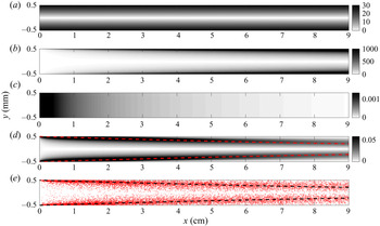


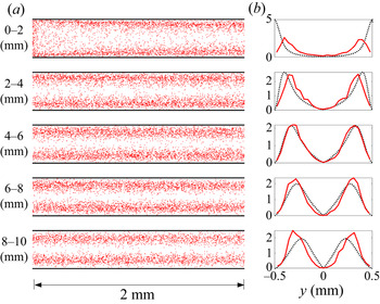


 Open access