


1. Introduction
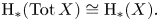
The Mayer–Vietoris spectral sequence, a generalization of the well-known Mayer–Vietoris long exact sequence, is an effective and far-reaching construction in algebraic topology. In its classical form, the Mayer–Vietoris spectral sequence is built from the intersection patterns of a cover of a given topological space $X$ . This spectral sequence converges to the homology of $X$
 , thus providing a powerful tool in various topological and combinatorial applications. First and foremost, it is related to the classical Nerve lemma (cf. theorem 3.9). A proof of the Nerve lemma using a spectral sequence argument appeared in [Reference Segal37, Section 5], and has since been generalized in several ways. More recently, the Nerve lemma and the Mayer–Vietoris spectral sequence have been receiving increasing attention due to their applications in persistent homology [Reference Bauer, Kerber, Roll and Rolle5, Reference Casas.9, Reference Guidolin and Landi25, Reference Govc and Skraba27, Reference Lipsky, Skraba and Vejdemo-Johansson35], bounded cohomology [Reference Frigerio and Maffei21, Reference Ivanov30], homology of configuration spaces [Reference Chettih14–Reference Chen, Lü and Wu16], and topological complexity of spaces [Reference Basu3, Reference Lütgehetmann and Recio-Mitter34]. Classically, a description of the $E^2$
 -page was used to infer properties of spherical arrangements [Reference Jewell31, Reference Jewell, Orlik and Shapiro32], and to study hyperplane arrangements in general [Reference Björner and Ekedahl4, Reference Davis and Settepanella18, Reference Denham, Suciu and Yuzvinsky19].
The Nerve lemma holds for ‘good covers’ of simplicial complexes (or, more generally, topological spaces), i.e. covers whose elements and all of their possible finite intersections are contractible. When such intersections are not contractible, nor acyclic, the conclusion of the Nerve lemma does not generally hold. Regardless, the Mayer–Vietoris spectral sequence eventually converges to the homology of $X$ , and the pages of the spectral sequence provide an increasingly accurate approximation of this convergence. Therefore, subcomplexes of the pages of the spectral sequence should contain interesting invariants – e.g. other homology theories, as for path homology [Reference Asao2], or torsion, as in [Reference Jewell31] – which suggests the following question:
Question Let $\mathcal {U}$ be a cover of a topological space $X$
 . Which topological properties of $X$
 , or combinatorial properties of the nerve of $\mathcal {U}$
 , can be read from the second page of the Mayer–Vietoris spectral sequence?
As stated, this question is rather vague, as it strongly depends on both the cover $\mathcal {U}$ and the space $X$
 . In this paper, we focus on the cover $\mathcal {U}^{\mathrm {ast}}$
 consisting of anti-star subcomplexes $\mathrm {ast}_X(v)$
 of a finite, connected, simplicial complex $X$
 ; here $v$
 runs across the vertices of $X$
 , and $\mathrm {ast}_X(v)$
 is the complement of the star of $v$
 in $X$
 (cf. definition 3.11). Our main result is that the second page of the Mayer–Vietoris spectral sequence of $X$
 , with respect to the cover $\mathcal {U}^{\mathrm {ast}}$
 , is related to another combinatorial and homological invariant $\ddot {\mathrm {B}} (X)$
 of simplicial complexes:
Theorem 1.1 Let $X$ be a finite simplicial complex with $m$
 vertices. Then, for all $i\geq 0$
 and $0\leq j\leq m$
 , there exists an isomorphism of bigraded modules
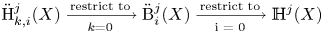
between the second page of the augmented Mayer–Vietoris spectral sequence of ${X}$ , associated with the anti-star cover, and the $0$
 -th degree überhomology of $X$
 .
.
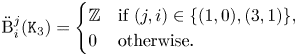
The bigraded homology $\ddot {\mathrm {B}}^j_i (X)$ is the zero-degree specialization of a more general homology theory of simplicial complexes introduced in [Reference Celoria12]. The latter theory is called the überhomology of $X$
 . It was shown in [Reference Celoria12] that überhomology contains both topological and combinatorial information about finite simplicial complexes. Theorem 1.1 clarifies that, when setting one of the degrees to $0$
 , the überhomology theory reads off combinatorial information of $X$
 from the second page of the associated spectral sequence. It would be interesting to compare theorem 1.1 with the results of [Reference Everitt and Turner20]. In that paper, a cellular-type cohomology associated with Boolean covers of a lattice is presented. A Mayer–Vietoris spectral sequence is used to relate the homology of a Boolean cover to the homology of the underlying lattice. In their case, the cover corresponds to the upper intervals containing the atoms of the lattice, suggesting a parallel combinatorial interpretation of the Mayer–Vietoris spectral sequence in that context.
Using the correspondence in theorem 1.1, we provide some computations, and extend previous results of [Reference Caputi, Celoria and Collari10, Reference Celoria12] first obtained via direct computations or discrete Morse theory techniques – cf. propositions 5.2 and 5.7. We investigate the effect of coning and suspending. A further specialization of überhomology, called bold homology, is related to connected dominating sets. We further prove that the $0$ -degree überhomology of flag complexes on triangle-free graphs is completely determined by their bold homology (proposition 5.6).
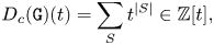
Counting connected dominating sets in a graph is a NP-hard problem. It was shown in [Reference Caputi, Celoria and Collari10] that bold homology yields a categorification of the connected domination polynomial. Denote by $D_c({\tt G})$ the connected domination polynomial of a graph ${\tt G}$
 (see equation (2.4)). The definition of the anti-star cover can be extended to regular CW-complexes, and our main application of theorem 1.1 is the following:
Theorem 1.2 Let $X\neq \Delta ^n$ be a finite, connected, regular CW-complex. Assume that the anti-star cover of $X$
 is a $1$
 -Leray cover, and that the $1$
 -skeleton of $X$
 is a simple graph ${\tt G}$
 . Then, we have

where $m$ is the number of vertices in $X$
 .
.
Theorem 1.2, which is almost a straightforward consequence of theorem 1.1 in the case of simplicial complexes, is less direct when considering CW-complexes. For CW-complexes, a definition of überhomology and bold homology groups is missing, and the bridge to dominating sets unclear. The role of theorem 1.2 is to clarify this connection. For example, using the more general framework of CW-complexes, we are able to infer that $-1$ is a root of the connected domination polynomial of grid graphs (cf. corollary 5.4).
Our last application concerns chordal graphs. Recall that a chordal graph is a graph ${\tt G}$ in which each induced cycle, i.e. a cycle that is an induced subgraph of ${\tt G}$
 , has exactly three vertices.
Corollary 1.3 Let ${\tt G}$ be a chordal graph on $m\geq 3$
 vertices. Then, $-1$
 is a root of the connected domination polynomial $D_c({\tt G})$
 .
.
Examples of non-chordal graphs ${\tt G}$ for which $-1$
 is a root of $D_c({\tt G})$
 are, for example, grid graphs (cf. corollary 5.4). In these cases, the converse of corollary 1.3 does not hold. It would be interesting to further explore the relation between topological properties of simplicial complexes and combinatorial properties of their $1$
 -skeleta, especially in relation with general notions of chordality [Reference Adiprasito, Nevo and Samper1].
2. Überhomology, its 0-degree, and bold homology
We start by recalling the definition of überhomology, following [Reference Caputi, Celoria and Collari10, Reference Celoria12].
Let $X$ be a finite and connected simplicial complex with $m$
 vertices, say $V(X)=\{v_1,\,\dots,\,v_m\}$
 . In what follows, we assume that the vertices of $X$
 are given a fixed order. The choice of such ordering is auxiliary and will not affect the following discussion.
A bicolouring $\varepsilon$ on $X$
 is a map $\varepsilon \colon V(X) \to \{0,\,1\}$
 . As a visual aid, we will sometimes identify $0$
 with white and $1$
 with black. A bicoloured simplicial complex is a pair $(X,\,\varepsilon )$
 , consisting of a simplicial complex $X$
 equipped with the bicolouring $\varepsilon$
 . Given a $n$
 -dimensional simplex $\sigma$
 in $(X,\,\varepsilon )$
 , define its weight with respect to $\varepsilon$
 as the sum
Equivalently, $w_\varepsilon (\sigma )$ is the number of $0$
 /white-coloured vertices in $\sigma$
 . For a fixed bicolouring $\varepsilon$
 , the weight in equation (2.1) induces a filtration of the simplicial chain complex $C_*(X;\mathbb {Z}_2)$
 associated with $X$
 . More explicitly, set

The simplicial differential $\partial$ respects this filtration; it can be decomposed as the sum of two differentials (cf. [Reference Celoria12, Lemma 2.1]); one which preserves the weight, denoted by $\partial _h$
 , and one which decreases the weight by one. Call $(C(X,\,\varepsilon ),\,\partial _h)$
 the bigraded chain complex, whose underlying module is $C(X;\mathbb {Z}_2)$
 ; the first degree is given by simplices’ dimensions, while the weight $w_\varepsilon$
 gives the second. The $\varepsilon$
 -horizontal homology $\mathrm {H}^h(X,\,\varepsilon )$
 of $(X,\,\varepsilon )$
 is the homology of the bigraded chain complex $(C(X,\,\varepsilon ),\,\partial _h)$
 . In other words, $\mathrm {H}^h(X,\,\varepsilon )$
 is the homology of the graded object associated with the filtration $\mathscr {F}_j (X,\, \varepsilon )$
 .
.
The next step towards the definition of the überhomology is to note that the bicolourings on $X$ can be canonically identified with elements of Boolean poset $B(m)$
 on a set with $m$
 elements (partially ordered by inclusion). Let $\varepsilon$
 and $\varepsilon '$
 be two bicolourings on $X$
 differing only on a vertex $v_i$
 ; assume further that $\varepsilon (v_i) = 0$
 and $\varepsilon '(v_i) =1$
 . Denote by $d_{\varepsilon, \varepsilon '}$
 the weight-preserving part of the identity map $\mathrm {Id} \colon \mathrm {H}^h(X,\,\varepsilon ) \to \mathrm {H}^h(X,\,\varepsilon ')$
 . With a slight abuse of notation, $d_{\varepsilon, \varepsilon '}$
 can be written as

see [Reference Celoria12, Section 6]. Note that the latter case can only occur if $w_{\varepsilon }(\sigma ) = w_{\varepsilon '}(\sigma )-1$ .
.
For a given bicolouring $\varepsilon$ on $X$
 , set $\ell (\varepsilon ) := \sum _{j} \varepsilon (v_j)$
 . The $j$
 -th über chain module is then defined as follows:
By [Reference Celoria12, Proposition 6.2], the map
is a differential of degree $1$ , turning $(\ddot {\mathrm {C}}^{*}(X;\mathbb {Z}_2),\, \ddot {d})$
 into a cochain complex. A schematic summary for the construction of the über chain complex is presented in figure 1.
Definition 2.1 The überhomology $\ddot {\mathrm {H}}^*(X)$ of a finite and connected simplicial complex $X$
 is the homology of the complex $(\ddot {\mathrm {C}}^{*}(X;\mathbb {Z}_2),\, \ddot {d})$
 .
.
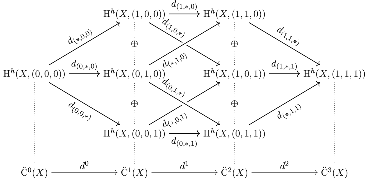
Figure 1. Boolean poset $B(3)$ with vertices decorated by the horizontal homologies of a simplicial complex with $3$
 vertices, and its ‘flattening’ to the über chain complex.
Überhomology groups can be endowed with two extra gradings, yielding a triply graded module. Indeed, the differential $\ddot {d}$ preserves both the simplices’ weight and dimension. The notation for the three gradings on the überhomology is as follows: $\ddot {\mathrm {H}}^j_{k,i}(X)$
 denotes the component of the homology generated by simplices of dimension $i$
 , with $k$
 vertices of colour $0$
 , and whose (über)homological degree is $j$
 .
.
The above definition can be rephrased in terms of poset homology [Reference Caputi, Collari and Di Trani11, Reference Chandler13], which allows extending the definition of überhomology from $\mathbb {Z}_2$ to more general coefficients:
Proposition 2.2 [Reference Caputi, Celoria and Collari10, Proposition 2.14]
Let $X$ be a connected simplicial complex with $m$
 vertices, and $\mathbf {Mod}_{R}$
 the category of $R$
 -modules over a commutative ring $R$
 . Then, the überhomology of $X$
 with coefficients in $R$
 coincides with the poset homology of $B(m)$
 , with coefficients in a suitable functor $\mathcal {H}\colon {B}(m)\to \mathbf {Mod}_{R}$
 .
.
We refer to [Reference Caputi, Celoria and Collari10] for the proof of proposition 2.2, and for a more detailed account of the poset homology interpretation.
As mentioned above, the überdifferential $\ddot {d}$ preserves the $(k,\,i)$
 -bidegree. In particular, specializing to the component of überhomology of weight $0$
 yields a bigraded homology.
Definition 2.3 For a simplicial complex $X$ , define the $0$
 -degree überhomology to be the bigraded homology
An alternative definition of $\ddot {\mathrm {B}}(X)$ is the following; for $\varepsilon \in \mathbb {Z}_2^m$
 define $X_\varepsilon$
 to be the simplicial subcomplex of $X$
 induced by the $1$
 -coloured vertices with respect to $\varepsilon$
 . The homology $\ddot {\mathrm {B}}^*_i(X)$
 is obtained by decorating each vertex $\varepsilon$
 in Boolean poset $B(m)$
 with the $i$
 -th homology $\mathrm {H}_i (X_\varepsilon )$
 of $X_\varepsilon$
 ; the differentials associated with the cube's edges are induced by inclusion. This is to say that $\ddot {\mathrm {B}}^*_i(X)$
 is the poset homology on Boolean poset $B(m)$
 with coefficients in the functor given by simplicial homology in dimension $i$
 .
.
Using proposition 2.2, the definition of $\ddot {\mathrm {B}}^*_*$ can be extended to encompass general coefficients; set $\ddot {\mathrm {B}}^j_i(X;R)$
 for the $0$
 -degree überhomology of $X$
 , with coefficients in a commutative ring $R$
 .
.
Example 2.4 As an example, we can compute the homology $\ddot {\mathrm {B}}^j_i(\partial \Delta ^2)$ of the boundary of $\Delta ^2$
 . The chain complex for is shown in figure 2. This complex is concentrated in homological degrees between $1$
 and $3$
 , and simplicial degrees $0$
 and $1$
 . In degree $i=0$
 , it is isomorphic to the simplicial chain complex associated with $\partial \Delta ^{2}$
 , while in degree $i=1$
 there are only trivial differentials, and a unique non-trivial summand in degree $j=3$
 . It follows that
More explicitly, the generator in bidegree $(1,\,0)$ is spanned by the direct sum of the three connected components identified by a single black vertex (see the first column of figure 2). The other generator can instead be identified with the fundamental class of $\partial \Delta ^2$
 , regarded as a triangulation of $S^1$
 .
.
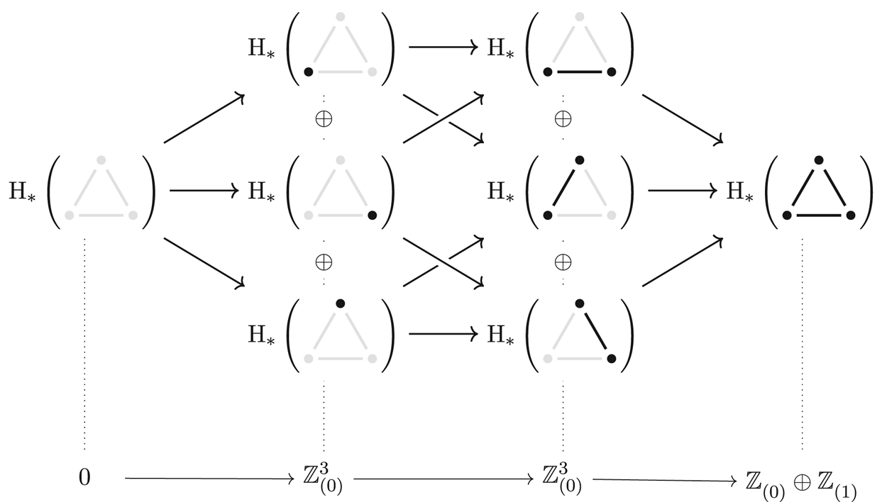
Figure 2. The $0$ -degree überchain complex of $\partial \Delta ^2$
 . Here $\mathbb {Z}^{d}_{(i)}$
 denotes a $\mathbb {Z}^d$
 summand in $\ddot {\mathrm {B}}^{*}_{i}$
 .
.
2.1 Bold homology
The specialization of $\ddot {\mathrm {B}}^*_i(X)$ to $i=0$
 is known as bold homology, and is denoted by $\mathbb {H}^* (X)$
 . This homology was introduced in [Reference Celoria12, Section 8], and it was shown to contain non-trivial combinatorial information on simple graphs [Reference Caputi, Celoria and Collari10]. The relations between the three homologies introduced so far can be schematically summarized as follows:
Let ${\tt G}$ be a connected simple graph, that is, a connected $1$
 -dimensional simplicial complex. A subset $S\subseteq V({\tt G})$
 of the vertices of ${\tt G}$
 is called
• dominating if each vertex in $V({\tt G})$
 either belongs to $S$ or shares an edge with some element of $S$;
• connected if $S$
spans a connected subcomplex.


The connected domination polynomial of a graph ${\tt G}$ is defined as
where $S$ ranges among connected dominating sets in $V({\tt G})$
 . Computing the connected domination polynomial of a graph is known to be NP-hard [Reference Garey and Johnson23]. In [Reference Caputi, Celoria and Collari10], the authors prove the existence of a tight relation between connected domination polynomials and the bold homology's Euler characteristic:
Theorem 2.5 [Reference Caputi, Celoria and Collari10, Theorem 1.2]
The bold homology categorifies $D_c(-1)$ . More precisely, $\mathbb {H}^*$
 is functorial under inclusion of graphs, and its Euler characteristic is $D_c(-1)$
 .
.
From this result, some properties and computations of $\mathbb {H}$ can be deduced. For example, the bold homology of trees is zero, and it detects complete graphs (see [Reference Caputi, Celoria and Collari10] for the precise statements). Computations performed with bold homology can be extended to simplicial complexes as well; indeed, the following can be deduced at once from the definitions:
Lemma 2.6 Let $X$ be a simplicial complex, and $X^{(1)}$
 its $1$
 -skeleton. Then, there exists a graded isomorphism $\mathbb {H}^*(X) \cong \mathbb {H}^*(X^{(1)})$
 .
.
Proof. Connected components of $1$ -coloured subcomplexes in $X^{(1)}$
 are in canonical bijection with connected components in $X$
 . Then, the result follows by [Reference Caputi, Celoria and Collari10, Theorem 1.3].
3. Anti-star covers and spectral sequences
One of the main tools employed in (co)homology computations is the generalization of the Mayer–Vietoris long exact sequence in terms of spectral sequences. To set the notations, we start by recalling some basic definitions, referring to [Reference McCleary36] for further details.
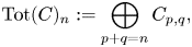
We will focus on augmented first quadrant spectral sequences of homological type, i.e. spectral sequences arising from first-quadrant augmented bicomplexes, whose induced differentials have bidegree $(-r,\,r-1)$ . By a first quadrant augmented bicomplex $(C_{p,q},\,\delta _{p,q})$
 of bidegree $(a,\,b)$
 we mean a bigraded $R$
 -module $C_{p,q}$
 with differentials
where $C_{p,q}=0$ for $p<-1$
 and $q<0$
 . Spectral sequences arise naturally in the context of filtered chain complexes. As customary, we say that a spectral sequence $(E^r,\,d^r)$
 converges to a graded module $\mathrm {H}_*$
 , and write $E_{p,q}\Rightarrow \mathrm {H}_{p+q}$
 , if there is a filtration $F$
 on $\mathrm {H}_*$
 such that $E^{\infty }_{p,q}\cong \mathrm {Gr}_{p,q}\mathrm {H}_*$
 for all $p,\,q$
 , where $E^{\infty }_{p,q}$
 is the limit term of the spectral sequence.
We now specialize to first quadrant augmented bicomplexes $(C,\,\delta _v,\,\delta _h)$ where $\delta _v$
 and $\delta _h$
 are differentials of bidegrees $(0,\,-1)$
 and $(-1,\,0)$
 , respectively, and $\delta _v\circ \delta _h=\delta _h\circ \delta _v$
 . Consider the associated total complex
with differential $\delta$ defined by setting $\delta (x):=\delta _h(x)+(-1)^p\delta _v(x)$
 for each $x\in C_{p,*}$
 , and each $p$
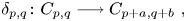
 . There are two natural filtrations on $\operatorname {\mathrm {Tot}} (C)$
 . The first filtration $F^I$
 is defined by cutting the direct sum above at the $p$
 -level: $F^I_p(\operatorname {\mathrm {Tot}} (C))_n:= \bigoplus _{i\leq p} C_{i,n-i}$
 . The second filtration $F^{II}$
 is the complementary one: $F^{II}_q(\operatorname {\mathrm {Tot}}(C))_n:=\bigoplus _{j\leq q} C_{n-j,j}$
 . In the special case of a first quadrant double chain complex, both filtrations are bounded (from above and below), hence both the associated spectral sequences converge to the homology of the total complex $\operatorname {\mathrm {Tot}}(C)$
 . The $0$
 -page of the spectral sequence arising from the first filtration is

and for the second filtration is:

The differentials are respectively induced by $\delta _v$ and by $\delta _h$
 . The first pages of the associated spectral sequences are given by $IE^1_{p,q}=\mathrm {H}_q(C_{p,*})$
 , with induced differential $\delta ^{(2)}_h$
 , and by $IIE^1_{p,q}=\mathrm {H}_q(C_{*,p})$
 , with induced differential $\delta _v^{(2)}$
 , simply denoted by $\delta ^{(2)}$
 in the follow-up, respectively.
3.1. The Mayer–Vietoris spectral sequence
Following [Reference Brown8, Chapter VII.4] and [Reference Godement26, Sections I.3.3 and II.5], we briefly recall the construction of the Mayer–Vietoris spectral sequence.
For a simplicial complex $X$ , denote by $P(X)$
 the face poset of $X$
 , i.e. the poset of non-empty simplices of $X$
 , ordered by inclusion. Let $X_p$
 be the set consisting of the $p$
 -simplices in $X$
 , and assume that the set of vertices is always finite and ordered. The results will not depend on the choice of ordering.
Let $\mathcal {U}=\{U_i\}_{i\in I}$ be a simplicial cover of $X$
 , i.e. a family of subcomplexes of $X$
 with the property that each $U_i$
 is non-empty and $\bigcup _{i\in I}U_i=X$
 . For each non-empty subset $J$
 of the set of indices $I$
 , denote by $U_{J}$
 the intersection $\bigcap _{j\in J} U_j$
 of the corresponding elements in the cover. From this data, we can associate to $X$
 another simplicial complex:
Definition 3.1 Given a simplicial complex $X$ and cover $\mathcal {U}=\{U_i\}_{i\in I}$
 , the nerve $\operatorname {\mathrm {N}} (\mathcal {U})$
 is the simplicial complex on the family of non-empty finite subsets $J\subseteq I$
 , such that $U_{J}:= \bigcap _{j\in J} U_j \neq \emptyset$
 .
.
Consider the cover $\mathcal {U}=\{U_i\}_{i\in I}$ of $X$
 . We can associate to each simplex $\sigma$
 with $\operatorname {\mathrm {N}} (\mathcal {U})$
 a subset $J$
 of $\{ 1,\,\ldots,\, \vert I\vert \}$
 . In particular, for a $p$
 -simplex $\sigma$
 of $\operatorname {\mathrm {N}} (\mathcal {U})$
 , defined by the indices $j_0,\, \dots,\, j_p$
 , we will denote by $U_\sigma$
 the intersection $U_{j_0}\cap \dots \cap U_{j_p}$
 .
.
Every poset is a category. In particular, this holds for the face poset $P(X)$ ; its objects are the simplices of $X$
 , and there is a morphism $\tau \to \sigma$
 whenever $\tau$
 is a face of $\sigma$
 . Denote the category obtained this way by $\mathbf {P}(X)$
 , and by $\mathbf {Ab}$
 the category of Abelian groups.
Definition 3.2 A coefficient system on $X$ is a functor $\mathcal {L}\colon \mathbf {P}(X)^\mathrm {op}\to \mathbf {Ab}$
 .
.
More concretely, a coefficient system on $X$ is a family of Abelian groups $\{A_{\sigma }\}$
 , indexed by the simplices $\sigma$
 of $X$
 , together with a map $A_{\tau \subseteq \sigma }\colon A_{\sigma }\to A_{\tau }$
 whenever $\tau$
 is a face of $\sigma$
 , and such that $A_{\tau \subseteq \sigma }\circ A_{\mu \subseteq \tau }=A_{\mu \subseteq \sigma }$
 if $\mu \subseteq \tau \subseteq \sigma$
 .
.
Example 3.3 Let $\mathcal {U}$ be a cover of a simplicial complex $X$
 . For each $q \in \mathbb {N}$
 and $\sigma \in \operatorname {\mathrm {N}}(\mathcal {U})$
 , define
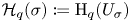
as the $q$ -th homology group of the subcomplex $U_\sigma$
 of $X$
 . If $\tau$
 is a face of $\sigma$
 belonging to $\operatorname {\mathrm {N}}(\mathcal {U})$
 , then there is an inclusion $U_{\sigma }\subseteq U_{\tau }$
 , hence an induced map between the associated $q$
 -homology groups. It is straightforward to check that $\mathcal {H}_q$
 yields a coefficient system on the nerve $\operatorname {\mathrm {N}}(\mathcal {U})$
 . Analogously, the group $C_q(U_\sigma )$
 of $q$
 -chains in $U_\sigma$
 can be considered; this also yields a coefficient system $\mathcal {C}_q$
 on $\operatorname {\mathrm {N}}(\mathcal {U})$
 .
.
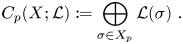
Given a simplicial complex $X$ and a coefficient system $\mathcal {L}$
 on $X$
 , it is possible to define the homology groups of $X$
 with coefficients in $\mathcal {L}$
 , cf. [Reference Godement26, Section I.3.3]. For each $n\geq 0$
 , define the $p$
 -chains as the sum
If $\sigma$ is the simplex $[x_0,\, \dots,\, x_p]$
 , then set $d_i(\sigma ):= [x_0,\, \dots,\, \widehat {x_i},\, \dots,\, x_p]$
 for its $i$
 -th face. By functoriality of $\mathcal {L}$
 , there are restriction maps
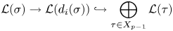
for all $\sigma \in X_p$ and $0\leq i\leq p$
 , extending to maps $\partial _i\colon C_p(X;\mathcal {L})\to C_{p-1}(X;\mathcal {L})$
 on the whole chain complex $C_p(X;\mathcal {L})$
 , for each $i$
 . The differential $\partial \colon C_p(X;\mathcal {L})\to C_{p-1}(X;\mathcal {L})$
 is defined by setting $\partial := \sum _{i=0}^p (-1)^i\partial _i$
 . This is usually known as Čech differential, and the resulting chain complex is usually called cosheaf complex (see e.g. [Reference Bredon7, Section 4]).
Definition 3.4 The homology of $X$ with coefficients in the coefficient system $\mathcal {L}$
 is the homology of the chain complex $(C_*(X;\mathcal {L}),\,\partial )$
 .
.
We now turn to the construction of the Mayer–Vietoris spectral sequence. This is the spectral sequence associated to a double chain complex, corresponding to a cover of a topological space. For a simplicial complex $X$ and cover $\mathcal {U}$
 , set
, set
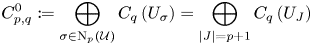
for the $\mathbb {Z}$ -module freely generated by the $q$
 -chains of the subcomplexes of $X$
 obtained considering intersections of $p+1$
 elements of the cover $\mathcal {U}$
 . There are two differentials, decreasing either the $p$
 or the $q$
 degree. Denote by $\delta ^0_h\colon C^0_{p,q}\to C^0_{p-1,q}$
 the horizontal differential decreasing the $p$
 -degree, and by $\delta ^0_v\colon C^0_{p,q}\to C^0_{p,q-1}$
 the vertical one decreasing the $q$
 -degree. As customary, we define the differential $\delta ^0_v$
 as the alternating sum over the faces: if $\tau =[v_0,\,\dots,\, v_q]$
 , then $\delta ^0_v(\tau ):= \sum _{k=0}^q(-1)^k[v_0,\,\dots,\,\widehat {v_k},\,\dots,\, v_q]$
 . This way, for all $p\geq 0$
 , we get chain complexes $(C^0_{p,*},\,\delta ^0_v)$
 . In the horizontal direction instead, at a fixed $q\in \mathbb {N}$
 , we define $\delta _h^0$
 as the differential of the chain complex $C_p(\operatorname {\mathrm {N}}(\mathcal {U}); \mathcal {C}_q)$
 of $\operatorname {\mathrm {N}}(\mathcal {U})$
 with coefficients in the coefficient system $\mathcal {C}_q$
 . More concretely, for each $J$
 appearing in the sum of equation (3.1), and each $j\in J$
 , the subset $J':= J\setminus \{j\}$
 is a face of $J$
 in $\operatorname {\mathrm {N}}(\mathcal {U})$
 . The inclusion of $J'$
 in $J$
 induces a simplicial map $U_{J}\to U_{J'}$
 (reversing the ordering), hence a map on the level of $q$
 -chains. Then, the differential $\delta ^0_h$
 is defined on the basis elements of $C_q(U_J)$
 as the alternating sum of $U_{J\setminus \{j\}}$
 over $j \in J$
 . This definition is then extended to all sums by linearity.
Remark 3.5 The differentials $\delta _h^0$ and $\delta _v^0$
 commute, i.e. $\delta _h^0\circ \delta _v^0=\delta _v^0 \circ \delta _h^0$
 .
.
Endowing the groups $C^0_{p,q}$ with the differentials $\delta _h^0$
 and $\delta _v^0$
 , yields a double chain complex. Both spectral sequences associated with the double chain complex $(C^0_{*,*},\, \delta _h^0,\, \delta _v^0)$
 (corresponding to the vertical and horizontal filtration) converge to the homology of the total chain complex $\operatorname {\mathrm {Tot}} X$
 , since $(C^0_{*,*},\, \delta _h^0,\, \delta _v^0)$
 is a first quadrant double chain complex. However, even though the two spectral sequences abut to the same graded object $\mathrm {H}_*(\operatorname {\mathrm {Tot}} X)$
 , they have different $E^\infty$
 -terms – seen as bigraded objects. First, consider the spectral sequence $IE$
 obtained by taking homology with respect to the $p$
 -degree. As, for $s>0$
 fixed, the chain complexes $C_{*,s}^0$
 are acyclic [Reference Brown8, Section VII.4], its $E^1$
 -page has non-trivial groups $C_s(X)$
 concentrated in the first column. The differential is induced from $\delta ^0_v$
 . Hence, the second page consists of the homology groups $\mathrm {H}_*(X)$
 . Therefore, this spectral sequence collapses at the second page, yielding
The second spectral sequence $IIE$ is called the Mayer–Vietoris spectral sequence. From now on, we will simply write $E$
 instead of $IIE$
 .
.
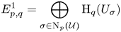
Definition 3.6 The first page of the Mayer–Vietoris spectral sequence associated with a simplicial complex $X$ and cover $\mathcal {U}$
 is given by
with differential $\delta ^{(1)}\colon E^1_{p,q}\to E^1_{p-1,q}$ induced by $\delta ^0_h$
 .
.
Remark 3.7 The group $E^1_{p,q}$ in equation (3.3) coincides with the chain group $C_p(\operatorname {\mathrm {N}}(\mathcal {U});\mathcal {H}_q)$
 , where $\mathcal {H}_q$
 is the coefficient system described in example 3.3.
Then, the $E^2$ -page of $IIE$
 is given by
As previously remarked, this spectral sequence converges to the homology of the total complex $\operatorname {\mathrm {Tot}} X$ . Therefore, we get convergence of the Mayer–Vietoris spectral sequence to the homology of $X$
 by equation (3.2).
Remark 3.8 Assume that the elements of the cover of $X$ have homology $\mathrm {H}_i(U_\sigma )=0$
 for all $\sigma$
 and $i\geq k$
 . Then, the differential $\delta ^{i}$
 on the $i$
 -th page must be trivial for $i\geq k+2$
 . Thus, in such a case, the Mayer–Vietoris spectral sequence converges at the page $E^{k+2}$
 .
.
As a consequence, if each $U_\sigma$ is acyclic, the described spectral sequence collapses at the second page (furthermore, it has non-zero groups only at $q=0$
 ), and we recover the classical Nerve lemma – cf. [Reference Brown8, Theorem VII (4.4)]:
Theorem 3.9 (Nerve lemma)
Let $X$ be a finite simplicial complex, $\mathcal {U}$
 a cover by subcomplexes, and suppose that every non-empty intersection $U_\sigma$
 is acyclic. Then, $\mathrm {H}_*(X)\cong \mathrm {H}_*(\operatorname {\mathrm {N}}(\mathcal {U}))$
 .
.
When the subcomplexes $U_\sigma$ are not acyclic, the conclusion of the Nerve lemma does not hold. Nonetheless, the Mayer–Vietoris spectral sequence eventually converges to the homology of $X$
 .
.
Remark 3.10 The results outlined in this section are a special case of a more general construction. Let $\mathcal {F}$ be a sheaf on a topological space $X$
 . If $\mathcal {U}$
 is a cover of $X$
 which is $\mathcal {F}$
 -acyclic (i.e. $\mathcal {F}$
 is acyclic on the finite intersections of $\mathcal {U}$
 ), then the Čech cohomology of $\mathcal {U}$
 with coefficients in $\mathcal {F}$
 coincides with the sheaf cohomology of $X$
 . Furthermore, if $\mathcal {U}$
 consists of two open subsets of $X$
 , we recover the classical Mayer–Vietoris sequence for the sheaf $\mathcal {F}$
 .
.
3.2 The anti-star cover
For our purposes, it is particularly interesting to consider a special type of covers of simplicial complexes. These covers are obtained from complements of vertex stars, and are commonly known as anti-star covers. Let $X$ be a simplicial complex which is not the standard simplex $\Delta ^m$
 .
.
Definition 3.11 For each vertex $v$ in $X$
 , denote by $\mathrm {ast}_X(v)$
 the subcomplex of $X$
 spanned by the vertices in $V(X)\setminus \{v\}$
 . The associated cover $\mathcal {U}^{\mathrm {ast}}_X=\{\mathrm {ast}_X(v)\}_{v\in V(X)}$
 is called the anti-star cover of $X$
 .
.
Equivalently, each $\mathrm {ast}_X(v)$ is obtained from $X$
 by removing the open star of $v$
 . When clear from the context, we will drop the dependency on $X$
 and simply write $\mathrm {ast}(v)$
 and $\mathcal {U}^{\mathrm {ast}}$
 . Anti-star subcomplexes contain homotopical information about the simplicial complex $X$
 . Indeed, if the inclusions in the (anti-)star is null-homotopic, if $\mathrm {ast}_X(v)$
 is homotopy equivalent to a wedge of $n$
 -dimensional spheres, and the link $\mathrm {lk}_X(v)$
 is homotopy equivalent to a wedge of $(n-1)$
 -dimensional spheres, then $X$
 is homotopy equivalent to a wedge of $n$
 -dimensional spheres [Reference Vrećica and Živaljević40, Lemma 5]. Furthermore, if $v$
 is a (non-isolated) vertex of $X$
 , there is a Mayer–Vietoris long exact sequence

relating the (reduced) homology of $X$ , of the link of $v$
 and of the associated anti-star complex. When multiple vertices are considered at once, long exact sequences are not sufficient to determine the homology of $X$
 , and the Mayer–Vietoris spectral sequence comes into play.
Remark 3.12 The nerve associated with the anti-star cover can be easily seen to coincide with the standard simplex $\Delta ^m$ .
.
In order to showcase some of the techniques used in §5, some sample computations of the Mayer–Vietoris spectral sequence associated with the anti-star cover are provided below.
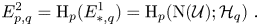
Example 3.13 Let $X = \partial \Delta ^2$ , as shown in figure 3. Let $U_i=\mathrm {ast}(v_i)$
 be the anti-star subcomplexes, so $U_i=[v_{i+1},\,v_{i+2}]$
 , with indices modulo $3$
 . The intersection $U_i\cap U_{i+1}$
 is given by the vertex $v_{i+2}$
 . Adding to $\mathcal {U}^{\mathrm {ast}}$
 the empty and the complete intersections as well, produces the Boolean poset represented in figure 4. Applying the homology functor $\mathrm {H}_q$
 to each element of the poset, yields instead the decorated cube in figure 5. The directions of the edges of the cube follow the inclusions; in turn, the $p$
 -differentials, are directed from the $p$
 -simplices of the associated nerve to the $(p-1)$
 -simplices.
Figure 3. The simplicial complex from example 3.13.
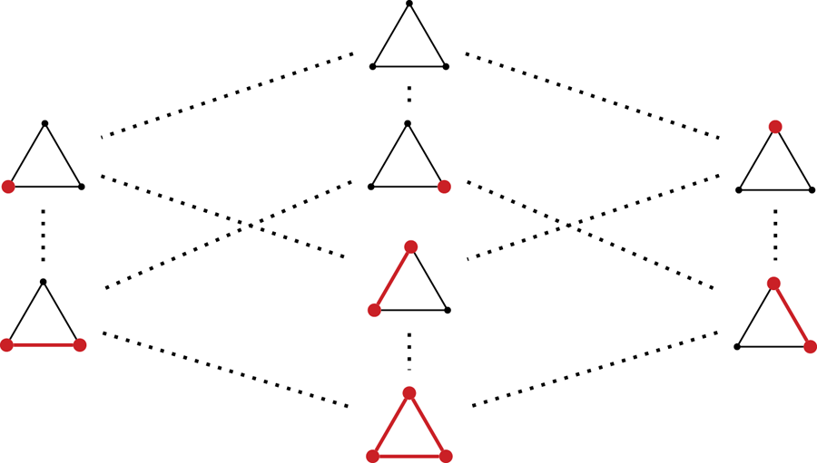
Figure 4. Boolean diagram associated with the nerve of the anti-star cover for $\partial \Delta ^2$ , with the empty and complete intersections added (top and bottom elements, respectively); red simplices denote the elements $U_i=\mathrm {ast}_X(v_i)$
 and their intersections (cf. with Fig. 2).
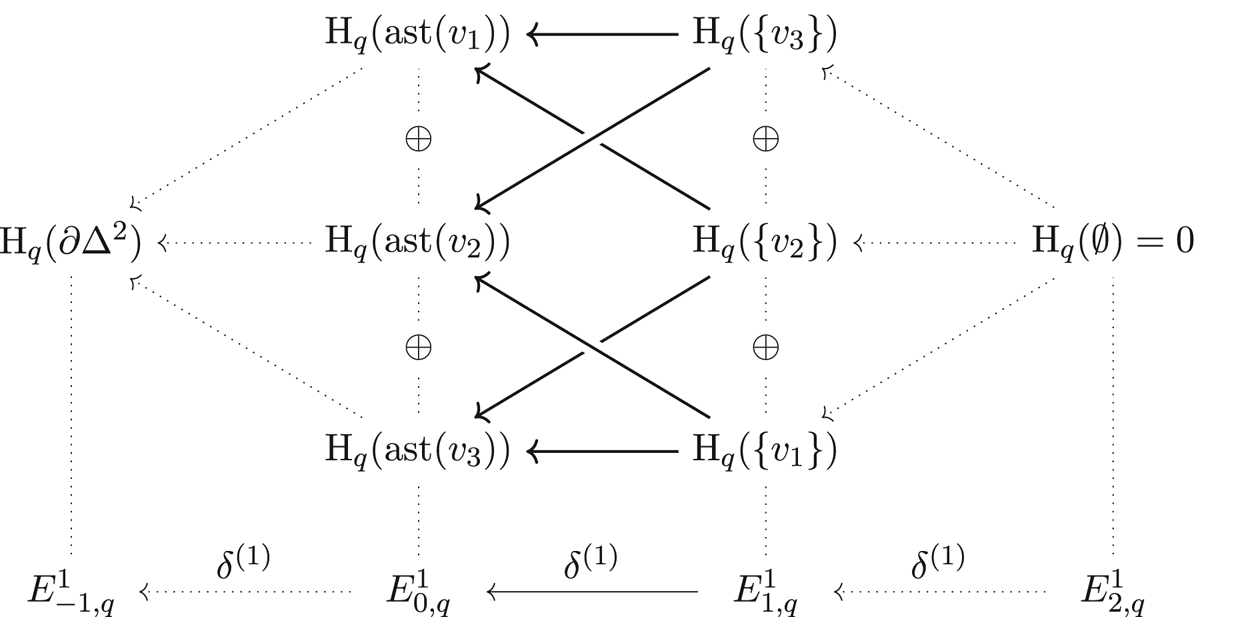
Figure 5. The coefficient system $\mathcal {H}_q$ on the nerve of $\partial \Delta ^2$
 , augmented by adding the values on the empty and complete intersections. The direct sum, columnwise, yields the $q$
 -th row of $E^1$
 in the Mayer–Vietoris spectral sequence.
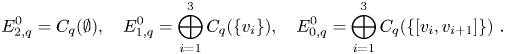
In order to get the double complex $E^0_{p,q}$ , for each $q$
 take the module generated by the $q$
 -chains, and then sum them up:
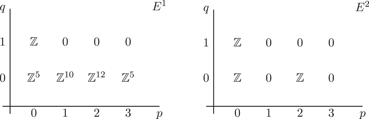
To turn to the first page, take the homology in the $q$ -direction; for each $q$
 , this results in the row shown at the bottom of figure 5.
The only non-trivial row is at $q=0$ . The unique differential has a non-trivial kernel of rank $1$
 . Taking the homology again, yields non-trivial homology groups $E^2_{0,0},\, E^2_{1,0}$
 , both isomorphic to $\mathbb {Z}$
 ; all other groups are zero. Concluding, the Mayer–Vietoris spectral sequence converges at the second page (as all differentials are zero), yielding non-trivial classes in homological dimension $0$
 and $1$
 ; this corresponds to the fact that $X$
 is homotopic to $S^1$
 .
.
Example 3.14 Consider the contractible simplicial complex $X$ shown in figure 6, i.e. the cone over a loop of length $4$
 . Then, as the Mayer–Vietoris spectral sequence converges to the homology of the disc, and all the subcomplexes $\mathrm {ast}(v_i)$
 , but $\mathrm {ast}(v_0)$
 , are contractible, the first and second page of the Mayer–Vietoris spectral sequence are the following:
The differential $\delta ^{(2)}\colon E^2_{2,0}\cong \mathbb {Z}\to \mathbb {Z}\cong E^2_{0,1}$ is non-trivial, and it kills the $\mathbb {Z}$
 -class at $E^2_{0,1}$
 . The third page contains only the homology of the point.
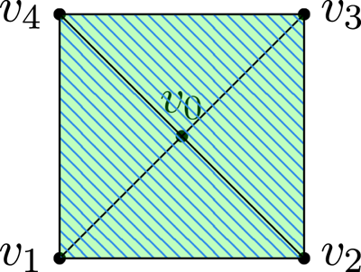
Figure 6. The cone over a loop of length four.
Example 3.15 Let $\Delta ^{n+1}$ be the standard $(n+1)$
 -simplex, considered with its standard triangulation. Let $S^n$
 be the sphere obtained by removing from $\Delta ^{n+1}$
 its interior. Then, the associated anti-star cover consists of contractible subcomplexes. Hence, the Mayer–Vietoris spectral sequence converges at the second page. As a consequence, $E^2$
 contains a rank one component in degree $(0,\,0)$
 , and one in degree $(n,\,0)$
 .
.
4. The overlap between Mayer–Vietoris and überhomology
The aim of this section is to prove theorem 1.1; or, more explicitly, to provide the identification between the second page of the Mayer–Vietoris spectral sequence associated with the anti-star cover and the $0$ -degree überhomology. To this end, the first step is to extend the computational framework of the Mayer–Vietoris spectral sequence to include the empty intersection of the elements of the cover as well.
Let $X$ be a simplicial complex, and let $\mathcal {U}^{\mathrm {ast}}$
 be its associated anti-star cover. Assume that $X$
 is not the standard simplex. By equation (3.3), the first page of the associated Mayer–Vietoris spectral sequence is

In order to include the empty intersection $U_\emptyset := X$ , it is possible to augment both the double chain complex $E^0_{p,q}$
 and the first page of the spectral sequence in degree $p=-1$
 with the homology of $X$
 , by setting
The horizontal differential of the first page, induced by inclusions, naturally extends to the $(-1)$ -column as well.
Definition 4.1 The augmented Mayer–Vietoris spectral sequence of $X$ relative to a cover $\mathcal {U}$
 is the spectral sequence with $E^1$
 -page given by $E^1_{p,q}=\bigoplus _{\sigma \in \mathrm {N}_p(\mathcal {U}^{ast})} \mathrm {H}_q(U_{\sigma })$
 , augmented in degree $-1$
 with $E^1_{-1,q}:= \mathrm {H}_q(X)$
 , and differentials induced by inclusions.
Remark 4.2 Consider the double chain complex $E^0_{p,q}$ , augmented in degree $p=-1$
 with $C_q(X)$
 ; i.e. set $E^0_{-1,q}:= C_q(X)$
 . As the rows of such augmented complex are exact [Reference Brown8, Section VII.4], by the acyclic assembly lemma [Reference Weibel41, Lemma 2.7.3], the total complex associated with $E^0_{*,*}$
 is acyclic. Hence, the augmented Mayer–Vietoris spectral sequence associated with (the second filtration of) $E^0_{*,*}$
 converges to an acyclic complex.
We provide some examples, extending those already discussed in §3.2.
Example 4.3 In parallel with example 3.13, consider the spectral sequence obtained by augmenting the first page in degree $-1$ with the homology of $X$
 . The first and second page now become the following:

The unique differential $\delta ^{(2)}\colon E^2_{1,0}\to E^2_{-1,1}$ is an isomorphism; hence, the third page is trivial. Analogously, for the square of example 3.14, the second page is completely trivial, except for the bidegrees $(0,\,1)$
 and $(2,\,0)$
 , where it is $\mathbb {Z}$
 .
.
Example 4.4 Consider the spheres from example 3.15. It is easy to see that the second page of the augmented Mayer–Vietoris spectral sequence is completely trivial, except for in degrees $(-1,\, n)$ and $(n,\, 0)$
 . The augmented spectral sequence collapses at page $n+1$
 .
.
We can now proceed with the proof of theorem 1.1;
Proof Proof of theorem 1.1
For a given set of vertices $\{v_{i_1},\,\dots,\, v_{i_k}\} \subseteq V(X)$ , the induced subcomplex
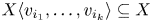
they span can be regarded as the ‘$1$ -coloured’ component of the complex $(X,\,\varepsilon )$
 , $\varepsilon$
 being the bicolouring on $X$
 assigning $1$
 to each $v_{i_j}$
 and $0$
 otherwise. Equivalently, $X \langle v_{i_1},\,\dots,\, v_{i_k}\rangle$
 is obtained by intersecting the anti-star subcomplexes $U_s$
 for all $s\notin \{i_1,\, \dots,\, i_k\}$
 .
.
Now observe that for a fixed $q\geq 0$ , by the definition of the chains in equation (2.2), restricted to the $0$
 -degree, we obtain an identification of the groups $E^1_{p,q}$
 with $\bigoplus _{\ell (\varepsilon )=m-p - 1} \mathrm {H}_q(X,\,\varepsilon )$
 ; this is the überhomological degree $m-p -1$
 component of the $0$
 -degree of the übercomplex. When restricting to the base field $R=\mathbb {Z}_2$
 , the $p$
 -differential coincides with the differential in equation (2.3). Furthermore, the agreement of the differentials extends to a general ring of coefficients $R$
 after choosing a sign assignment on the appropriate Boolean poset [Reference Caputi, Collari and Di Trani11]; the agreement does not depend on the choice of the sign assignment by proposition 2.2 and [Reference Caputi, Collari and Di Trani11, Theorem 3.16 and Corollary 3.18]. By definition 2.1, the homology of this chain complex is the überhomology of $X$
 . On the other hand, it yields the second page of the augmented Mayer–Vietoris spectral sequence. This gives the complete identification $E^2_{p,q}\cong \ddot {\mathrm {B}}^{m-p-1}_q(X)$
 for $p\geq -1$
 and $q\geq 0$
 .
.
In other words, the $0$ -degree überhomology of $X$
 coincides with the homology of the nerve of the anti-star cover, with coefficients in the functor $\mathcal {H}_*$
 defined in example 3.3. Observe that the definition of anti-star cover can be extended verbatim to regular CW-complexes. Furthermore, theorem 1.1 allows us to extend also the definition of überhomology to regular CW-complexes. This will be used in example 5.3 and corollary 1.3.
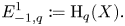
Corollary 4.5 The überhomology groups $\ddot {\mathrm {B}}^j_i (X)$ inherit a further differential

for all $i\geq 0$ and $0\leq j\leq m=V(X)$
 . Hence, $(\ddot {\mathrm {B}}^j_i (X),\, \delta ^{(2)})$
 is a chain complex.
Proof. The differential $\delta ^{(2)}\colon \ddot {\mathrm {B}}^j_i (X)\to \ddot {\mathrm {B}}^{j+2}_{i+1} (X)$ is precisely the differential $\delta ^{(2)}$
 of the second page $E^2_{*,*}$
 of the augmented Mayer–Vietoris spectral sequence.
Note that the induced differential $\delta ^{(2)}$ is related to the connecting homomorphism in the Mayer–Vietoris long exact sequence. Furthermore, the transgression of the augmented Mayer–Vietoris spectral sequence induces a (partially defined) map

where $m=|V(X)|$ and $k=0,\,\dots,\, m-2$
 .
.
As a consequence of theorem 1.1, the next computations of $0$ -degree überhomology groups follow.
Example 4.6 The homology groups $\ddot {\mathrm {B}}^j_i (X)$ of the simplicial complex in example 3.13 are all zero, except for $\ddot {\mathrm {B}}^3_1 (X)$
 and $\ddot {\mathrm {B}}^1_0 (X)$
 , both isomorphic to $\mathbb {Z}$
 . The two classes are paired by the differential $\delta ^{(2)}\colon \ddot {\mathrm {B}}^1_0 (X)\to \ddot {\mathrm {B}}^{3}_{1} (X)$
 , and the bold homology class is paired with the fundamental class of $X$
 . In this case, $\delta ^{(2)}$
 at $\ddot {\mathrm {B}}^1_0 (X)$
 agrees with the transgression $\tau$
 , and is an isomorphism. Consider the square from example 3.14; it has non-trivial homology groups $\ddot {\mathrm {B}}^4_1 (X)$
 and $\ddot {\mathrm {B}}^2_0 (X)$
 ; these are again paired by the differential (the transgression) $\delta ^{(2)}$
 , which is an isomorphism.
Example 4.7 The only non-trivial $0$ -degree überhomology groups of the standard spheres $\partial \Delta ^m$
 of example 3.15 are $\ddot {\mathrm {B}}^{m+1}_{m-1} (\partial \Delta ^m)$
 and $\ddot {\mathrm {B}}^1_0 (\partial \Delta ^m)$
 . Note that, in such case, the bold homology class and the class of $\ddot {\mathrm {B}}^{m+1}_{m-1} (\partial \Delta ^m)$
 are still paired, but by higher differentials in the augmented spectral sequence. However, the transgression map still yields an isomorphism between the groups $\ddot {\mathrm {B}}^{m+1}_{m-1} (\partial \Delta ^m)$
 and $\ddot {\mathrm {B}}^1_0 (\partial \Delta ^m)$
 .
.
Example 4.8 Consider the simplicial complex $X$ obtained from two $2$
 -simplices, glued together along one edge, with vertices as in figure 7. Call $v_0,\, v_3$
 the external vertices and $v_1,\, v_2$
 the vertices of the common edge. Then, the subcomplexes $\mathrm {ast}_X(v_i)$
 and all the possible intersections, except for $\mathrm {ast}_X(v_1)\cap \mathrm {ast}_X(v_2)$
 , are contractible. The subcomplex $\mathrm {ast}_X(v_1)\cap \mathrm {ast}_X(v_2) = \{ v_0,\, v_3\}$
 is disconnected. The spectral sequence converges at the second page, where it is completely trivial. Hence, the homology groups $\ddot {\mathrm {B}}^j_i (X)$
 of $X$
 are all zero.
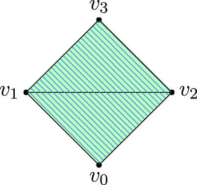
Figure 7. Suspension of the $1$ -simplex.
5. Applications
In this section, we provide some consequences and applications of theorem 1.1. First, we recall the definition of $d$ -Leray complexes.
Definition 5.1 A CW-complex $X$ is $d$
 -Leray if the reduced homology of all induced subcomplexes of $X$
 is trivial for all $i\geq d$
 . A cover $\mathcal {U}$
 of $X$
 is $d$
 -Leray if all its elements are $d$
 -Leray.
Equivalently, by [Reference Kalai and Meshulam33, Proposition 3.1], a simplicial complex $X$ is $d$
 -Leray if $\widetilde {\mathrm {H}}_i(\mathrm {lk}_X(\sigma ))=0$
 for all simplices $\sigma$
 in $X$
 and $i\geq d$
 . The property of being $d$
 -Leray has consequences on the convergence of the Mayer–Vietoris spectral sequence. For example, the following result can be readily deduced from theorem 1.1:
Proposition 5.2 Let $X\neq \Delta ^m$ be a connected, contractible, simplicial complex. If the anti-star cover of $X$
 is $1$
 -Leray, then all the homology groups $\ddot {\mathrm {B}}^j_i (X)$
 are zero.
Proof. If the anti-star cover is $1$ -Leray, then the first page of the augmented Mayer–Vietoris spectral sequence has non-trivial elements only for $q=0$
 . The spectral sequence converges to zero at the second page, since $X$
 is contractible.
This proposition provides a generalization of [Reference Caputi, Celoria and Collari10, Theorem 5.1]: the bold homology of a connected tree with at least three vertices is trivial. Indeed, in this case, the anti-star cover is $1$ -Leray, and the bold homology is the $0$
 -part of $\ddot {\mathrm {B}}^*_* (X)$
 . Another example is given by ‘polygonal neighbourhoods of trees’:
Example 5.3 Let ${\tt T}$ be a tree and choose an abstract full polygon $P$
 (i.e. a $2$
 -cell) on at least $n$
 edges, where $n=\max _{v\in {\tt T}} \deg (v)+2$
 . Then, for each vertex $v$
 of ${\tt T}$
 take a copy $P^v$
 of $P$
 at $v$
 ; for each edge $(v,\,w)$
 , glue $P^v$
 and $P^w$
 along a free face. As in ${\tt T}$
 there are no cycles, the construction yields a contractible CW-complex $X({\tt T})$
 (it is a simplicial complex only when $P$
 is a triangle). Note that the construction may yield different complexes, even for a fixed choice of $P$
 . In any case, the anti-star cover of $X({\tt T})$
 is $1$
 -Leray. Hence, if ${\tt T}\neq \Delta ^1$
 , all the groups $E^2_{*,*}(X({\tt T}))$
 of the associated augmented Mayer–Vietoris spectral sequence are trivial – by the same arguments of proposition 5.2. Consider now the $1$
 -skeleton of $X({\tt T})$
 , which is a connected graph, and has homology in dimension $1$
 of rank $|V({\tt T})|$
 . The anti-star cover associated with such graph is not $1$
 -Leray any more. However, observe that the $(q=0)$
 -row of the augmented Mayer–Vietoris spectral sequence is still trivial (whether the polygons are boundary of $2$
 -cells does not affect the number of connected components, nor the induced $p$
 -differentials). Therefore, the bold homology of polygonal neighbourhoods of trees ($\neq \Delta ^1$
 ) is completely trivial.
Denote by ${\tt I}_m$ the path graph on $m$
 vertices, and by $\square$
 the Cartesian product of graphs.
Corollary 5.4 If $m\geq 3$ , then all graph products ${\tt I}_m\square {\tt I}_2$
 have trivial bold homology.
Proof. Note that the product ${\tt I}_m\square {\tt I}_2$ can be seen as a polygonal neighbourhood of ${\tt I}_m$
 , by choosing the polygon $P$
 to be a square. The product ${\tt I}_m\square {\tt I}_2$
 is not contractible, nor the anti-star cover is $1$
 -Leray. However, the same reasoning as in example 5.3 shows that the graph ${\tt I}_m\square {\tt I}_2$
 has trivial bold homology.
As a consequence, the connected domination polynomial of ${\tt I}_m\square {\tt I}_2$ , evaluated at $-1$
 , is trivial. We point out that, in general, counting connected dominating sets for grids is not straightforward; see also [Reference Goto and Kobayashi24, Reference Srinivasan and Narayanaswamy38].
A priori, one can use properties of the anti-star cover of closed manifolds to deduce properties of their $1$ -skeleton's bold homology. For instance, assume that $M$
 is a closed connected non-orientable $n$
 -manifold. Consider a $m$
 -vertex triangulation $T$
 of $M$
 . If the anti-star cover is $1$
 -Leray, then the first page of the augmented Mayer–Vietoris spectral sequence $E^1_{p,q}$
 is zero for all $p\geq 0$
 and $q\geq 1$
 , whereas $E^{1}_{-1,n-1} = H_{n-1}(M;\mathbb {Z}) \cong \mathbb {Z}_2$
 , see [Reference Hatcher28, Corollary 3.28]. The spectral sequence converges to an acyclic total complex, yielding an isomorphism:
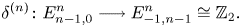
Since $E^2_{n-1,0}\cong E^n_{n-1,0}$ , then $\ddot {\mathrm {B}}^{m}_{n-1}(M;\mathbb {Z})\cong \mathbb {H}^{m-n}(M;\mathbb {Z})\cong \mathbb {Z}_2$
 , and the bold homology would contain torsion. Unfortunately, the anti-star cover of a non-orientable closed connected $n$
 -manifold is $n$
 -Leray. Therefore, we can not infer the existence of torsion classes in bold homology.
Q 5.5 Is it possible to find torsion in the integral bold homology of a simplicial complex?
Given a simple graph ${\tt G}$ , denote by $\operatorname {\mathrm {Fl}}({\tt G})$
 its flag complex, i.e. the simplicial complex whose simplices are given by the complete subgraphs of ${\tt G}$
 . As remarked in [Reference Tancer39, Section 3.2], the only $0$
 -Leray complexes are the standard simplices $\Delta ^n$
 , whereas $1$
 -Leray complexes are flag complexes on chordal graphs. An example of $2$
 -Leray and $3$
 -Leray complexes is given by flag complexes of line graphs of complete bipartite graphs, and complete graphs, respectively [Reference Holmsen and Lee29, Theorem 1.1]. A class generalizing bipartite graphs is given by triangle-free graphs.
Proposition 5.6 Let ${\tt G}$ be a connected triangle-free graph on $m$
 vertices. Then,
(i) $\mathbb {H}^{m}({\tt G};\mathbb {Z})=\mathbb {H}^{m-1}({\tt G};\mathbb {Z})=0$
;(ii) $\mathbb {H}^{m-2}({\tt G};\mathbb {Z})$
and $\ddot {\mathrm {B}}^{m}_1({\tt G};\mathbb {Z})$ are quotients of $\mathrm {H}_1({\tt G};\mathbb {Z})$;(iii) $\mathbb {H}^{j}({\tt G})\cong \ddot {\mathrm {B}}^{j+2}_1({\tt G})$
for all $0\leq j\leq m-2$.


Proof. As ${\tt G}$ is triangle-free, it follows that $\operatorname {\mathrm {Fl}}({\tt G})={\tt G}$
 , and the anti-star cover of $\operatorname {\mathrm {Fl}}({\tt G})={\tt G}$
 is $2$
 -Leray. An inspection of the spectral sequence, together with corollary 4.5, yields short sequences
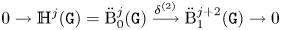
Since the spectral sequence must converge at the third page, $\delta ^{(2)}$ is an isomorphism. The statements follow by theorem 1.1.
In virtue of lemma 2.6, the above proposition implies that the $0$ -degree überhomology of flag complexes on triangle-free graphs is completely determined by their bold homology.
The effect of graph cones on bold homology of graphs was explored in [Reference Caputi, Celoria and Collari10, Proposition 5.3]. Denote by ${\rm Cone}(X)$ the cone of a simplicial complex $X$
 . Recall that, given two chain complexes $(C_*,\,\delta ^C_*)$
 , and $(D_*,\,\delta ^D_*)$
 , and a chain map $\psi : C_* \to D_*$
 the mapping cone of $\psi$
 is the chain complex defined as follows:

The following result is a partial generalization of both [Reference Caputi, Celoria and Collari10, Proposition 5.3] and [Reference Celoria12, Proposition 7.11].
Proposition 5.7 Let $X\neq \Delta ^{m-1}$ be a simplicial complex on $m$
 vertices. Then, there is an isomorphism

of bigraded modules.
Proof. Denote by $v_1,\,\ldots,\,v_m$ the ordered vertices of $X$
 , and by $v_0$
 the coning vertex in ${\rm Cone}(X)$
 . Set $U_i = \mathrm {ast}_X(v_i)$
 , $U'_0 = \mathrm {ast}_{{\rm Cone}(X)}(v_0)$
 , and $U'_i = \mathrm {ast}_{{\rm Cone}(X)}(v_i) \simeq {\rm Cone}(U_i)$
 . Note that all the $U'_i$
 's, as well as their intersections, are non-empty and contractible. Furthermore, $U'_0 = X$
 , and under this identification, each $U_i$
 corresponds to the intersection $U'_0 \cap U'_i$
 . Therefore, we get the isomorphisms

for all $p\geq -1$ and $q$
 , with the conventions that $E^1_{-1,q}(X)=\mathrm {H}_q(X)$
 and $E^1_{-2,q}(X)= 0$
 . We claim that:

where $\phi$ is a graded chain map, $\Delta ^{m-1} = [1,\,\ldots,\,m]$
 , and $\widetilde {C}_p(\Delta ^{m-1})$
 is concentrated in $q$
 -degree $0$
 . To see this, identify the group $\mathrm {H}_0(U'_{i_1}\cap \cdots \cap U'_{i_{p+1}})$
 with the summand in $\widetilde {C}_p(\Delta ^{m-1})$
 spanned by the simplex $[i_1,\,\ldots,\,i_{p+1}]$
 . This identification provides the map $\phi$
 . Since $\widetilde {C}_*(\Delta ^{m-1})$
 is acyclic, the statement follows.
The above reasoning can be extended to suspensions of simplicial complexes:
Theorem 5.8 Let $X$ be a connected simplicial complex on $m$
 vertices, and denote by $\Sigma (X)$
 the suspension of $X$
 . Then, for $q\neq 1$
 the following isomorphisms exist

where $\mathbb {Z}_{(2)}$ indicates a copy of $\mathbb {Z}$
 in überhomological degree $2$
 .
.
Proof. Let $v_1,\,\ldots,\,v_m$ be the vertices of $X$
 and write $\Sigma (X) = X \ast \{ p_1,\,p_2\}$
 . For each $I\subseteq \{ 1\ldots,\,k\}$
 , possibly empty, we shall write $\mathcal {U}_I$
 for the sub-complex of $X$
 spanned by $\{ v_j \}_{j\notin I}$
 . Similarly, given $I\subseteq \{ 1,\,\ldots,\,m\}$
 and $J\subseteq \{1,\,2\}$
 , we denote by $\mathcal {U}_I^{J}$
 the sub-complex of $\Sigma (X)$
 spanned by $\{ v_j \}_{j\notin I}\cup \{ p_r \}_{r\notin J}$
 . Note that there are identifications $\mathcal {U}^{\emptyset }_{I} = \Sigma (\mathcal {U}_I)$
 , $\mathcal {U}^{\{ 1\}}_{I} = \mathcal {U}^{\{ 2\}}_{I} ={\rm Cone} (\mathcal {U}_I)$
 , and $\mathcal {U}^{\{ 1,2\}}_I = \mathcal {U}_I$
 .
.
By definition, the first page of the Mayer–Vietoris spectral sequence decomposes as
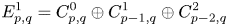
where

For each $q$ , the inclusions $\mathcal {U}_{I \setminus \{ i \}}^{J} \subset \mathcal {U}_{I}^{J}$
 with $J\subseteq \{ 1,\,2\}$
 , induce differentials $\partial _0$
 , $\partial _1$
 , and $\partial _2$
 on $C^{0}_{*,q}$
 , $C^{1}_{*,q}$
 , and $C^{2}_{*,q}$
 , respectively, endowing them with the structure of chain complexes. Similarly, the inclusions $\mathcal {U}_{I}^{J} \subset \mathcal {U}_{I}^{J \setminus \{ j \}}$
 , induce chain maps $\phi _s \colon C^{s}_{*,q} \to C^{s-1}_{*,q}$
 , for $s=1,\,2$
 . The signs of $\phi _1$
 and $\phi _2$
 can be chosen so that the differential on $E^1$
 can be written, with respect to the decomposition in equation (5.1), as follows:

We can thus write $(E^1_{*,q},\, \delta ^{(1)})$ as an iterated cone:

Using the identifications $\mathcal {U}^{\emptyset }_{I} = \Sigma (\mathcal {U}_I)$ , $\mathcal {U}^{\{ 1\}}_{I} = \mathcal {U}^{\{ 2\}}_{I} ={\rm Cone} (U_I)$
 , and $\mathcal {U}^{\{ 1,2\}}_I = \mathcal {U}_I$
 , we can obtain isomorphisms of chain complexes:
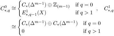
and
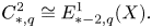
Therefore, for $q=0$ we obtain strong deformation retracts (in the sense of [Reference Bar-Natan6, Definition 4.3]) $C^0_{*,0} \simeq \mathbb {Z}_{(m-1)}$
 and $C^1_{*,0} \simeq 0$
 . In turn (cf. [Reference Bar-Natan6, Lemma 4.5]) these strong deformation retracts induce the following strong deformation retracts:

and thus
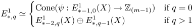
for an appropriate chain map $\psi$ . This proves the statement for $q> 1$
 . Now, if $X^{(1)} \neq {\tt K}_{m}$
 then $\mathbb {H}_1(X^{(1)}) = \ddot {\mathrm {B}}_0^{1}(X)= 0$
 (see [Reference Caputi, Celoria and Collari10, Theorem 1.4]). In fact, we can prove that $E^1_{*,0}(X)$
 (strongly) deformation retracts onto a complex $C_*$
 supported in degrees strictly lower than $m$
 , cf. [Reference Caputi, Celoria and Collari10, Alternative proof of Proposition 4.3]. This implies that

Since $C_*$ is the chain complex whose homology is $\mathbb {H}_{m-*}(X^{(1)}) = \ddot {\rm B}^{m-*}_{0}(X)$
 , the statement follows for $q=0$
 and $X^{(1)} \neq {\tt K}_{m}$
 . Finally, consider the case $X^{(1)} = {\tt K}_{m}$
 . By lemma 2.6, $\mathrm {H}_{m+1}(E^{1}_{*,0}) = \mathbb {H}_{m -* -2}((\Sigma (X))^{(1)})$
 can be computed by considering any simplicial complex $Y$
 such that $Y^{(1)} = (\Sigma (X))^{(1)}$
 . For instance, we can take $Y$
 to be $\Sigma \Delta ^{m-1}$
 . Since $Y$
 is contractible and its anti-star cover is $1$
 -Leray, it follows from proposition 5.2 that $\mathbb {H}_{*}((\Sigma (X))^{(1)}) = 0$
 .
.
Observe that we cannot apply the same reasoning as in the proof of theorem 5.8 for $q>1$ to obtain something about the case $q=1$
 . This is due to the fact that $\mathrm {H}_1(\Sigma X)\neq \mathrm {H}_{0}(X)$
 . We can see also that $\ddot {\mathrm {B}}_{1}^{*}(\Sigma (X))$
 is not necessarily trivial, by taking $X$
 the linear graph with three vertices – cf. example 3.14.
To conclude, we provide the proof of theorem 1.2:
Proof Proof of theorem 1.2
Let $X$ be a finite connected CW-complex and denote by ${\tt G}$
 its $1$
 -skeleton. Since the anti-star cover of $X$
 is $1$
 -Leray, the augmented Mayer–Vietoris spectral sequence converges to the trivial group. Furthermore, the only non-trivial groups in the $E^2$
 -page are in bidegrees $(*,\,0)$
 and $(-1,\,*)$
 . The überhomology groups $\ddot {\mathrm {B}}^j_i (X)$
 are all zero, except for $\ddot {\mathrm {B}}^{m-p-1}_0 (X)\cong \mathrm {H}_p(X)=\ddot {\mathrm {B}}_p^m (X)$
 . The isomorphism between the groups $\ddot {\mathrm {B}}^{m-p-1}_0 (X)$
 and $\ddot {\mathrm {B}}_p^m (X)$
 is given by the transgression. As a consequence, we have

and the statement follows.
Note that the $1$ -Leray assumption in theorem 1.2 is essential. Indeed, consider the simplicial complex of example 3.14 shown in figure 6. The connected domination polynomial of the underlying graph, evaluated at $-1$
 , is $-1$
 , whereas the Euler characteristic of $X$
 is $1$
 .
.
Corollary 1.3 follows immediately from theorem 1.2, after observing that flag complexes of chordal graphs are contractible and $1$ -Leray [Reference Dochtermann and Engström17, Lemma 3.1].
Remark 5.9 Consider the graph ${\tt I}_3\square {\tt I}_2$ . By corollary 5.4, its bold homology is trivial, and $-1$
 is a root of its connected domination polynomial. Hence, the converse of corollary 1.3 does not generally hold, as ${\tt I}_3\square {\tt I}_2$
 is not chordal.
We conclude with a perspective on higher chordality. From [Reference Adiprasito, Nevo and Samper1, Fact 3.1], the anti-star cover $\mathcal {U}^{\mathrm {ast}}$ of a simplicial complex $X$
 is $k$
 -Leray, for $k>1$
 , if and only if $X$
 is resolution $l$
 -chordal for all $l\geq k$
 . Paralleling corollary 1.3, it would be interesting to investigate properties of the connected domination polynomial of the $1$
 -skeleton of such complexes.
Acknowledgements
The authors wish to warmly thank Julius Frank for valuable discussions, and for sharing his code [Reference Frank22]. The authors are also grateful to Dejan Govc, for his comments and feedbacks on the first draft of the paper, and wish to warmly thank the anonymous referees; their comments helped to improve the quality of the paper. The main idea of this paper was born in a bar in Piazza Statuto in Turin. DC was supported by Hodgson-Rubinstein's ARC grant DP190102363 ‘Classical And Quantum Invariants Of Low-Dimensional Manifolds’. CC is supported by the MIUR-PRIN project 2017JZ2SW5.


 Open access