


1. Introduction
Mastering the dynamics of dispersed micro-objects, such as beads, drops or bubbles transported by an external flow, is crucial in many situations, including (i) the control and optimization of two-phase flows through porous materials for the food, pharmaceutical or cosmetic industries (Muschiolik Reference Muschiolik2007; Park, Kim & Kim Reference Park, Kim and Kim2021), (ii) the improvement of heat and mass transfer or the intensification of heterogeneous reactions for energy or chemical applications (Song, Chen & Ismagilov Reference Song, Chen and Ismagilov2006), (iii) the enhanced recovery of residual oils in the petroleum industry (Green & Willhite Reference Green and Willhite1998) and (iv) biomedical and biological applications where these objects represent model systems for cell sorting (Hur et al. Reference Hur, Henderson-MacLennan, McCabe and Di Carlo2011b; Chen et al. Reference Chen, Xue, Zhang, Hu, Jiang and Sun2014).
Nowadays, the emergence of microfluidics that eases manipulation of small objects with the use of a continuous phase, raises new challenges such as object focusing and separation. Different strategies have been developed for continuous flow separation (Pamme Reference Pamme2007). While these techniques appear very different, most of them share the same fundamental principles: the hydrodynamic forces leading to a migration of the objects are modulated either by the geometry of the channels through obstacles, constrictions, expansions or surface textures, or by the external forces acting on the object such as gravitational, electrical, magnetic, centrifugal, optical or acoustical forces. The sources of hydrodynamic forces are twofold: inertial and viscous, as compared by the Reynolds number defined as  $\textit {Re} = \rho _c J d_h / \mu _c$ with $d_h$ the hydraulic diameter of the channel, $J$ the superficial velocity, $\rho _c$ the density of the continuous phase and $\mu _c$ its dynamic viscosity. Microfluidics is generally associated with negligible inertia because of the small characteristic size of the channels. In that case, the hydrodynamic forces are restricted to viscous forces and the linear Stokes equations are used to model the flow (Happel & Brenner Reference Happel and Brenner2012). Nevertheless, an estimation of the Reynolds number for common situations, for instance considering water of viscosity $\mu _c = 1\ {\rm mPa}\ {\rm s}$ and of density $\rho _c = 1000\ {\rm kg}\ {\rm m}^{-3}$ flowing in a channel of diameter $d_h = 100\ \mathrm {\mu }{\rm m}$ with a velocity of $10\ {\rm mm}\ {\rm s}^{-1}$, leads to a value $Re \sim 1$. Thus, the inertial forces are not necessarily negligible and the nonlinear Navier–Stokes equations are often needed to model the flow, especially when an object is transported by the flow (Di Carlo et al. Reference Di Carlo, Irimia, Tompkins and Toner2007).
The nonlinear term of the Navier–Stokes equation which is associated with inertia is of major importance because it breaks the linearity of the Stokes equation and leads to lateral (i.e. cross-stream) motion of dispersed objects evolving in flows with shear gradients (Bretherton Reference Bretherton1962). Segre & Silberberg (Reference Segre and Silberberg1962) observed for the first time such inertial migration for small neutrally buoyant rigid spheres transported in an axisymmetric Poiseuille flow. They noticed that the beads migrate radially to equilibrium positions located at a distance of approximately  $0.3 d_h$ from the cylindrical channel centreline when their diameter $d_d$ is small compared with $d_h$. As a consequence, a randomly distributed suspension of beads focuses onto a narrow equilibrium annulus as it moves downstream the channel (see figure 1a). These observations, unexplained at that time, have drawn the interest of the scientific community. They led to a series of experimental studies on inertial migration in various situations: the case of a non-rotating sphere has been studied by Oliver (Reference Oliver1962), non-neutrally buoyant objects in vertical flow were investigated in various studies (Repetti & Leonard Reference Repetti and Leonard1964; Jeffrey & Pearson Reference Jeffrey and Pearson1965; Karnis, Goldsmith & Mason Reference Karnis, Goldsmith and Mason1966; Aoki, Kurosaki & Anzai Reference Aoki, Kurosaki and Anzai1979) and observations of inertial migration have been extended to different flow geometries such as plane Poiseuille flows (Tachibana Reference Tachibana1973) or more recently flows in rectangular cross-section ducts (Di Carlo et al. Reference Di Carlo, Irimia, Tompkins and Toner2007, Reference Di Carlo, Edd, Humphry, Stone and Toner2009; Hur et al. Reference Hur, Choi, Kwon and Di Carlo2011a; Masaeli et al. Reference Masaeli, Sollier, Amini, Mao, Camacho, Doshi, Mitragotri, Alexeev and Di Carlo2012).

Figure 1. (a) Schematic illustration of the migration of dispersed objects initially randomly distributed across a microchannel. (b) Wall-induced inertial migration force. Streamlines are shown in the laboratory reference frame. (c) Shear-gradient-induced inertial migration force. (d) Deformation-induced migration force for the cases of a drop or a bubble with a viscosity ratio  $\lambda <0.7$ or $\lambda >11.5$. Streamlines are shown in the dispersed object reference frame. Colours in (b–d) show the pressure field differences with a Poiseuille flow: higher in red, lower in blue.
A comprehensive analysis of inertial migration has been obtained by means of analytical models based on the technique of matched asymptotic expansion. In the case of small but finite Reynolds numbers and small bead size compared with the channel diameter, Cox & Brenner (Reference Cox and Brenner1968) derived a scaling for the migration force. Afterwards, Ho & Leal (Reference Ho and Leal1974) provided the spatial evolution of the inertial force along the lateral position in the channel and, by this means, showed that this force changes sign at a distance close to  $0.3d_h$ from the channel centreline. This study highlights that the lateral migration of beads to an equilibrium position results from the interplay between a wall-induced force pointing toward the channel centre and a shear-gradient-induced force oriented toward the channel wall. The wall-induced force develops when a bead is close enough to a wall and arises from the asymmetries of the streamlines and the velocities on either side of the bead, causing a pressure imbalance with a higher pressure on the side near the wall, hence generating a force pointing toward the channel centreline (see figure 1a,b). On the contrary, the shear-gradient-induced force is due to the curvature of the velocity profile and can be understood as follows: because of the non-uniform velocity gradient, the relative velocity of the flow to the bead is higher at the side of larger shear (i.e. close to the wall in a Poiseuille flow) resulting in a smaller pressure at this side. Therefore, the bead moves towards the region of large shear gradient where the magnitude of the relative velocity is the highest (see figure 1a,c). As pointed out by Rivero-Rodríguez & Scheid (Reference Rivero-Rodríguez and Scheid2018a), the equilibrium is reached when the relative velocity of the bead with the mean flow velocity cancels out, namely at the position $\sqrt {2} d_h/4$ from the centreline provided $d_d/d_h \rightarrow 0$. The seminal study of Ho & Leal (Reference Ho and Leal1974) has been extended to the cases of larger Reynolds number (Schonberg & Hinch Reference Schonberg and Hinch1989; Asmolov Reference Asmolov1999) and two-dimensional Poiseuille flows (Hogg Reference Hogg1994), but remains valid only for small bead Reynolds numbers ( $\textit {Re}_d = (d_d/d_h)^2 \textit {Re}$), i.e. in the case of small dispersed objects compared with the channel dimension. According to the investigations of Matas, Morris & Guazzelli (Reference Matas, Morris and Guazzelli2003) and Di Carlo et al. (Reference Di Carlo, Edd, Humphry, Stone and Toner2009), some aspects of inertial migration, such as the impact of the finite size of the dispersed object on its equilibrium position when $d_d/d_h$ gets close to unity, cannot be predicted using these assumptions.
In parallel, experiments on deformable dispersed objects at vanishing Reynolds number, using drops transported in a Poiseuille flow, have shown that the coupling between deformation and the external flow results in a deformation-induced migration force (Goldsmith & Mason Reference Goldsmith and Mason1962). In this situation, the deformability of the dispersed object is quantified by the capillary number  $Ca = \mu _c J /\gamma$ that compares viscous with capillary forces, with $\gamma$ the interfacial tension.
Similarly to Ho & Leal (Reference Ho and Leal1974), Chan & Leal (Reference Chan and Leal1979) used a matched asymptotic expansion method to derive an analytic expression of this deformation-induced migration force. Their study reveals that the orientation of the force strongly depends on the viscosity ratio  $\lambda = \mu _d/\mu _c$, with $\mu _d$ the viscosity of the dispersed phase. In a cylindrical Poiseuille flow, the force points toward the wall for $0.7 \lesssim \lambda \lesssim 10$, while it points toward the channel centreline for $\lambda \lesssim 0.7$ and $\lambda \gtrsim 10$ (see figure 1d). However, their theory is accompanied by inherent limiting hypotheses such as small drop deformations, small drop diameters compared with the channel dimension and $\lambda < 1/Ca$. Moreover, it is also important to note that the wall effects that push deformed drops toward the channel centreline were neglected (Kennedy, Pozrikidis & Skalak Reference Kennedy, Pozrikidis and Skalak1994). Coulliette & Pozrikidis (Reference Coulliette and Pozrikidis1998) used numerical simulations based on boundary integral methods to study the case of deformation-induced migration of drops in a Stokes flow (i.e. inertialess flow) with a viscosity ratio $\lambda =1$. By this means, the authors investigated the case of large deformations and studied the impact of the drop diameter $d_d$ on the capillary migration processes. They showed that, in all cases, after an initial period of rapid deformation, the drops migrate radially toward the centreline.
The first study dealing with deformable dispersed objects at finite Reynolds number gathering inertial- and deformation-induced migration forces was led by Mortazavi & Tryggvason (Reference Mortazavi and Tryggvason2000). To investigate the dynamics of drops in Poiseuille flow for few values of the capillary number, Reynolds number, viscosity ratio and drop diameter, they used two-dimensional, supplemented with a few three-dimensional, numerical simulations based on the finite element method coupled with locally adaptive moving mesh. They have shown that large drops with  $d_d \approx d_h$ always move toward the channel centreline. For smaller drops and intermediate Reynolds numbers (i.e. $\textit {Re} = [5\unicode{x2013}50]$), the competition between inertial- and deformation-induced forces leads to the migration toward an off-centred equilibrium position. This equilibrium position gets slightly closer to the wall when increasing the Reynolds number while keeping constant the Weber number $We=Re\,Ca$, which compares inertial with capillary forces. On the contrary, increasing the drop viscosity or the drop deformation (by increasing the Weber number) has the opposite effect. They also reported that, for large Reynolds number and/or small viscosity ratio, the equilibrium position is reached after transient oscillations around the steady state. Moreover, above a critical Reynolds number and/or below a critical viscosity ratio, oscillations are not damped anymore and no equilibrium position is observed.
Later, Chen et al. (Reference Chen, Xue, Zhang, Hu, Jiang and Sun2014) carried out three-dimensional (3-D) transient simulations and experiments with deformable drops in rectangular cross-section channels of a width larger than the height. In this channel geometry, they have shown that drops migrate to the centreline in the height direction and to two equilibrium positions in the width direction. Moreover, in agreement with the study of Mortazavi & Tryggvason (Reference Mortazavi and Tryggvason2000), the authors reported that, increasing the drop deformation by increasing the Weber number, displaces the equilibrium positions closer to the channel centreline.
More recently, also using numerical simulations based on the finite element method, Rivero-Rodríguez & Scheid (Reference Rivero-Rodríguez and Scheid2018a) solved the full steady Navier–Stokes equations to provide a detailed study on the dynamics of dispersed objects depending on the inertial and capillary migration forces for the case of bubbles. The authors realized a systematic exploration of the influence of the bubble size, Reynolds and capillary numbers on the velocity and the lateral position for these objects, and this for two boundary conditions at the bubbles’ interface: stress free and no slip, in order to consider the effect of the interface rigidity in two extreme cases, namely for a perfectly clean and deformable bubble, and for a rigid bubble when involving surfactants or dust, for instance (equivalently to the rigid bead case), respectively.
Although these works give insights into the dynamics of dispersed objects transported by an external flow in a microchannel subject to inertial and/or capillary forces, they focused on specific dispersed objects, some limiting cases or a few sets of parameters. In the present study, we aim to offer a general vision of this problem by performing, both experimentally and numerically, a systematic study of the influence of all parameters of the problem (Reynolds and capillary numbers, dispersed object diameter, density ratio and viscosity ratio) on the equilibrium velocity and position of the dispersed objects, and this over a wide range of parameters. With this intention, we explore the dynamics of various dispersed objects, such as beads, bubbles and drops, in various regimes, which enables us to highlight the sole and combined roles of inertia and capillary effects on lateral migration and its impact on the object velocity.
The structure of the article is as follows. We first present, in § 2, the experimental set-up and methods we used to characterize the equilibrium velocity and lateral position of these various dispersed objects (beads, drops and bubbles) in a cylindrical microchannel. In § 3, we describe a steady 3-D Navier–Stokes model for incompressible two-phase fluids including both the effects of inertia and potential interfacial deformations of the dispersed objects. Two reduced versions of the model are then proposed to specifically and easily compute the equilibrium velocity of the dispersed objects or the stability of their equilibrium centred positions. In § 4, we first compare the experimental results with the numerically determined ones and then use the numerical models to extend our understanding of the dynamics of dispersed objects over a larger range of parameters. Moreover, we propose a useful correlation for the equilibrium velocity of the dispersed objects as functions of its diameter, position and viscosity ratio, and we discuss the influence of the Reynolds number, capillary number, viscosity ratio and density ratio on the stability of their equilibrium centred positions. Finally, conclusions are presented in § 5.
2. Experimental set-up and methods
The experiments consist of characterizing the stationary dynamics of a dispersed micro-object, such as a bead, a bubble or a drop, transported by an external flow within a cylindrical microchannel. A schematic of the experimental set-up is provided in figure 2.
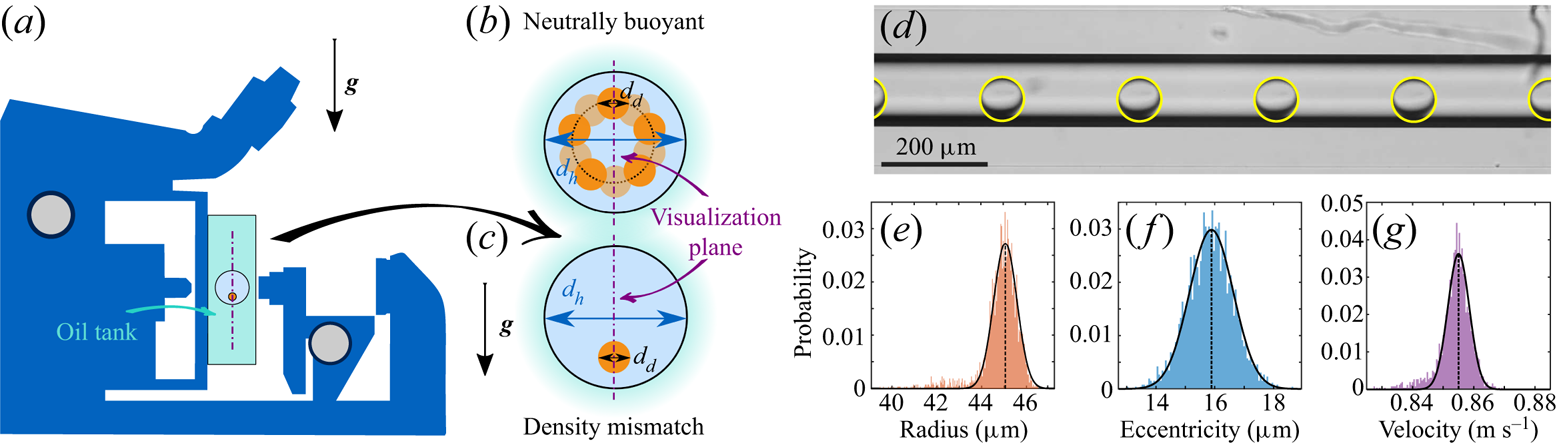
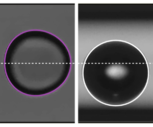
Figure 2. (a) Schematic illustration of the experimental set-up involving an inverted microscope flipped at  $90^\circ$ to observe the dynamics of dispersed objects transported by an external flow within a microcapillary. (b–c) Cross-section of the microcapillary. If migration occurs, while a neutrally buoyant object would migrate toward an annulus of equilibrium, a density mismatch between the two phases results in a migration occurring exclusively along the gravitational axis. The latter scheme corresponds to the case where the object is denser than the continuous phase. (d) Typical experimental images showing a drop of FC-770 transported from left to right in water at different times ( $d_h = 153 \pm 3\ \mathrm {\mu }{\rm m}$, $\textit {Re} = 87$, ${Ca}= 1.3 \times 10^{-3}$, see table 1 for additional information). A downward migration is observed here due to inertial effects. (e–g) Distributions of the drop radius, eccentricity and velocity resulting from the image analysis of the experiment presented in (d), in which the vertical dotted lines correspond to the averaged values.
2.1. Experimental apparatus and image analysis
Two-phase flows are generated and flow within a horizontal glass microcapillary (Postnova Analytics). The flow rate of the continuous liquid phase is imposed using a high precision syringe pump (Nemesys, Cetoni), and a flow meter (Coriolis M12, Bronkhorst) is used in series to verify that it reaches its setpoint. The flow rate of the dispersed phase is controlled using either a pressure controller (MFCS-EX, Fluigent) for experiments involving bubbles, or a second syringe pump (Nemesys, Cetoni) coupled with a flow meter (Flow unit, Fluigent) when drops are investigated. Note that microcapillaries of different inner diameters  $d_h$ have been used depending on the type of dispersed micro-object involved in the experiments: $d_h = 52 \pm 1\ \mathrm {\mu }{\rm m}$ or $59 \pm 1 \ \mathrm {\mu }{\rm m}$ with beads and $d_h = 153 \pm 3\ \mathrm {\mu }{\rm m}$ or $188 \pm 1\ \mathrm {\mu }{\rm m}$ with drops and bubbles. These values have been measured using an optical profilometer (Keyence VK-X200 series).
The dynamics of the micro-objects is observed using an inverted microscope (Nikon Eclipse-Ti) equipped with a 10X TU Plan Fluor objective and images are recorded with a high-speed camera (IDT Y3 Motionpro) at a rate of  $3030\ {\rm frames}\ {\rm s}^{-1}$. To ensure a precise observation of the dispersed micro-objects, we first limit image deformations caused by optical refraction effects by placing the microcapillary within a glass tank filled with light mineral oil (Sigma Aldrich), whose refractive index ( ${n_{{oil}}} = 1.467$) is very close to that of glass ( ${n_{glass}} =1.470$). Second, we take advantage of gravity by turning the microscope by $90^{\circ }$ to force the dispersed micro-objects, whose density slightly mismatches the density of the continuous phase, to always stay in the visualization plane parallel to the gravitational axis and passing through the channel centre. This trick makes the equilibrium position unique, as illustrated in figures 2(b) and 2(c). The dynamics of the transported dispersed objects is recorded at a distance of few tens of centimetres from the capillary inlet in order to ensure a quasi-steady regime to be achieved. A typical experimental visualization is shown in figure 2(d). Note that this image actually corresponds to the superposition of raw images recorded at six consecutive times and hence shows the same moving object (a drop here) at six different positions in the field of view of the camera.
Then, a classical image processing, based on binarization and standard Hough's transform (using ImageJ (Schneider, Rasband & Eliceiri Reference Schneider, Rasband and Eliceiri2012) and Matlab routines), is performed to fit the dispersed object shape over time and extract its radius  $d_d/2$, as well as its equilibrium velocity $V$ and eccentricity $\varepsilon _d$ (i.e. the transverse distance of the object centre from the microchannel centreline). Note that, since in a recorded movie we are able to follow the dynamics of numerous dispersed objects and because experiments are repeated several times, a statistical measurement of these quantities is obtained, from which we derive their mean values (see figure 2e–g). Typical standard deviation on the eccentricity distribution corresponds to the size of one pixel ( $1.085\ \mathrm {\mu }{\rm m}$) and thus on the resolution of our images. The radius distribution is even narrower, the standard deviation corresponding to half a pixel, highlighting the high monodispersity of the dispersed objects generated. The standard deviation on the velocity distribution corresponds to variations of the distance travelled by the object between two consecutive images and is of the order of one to two pixels divided by the time interval between consecutive frames ( $0.7\ {\rm mm}\ {\rm s}^{-1}$).
2.2. Continuous and dispersed phases
In order to vary the viscosity ratio of the dispersed phase to the continuous phase  ${\lambda = \mu _d/\mu _c}$, we consider different micro-objects for the dispersed phase, such as beads ( ${\lambda \to \infty}$), bubbles ( $\lambda \to 0$) and drops (intermediate $\lambda$), and various liquids for the continuous phase.
As non-deformable objects, we used rigid, monodispersed and spherical polystyrene beads (Microbeads AS) suspended in a solution of water containing 7 % of NaOH salt in order to almost match the density of the continuous phase with that of the polystyrene beads. To additionally vary the size of this dispersed object, we experimented with beads of various diameters from  $d_d=10$ to $50\ \mathrm {\mu }{\rm m}$.
As deformable objects, we considered bubbles and drops generated using the Raydrop device (Secoya Technologies), a drop generator based on a non-embedded co-flow-focusing technology, ensuring the generation of drops or bubbles at high frequency with a very good reproducibility (Dewandre et al. Reference Dewandre, Rivero-Rodríguez, Vitry, Sobac and Scheid2020). The versatility of this tool enables the use of different couples of fluids and an excellent control of the drops or bubbles sizes. Note that, to vary the size of these dispersed objects, we use different strategies depending on their nature. For drops, we impose a constant flow rate for the dispersed phase and vary the one of the continuous phase, while, for bubbles, we use a constant flow rate for the continuous phase and we vary the inlet pressure of the dispersed phase.
Table 1 summarizes all beads and fluids employed for the continuous and dispersed phases together with the corresponding ratios of viscosities  $\lambda$ and densities $\varphi = \rho _d/\rho _c$, and the ranges of dimensionless diameters $d=d_d/d_h$, Reynolds number $Re$ and capillary number $Ca$ encountered in our experiments. For convenience, our results are sometimes represented as functions of the Laplace number $La=Re / Ca$, that relates the inertial and capillary forces to the viscous forces, and of the Weber number $We=Re\,Ca$, which describes the competition between inertial forces and capillary forces.
Table 1. Summary of the different situations experimentally investigated in this work.

3. Modelling
The experimental study is complemented by numerical simulations that model the dynamics of dispersed micro-objects (i.e. beads, bubbles or drops) transported by an external flow in a cylindrical channel for Reynolds number ranging from low to intermediate values. More specifically, we model the dynamics of a steady train of equally spaced dispersed objects in a cylindrical microchannel. Thus, the present modelling can actually be considered as a generalization of the one presented in Rivero-Rodríguez & Scheid (Reference Rivero-Rodríguez and Scheid2018a), dedicated to the bubbles and beads cases (i.e. in the limit cases  $\lambda \to 0$ and $\lambda \to \infty$, respectively), to drops (i.e. for all $\lambda$) by considering the internal flow within the dispersed objects.
As previously mentioned, different equilibrium positions are possible depending on the size of the dispersed object and on the balance of the involved forces such as viscous, inertial, capillary and body ones, as due to gravity or magnetic fields.
To model this situation, we consider a volume  $\mathcal {V}$ containing one dispersed object of volume $\mathcal {V}_d$ and of equivalent diameter $d_d = ({6 \mathcal {V}_d/{\rm \pi} })^{1/3}$, delimited by the walls of the channel, $\varSigma _W$, two cross-sections of the channel, $\varSigma _{in}$ and $\varSigma _{out}$, and the dispersed object surface, $\varSigma _d$, as schematized in figure 3. The continuous phase has a density $\rho _c$ and a viscosity $\mu _c$, whereas the dispersed phase has a density $\rho _d$ and a viscosity $\mu _d$. It is assumed that the system is isothermal and the evolution of the dispersed object can be considered as quasi-steady in the absence of either vortex shedding or turbulence.
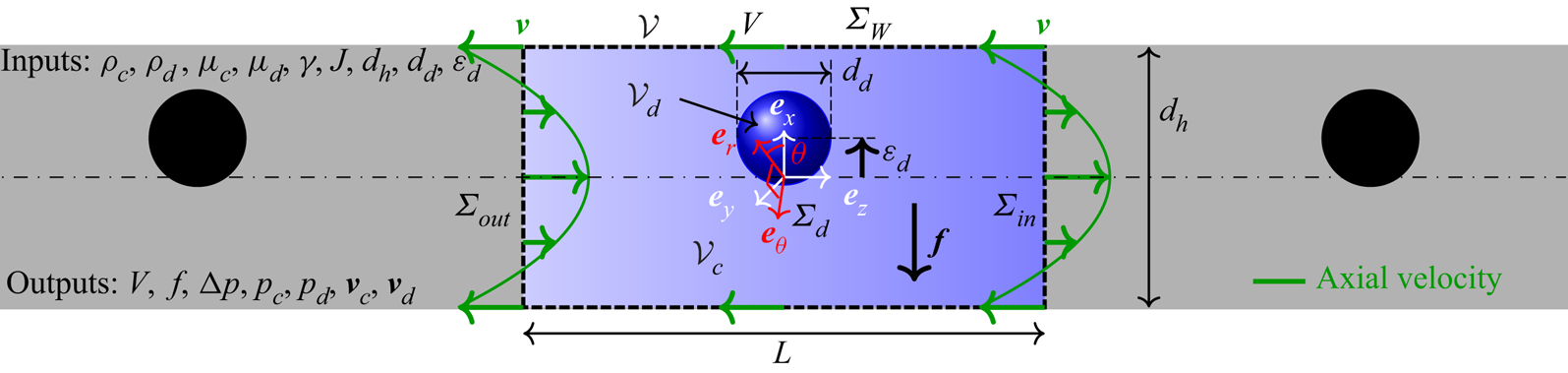
Figure 3. Sketch of the modelled segment of a train of equally spaced dispersed objects in a circular microchannel and definition of the coordinate systems and geometrical parameters.
We include interfacial tension  $\gamma$ and a uniform body force $\boldsymbol {f}$ exerted on the continuous phase in the transverse direction. Gravity is neglected since the radial component of this force is negligible in the experiments as the Froude number that compares the gravitational with the inertial forces, ${Fr}=\sqrt {J^2 \rho _c/(|\rho _c-\rho _d|gd_h)}$, where $g$ in the gravitational acceleration, is always large ( ${Fr}\gg 1$) due to the small channel size and the large flow velocities. In the azimuthal direction there is no component of either inertial- or deformation-induced migration, hence dispersed objects are in equilibrium where the contribution of gravity vanishes, namely in the radial direction that aligns with gravity, leading to one stable equilibrium position.
The two phases flow inside a cylindrical channel of diameter  $d_h$ with a mean velocity $J$, producing a pressure drop due to the Poiseuille flow modified by the presence of a dispersed object, $\Delta p$, along a segment of length $L$. The dispersed object travels with a velocity $V$ at a transverse equilibrium position $\boldsymbol {\varepsilon }$ measured from the centre of the channel which coincides with a specific force balance acting on the surface of the dispersed object in the transverse direction. Periodic boundary conditions are considered without loss of generality between the $\varSigma _{in}$ and $\varSigma _{out}$ cross-sections such as $L$ becomes the spatial periodicity of a train of dispersed object, yet taken large enough to avoid interactions between consecutive objects. An upstream velocity $V$ is imposed at the wall of the channel such that the frame of reference is moving with the dispersed object, whose velocity is determined by balancing the forces acting on the dispersed object surface in the streamwise direction. We make use of either Cartesian or cylindrical coordinates depending on the needs. Note that, although in the present study we consider only small dispersed objects with $d_d/d_h < 1$, there is no size limitation in the described model.
In what follows, we first present a general model, based on a steady three-dimensional isothermal two-phase flow modelling including the effect of inertia and the deformability of the interphase, and composed by (3.2)–(3.6). Then, the general model is conveniently simplified yielding to two reduced and independent models, enabling us to specifically compute: (i) the velocity of the dispersed object in the inertialess and non-deformable limit and (ii) the stability of the centred position using a linear perturbation and expansion in its lateral position around the axisymmetric solution. These two reduced models offer the advantages of a gain both in physical understanding and in computation time, the latter enabling us to provide an exhaustive parametric analysis.
It is worth mentioning that the equations of the models are presented in dimensionless form. To do so, the characteristic length, velocity and pressure are taken as the diameter of the channel  $d_h$, the superficial velocity $J$ and the viscous stress $\mu _c J / d_h$. The dimensionless numbers of the problem are
 \begin{equation} {Ca}=\frac{\mu_c J }{\gamma} , \quad \textit{Re}=\frac{\rho_c J d_h }{\mu_c} , \quad \lambda=\frac{\mu_d}{\mu_c} , \quad \varphi=\frac{\rho_d}{\rho_c} , \quad d = \frac{d_d}{d_h} , \quad \varepsilon = \frac{\varepsilon_d}{d_h}. \end{equation}
In addition, the Laplace number  ${La}=\textit {Re} / {Ca}$ and the Weber number ${We}=Re\,Ca$ will also be used for representing the results.
3.1. Equations of the general model
The flow of both phases in the modelled segment of the channel can be analysed by solving, in the reference frame attached to the dispersed object, the steady and dimensionless Navier–Stokes equations for incompressible fluids
 \begin{equation} \boldsymbol{\nabla} \boldsymbol{\cdot} \boldsymbol{v}_i = 0, \quad \varphi_i \textit{Re} \left(\boldsymbol{v}_i \boldsymbol{\cdot} \boldsymbol{\nabla} \right) \boldsymbol{v}_i = \boldsymbol{\nabla} \boldsymbol{\cdot} \boldsymbol{\mathsf{T}}_{i} , \quad \mbox{in } \mathcal{V}_i , \end{equation}
with  $\boldsymbol{\mathsf{T}}_{i} = -\boldsymbol {\nabla } p_i + \lambda _i [ \boldsymbol {\nabla } \boldsymbol {v}_i + (\boldsymbol {\nabla } \boldsymbol {v}_i)^{\rm T}]$, $p_i$ and $\boldsymbol {v}_i = (u_i, v_i, w_i)$ being the dimensionless stress tensor, reduced pressure and velocity vector, respectively. The subscript $i$ may refer to continuous $c$ or dispersed $d$ phases with $\lambda _c=1$, $\lambda _d=\lambda$, $\varphi _c=1$ and $\varphi _d=\varphi$. For the sake of compactness, the subscript $i$ will be omitted when referring to any of both phases and made explicit when referring to only one of them.
Since the difference between the variables in both phases appears in the equations at the level of the interface, we introduce the double brackets operator defined as  $[\kern-1pt[ \star ]\kern-1pt] = \star _c - \star _d$. The impermeability condition, continuity of velocity and stress jump together with the Young–Laplace equation write
 \begin{equation}
\boldsymbol{v}_c
\boldsymbol{\cdot} \boldsymbol{n}=\boldsymbol{0} , \quad
[\kern-1pt[ \boldsymbol{v} ]\kern-1pt]=0 , \quad [\kern-1pt[
\boldsymbol{\mathsf{T}} ]\kern-1pt] \boldsymbol{\cdot}
\boldsymbol{n}= \boldsymbol{D}_s {Ca}^{{-}1} + \boldsymbol{f}
\boldsymbol{\cdot}
(\boldsymbol{x}-\boldsymbol{\varepsilon}) \boldsymbol{n} ,
\quad \mbox{at } \varSigma_{d} ,
\end{equation}
\begin{equation}
\boldsymbol{v}_c
\boldsymbol{\cdot} \boldsymbol{n}=\boldsymbol{0} , \quad
[\kern-1pt[ \boldsymbol{v} ]\kern-1pt]=0 , \quad [\kern-1pt[
\boldsymbol{\mathsf{T}} ]\kern-1pt] \boldsymbol{\cdot}
\boldsymbol{n}= \boldsymbol{D}_s {Ca}^{{-}1} + \boldsymbol{f}
\boldsymbol{\cdot}
(\boldsymbol{x}-\boldsymbol{\varepsilon}) \boldsymbol{n} ,
\quad \mbox{at } \varSigma_{d} ,
\end{equation}
where  $\boldsymbol {x}$ is the position vector, $\boldsymbol {n}$ is the outer normal to the continuous domain, $\boldsymbol {f}$ is the body force and $\boldsymbol{D}_s \star = \boldsymbol {\nabla } \boldsymbol{\cdot} \boldsymbol{\mathsf{I}}_s \star$ is the intrinsic surface derivative previously introduced in Rivero-Rodríguez & Scheid (Reference Rivero-Rodríguez and Scheid2018a), with $\boldsymbol{\mathsf{I}}_s=\boldsymbol{\mathsf{I}} - \boldsymbol {n} \boldsymbol {n}$ the surface identity tensor, which is independent of the orientation of $\boldsymbol {n}$.
It is worth relating the body force and the migration force, defined as the hydrodynamic force exerted on the dispersed phase by the continuous phase,  $-\int _{\varSigma _d} \boldsymbol{\mathsf{T}}_c \boldsymbol{\cdot} \boldsymbol {n} \,{\rm {d}} \varSigma$. To do so, (3.3c) is integrated among $\varSigma _d$, leading to $-\int _{\varSigma _d} \boldsymbol{\mathsf{T}}_c \boldsymbol{\cdot} \boldsymbol {n} \,{\rm {d}} \varSigma = \boldsymbol {f} \mathcal {V}_d$, where it has been taken into account that (i) the surface tension does not contribute in the force balance, $\int _{\varSigma _d} \boldsymbol{D}_s {Ca}^{-1} \,{\rm {d}} \varSigma = \boldsymbol {0}$, and (ii) that the dispersed phase is in equilibrium, i.e. the total force exerted on the dispersed phase by the continuous phase vanishes, $\int _{\varSigma _d} \boldsymbol{\mathsf{T}}_d \boldsymbol{\cdot} (-\boldsymbol {n}) \,{\rm {d}} \varSigma = \boldsymbol {0}$, as it can be inferred by integrating (3.2) for $i=d$ over $\mathcal {V}_d$. For this reason, $\boldsymbol {f}$ is referred hereafter as either external body force or migration force (per unit volume), indistinctly.
The velocity field and the reduced pressure gradient are periodic along a distance  $L$, producing a pressure drop $\Delta p$
 \begin{equation} \boldsymbol{v} \left(\boldsymbol{x}\right)=\boldsymbol{v} \left(\boldsymbol{x} + L \boldsymbol{e}_z \right) , \quad \partial_z \boldsymbol{v} \left(\boldsymbol{x}\right)= \partial_z \boldsymbol{v} \left(\boldsymbol{x} + L \boldsymbol{e}_z\right) , \quad p \left(\boldsymbol{x}\right) = p \left(\boldsymbol{x} + L \boldsymbol{e}_z\right) + \Delta p , \end{equation}
which must be imposed at any position in  $\varSigma _{out}$. In the reference frame attached to the dispersed object moving at the equilibrium velocity $V$, the velocity of the liquid at the wall writes
 \begin{equation} \boldsymbol{v}_c ={-}V \boldsymbol{e}_z \quad \mbox{at } \varSigma_W . \end{equation}
 Both domains have impermeable boundaries, as shown in (3.3a,b) and (3.5), thus requiring us to impose a pressure reference at one point for each phase. One pressure represents the absolute pressure reference which is set to 0, i.e.  $p_c=0$, at one point arbitrarily chosen in $\boldsymbol {x} \in \mathcal {V}_c$, whereas the other one remains to be determined, i.e. $p_d=p_{{ref}}$, at one point arbitrarily chosen in $\boldsymbol {x} \in \mathcal {V}_d$. Note that $p_{{ref}}$ is an integration constant that is determined below by a volume integral constraint.
Finally, the volume of the drop, centroid position, average flow rate through any cross-section  $\varSigma _{cross}$ and null drag exerted on the object are also imposed
 \begin{align} \int_{\mathcal{V}_d} {\rm{d}} \mathcal{V} = \mathcal{V}_d , \quad \int_{\mathcal{V}_d} \boldsymbol{x} {\rm{d}} \mathcal{V} = \mathcal{V}_d \boldsymbol{\varepsilon} , \quad \int_{\varSigma_{cross}} \left(\boldsymbol{v}_c \boldsymbol{\cdot} \boldsymbol{e}_z + V - 1\right) {\rm{d}} \varSigma =0 , \quad \boldsymbol{f} \boldsymbol{\cdot} \boldsymbol{e}_z = 0 , \end{align}
which determine the values of the variables  $p_{ref}$, $\boldsymbol {f}$, $\Delta p$ and $V$, respectively.
Respecting the symmetry, the Cartesian coordinate system can be oriented with the vector  $\boldsymbol {e}_x$ aligned with the lateral eccentricity $\boldsymbol {\varepsilon }$ and $\boldsymbol {f}$. Therefore, these vectors can be written as $\boldsymbol {\varepsilon }=\varepsilon \boldsymbol {e}_x$ and $\boldsymbol {f}=f \boldsymbol {e}_x$, where (3.6d) has already been considered.
From the solution of the general model, composed of the system of (3.2)–(3.6), it can be observed that migration forces are induced when either inertia, quantified by the Reynolds number  $\textit {Re}$, or deformability of the interphase induced by the viscous forces, quantified by the capillary number ${Ca}$, are taken into account. Asymptotic expansion of this system of equations in terms of $\textit {Re}$ and ${Ca}$ leads to the following expansion of $V$ and $f$:
$f$:
 $$\begin{gather} V \left(\lambda, d,\varepsilon,\textit{Re},{Ca} \right) = V_0 \left(\lambda, d,\varepsilon \right) + {O}(\textit{Re}^2, \textit{Re} \, {Ca}, {Ca}^2), \end{gather}$$
 $$\begin{gather}f \left(\lambda,d,\varepsilon,\textit{Re},{Ca} \right) = f_{1,\textit{Re}} \left(\lambda, d,\varepsilon \right) \textit{Re} + f_{1,{Ca}} (\lambda, d,\varepsilon) {Ca} + {O}(\textit{Re}^3, \textit{Re}^2\, {Ca}, \textit{Re} \,{Ca}^2, {Ca}^3) , \end{gather}$$
where vanishing terms have been removed, according to the results in Rivero-Rodríguez & Scheid (Reference Rivero-Rodríguez and Scheid2018a), based on the reversibility of the flow. It is observed that for sufficiently small values of  $\textit {Re}$ and ${Ca}$, the velocity of the dispersed object is independent of these numbers, whereas the migration force is proportional to these numbers, vanishing only when both numbers vanish, $\textit {Re}={Ca}=0$, for any arbitrary lateral position of the dispersed object.
Then, several regimes can be classified with respect to the dimensionless numbers as sketched in figure 4. For  $\textit {Re}={Ca}=0$, the system is in the inertialess and non-deformable limit. For non-zero but small values, the migration force is proportional to $\textit {Re}$ and/or ${Ca}$, and we refer to as the linear regime. For sufficiently large values, nonlinearities arise. Analogous regimes can be considered for ${La}=0$ or ${La} \rightarrow \infty$, which represent inertialess or non-deformable systems, respectively, and the nonlinearity of the regime is gauged by ${Ca}$ or $\textit {Re}$.

Figure 4. The considered flow regimes involving inertial and capillary migrations. The bricks and dots represent linear and nonlinear regimes, respectively. The  $\textit {Re}={Ca}=0$ limit is exclusively used in this study for the computation of the velocity of the dispersed objects.
Solving the general model to derive the equilibrium velocity and lateral position of dispersed objects is time and resource consuming because of the numbers of parameters ( $d$,
$d$,  $\lambda$, ${Ca}$, $\textit {Re}$ and $\varphi$) and the tri-dimensionality of the problem. Therefore, in the following, the general model is not used as is, but rather aptly developed and reduced in two different limits, namely, the inertialess and non-deformable limit, mainly used for predicting the equilibrium velocity of the dispersed objects, and the limit case of axisymmetric solutions, to address the question of the stability of their centred position.
3.2. Inertialess and/or non-deformable limit(s)
The system of equations (3.2)–(3.6) allows two non-exclusive limits, namely, inertialess for  $\textit {Re}=0$ and non-deformable for ${Ca}=0$. The inertialess limit can be obtained by substituting $\textit {Re}=0$ in the equations, whereas the non-deformable limit requires more modifications than simply substituting ${Ca}=0$ in the system. In the latter limit, the variations of the curvature with respect to the non-deformable dispersed object for large interfacial tensions are inversely proportional to interfacial tension, leading to a finite pressure $p_s$ irrespective of the value of Ca, provided it is sufficiently small. Thus, the interfacial tension term in (3.3c) is of the form $p_s \boldsymbol {n}$ leading to
 \begin{equation} [\kern-1pt[ \boldsymbol{\mathsf{T}} ]\kern-1pt] \boldsymbol{\cdot} \boldsymbol{n}={-}p_s \boldsymbol{n} + \boldsymbol{f} \boldsymbol{\cdot} (\boldsymbol{x}-\boldsymbol{\varepsilon}) \boldsymbol{n} . \end{equation}
Furthermore, since the interphase deformation vanishes for  ${Ca} = 0$, equations (3.6a,b) no longer hold, the volume and position of the object being a priori imposed. Instead, it must be considered that the overall surface pressure forces applied on a closed surface must vanish, namely
 \begin{equation} \int_{\varSigma_{d}} p_s \boldsymbol{n} \,{\rm{d}} \varSigma =0 . \end{equation}
This model simplification is analogous to that rigorously developed in Rivero-Rodríguez & Scheid (Reference Rivero-Rodríguez and Scheid2018a) in terms of asymptotic expansion in  ${Ca}$ around ${Ca}=0$.
In the inertialess and non-deformable limit, the general model is simplified by combining all modifications explained above for the two non-exclusive limits. Thus, this simplified model reduces to the system of equations (3.2)–(3.3b), (3.8), (3.4a–c)–(3.5), (3.9), (3.6c,d), in which  $\textit {Re}=0$ and ${Ca}=0$. It is worth mentioning that, despite the absence of migration forces in this inertialess and non-deformable limit, the prediction from this simplified model for the dispersed object velocity remains valid over a relatively larger range of values of $\textit {Re}$ and ${Ca}$ in the linear regimes, as observed in (3.7a) since the first-order correction vanishes, and as shown later in § 4.2.2.
3.3. Linear stability of axisymmetric solutions
The equilibrium eccentricity of a dispersed object is analysed here via the determination of the stability threshold of its centred position (i.e.  $\varepsilon =0$), hence considering a neutrally buoyant object (i.e. $f=0$). To do this, the general model (3.2)–(3.6) is perturbed up to first order in eccentricity $\varepsilon$ around $\varepsilon =0$. Thus, $f(\varepsilon )= f_0 + f_1 \varepsilon + {O}(\varepsilon ^2)$, matching the Taylor expansion $f(\varepsilon ) = f\vert _{\varepsilon =0} + \partial f / \partial \varepsilon \vert _{\varepsilon =0} \,\varepsilon + {O}(\varepsilon ^2)$, should reveal from the sign of $f_1 = \partial f / \partial \varepsilon \vert _{\varepsilon =0}$, the stable or unstable character of the centred position. If $f_1<0$, the body force acts in the opposite direction of the lateral displacement and the centred position is stable, while if $f_1>0$, the centred position is unstable and the body force leads to the lateral migration of the dispersed object. Compared with the previous analysis of the position stability based on the prediction of the pitchfork bifurcation when $\partial f / \partial \varepsilon = 0$ (see Rivero-Rodríguez & Scheid (Reference Rivero-Rodríguez and Scheid2018a) in the case of bubbles and beads), this alternative method has the advantage of reducing both the dimensionality of the problem from three-dimensional to axisymmetric two-dimensional and the parametric space, thus requiring much less computational effort and enabling extended parametric analysis on the equilibrium eccentricity.
To proceed, we perturb the axisymmetric geometry which undergoes a displacement of the dispersed object interphase  $\boldsymbol {\delta }= \delta \boldsymbol {n}$. Then, we seek an expansion of the variables in terms of $\varepsilon$ and an analytical $\theta$-dependence in cylindrical coordinates
 $$\begin{gather} p_i \left(r, \theta, z\right)=p_{i0}(r,z) + \varepsilon {\rm e}^{{\rm i}\theta} p_{i1}\left(r,z\right) + {O}(\varepsilon^2) \quad {\mbox{in }}\mathcal{V}_{i0} , \end{gather}$$
 $$\begin{gather}\boldsymbol{v}_i\left(r, \theta, z\right)=\boldsymbol{v}_{i0}\left(r,z,\theta\right) + \varepsilon {\rm e}^{{\rm i}\theta} \, \boldsymbol{v}_{i1}(r,z,\theta) + {O}(\varepsilon^2) \quad {\mbox{in }} \mathcal{V}_{i0} , \end{gather}$$
 $$\begin{gather}\delta\left(r, \theta, z\right) = \varepsilon {\rm e}^{{\rm i}\theta} \delta_1\left(r,z\right) + {O}(\varepsilon^2) \quad \mbox{at } \varSigma_{d0} , \end{gather}$$
 $$\begin{gather}\eta = \eta_0 + \varepsilon \eta_1 + {O}(\varepsilon^2) , \end{gather}$$
where  $\eta$ is any of the global variables $f$,
$f$,  $V$ or $\Delta p$. The subscript $0$ refers to the unperturbed axisymmetric geometry and the subscript $1$ refers to the perturbation. Although the vectors $\boldsymbol {v}_{i0}$ and $\boldsymbol {v}_{i1}$ depend on $\theta$, their components in cylindrical coordinates do not
 \begin{equation} \boldsymbol{v}_{i0}= u_{i0} \boldsymbol{e}_z + v_{i0} \boldsymbol{e}_r,\quad \boldsymbol{v}_{i1} = u_{i1} \boldsymbol{e}_z + v_{i1} \boldsymbol{e}_r + w_{i1} \boldsymbol{e}_\theta , \end{equation}
i.e.  $\boldsymbol {e}_r$ and $\boldsymbol {e}_\theta$ are $\theta$ dependent whereas the components of the vectors, $u_{i0}$, $v_{i0}$, $u_{i1}$, $v_{i1}$ and $w_{i1}$, are not. Note that in the sought solution, the $\theta$-dependence is analytical, and hence, every variable and the geometry exclusively depend on the position in the $r-z$ plane. Thus, the variables in the volumes $\mathcal {V}_{i0}$ or the surface $\varSigma _{d0}$, reduces to the variables in their intersection with the $r-z$ plane, namely $S$ and $\varGamma$, respectively. Conversely, the revolution around the $z$-axis of the two-dimensional geometries $S$ and $\varGamma$ leads to the unperturbed axisymmetric tri-dimensional geometries.
In axisymmetric geometries, the differential operators appearing in the previous equations,  $\boldsymbol {\nabla }$ and $\boldsymbol{D}_s$, can be split into the $r$ –
$r$ –  $z$ components and the $\theta$ component as
 \begin{equation} \boldsymbol{\nabla} \star= \boldsymbol{\nabla}_{rz} \star{+} \frac{\boldsymbol{e}_\theta}{r} \partial_\theta \star , \quad \boldsymbol{D}_{s} \star= \boldsymbol{D}_{s,{rz}} \star{+} \frac{\boldsymbol{e}_\theta}{r} \boldsymbol{\cdot} \partial_\theta \boldsymbol{\mathsf{I}}_s \star , \end{equation}
where  $\boldsymbol {\nabla }_{rz} \star = \boldsymbol{\mathsf{I}}_{rz} \boldsymbol{\cdot} \boldsymbol {\nabla } \star$ and $\boldsymbol{D}_{s,{rz}} \star = \boldsymbol {\nabla }_{rz} \boldsymbol{\cdot} \boldsymbol{\mathsf{I}}_s \star$. Notice that the vector $\boldsymbol{D}_{s,{rz}} 1 = \boldsymbol {\nabla }_{rz} \boldsymbol{\cdot} \boldsymbol{\mathsf{I}}_s$ represents the curvature of the planar curve $\varGamma$, i.e. the axial curvature of the surface.
Introducing the expansion (3.10) into the governing system of equations (3.2)–(3.6) leads to the equations governing the zeroth and first order. In doing so, the continuity equation (3.2a) multiplied by a factor  $r$ is recast into
 $$\begin{gather} 0= \boldsymbol{\nabla}_{{rz}} \boldsymbol{\cdot} \left( r \boldsymbol{v}_{0} \right) , \end{gather}$$
 $$\begin{gather}0=\boldsymbol{\nabla}_{{rz}} \boldsymbol{\cdot} \left( r \boldsymbol{v}_{1} \right) + {\rm i} w_{1} , \end{gather}$$
at  $S$ whereas the momentum equation (3.2b) multiplied by a factor $r$ is recast into
 $$\begin{gather} r \varphi \,\textit{Re} \, \boldsymbol{v}_0 \boldsymbol{\cdot} \boldsymbol{\nabla}_{rz} \boldsymbol{v}_0 = \boldsymbol{\nabla}_{{rz}} \boldsymbol{\cdot} \left( r \boldsymbol{\mathsf{T}}_{0} \right) + \boldsymbol{e}_z \times \boldsymbol{T}_{0\theta} , \end{gather}$$
 $$\begin{gather}r \varphi \,\textit{Re} \left(\boldsymbol{v}_0 \boldsymbol{\cdot} \boldsymbol{\nabla}_{rz} \boldsymbol{v}_1+ \boldsymbol{v}_1 \boldsymbol{\cdot} \boldsymbol{\nabla}_{rz} \boldsymbol{v}_0 + w_1 v_0 \boldsymbol{e}_\theta \right) =\boldsymbol{\nabla}_{{rz}} \boldsymbol{\cdot} \left(r \boldsymbol{\mathsf{T}}_{1}\right)+ \boldsymbol{e}_z \times \boldsymbol{T}_{1\theta} + {\rm i} \boldsymbol{T}_{1\theta} , \end{gather}$$
at  $S$ where $\boldsymbol {T}_\theta = \boldsymbol{\mathsf{T}} \boldsymbol{\cdot} \boldsymbol {e}_{\theta }$ and the stress tensors, $\boldsymbol{\mathsf{T}} = \boldsymbol{\mathsf{T}}_0 + \varepsilon {\rm e}^{{\rm i}\theta } \boldsymbol{\mathsf{T}}_1$, are given in Appendix A by their components (A1)–(A2) in cylindrical coordinates. In the first-order expressions (3.13b) and (3.14b), the factor ${\rm e}^{{\rm i}\theta }$ has been cancelled out, as it will be done in further equations for the first-order terms. To derive (3.13) and (3.14), it is convenient to use the alternative expressions of the differential operators given in Appendix B by equations (B4).
The boundary conditions (3.3) are for zeroth order
 $$\begin{gather} r \boldsymbol{n} \boldsymbol{\cdot} \boldsymbol{v}_{c0} = 0 , \end{gather}$$
 $$\begin{gather}[\kern-1pt[ \boldsymbol{v}_0 ]\kern-1pt] = \boldsymbol{0} , \end{gather}$$
 $$\begin{gather}r\boldsymbol{n} \boldsymbol{\cdot} [\kern-1pt[ \boldsymbol{\mathsf{T}}_0 ]\kern-1pt] = {Ca}^{{-}1} \left( \boldsymbol{D}_{s,{rz}} r - \boldsymbol{e}_r \right) , \end{gather}$$
and for first order
 $$\begin{gather} r \boldsymbol{n}\boldsymbol{\cdot} \boldsymbol{v}_{c1} = \boldsymbol{D}_{s,{rz}} \boldsymbol{\cdot} \left( r \delta_1 \boldsymbol{v}_{c0} \right) , \end{gather}$$
 $$\begin{gather}[\kern-1pt[ \boldsymbol{v}_1 ]\kern-1pt] + \delta_1 \boldsymbol{n} \boldsymbol{\cdot} \boldsymbol{\nabla}_{{rz}} [\kern-1pt[ \boldsymbol{v}_0 ]\kern-1pt] = \boldsymbol{0} , \end{gather}$$
 \begin{align} r\boldsymbol{n}\boldsymbol{\cdot} [\kern-1pt[ \boldsymbol{\mathsf{T}}_1 ]\kern-1pt] &= \boldsymbol{D}_{s,{rz}} \boldsymbol{\cdot} \left( r \delta_1 [\kern-1pt[ \boldsymbol{\mathsf{T}}_0 ]\kern-1pt] \right) + {\rm i} \delta_1 [\kern-1pt[ \boldsymbol{T}_{0\theta} ]\kern-1pt] + \delta_1 \boldsymbol{e}_{z}\times [\kern-1pt[ \boldsymbol{T}_{0\theta} ]\kern-1pt] - r \delta_1 \varphi \,\textit{Re} \, [\kern-1pt[ \boldsymbol{v}_0 \boldsymbol{\cdot} \boldsymbol{\nabla}_{{rz}} \boldsymbol{v}_0 ]\kern-1pt] \nonumber\\ & \quad + r^2 f_1 \boldsymbol{n} + {Ca}^{{-}1} \boldsymbol{D}_{s,{rz}} \boldsymbol{\cdot} \left( r \boldsymbol{\varPsi}_1 \right) + {Ca}^{{-}1} \partial_\theta \boldsymbol{\psi}_{\theta1} , \end{align}
at  $\varGamma$ where the last two terms correspond to the perturbation of the interfacial tension given by (A5), whose details and those of the perturbation of the flux terms are given in Appendix A. In addition, the first-order uniform body force is written in cylindrical coordinates as $\boldsymbol {f}_1 =f_1 {\rm e}^{{\rm i}\theta } ( \boldsymbol {e}_r + {\rm i} \boldsymbol {e}_\theta )= f_1 (\boldsymbol {e}_x + {\rm i} \boldsymbol {e}_y )$, being independent of $\theta$, as well as fulfilling (3.6d). The appearance of ${\rm e}^{{\rm i}\theta }$ as a common factor in the first-order terms allows it to be cancelled out.
The equations (3.6a,b) are written after the expansion (3.10c), using the Reynolds transport theorem (A8a,b) and carrying out the  $\theta$-integrals (A9a–c)
 \begin{align} 2 {\rm \pi}\int_{S} r \,{\rm{d}} \varSigma = \mathcal{V}_d , \qquad 2 {\rm \pi}\int_{S} r z \,{\rm{d}} \varSigma = 0 , \qquad {\rm \pi}\int_{\varGamma} r \delta_1 \,{\rm{d}} \varGamma {\rm e}^{{\rm i}\theta} (\boldsymbol{e}_r + {\rm i} \boldsymbol{e}_\theta) = \mathcal{V} \boldsymbol{\varepsilon}_1 , \end{align}
where the vectorial character of (3.17) can be removed by considering that  $\boldsymbol {\varepsilon }_1 = {\rm e}^{{\rm i}\theta } (\boldsymbol {e}_r + {\rm i} \boldsymbol {e}_\theta )$, hence $\boldsymbol {\varepsilon }_1$ and $\boldsymbol {f}_1$ are parallel. These equations determine the volume and the position in the longitudinal direction for the zeroth order and the position in the transverse direction for the first order, whereas the other hidden equations related to the missing order are automatically fulfilled.
The perturbation of (3.6c) vanish and the perturbation  $\Delta p_1$ also does. The boundary conditions at the wall (3.5) write
 \begin{equation} \boldsymbol{v}_{c0} ={-} V_{0} \boldsymbol{e}_{z} , \quad \boldsymbol{v}_{c1}=\boldsymbol{0} , \end{equation}
for which (3.6c) is automatically fulfilled for the first order.
Periodicity (3.4a–c) must also be imposed for  $\boldsymbol {v}$ and $p$. Concerning the pressure references, they should not be imposed for the first order since, in fact, the pressure vanishes at the axis, ensuring the regularity of $p_{{ref}1} {\rm e}^{{\rm i}\theta }$ at $r=0$ and serving as a reference itself
 $$\begin{gather} \boldsymbol{v}_0 (\boldsymbol{x})=\boldsymbol{v}_0 (\boldsymbol{x} + L \boldsymbol{e}_z) , \quad \partial_z \boldsymbol{v}_0 (\boldsymbol{x})= \partial_z \boldsymbol{v}_0 (\boldsymbol{x} + L \boldsymbol{e}_z) , \quad p_0 (\boldsymbol{x}) = p_0 (\boldsymbol{x} + L \boldsymbol{e}_z) + \Delta_{0} p , \end{gather}$$
 $$\begin{gather}\boldsymbol{v}_1 (\boldsymbol{x})=\boldsymbol{v}_1 (\boldsymbol{x} + L \boldsymbol{e}_z) , \quad \partial_z \boldsymbol{v}_1 (\boldsymbol{x})= \partial_z \boldsymbol{v}_1 (\boldsymbol{x} + L \boldsymbol{e}_z) , \quad p_1 (\boldsymbol{x}) = p_1 (\boldsymbol{x} + L \boldsymbol{e}_z) . \end{gather}$$
 In summary, this reduced model concerning the stability of the centred position of a dispersed object is composed by the system of (3.13)–(3.19). It is worth specifying that this model is obtained through a linearization in  $\varepsilon$, rather than in $\textit {Re}$ and ${Ca}$, hence the model is valid for all values of $\textit {Re}$ and ${Ca}$ and all flow regimes presented in figure 4. Consequently, in addition to predict the stability of the centred position of a dispersed object, this reduced model is also able to evidence when nonlinearities in the sense of flow regimes arise, as later shown in § 4.2.2.
3.4. Numerical procedure
The three systems of partial differential equations (PDEs) have been solved using the finite element method with the help of Comsol Multiphysics. Equations have been implemented in the general weak form PDE and weak form boundary PDE modules, using linear elements for pressure and quadratic ones for any other variable. Independence of the mesh has been checked and reduced models have been validated by comparison with the general model. When the system of equations needs to be solved in a deformable domain, such as the system in § 3.1 or § 3.3, the arbitrary Lagrangian–Eulerian method implemented in the Moving Mesh module and the differential boundary arbitrary Lagrangian–Eulerian method proposed by Rivero-Rodríguez, Pérez-Saborid & Scheid (Reference Rivero-Rodríguez, Pérez-Saborid and Scheid2021), have been used to allow mesh deformation, starting from the non-deformable mesh corresponding to a spherical dispersed object of the same volume. Non-deformable mesh is used otherwise, such as in the model in § 3.2.
4. Results and discussion
4.1. Experimental observations and numerical validation
4.1.1. Beads: non-deformable case
Our investigation begins with the analysis of the dynamics of beads. This situation corresponds to the non-deformable rigid limit of the problem, i.e. when  ${Ca}=0$ (or ${La} \rightarrow \infty$) and $\lambda \rightarrow \infty$, since no internal flow motion and deformation of the dispersed object may occur. In this limit, capillary effects are negligible and if a lateral migration is observed, it results solely from the effect of inertia.
Figure 5(a) reports for beads the equilibrium eccentricity  $\varepsilon$ as a function of their diameter $d$, and figures 5(b) and 5(c) show their equilibrium velocity $V$ as functions of their diameter $d$ and their equilibrium eccentricity $\varepsilon$, respectively. The experimental results (blue circles), obtained with the conditions $\varphi \approx 1$, $\textit {Re}= 4.1\unicode{x2013}24$ and ${Ca}=0$ (see table 1 for complementary information), are compared with the numerical predictions of two different models (black lines) depending on whether the equilibrium lateral position or the equilibrium velocity is considered.

Figure 5. (a) Equilibrium eccentricity  $\varepsilon$ vs the diameter $d$ for neutrally buoyant beads ( $f=0$). The experimental results (blue circle) are compared with numerical ones (black line) computed with the general model considering $\varphi =1$, ${Ca}=0$, $\lambda \to \infty$ and small but finite values of $\textit {Re}$. The numerically determined stable (solid line) and unstable (dashed line) equilibrium positions are shown. In addition, the numerically determined $V$ computed in the $\textit {Re}={Ca}=0$ limit with $\lambda \to \infty$, i.e. $V_0(\lambda \to \infty,d,\varepsilon,)=V_{0, \infty }(d,\varepsilon )$, is provided by the colour code. Grey area corresponds to unexplored regions. (b–c) Equilibrium velocity $V$ vs $d$ and $\varepsilon$, respectively. However, the numerical results show $V_{0, \infty }$ using for the equilibrium lateral position, the stable (solid line) and unstable (dashed line) results numerically determined in (a).
As visible in figure 5(a), the experimental results for  $\varepsilon$ vs $d$ agree well with the numerical ones computed with the general model in the non-deformable limit (i.e. ${Ca}=0$), for neutral buoyant beads (i.e. $f=0$ and $\lambda =10^{5}$) and for finite but small values of $\textit {Re}$. Note that these numerical results reproduce exactly those already computed for beads in Rivero-Rodríguez & Scheid (Reference Rivero-Rodríguez and Scheid2018a) who showed the validity of the linear regime up to a value of $\textit {Re}=32$. It is observed that, for large beads with $d$ larger than a critical diameter $d_c=0.73$, it exists only one lateral equilibrium position corresponding to the centred position $\varepsilon =0$ (solid line). However, for smaller beads with $d < d_c$, the centred position loses its stability through a perfect pitchfork bifurcation and two branches of stability appear, one corresponding to an unstable equilibrium for centred positions $\varepsilon =0$ (dashed lines), and the other corresponding to a stable equilibrium for off-centred positions $\varepsilon \neq 0$ (solid line). In the latter case, a decrease of $d$ results in an increase of $\varepsilon$ due to inertial migration. Note also that for small beads of $d \approx 0.1$, the equilibrium eccentricity is close to $0.3$, recovering both the seminal observation of Segre & Silberberg (Reference Segre and Silberberg1962) and the analytical result of Ho & Leal (Reference Ho and Leal1974).
In figures 5(b) and 5(c), the experimental results concerning  $V$ as functions of $d$ and $\varepsilon$ are compared with the numerical ones computed with the reduced model in the non-deformable and inertialess limit, i.e. $V_0(\lambda \rightarrow \infty, d,\varepsilon ) = V_{0, \infty } (d,\varepsilon )$, using for the equilibrium lateral position, the stable (solid line) and unstable (dashed line) results numerically determined in figure 5(a). It is observed that, for centred beads ( $\varepsilon =0$), $V_{0, \infty }$ monotonically decreases from the maximum value of the Poiseuille flow ( $V_{0, \infty }=2$) when $d\rightarrow 0$, to the mean flow value ( $V_{0, \infty }=1$) when $d=1$. However, when $d< d_c$, centred positions become unstable and inertial effects result in stable off-centred positions leading to non-monotonic variations of $V_{0, \infty }$ as functions of $d$ and $\varepsilon$. As shown in figure 5(a) with the numerical prediction in the $\textit {Re}={Ca}=0$ limit of $V_{0, \infty }(d,\varepsilon )$ and discussed in detail later in § 4.2.1, $V_{0, \infty }$ decreases with the increases of $d$ and $\varepsilon$. Thus, the slight variations of $V_{0, \infty }$ around 1.3 observed in figures 5(b) and 5(c) are direct consequences of the increase of $\varepsilon$ when $d$ decreases due to the inertial migration when $d< d_c$. It is worth observing that the experimental results agree fairly well with the numerical prediction of the equilibrium velocity $V_{0, \infty }$ in the large range of the experimentally explored sizes.
4.1.2. Drops and bubbles: deformable cases
With bubbles and drops as dispersed objects, both internal flow motion and object deformation may occur, resulting in the additional influence of two dimensionless numbers on their dynamics and concomitant lateral migration: the viscosity ratio  $\lambda$ and the capillary number ${Ca}$.
Figure 6 presents for five couples of fluids, corresponding to situations involving either drops (rows (a–d), intermediate  $\lambda$) or bubbles (row (e), $\lambda \rightarrow 0$), the variations of the equilibrium velocity $V$ (column (i)) and eccentricity $\varepsilon$ (columns (ii) and (iii)) as a function of their diameter $d$. In addition, the stability of the centred position as a function of $d$ and ${We}$ is plotted in column (iv). The values of all dimensionless numbers of the problem concerning these couples of fluids are provided in table 1.

Figure 6. Equilibrium (i) velocity  $V$ and (ii–iii) eccentricity $\varepsilon$ as a function of the diameter $d$ of two types of deformable dispersed objects: drops (a–d) and bubble (e). The experimental results (coloured open circles) obtained in the conditions summarized in table 1 are compared with numerical ones computed in the $\textit {Re}={Ca}=0$ limit, i.e. $V_0$, for centred objects $\varepsilon =0$ (solid lines). In column (i), the experimental velocities are also compared with numerical predictions computed from the same model but considering for $\varepsilon$ the experimental eccentricities from column (ii) (black dots). Column (iii) corresponds to a zoom of column (ii) at the vicinity of the centred/off-centred threshold, when defined. (iv) Stability maps of the centred position of the dispersed objects as functions of $d$ and the Weber number ${We}$. The maps, in which centred positions appear in blue when stable and in orange when unstable, compare experimental results (filled circles) and numerical ones obtained from the linear stability analysis of axisymmetric solution (background colour). The same colour code is reported in columns (i) to (iii) and the threshold from stable to unstable centred position is determined from column (iv) for ${We}$ corresponding to the experiments. The dotted lines show the threshold for ${We} \rightarrow 0$ (i.e. in the linear regime).
In columns (i), (ii) and (iii), the experimental results (coloured opened circles) concerning  $V$ and $\varepsilon$ are first compared with the numerical ones computed in the ${Ca}=\textit {Re}=0$ limit for centred objects $\varepsilon =0$ (solid lines). Two types of behaviours are observed: while for the case (d), the comparison is perfect for all the experimentally explored range of $d$, for the cases (a), (b), (c) and (e), the comparison remains excellent only for large $d$ and gets poorer when $d$ decreases. Naturally, the observation done for $V$ in column (i) is directly linked with the one done for $\varepsilon$ in column (ii) in which it is seen that, except the case (d), for which the drops remain centred whatever $d$, for each of the cases (a), (b), (c) and (e), it exists a critical diameter $d_c$ above which the drops and bubbles are centred and below which a decrease of $d$ results in an increase of $|\varepsilon |$. To validate this interpretation and reveal the influence of $\varepsilon \neq 0$ on $V$, the numerical prediction of $V_0$ (computed in the $\textit {Re}={Ca}=0$ limit) using the experimentally measured eccentricities for the lateral position, are additionally plotted in column (i) as black points and show a good agreement. This confirms, as mentioned in § 3.2, that even if derived in the limit $\textit {Re}={Ca}=0$, the prediction of the equilibrium velocity $V$ is actually valid for a larger range of ${Ca}$ and $\textit {Re}$ (see table 1). Note also that, the equilibrium eccentricity can be either positive or negative depending on the value of the density ratio $\varphi$ compared with 1 ( $\varphi <1$ or $\varphi >1$, respectively), with the same consequence on $V$ as the velocity profile of a Poiseuille flow is axisymmetric.
In addition, column (iv) shows numerically determined phase diagrams highlighting the stable (in blue) or unstable (in orange) nature of the centred position for these drops or bubbles. The numerical results (background colour) are computed with the linear stability around the centred position presented in § 3.3. For comparison, the experimental results have been added, a filled circle being blue when the dispersed object is centred or red when it is off centred, and a very good agreement with the model is found. The threshold from stable to unstable centred position – which corresponds to the situation where  $f_1=0$ – enables us to obtain $d_c$ as a function of ${We}$. When such a stability threshold exists (i.e. except in case d), $d_c$ is independent of ${We}$ for small values of ${We}$, which is a signature of the linear regime, while for larger values of ${We}$, different behaviours depending on the couple of fluid considered are observed. In cases (b), (c) and (e), $d_c$ monotonically decreases with increasing ${We}$, while in case (a), $d_c$ increases first to a maximum before decreasing. For the present experimental conditions, the thresholds for the stability of the centred positions are always within or very close to the linear regime. Thus, the numerically determined $d_c$ for vanishing ${We}$ are good predictions of the experimentally observed thresholds.
The colour code for the numerically determined phase diagrams used in column (iv), as well as the predictions of  $d_c$ for vanishing ${We}$ (dashed line), are reported in columns (i), (ii) and (iii). It is observed that the predicted phases and threshold between centred and off-centred positions for these drops and bubbles are in very good agreement with the experiments. Moreover, as seen in column (iii) when $d< d_c$, the increase of $|\varepsilon |$ with decreasing $d$ is very small at first, before getting larger away from the threshold (typically when $d \lesssim d_c -0.1$). A consequence of such a behaviour is directly visible on $V$ in column (i), the experimental data matching on the predictions for the velocity of centred objects (solid curves) even for $d$ lower than $d_c$ before starting to deviate more markedly for $d\lesssim d_c-0.1$. The reason of that change of trend is that buoyancy makes the bifurcation imperfect contrarily to what is observed when density match is achieved (see figure 5). Actually, despite small as compared with other forces, buoyancy is important near the bifurcation because at the critical point $\partial f / \partial \varepsilon$ vanishes.
Finally, the two types of behaviours observed experimentally can be understood and interpreted through the analysis of the Laplace number  ${La}$. Cases (a), (b), (c) and (e) are all characterized by large values of ${La}$ ( ${La}\gtrsim 10^3$). In these situations, inertial effects dominate over capillary ones leading to the destabilization of the centred position when $d< d_c$ because of inertial migration forces pushing the dispersed objects away from the microchannel centreline, similarly to the bead case studied in § 4.1.1. On the contrary, the case (d) is characterized by a small value of ${La}$ since ${La}<1$. In this situation, the capillary effects dominate over the inertial ones and the deformation-induced migration forces stabilize the centred position whatever $d$. Interestingly, while the cases (d,e) correspond both to the bubble limit ( $\lambda \ll 1$), their behaviours are strongly different because of their respective ${La}$, and consequently because of different dominating forces.
Figures 7(a) and 7(b) show experimental pictures of an ethanol drop in mineral oil and an air bubble in water, of identical size  $d=0.56$, extracted from the experiments corresponding to cases (d,e) in figure 6, respectively. While the drop is slightly deformed in the inertialess limit when ${La} <1$ in (a), the bubble remains spherical in the non-deformable limit when ${La} \gg 1$ in (b), although both interfaces are deformable by nature. This deformation of the dispersed object shape when ${La} < 1$ compared with the axisymmetric case when ${La} \gg 1$ is evidenced in figure 7(c) via a comparison of the two numerically determined shapes. One can note that, for ${La}=0.355$, the deformation remains rather small (because of the low value of the capillary number ${Ca}=0.117$), but is sufficient to stabilize the centred position of the drop. Besides, a very satisfying comparison is also shown by the superimposition of these computed object shapes to the experimental ones in (a,b).

Figure 7. (a,b) Experimental images of an ethanol drop in mineral oil and an air bubble in water of identical size  $d=0.56$, respectively. The two situations, corresponding to cases (d,e) in figure 6, are obtained in the bubble limit since $\lambda \sim 10^{-2}$ for the following values of Laplace and capillary numbers: (a) ${La} = 0.355$; ${Ca} = 0.117$, (b) ${La} = 11213$; ${Ca}=0.002$. Complementary information is reported in table 1. The scale bar is $50\ \mathrm {\mu }{\rm m}$. The red solid lines and the white dashed lines evidence the wall and the centreline of the capillary, respectively. Numerically determined shapes of the dispersed objects computed for the experimental conditions of (a,b) are superimposed on these pictures (magenta and black lines, respectively) and compared in (c) to highlight the influence of the regime on the object shape.
4.2. Numerical extension of the parametric analysis
Now that the numerically solved model has been validated by comparison with experiments, we propose in this section to use the model to extend our understanding about the velocity of a dispersed object, but also the stability of its centred position, over a larger range of parameters, and beyond the experimentally explored ranges.
4.2.1. Dispersed object velocity
Figure 8 shows the velocity of a dispersed object as a function of its size for various values of the viscosity ratio  $\lambda$ and at two given positions in the microchannel: centred ( $\varepsilon =0$) and near the wall ( $\varepsilon =0.45 (1-d)$), computed in the $\textit {Re}={Ca}=0$ limit. Note that to consider a physically sound situation close to the wall, the imposed eccentricity varies with the object size.

Figure 8. Equilibrium velocity of a dispersed object  $V_0$ as functions of its size $d$ and of the viscosity ratio $\lambda$ for (a) a centred object [ $\varepsilon =0$] and (b) an off-centred object near the wall [ $\varepsilon = 0.45 (1-d)]$, computed in the $\textit {Re}={Ca}=0$ limit.
For a centred object (figure 8a), the velocity decreases monotonically with its size, from the local value of the Poiseuille flow velocity when  $d \rightarrow 0$, i.e. $V_0=2$, to its mean value $V_0 = 1$ when $d = 1$. Between these two limit sizes, the velocity is also influenced by $\lambda$. The velocity increases monotonically with decreasing $\lambda$, from a minimum value when $\lambda \rightarrow \infty$ corresponding to the bead limit, to a maximum value when $\lambda \rightarrow 0$ corresponding to the bubble limit. Such a variation of $V_0$ with $\lambda$ results directly from the effect of the viscosity of the dispersed object on its internal flow, which ultimately leads to a change at the interphase from a no-slip situation for the bead limit to a stress-free situation for the bubble limit.
Similarly to the centred case, the velocity of the off-centred object (figure 8b) increases monotonically with decreasing  $\lambda$, from the bead limit value for $\lambda \rightarrow \infty$ to the bubble limit value for $\lambda \rightarrow 0$, and varies from the local value of the Poiseuille flow velocity when $d \rightarrow 0$, which corresponds to $V_0 = 0.38$ when $\varepsilon =0.45$, to its mean value $V_0 = 1$ when $d = 1$. However, between these two limit sizes, the variation of the velocity of the off-centred object is no longer monotonic and evidences a maximum value for a diameter between 0.65 and 0.7 depending on $\lambda$.
In the end, it should be remembered that, whatever the given position and size of the dispersed object, bubbles are transported faster than drops, which are both faster than beads. However, for a given object of size  $d$, its velocity depends on the eccentricity and is maximum for a centred position.
Inspired by the works of Hadamard (Reference Hadamard1911) and Rybczynski (Reference Rybczynski1911), we propose to generalize the analytical expression they derived for the stationary velocity of a liquid sphere moving in another liquid as a function of the viscosity ratio  $\lambda$. In our confined situation, we account for both the dependences of the size $d$ and the position $\varepsilon$ of the dispersed object. The general expression for the velocity in the inertialess and non-deformable limit reads
 \begin{equation} V_0 (\lambda,d,\varepsilon) = \frac{\lambda_\star(d,\varepsilon) V_{0, 0}(d,\varepsilon) + \lambda V_{0, \infty} (d,\varepsilon)}{\lambda_\star(d,\varepsilon) + \lambda} , \end{equation}
where the functions  $V_{0, 0}$, $V_{0, \infty }$ and $\lambda _\star$ are numerically determined from the computation of $V_0(\lambda,d,\varepsilon )$, in the $\textit {Re}={Ca}=0$ limit, as $V_{0, 0} (d,\varepsilon ) = V_0(\lambda \rightarrow 0, d, \varepsilon )$ (bubble limit), $V_{0, \infty } (d,\varepsilon ) = V_0(\lambda \rightarrow \infty, d,\varepsilon )$ (bead limit) and $\lambda _\star = \lambda (V_0- V_{0, \infty })/(V_{0, 0}- V_0)$, respectively. Note that $\lambda _\star$ is independent of the viscosity ratio $\lambda$ and can be determined for any arbitrary and intermediate value of $\lambda$ providing the same results. Since the dependencies of the limit velocities $V_{0, 0}$ and $V_{0, \infty }$ with $d$ and $\varepsilon$ can be observed in figure 8 and have been already discussed in depth in Rivero-Rodríguez & Scheid (Reference Rivero-Rodríguez and Scheid2018a), we only provide the results for $\lambda _\star$ in Appendix C. Moreover, to enable an easy use of the equation (4.1) predicting the velocity of a dispersed object in a cylindrical microchannel, we provide the polynomial fittings of $V_{0, 0}(d,\varepsilon )$, $V_{0, \infty }(d,\varepsilon )$ and $\lambda _\star (d,\varepsilon )$ in Appendix C. Finally, it is worth noting that in the absence of confinement and shear, i.e. $d \rightarrow 0$ and $\varepsilon =0$, the original Hadamard–Rybczynski equation is recovered since $\lim _{d \rightarrow 0} \lambda _\star (d,0) = 2/3$.
4.2.2. Stability of the centred position and eccentricity
Figures 9(a) and 9(b) show stability maps for the centred position of dispersed objects as a function of  ${We}$, for various values of ${La}$ and for two given viscosity ratios: $\lambda =0.3$ in (a) and $\lambda =3$ in (b), computed for a density ratio $\varphi =1$ with the stability analysis presented in § 3.3. The threshold corresponds to the critical diameter $d_c$, above which the centred position is stable and below which it is unstable, thus resulting in a lateral migration with $\varepsilon \neq 0$. For small values of ${We}$, $d_c$ is (quasi)-independent of ${We}$ whatever the values of ${La}$ and $\lambda$, which is a typical signature of the linear regime (as delimited in figure 4). In the linear regime, it is observed for the two $\lambda$ that a decrease of ${La}$ results in a decrease of $d_c$, highlighting the stabilizing role of capillarity. Note that for $\lambda =0.3$, no curves appear for ${La} <10^{1}$, the centred position for such a drop being always stable whatever $d$. For larger values of ${We}$, when nonlinearities arise, the behaviours between the two viscosity ratios are strongly different (as already evidenced in § 4.1.2). While, for $\lambda =0.3$, $d_c$ monotonically decreases when ${We}$ increases, for $\lambda =3$ it first increases until it reaches a maximum before also decreasing. This figure shows that the best strategy for stabilizing dispersed objects at their centred positions consists in increasing ${Ca}$.

Figure 9. (a,b) Critical diameter for the stability  $d_c$ of a dispersed object as functions of the Weber number ${We}$, for several values of the Laplace number ${La}$ (coloured lines) and two viscosity ratios: (a) $\lambda =0.3$ and (b) $\lambda =3$, with $\varphi =1$. Dots correspond to critical Weber numbers ${We}_*$ below which the regime is linear and above which it is nonlinear in the sense of figure 4. (c,d) Threshold between linear and nonlinear regimes plotted in the (c) ${La}$– ${We}$ plane and (d) $\textit {Re}$– ${Ca}$ plane. These results are directly extracted from (a,b).
In parallel to show that  ${La}$ and $\lambda$ strikingly affect the critical diameter $d_c$, figures 9(a) and 9(b) also evidence and enable us to characterize the influence of these two parameters on the transition between the linear and nonlinear regimes. This transition is represented by coloured dots in figure 9(c) and corresponds to the transition Weber numbers ${We}_*$ above which $d_c({We},{La})$ differs by more than $1\,\%$ from its value in the linear regime (i.e. for $\lim _{{We} \rightarrow 0} d_c({We},{La})$). Note that ${We}_*$ marks the transition between the linear regime ( ${We} \lesssim {We}_*$) and the nonlinear regime ( ${We} \gtrsim {We}_*$). Two markedly different behaviours are observable depending on the value of $\lambda$. While ${We}_*$ monotonically decreases when ${La}$ increases for $\lambda =0.3$, it first increases until a maximum and then decreases for $\lambda =3$. Note that the curve for $\lambda =0.3$ cannot be plotted below ${La} = 10^{1}$ since for smaller values of ${La}$, ${We}_*$ can not be defined, the centred position being stable for any drop diameter.
In addition, the transition between the linear and nonlinear regimes are plotted in (d) as functions of  $\textit {Re}$ and ${Ca}$. While for $\lambda =0.3$, nonlinearities arise for $\textit {Re}>[5\unicode{x2013}50]$ depending on ${Ca}$ (with the transition Reynolds number $\textit {Re}_*$ decreasing when ${Ca}$ increases), for $\lambda =3$, the transitions are stiffer and nonlinearities develop when $\textit {Re}>[40\unicode{x2013}50]$ or/and ${Ca}>[0.3\unicode{x2013}0.5]$. Remarkably, figures 9(c) and 9(d) highlight when nonlinearities become important as previously inferred in figure 4. Note that, as a complement of figure 9, the reader can find results concerning these two transitions for the bubble and bead limits ( $\lambda \to 0$ and $\lambda \to \infty$, respectively) in Rivero-Rodríguez & Scheid (Reference Rivero-Rodríguez and Scheid2018a).
In order to provide an exhaustive parametric analysis on the stability of the centred position of dispersed objects, we now provide numerical results computed in the linear regime (i.e. for  ${We}\to 0$).
Figure 10(a) shows the stability diagram of the centred position as functions of its size  $d$ and of the Ohnesorge number ${Oh} ={La}^{-1/2}$, for various values of $\lambda$ and for $\varphi =0$ (i.e. neglecting inertia of the internal flow). The influence of these parameters can be more easily described and grasped by regarding the different limits of this figure. In figure 10(b), the non-deformable limit obtained for ${La}^{-1/2} \to 0$ (equivalent to ${La}\to \infty$) is shown. In this limit, the threshold of stability for the centred position exists for all values of $\lambda$. It is observed that $d_c$ is constant when $\lambda \lesssim 0.04$ and then slowly decreases with increasing values of $\lambda$ until reaching a second plateau for large $\lambda$. In this non-deformable limit, only large dispersed objects remain centred, since, as soon as $d< d_c=[0.73\unicode{x2013}0.85]$, inertial forces result in lateral migration leading to off-centred positions.

Figure 10. (a) Stability map for the centred position of a dispersed object as functions of its size  $d$ and of the Ohnesorge number ${Oh} ={La}^{-1/2}$, for several values of $\lambda$, for $\varphi =0$ and ${We}\to 0$, i.e. in the linear regime. The panel presents the influence of $\lambda$ on the stable–unstable threshold as well as its various limits: (b) non-deformable limit computed for ${La}=10^{5}$, (c) inertialess limit computed for ${La} = 0$ and (d) small objects computed for $d=0.1$.
On the contrary, figure 10(c) presents the inertialess limit when  ${La}^{- 1/2} \to \infty$ (equivalent to ${La} \to 0$). In this limit, capillary forces result in a stabilization of the centred position for objects of any size when $\lambda \lesssim 0.7$ and $\lambda \gtrsim 10$, a result explaining the experimental case (d) in figure 6 where $\lambda =0.04$. However, for intermediate values of $\lambda$, the same forces result in capillary-induced lateral migration and thus lead to off-centred positions for small drops ( $d\lesssim 0.475$). These results agree well with the analytical investigation of Chan & Leal (Reference Chan and Leal1979) that shown that the deformation-induced migration force is oriented toward the channel centreline when $\lambda \lesssim 0.7$ or $\lambda \gtrsim 10$ but toward the channel walls when $0.7 \lesssim \lambda \lesssim 10$.
Finally, figure 10(d) provides the stability map for small objects of size  $d=0.1$. As seen above, the stability of the centred position of small dispersed objects is rarely achieved. It is confirmed by this figure which evidences that for this object size, the centred position is always unstable for ${La}^{-1/2}\lesssim 0.19$ (equivalently ${La} \gtrsim 27.7$). For smaller values of ${La}$, the capillary effects can lead to a stabilization of the centred position, but only when $\lambda \lesssim 0.7$ or $\lambda \gtrsim 10$.
In order to provide a complete view of the problem, we end by exploring the influence of the density ratio  $\varphi$ on the stability of the centred position. As $\varphi$ is related to the ratio of inertia between the inner and the outer flows of the dispersed object, its influence is negligible in the pure capillary regime and should be maximum in the pure inertial regime.
Figure 11(a) provides the stability map concerning the centred position of a dispersed object as function of  $\lambda$ and $d$, for various values of $\varphi$ and ${La} \sim 10^3$, i.e. in the non-deformable limit. Note that the curve corresponding to $\varphi = 0$ is actually the one already shown in figure 10(b). While for large values of $\lambda$ in the bead limit (typically when $\lambda \gtrsim 20$), $\varphi$ has no impact on the stability threshold $d_c$, for lower values of $\lambda$, $\varphi$ appears to affect it significantly. For low values of $\lambda$ in the bubble limit (typically when $\lambda \lesssim 10^{-3}$), the inertia of the flow in the dispersed object plays an important stabilizing role as evidenced by the strong decrease of $d_c$ with increasing values of $\varphi$. On the contrary, for intermediate values of $\lambda$ (typically when $10^{-3} \lesssim \lambda \lesssim 20$), the stability threshold $d_c$ increases as a function of $\varphi$ and reaches a maximum value for $\lambda \approx 1$, thus showing the destabilizing character of the inner flow inertia in this range of $\lambda$.

Figure 11. (a,b) Stability threshold of the centred position  $d_c$ of a dispersed object as functions of (a) the viscosity ratio $\lambda$ and (b) the Reynolds number $\textit {Re}$, for several values of the density ratio $\varphi$, for ${La}=3162$ (non-deformable limit) and for, in (a) ${We}\to 0$ (linear regime) and in (b) $\lambda =1$. Similarly to figure 9(a,b), the dots correspond to transition Reynolds numbers $\textit {Re}_*$ below which the regime is linear and above which it is nonlinear.
Finally, the influence of  $\varphi$ on the stability of the centred position of a dispersed object is extended in figure 11(b) by looking at its impact on the linear to nonlinear regime transitions. These results are obtained by relaxing the assumption ${We}\to 0$ and by considering ${La} \sim 10^3$ and $\lambda =1$, conditions for which the destabilizing influence of $\varphi$ is the largest. As expected in this non-deformable limit, for small values of $\textit {Re}$, $d_c$ is independent of $\textit {Re}$ in the pure linear inertial regime. Then, an increase of $\textit {Re}$ leads first to small variations of $d_c$ when nonlinearities related to inertial effects appear, before $d_c$ suddenly and sharply decreases when these nonlinearities increase. It is observed that the transition Reynolds number $\textit {Re}_*$ above which $d_c$ differs by more than 1 % from its value in the pure linear inertial regime does not depend on $\varphi$. However, the threshold at which the sharp decrease in $d_c$ occurs is shortened with increasing the relative influence of internal inertia. Thus, while in the linear regime, the larger $\varphi$, the larger $d_c$, the situation is reversed in the strong nonlinear regime.
5. Conclusion
In this article, we propose a general study on the transport of dispersed objects by an external flow in a cylindrical microchannel. By performing both experiments and numerical simulations, we provide a systematic exploration of the influence of all parameters of the system, namely the Reynolds and capillary numbers ( $\textit {Re}$ and ${Ca}$), the dimensionless dispersed object diameter ( $d$), as well as the viscosity and density ratios ( $\lambda$ and $\varphi$), on the object equilibrium velocity and lateral position. As a result, we highlight all possible object behaviours depending on the problem parameters and the forces involved, for beads, bubbles or drops, dispersed in flows from low to intermediate values of $\textit {Re}$, within the object size range $d<1$.
In particular, by varying the nature of the dispersed and continuous phases, the object and microchannel sizes, as well as the flow rates for the fluid phases, we have been able to experimentally characterize the equilibrium velocity and lateral position of various dispersed objects such as beads, bubbles and drops, over a very wide range of parameters, i.e. for  $\textit {Re}=[10^{-2};10^2]$, ${Ca}=[10^{-3}; 0.3]$, $d=[0.1; 1]$, $\lambda =[10^{-2}; \infty [$ and $\varphi =[10^{-3}; 2]$. The experiments were supplemented with numerical simulations solving by finite element methods the steady 3-D Navier–Stokes equations for incompressible two-phase fluids including both the effects of inertia and possible interfacial deformations. In addition, two reduced versions of the model were considered in order to easily and specifically compute: (i) the object equilibrium velocity (based on the inertialess and non-deformable limit) and (ii) the stability of its centred position (based on a linear stability analysis of the axisymmetric solution).
The excellent agreement between the experiments and the numerical simulations based on the two reduced models show that the longitudinal and transverse dynamics are decoupled allowing us to compute the velocity of off-centred dispersed objects independently of the migration forces applied to them. Moreover, the two reduced models enabled us to rationalize our experimental observations. Although many parameters have been varied, our experiments can be categorized into two types of behaviours depending on the value of their Laplace number ( ${La}=\textit {Re}/{Ca}$). For experiments characterized by small values of ${La}$ (typically ${La}<1$), i.e. when dominated by capillary effects, and small values of $\lambda$ (typically $\lambda \leqslant 0.7$), the dispersed object remains centred whatever $d$, meaning that capillary effects promote the stability of the centred position in these conditions. For experiments characterized by large values of ${La}$ (typically ${La}>10^3$), i.e. when dominated by inertial effects, only large objects are centred. In these cases, it exists a critical diameter $d_c$ below which the centred position becomes unstable because of the inertially induced lateral migration leading to off-centred positions. Moreover, it appears that whatever the value of ${La}$, most of the experiments took place in the linear regimes ( ${We}<{We}_*$). Interestingly, in the small non-deformable object limit (i.e. ${La}\to \infty$ and $d\to 0$), our results recover both the seminal observation of Segre & Silberberg (Reference Segre and Silberberg1962) and the analytical results of Ho & Leal (Reference Ho and Leal1974) concerning an eccentricity $\varepsilon \approx 0.3$.
Once validated through such a comparison, the two reduced models allowed us to provide an exhaustive parametric analysis on two aspects:
(i) The velocity of the dispersed object, which was analysed as functions of $d$, $\varepsilon$ and $\lambda$. This velocity $V_0$ decreases with an increase of $\lambda$, indicating that bubbles ($\lambda \to 0$) are faster than drops (intermediate $\lambda$), which are themselves faster than beads ($\lambda \to \infty$). Moreover, $V_0$ is also markedly affected by the object eccentricity $\varepsilon$ depending on the potential lateral migration of the dispersed object. Basically, the velocity of the object is maximal when it is centred in the Poiseuille flow and slows down with an increase of $\varepsilon$ (for a given size $d$). This could explain why the theoretical predictions for centred objects generally overestimate the equilibrium object velocity when lateral migration occurs. Finally, for a given $\varepsilon$, $V_0$ naturally decreases with an increase of $d$. Usefully, we propose an expression for the equilibrium velocity of a dispersed object $V_0(d,\varepsilon,\lambda )$ (see (4.1)), derived in non-deformable and inertialess limit (i.e. $\textit {Re}={Ca}=0$) but actually valid for a larger range of values of $\textit {Re}$ and ${Ca}$ in the linear regimes, as confirmed by the comparison with the experimental results. Beneficially, an experimental measurement of the dispersed object velocity should allow the determination of the eccentricity through our numerical results.
(ii) The stability of the centred position, which was analysed as functions of
$d$, $\lambda$, $\varphi$, $\textit {Re}$ and ${Ca}$ (or ${La}$ and ${We}=Re\,Ca$). In the linear regime (i.e. when the Weber number ${We} < {We}_*$), the critical diameter $d_c$ below which the centred position is unstable is strongly affected by the values of ${La}$ and $\lambda$. This threshold decreases with ${La}$, from the non-deformable limit (${La} \to \infty$) for which $d_c$ always exists whatever the value of $\lambda$ and decreases from $\lim {d_c}_{\lambda \to 0}=0.83$ to $\lim {d_c}_{\lambda \to \infty }=0.73$, to the inertialess limit (${La} \to 0$) for which $d_c$ only exits when $0.7\lesssim \lambda \lesssim 10$ with $\max (d_c) \lesssim 0.475$. Thus, while only large dispersed objects remain centred when the problem is dominated by inertial effects, small objects can be centred when the problem is dominated by the capillary effects for values of $\lambda$ remaining outside the aforementioned range. This evidences that, while inertial effects tend to destabilize the centred position of dispersed objects resulting in off-centred positions when $d< d_c$, capillary effects tend to stabilize the centred position of the dispersed objects because of capillary-induced migration forces pushing the dispersed objects inwards, except when $0.7\lesssim \lambda \lesssim 10$ for which it is the opposite. These results are in agreement with the analytical analysis performed by Ho & Leal (Reference Ho and Leal1974) and Chan & Leal (Reference Chan and Leal1979).Concerning the density ratio
$\varphi$ – which, in the limit of negligible buoyancy, simply measures the relative effect of inertia between the flows in the disperse and in the continuous phases – its effect is negligible in the pure capillary regime and maximum in the pure inertial regime (i.e. ${Ca} \to 0$). In this latter regime, the influence of $\varphi$ is highly dependent on the value of $\lambda$: while an increase of $\varphi$, which corresponds to an increase of the inertia within the dispersed object, does not affect the stability of its centred position for large values of $\lambda$ (i.e. when $\lambda \gtrsim 20$), it leads to an important stabilization of its centred position through a strong decrease of $d_c$ for small values of $\lambda$ (i.e. when $\lambda \lesssim 10^{-3}$) and a moderate destabilization of its centred position through a relative increase of $d_c$ for intermediate values of $\lambda$ (i.e. when $10^{-3}\lesssim \lambda \lesssim 20$). In the nonlinear regime, the effects of the various parameters become relatively complex and would need a proper detailed investigation. However, it could be observed that, while just above the nonlinear transition ($\textit {Re}\gtrsim \textit {Re}_*$) the effect of an increase in $\textit {Re}$ can have opposite effects on $d_c$ depending on the conditions, for larger values of $\textit {Re}$, stronger nonlinearities result in a stabilization of the centred position.


This investigation on the impact of the different parameters and on the validity of the linear regime should be of great help, in various situations, for the determination of the main forces at play and the resulting equilibrium eccentricity of dispersed objects, as it proposes the appropriate framework for the derivation of the migration forces.
Moreover, besides its fundamental interest, this study should be of primary interest for the design and optimization of multiphase microfluidic devices, in particular for those related to the manipulation and sorting of dispersed micro-objects, which may be beads, bubbles and drops as here, but also more complex micro-bio-objects such as cells, bacteria, capsules, vesicles or (visco-)elastic beads. From this study, one could expect that the centred position of soft beads or capsules would be stabilized by the deformation-induced migration force and the larger the deformability the larger the stabilizing effect. However, for capsules or vesicles, it is difficult to speculate about the role of the viscosity and density ratios as the no-slip boundary conditions, holding between the membrane and the outer and inner fluids, are different than the boundary condition at the interface of drops. Thus, the rationalization of the impact of these parameters on the stability of the centred position of such deformable complex objects will be the aim of a future work.
Finally, while in the present study we focused exclusively on situations where external body forces were absent ( $\boldsymbol {f}=\boldsymbol {0}$), it would be interesting, as a perspective, to extend the investigation to situations in which the gravitational force is to be considered (i.e. for small Froude numbers) in order to analyse its impact on the equilibrium lateral position of the objects. Indeed, while the equilibrium velocity of a dispersed object derived in the $\textit {Re}={Ca}=0$ limit, but valid also up to moderate values of these quantities, was fully characterized as a function of the lateral position, the relation between $\boldsymbol {f}$ and $\boldsymbol {\varepsilon}$ is missing and would require a 3-D study with non-zero Reynolds and capillary numbers.
Acknowledgements
The authors would like to thank A. Carré for carrying out preliminary experiments. Funding from Fédération Wallonie-Bruxelles (ARC ESCAPE project), F.R.S.-FNRS and CNRS is also gratefully acknowledged.
Declaration of interests
The authors report no conflict of interest.
Author contributions
J.C and J.R.-R. contributed equally to this work.
Appendix A. Intermediate steps
In this appendix, we provide some intermediate results used in § 3.3, such as the components of the stress tensor, perturbation of the interfacial tension, perturbation of the flux terms and the equations for the volume and position of the drop.
The viscous stress tensors  $\boldsymbol{\mathsf{T}}_0$ and $\boldsymbol{\mathsf{T}}_1$ are given by their components in cylindrical coordinates as
 \begin{equation} \left.\begin{gathered} {\mathsf{T}}_{0rr} = 2 \mu \partial_r v_{0} - p_0 , \quad {\mathsf{T}}_{0zz} = 2 \mu \partial_z u_{0} - p_0 , \quad {\mathsf{T}}_{0rz} = {\mathsf{T}}_{0 z r} = \mu (\partial_r u_{0}+ \partial_z v_{0}) ,\\ {\mathsf{T}}_{1rr} = 2 \mu \partial_r v_{1} - p_1 , \quad {\mathsf{T}}_{1zz} = 2 \mu \partial_z u_{1} - p_1 , \quad {\mathsf{T}}_{1rz} = {\mathsf{T}}_{1 z r} = \mu (\partial_r u_{1}+ \partial_z v_{1}) , \end{gathered}\right\} \end{equation}
for the components in the  $r$ –
$r$ –  $z$ plane and
 \begin{equation} \left.\begin{gathered} {\mathsf{T}}_{0z\theta} = {\mathsf{T}}_{0 \theta z} = 0 , \quad {\mathsf{T}}_{0r\theta} = {\mathsf{T}}_{0 \theta r} = 0 , \quad {\mathsf{T}}_{0\theta\theta} = 2 \mu \frac{v_{0}}{r} - p_0 ,\\ {\mathsf{T}}_{1z\theta} = {\mathsf{T}}_{1 \theta z} = \mu \left(\partial_z w_{1} + \frac{i}{r} u_1 \right) , \quad {\mathsf{T}}_{1r\theta} = {\mathsf{T}}_{1 \theta r} = \mu \left(\partial_r w_{1} - \frac{w_1}{r} + \frac{i}{r} v_1 \right) ,\\ {\mathsf{T}}_{1\theta\theta} = 2 \mu \frac{v_{1}+ {\rm i} w_1}{r} - p_1 , \end{gathered}\right\} \end{equation}
for the out-of-plane components.
Concerning the boundary conditions (3.3), it is convenient to write them at the unperturbed geometry since it is the known one. To do so, the method first proposed by Rivero-Rodríguez & Scheid (Reference Rivero-Rodríguez and Scheid2018a) is used, which mainly results in two kinds of terms to be perturbed: (i) the interfacial tension terms and (ii) the mass and momentum flux terms.
We first consider the perturbation of the (i) interfacial tension term in the right-hand side. For this purpose, we need to perturb  $\boldsymbol{D}_{s} \boldsymbol{\cdot} \boldsymbol{\mathsf{I}}$ as
 \begin{equation} \lim_{{\rm{d}} \theta \rightarrow 0} \frac{1}{{\rm{d}} \theta} \int_{\varSigma_d} \boldsymbol{D}_{s} \boldsymbol{\cdot} \boldsymbol{\mathsf{I}} \,{\rm{d}} \varSigma = \int_{\varGamma} \left( \boldsymbol{D}_{s} \boldsymbol{\cdot} \boldsymbol{\mathsf{I}} + \boldsymbol{D}_{s} \boldsymbol{\cdot} \boldsymbol{\varPsi} \right) r \,{\rm{d}} \varGamma , \end{equation}
where the mean value theorem has been used and  $\boldsymbol{\varPsi} = (\boldsymbol {\nabla }_s \boldsymbol{\cdot} \boldsymbol {n} ) \delta \boldsymbol{\mathsf{I}}_s - (\boldsymbol {\nabla }_s \boldsymbol {n}) \delta + (\boldsymbol {\nabla }_s \delta ) \boldsymbol {n}$, as reported in Rivero-Rodríguez & Scheid (Reference Rivero-Rodríguez and Scheid2018a,Reference Rivero-Rodríguez and Scheidb). By virtue of (B4b), it writes as
 \begin{equation} r \boldsymbol{D}_{s} \boldsymbol{\cdot} \boldsymbol{\mathsf{I}} = \boldsymbol{D}_{s,{rz}} r - \boldsymbol{e}_r , \quad r \boldsymbol{D}_{s} \boldsymbol{\cdot} \boldsymbol{\varPsi} = \boldsymbol{D}_{s,{rz}} \boldsymbol{\cdot} r \boldsymbol{\varPsi} + \partial_\theta \boldsymbol{\psi}_{\theta} , \end{equation}
where  $\boldsymbol {\psi }_{\theta } = \boldsymbol {e}_\theta \boldsymbol{\cdot } \boldsymbol{\varPsi}$. The terms $\boldsymbol{D}_{s,{rz}} \boldsymbol{\cdot } r \boldsymbol{\varPsi}$ and $\partial _\theta \boldsymbol {\psi }_{\theta }$ are written after the expansion (3.10c) up to first-order $\boldsymbol{\varPsi} = \varepsilon \textrm {e}^{\textrm {i} \theta } \boldsymbol{\varPsi} _1 + {O}(\varepsilon ^2)$, as
 $$\begin{gather} \boldsymbol{D}_{s,{rz}} \boldsymbol{\cdot} r \boldsymbol{\varPsi}_1 = \boldsymbol{D}_{s,{rz}} \delta_1 n_r + \boldsymbol{D}_{s,{rz}} \boldsymbol{\cdot} [(\boldsymbol{\nabla}_{s,{rz}} \delta_1) r\boldsymbol{n} ] , \end{gather}$$
 $$\begin{gather}\partial_\theta \boldsymbol{\psi}_{\theta1} = (-\boldsymbol{e}_r + {\rm i} \boldsymbol{e}_\theta) \delta_1 (\boldsymbol{\nabla}_{s,{rz}} \boldsymbol{\cdot} \boldsymbol{n}) + (-\boldsymbol{n} + {\rm i} \boldsymbol{e}_{\theta} \boldsymbol{e}_r \boldsymbol{\cdot} \boldsymbol{n}) \frac{\delta_1}{r} . \end{gather}$$
The first terms represent a change of length, whereas the second ones represent a rotation of the surface.
To perturb the flux term, integration of (3.2) over the volume generated by the displacement of an arbitrary subset of revolution of the boundary is carried out. Conveniently using the Green's theorem, and substituting the boundary conditions (3.3) and the perturbation of the interfacial tension term (A3), it writes at the unperturbed interphase
 $$\begin{gather} \boldsymbol{n} \boldsymbol{\cdot} \boldsymbol{v}_c - \boldsymbol{D}_{ s} \boldsymbol{\cdot} \left( \delta \boldsymbol{v}_c \right) =0 , \end{gather}$$
 $$\begin{gather}\boldsymbol{n} \boldsymbol{\cdot} [\kern-1pt[ \boldsymbol{\mathsf{T}} ]\kern-1pt] - \boldsymbol{D}_s \boldsymbol{\cdot} \left( \delta [\kern-1pt[ \boldsymbol{\mathsf{T}} ]\kern-1pt] \right) ={-}\delta \varphi \textit{Re} [\kern-1pt[ \boldsymbol{v} \boldsymbol{\cdot} \boldsymbol{\nabla} \boldsymbol{v} ]\kern-1pt] + \boldsymbol{f} \boldsymbol{\cdot} \boldsymbol{x} \boldsymbol{n} + {Ca}^{{-}1} [ \boldsymbol{D}_s \boldsymbol{\cdot} \boldsymbol{\mathsf{I}} + \boldsymbol{D}_s \boldsymbol{\cdot} \boldsymbol{\varPsi} ] , \end{gather}$$
at  $\varGamma$. Considering the axisymmetry of the unperturbed geometry, it can be rewritten using (B4) as
 \begin{equation} r \boldsymbol{n} \boldsymbol{\cdot} \boldsymbol{v}_c - \boldsymbol{D}_{s,{rz}} \boldsymbol{\cdot} \left( r \delta \boldsymbol{v}_c \right) - \partial_{\theta} \left( \delta v_{c \theta} \right) =0 , \end{equation}
 \begin{align} &r \boldsymbol{n} \boldsymbol{\cdot} [\kern-1pt[ \boldsymbol{\mathsf{T}} ]\kern-1pt] - \boldsymbol{D}_{s,{rz}} \boldsymbol{\cdot} \left( r \delta [\kern-1pt[ \boldsymbol{\mathsf{T}} ]\kern-1pt] \right) - \partial_{\theta} \left( \delta [\kern-1pt[ \boldsymbol{T}_{\theta} ]\kern-1pt] \right) \nonumber\\ &\quad ={-}r \delta \varphi \textit{Re} [\kern-1pt[ \boldsymbol{v} \boldsymbol{\cdot} \boldsymbol{\nabla} \boldsymbol{v} ]\kern-1pt] + r\boldsymbol{f} \boldsymbol{\cdot} \boldsymbol{x} \boldsymbol{n} + {Ca}^{{-}1} [ \boldsymbol{D}_{s,{rz}} r + \boldsymbol{D}_{s,{rz}} \boldsymbol{\cdot} \left( r \boldsymbol{\varPsi} \right) - \boldsymbol{e}_r+ \partial_{\theta} \boldsymbol{\psi}_\theta ] , \end{align}
at  $\varGamma$ where $\boldsymbol {T}_\theta = \boldsymbol {e}_\theta \boldsymbol{\cdot} \boldsymbol{\mathsf{T}}$.
Finally, the equations (3.6a,b) can be perturbed by using the Reynolds transport theorem as
 \begin{equation} \int_{\mathcal{V}_{d0}} {\rm{d}} \mathcal{V} + \int_{\varSigma_{d0}} \delta \,{\rm{d}} \varSigma = \mathcal{V}_d , \qquad \int_{\mathcal{V}_{d0}} \boldsymbol{x} \,{\rm{d}} \mathcal{V} + \int_{\varSigma_{d0}} \boldsymbol{x} \delta \,{\rm{d}} \varSigma = \mathcal{V}_d \boldsymbol{\varepsilon} , \end{equation}
which can be simplified by carrying out the integrals in  $\theta$,
 \begin{equation} \int_{0}^{2 {\rm \pi}} {\rm{d}} \theta= 2 {\rm \pi}, \quad \int_{0}^{2 {\rm \pi}} {\rm e}^{{\rm i} \theta} \,{\rm{d}} \theta= 0 , \quad \int_{0}^{2 {\rm \pi}} {\rm e}^{{\rm i} \theta} \boldsymbol{e}_r \,{\rm{d}} \theta= {\rm \pi}\left( \boldsymbol{e}_x+{\rm i}\boldsymbol{e}_y \right) , \end{equation}
leading to (3.17a–c).
Appendix B. Decomposition of differential operators
Since the finite element method is used to solve the partial differential equations, it is convenient to write the differential operators in (3.12a,b) in order to lead to partial differential equations written in conservation form. To do so, it is considered its integral over a volume generated by the revolution of  $S$ and $\varGamma$ along a differential angle $\textrm {{d}} \theta$. On the one hand, applying the mean value theorem leads to
 $$\begin{gather} \lim_{{\rm{d}} \theta \rightarrow 0} \frac{1}{{\rm{d}} \theta} \int_S \int_\theta^{\theta+{\rm{d}} \theta} r \boldsymbol{\nabla} \star {\rm{d}} \theta \,{\rm{d}} \varSigma = \int_S r \boldsymbol{\nabla} \star {\rm{d}} \varSigma, \end{gather}$$
 $$\begin{gather}\lim_{{\rm{d}} \theta \rightarrow 0} \frac{1}{{\rm{d}} \theta} \int_\varGamma \int_\theta^{\theta+{\rm{d}} \theta} r \boldsymbol{D}_s \star {\rm{d}} \theta \,{\rm{d}} \varGamma = \int_\varGamma r \boldsymbol{D}_s \star {\rm{d}} \varGamma . \end{gather}$$
On the other hand, after application of the Green's theorem it can be written as
 $$\begin{gather} \lim_{{\rm{d}} \theta \rightarrow 0} \frac{1}{{\rm{d}} \theta} \int_S \int_\theta^{\theta+{\rm{d}} \theta} r \boldsymbol{\nabla} \star {\rm{d}} \theta \,{\rm{d}} \varSigma = \int_S \left( \boldsymbol{\nabla}_{rz} r \star{+} \partial_{\theta} \boldsymbol{e}_{\theta} \star \right) {\rm{d}} \varSigma, \end{gather}$$
 $$\begin{gather}\lim_{{\rm{d}} \theta \rightarrow 0} \frac{1}{{\rm{d}} \theta} \int_\varGamma \int_\theta^{\theta+{\rm{d}} \theta} r \boldsymbol{D}_s \star {\rm{d}} \theta \,{\rm{d}} \varGamma = \int_\varGamma \left( \boldsymbol{D}_{s,{rz}} r \star{+} \partial_{\theta} \boldsymbol{e}_{\theta} \star \right) {\rm{d}} \varGamma , \end{gather}$$
Then, equating the right-hand side of (B1) and (B2) leads to
 $$\begin{gather} \int_S r \boldsymbol{\nabla} \star {\rm{d}} \varSigma = \int_S \left( \boldsymbol{\nabla}_{rz} r \star{+} \partial_{\theta} \boldsymbol{e}_{\theta} \star \right) {\rm{d}} \varSigma , \end{gather}$$
 $$\begin{gather}\int_\varGamma r \boldsymbol{D}_s \star {\rm{d}} \varGamma= \int_\varGamma \left( \boldsymbol{D}_{s,{rz}} r \star{+} \partial_{\theta} \boldsymbol{e}_{\theta} \star \right) {\rm{d}} \varGamma , \end{gather}$$
which for any arbitrary  $S$ and $\varGamma$ reduces to the searched form
 $$\begin{gather} r \boldsymbol{\nabla} \star= \boldsymbol{\nabla}_{{rz}} r \star{+} \partial_{\theta} \boldsymbol{e}_{\theta} \star , \end{gather}$$
 $$\begin{gather}r \boldsymbol{D}_s \star= \boldsymbol{D}_{s,{rz}} r \star{+} \partial_{\theta} \boldsymbol{e}_{\theta} \star . \end{gather}$$
Appendix C. Fittings
In this appendix, we provide the polynomial fittings, with less than 1 $\%$ error, of the quantities $\eta =(V_{0, 0},V_{0, \infty },\lambda _\star )$ in the form
 \begin{equation} \eta \left( \varepsilon,d \right) = \sum_{i,j} \eta_{ij} \left( \frac{\varepsilon}{\varepsilon_*} \right) ^i d ^j \end{equation}
in which the respective coefficients  $\eta _{ij}$ are provided in table 2 and $\varepsilon _*=0.5(1-d)$. Note that the functions $V_{0, 0}$ and $V_{0, \infty }$ correspond to the bubble and bead limits previously studied and derived in Rivero-Rodríguez & Scheid (Reference Rivero-Rodríguez and Scheid2018a), i.e. for $\lambda \to 0$ and $\lambda \to \infty$, respectively. Hence, only the numerically computed function $\lambda _{\star }$ is plotted as functions of $d$ and $\varepsilon$ in figure 12. In the latter, we can in particular observe how $\lambda _{\star }$ increases sightly with $\varepsilon$ and strongly with $d$.
$d$.

Figure 12. (a) Value of  $\lambda _\star$ as functions of $d$ and $\varepsilon$, and (b) values of $\lambda _\star$ as a function of $d$ for the two given eccentricities involved in figure 8: centred ( $\varepsilon =0$) and close to the wall ( $\varepsilon =0.45(1-d)$). The coefficient $\lambda _\star$ is involved in (4.1) and is here numerically computed in the $\textit {Re}=0$ and ${Ca}=0$ limit.
Table 2. Coefficients of the polynomial fitting  $\eta _{ij}$ of $V_{0, 0}$, $V_{0, \infty }$ and $\lambda _\star$ involved in (C1).


 Open access