


1 Introduction
In this paper we consider the fundamental problem of assessing how the heat flux behaves as a function of the Rayleigh number, $Ra$
, in Rayleigh–Bénard convection where a layer of fluid is heated from below and cooled from above. This situation is ubiquitous in Nature and consequently the focus of a huge body of ongoing research work (e.g. Ahlers, Grossmann & Lohse Reference Ahlers, Grossmann and Lohse2009). The particular focus here is on the use of variational methods which seek an upper bound on the heat flux in the hope that this bound will capture the correct high-
$Ra$
, in Rayleigh–Bénard convection where a layer of fluid is heated from below and cooled from above. This situation is ubiquitous in Nature and consequently the focus of a huge body of ongoing research work (e.g. Ahlers, Grossmann & Lohse Reference Ahlers, Grossmann and Lohse2009). The particular focus here is on the use of variational methods which seek an upper bound on the heat flux in the hope that this bound will capture the correct high- $Ra$
scaling for turbulent convection. This approach involves constructing an optimisation problem constrained by information gleaned from the governing equations. Inevitably, the constraints actually imposed form a strict subset of those implied by the governing equations so that any maximum which emerges is an upper bound on what can actually be realised. This approach has its roots in the work of Malkus (Reference Malkus1954) who hypothesised that the fluid selects the flow state from all those possible states which maximises the heat transport. The subsequent mathematical formulation by Howard (Reference Howard1963) and Busse (Reference Busse1969) was as a maximisation problem (see the early reviews by Howard (Reference Howard1972) and Busse (Reference Busse1978)). In the 1990s, an alternative complementary approach – the background method – was introduced by Doering & Constantin (Reference Doering and Constantin1992, Reference Doering and Constantin1994), Constantin & Doering (Reference Constantin and Doering1995), Doering & Constantin (Reference Doering and Constantin1996) which takes the form of a minimisation problem. This has the considerable advantage that even a trial solution can yield an upper bound which, experience seems to indicate, yields the same scaling as the proper optimal (e.g. in shear flow and convection see Doering & Constantin (Reference Doering and Constantin1992, Reference Doering and Constantin1996) respectively compared to Plasting & Kerswell (Reference Plasting and Kerswell2003), hereafter PK03).
$Ra$
scaling for turbulent convection. This approach involves constructing an optimisation problem constrained by information gleaned from the governing equations. Inevitably, the constraints actually imposed form a strict subset of those implied by the governing equations so that any maximum which emerges is an upper bound on what can actually be realised. This approach has its roots in the work of Malkus (Reference Malkus1954) who hypothesised that the fluid selects the flow state from all those possible states which maximises the heat transport. The subsequent mathematical formulation by Howard (Reference Howard1963) and Busse (Reference Busse1969) was as a maximisation problem (see the early reviews by Howard (Reference Howard1972) and Busse (Reference Busse1978)). In the 1990s, an alternative complementary approach – the background method – was introduced by Doering & Constantin (Reference Doering and Constantin1992, Reference Doering and Constantin1994), Constantin & Doering (Reference Constantin and Doering1995), Doering & Constantin (Reference Doering and Constantin1996) which takes the form of a minimisation problem. This has the considerable advantage that even a trial solution can yield an upper bound which, experience seems to indicate, yields the same scaling as the proper optimal (e.g. in shear flow and convection see Doering & Constantin (Reference Doering and Constantin1992, Reference Doering and Constantin1996) respectively compared to Plasting & Kerswell (Reference Plasting and Kerswell2003), hereafter PK03).
In both approaches, however, the outstanding challenge has been to add further dynamical information to improve (lower) the scaling law (e.g. see Ierley & Worthing (Reference Ierley and Worthing2001) for efforts in the Howard–Busse maximisation problem). The best current bound on the Nusselt number – the ratio of actual heat flux to the conductive value – for the case of non-slip boundary conditions on smooth walls is $Nu\leqslant 0.02634Ra^{1/2}$
as
$Nu\leqslant 0.02634Ra^{1/2}$
as $Ra\rightarrow \infty$
(PK03) whereas most of the current experimental data suggest
$Ra\rightarrow \infty$
(PK03) whereas most of the current experimental data suggest $Nu\sim Ra^{0.31}$
(see the discussion in Waleffe, Boonkasame & Smith Reference Waleffe, Boonkasame and Smith2015) and so are more consistent with the simple theoretical prediction of
$Nu\sim Ra^{0.31}$
(see the discussion in Waleffe, Boonkasame & Smith Reference Waleffe, Boonkasame and Smith2015) and so are more consistent with the simple theoretical prediction of $Nu\sim Ra^{1/3}$
(Malkus Reference Malkus1954; Priestley Reference Priestley1954) with some dependence on the Prandtl number also possible (Grossmann & Lohse Reference Grossmann and Lohse2000). A natural way of incorporating further information exists in the background method through simply extending the definitions of the background fields. To see this, recall that the Malkus–Howard–Busse (maximisation) approach and the Doering–Constantin (minimisation) approach are dual problems seeking to find an appropriate saddle point of a functional of the velocity and temperature fields (Kerswell Reference Kerswell1998, Reference Kerswell2001). To explain further we introduce the problem to be considered.
$Nu\sim Ra^{1/3}$
(Malkus Reference Malkus1954; Priestley Reference Priestley1954) with some dependence on the Prandtl number also possible (Grossmann & Lohse Reference Grossmann and Lohse2000). A natural way of incorporating further information exists in the background method through simply extending the definitions of the background fields. To see this, recall that the Malkus–Howard–Busse (maximisation) approach and the Doering–Constantin (minimisation) approach are dual problems seeking to find an appropriate saddle point of a functional of the velocity and temperature fields (Kerswell Reference Kerswell1998, Reference Kerswell2001). To explain further we introduce the problem to be considered.
Let a Newtonian fluid be confined between two infinite isothermal plates at $z=0$
and
$z=0$
and $z=d$
with the lower plate maintained at a constant temperature
$z=d$
with the lower plate maintained at a constant temperature $\unicode[STIX]{x1D6FF}T$
hotter than that of the upper plate. Using the gap width
$\unicode[STIX]{x1D6FF}T$
hotter than that of the upper plate. Using the gap width $d$
,
$d$
, $d^{2}/\unicode[STIX]{x1D705}$
(
$d^{2}/\unicode[STIX]{x1D705}$
( $\unicode[STIX]{x1D705}$
is the thermal diffusivity) and
$\unicode[STIX]{x1D705}$
is the thermal diffusivity) and $\unicode[STIX]{x1D6FF}T$
as units of length, time and temperature together with adopting the Boussinesq approximation, the governing equations are
$\unicode[STIX]{x1D6FF}T$
as units of length, time and temperature together with adopting the Boussinesq approximation, the governing equations are
 $$\begin{eqnarray}\displaystyle & \displaystyle (\boldsymbol{{\mathcal{N}}}):={\displaystyle \frac{\unicode[STIX]{x2202}\boldsymbol{u}}{\unicode[STIX]{x2202}t}}+\boldsymbol{u}\boldsymbol{\cdot }\unicode[STIX]{x1D735}\boldsymbol{u}+\unicode[STIX]{x1D735}p-\unicode[STIX]{x1D70E}\unicode[STIX]{x1D6FB}^{2}\boldsymbol{u}-\unicode[STIX]{x1D70E}RaT\hat{\boldsymbol{z}}=\mathbf{0}, & \displaystyle\end{eqnarray}$$
 $$\begin{eqnarray}\displaystyle & \displaystyle ({\mathcal{H}}):={\displaystyle \frac{\unicode[STIX]{x2202}T}{\unicode[STIX]{x2202}t}}+\unicode[STIX]{x1D735}\boldsymbol{\cdot }(\boldsymbol{u}T-\unicode[STIX]{x1D735}T)=0, & \displaystyle\end{eqnarray}$$
with $\unicode[STIX]{x1D735}\boldsymbol{\cdot }\boldsymbol{u}=0$
where
$\unicode[STIX]{x1D735}\boldsymbol{\cdot }\boldsymbol{u}=0$
where
 $$\begin{eqnarray}\unicode[STIX]{x1D70E}:=\unicode[STIX]{x1D708}/\unicode[STIX]{x1D705}\quad \text{and}\quad Ra:=g\unicode[STIX]{x1D6FD}\unicode[STIX]{x1D6FF}Td^{3}/\unicode[STIX]{x1D708}\unicode[STIX]{x1D705},\end{eqnarray}$$
are the Prandtl and Rayleigh numbers, respectively ( $\unicode[STIX]{x1D708}$
is the kinematic viscosity,
$\unicode[STIX]{x1D708}$
is the kinematic viscosity, $\unicode[STIX]{x1D6FD}$
is the thermal expansion coefficient and
$\unicode[STIX]{x1D6FD}$
is the thermal expansion coefficient and $-g\hat{\boldsymbol{z}}$
is the acceleration due to gravity). The background method starts by writing down the functional
$-g\hat{\boldsymbol{z}}$
is the acceleration due to gravity). The background method starts by writing down the functional
 $$\begin{eqnarray}\mathscr{L}:=\langle |\unicode[STIX]{x1D735}T|^{2}\rangle -\langle a\unicode[STIX]{x1D742}\boldsymbol{\cdot }(\boldsymbol{{\mathcal{N}}})\rangle -\langle b\unicode[STIX]{x1D703}({\mathcal{H}})\rangle ,\end{eqnarray}$$
where the first term on the right is the long-time-averaged Nusselt number $Nu$
,
$Nu$
, $\unicode[STIX]{x1D742}(\boldsymbol{x},t)$
and
$\unicode[STIX]{x1D742}(\boldsymbol{x},t)$
and $\unicode[STIX]{x1D703}(\boldsymbol{x},t)$
are Lagrange multipliers imposing the momentum and heat equations as constraints respectively (the seemingly redundant extra scalars
$\unicode[STIX]{x1D703}(\boldsymbol{x},t)$
are Lagrange multipliers imposing the momentum and heat equations as constraints respectively (the seemingly redundant extra scalars $a$
and
$a$
and $b$
play a key role later) and
$b$
play a key role later) and
 $$\begin{eqnarray}\langle \,(\ldots )\,\rangle :=\lim _{{\mathcal{T}}\rightarrow \infty }\frac{1}{{\mathcal{T}}}\int _{0}^{{\mathcal{T}}}\frac{1}{V}\int (\ldots )\,\text{d}V\,\text{d}t,\end{eqnarray}$$
is a spatial-temporal average. The crucial next step is to choose steady ‘background’ fields
 $$\begin{eqnarray}\unicode[STIX]{x1D753}(\boldsymbol{x}):=\boldsymbol{u}(\boldsymbol{x},t)-\unicode[STIX]{x1D742}(\boldsymbol{x},t),\quad \unicode[STIX]{x1D70F}(\boldsymbol{x}):=T(\boldsymbol{x},t)-\unicode[STIX]{x1D703}(\boldsymbol{x},t),\end{eqnarray}$$
which connect the Lagrange multipliers with the physical fields and such that they carry any inhomogeneous boundary conditions (so here just those on the temperature field). In principle, time dependence can be retained in the background fields but this leads to a substantially more complex problem beyond the scope of the current investigation (also it is not clear that this helps – see Souza & Doering (Reference Souza and Doering2015a
,Reference Souza and Doering
b
) for calculations in reduced models). Changing variables from $(\boldsymbol{u},T,\unicode[STIX]{x1D742},\unicode[STIX]{x1D703})$
to
$(\boldsymbol{u},T,\unicode[STIX]{x1D742},\unicode[STIX]{x1D703})$
to $(\boldsymbol{u},T,\unicode[STIX]{x1D753},\unicode[STIX]{x1D70F})$
,
$(\boldsymbol{u},T,\unicode[STIX]{x1D753},\unicode[STIX]{x1D70F})$
,
 $$\begin{eqnarray}\displaystyle \mathscr{L} & = & \displaystyle \langle |\unicode[STIX]{x1D735}T|^{2}\rangle -\langle a(\boldsymbol{u}-\unicode[STIX]{x1D753})\boldsymbol{\cdot }(\boldsymbol{{\mathcal{N}}})\rangle -\langle b(T-\unicode[STIX]{x1D70F})({\mathcal{H}})\rangle ,\nonumber\\ \displaystyle & = & \displaystyle \langle |\unicode[STIX]{x1D735}T|^{2}\rangle -a\langle \boldsymbol{u}\boldsymbol{\cdot }(\boldsymbol{{\mathcal{N}}})\rangle +\frac{a}{V}\int \unicode[STIX]{x1D753}\boldsymbol{\cdot }\overline{\vphantom{{\textstyle \frac{1}{2}}}(\boldsymbol{{\mathcal{N}}})}^{t}\,\text{d}V-b\langle T({\mathcal{H}})\rangle +\frac{b}{V}\int \unicode[STIX]{x1D70F}\overline{({\mathcal{H}})}^{t}\,\text{d}V,\quad\end{eqnarray}$$
(where
 $$\begin{eqnarray}\overline{(\,)}^{t}:=\lim _{{\mathcal{T}}\rightarrow \infty }\sup \frac{1}{{\mathcal{T}}}\int _{0}^{{\mathcal{T}}}(\,)\,\text{d}t\end{eqnarray}$$
is a long-time average) makes it clear that choosing the largest stationary value of $\mathscr{L}$
finds the largest long-time-averaged Nusselt number subject to the long-time-averaged power and entropy balances (Lagrange multipliers
$\mathscr{L}$
finds the largest long-time-averaged Nusselt number subject to the long-time-averaged power and entropy balances (Lagrange multipliers $a$
and
$a$
and $b$
respectively) and projected information from momentum and heat flux balances (Lagrange multipliers
$b$
respectively) and projected information from momentum and heat flux balances (Lagrange multipliers $\unicode[STIX]{x1D753}$
and
$\unicode[STIX]{x1D753}$
and $\unicode[STIX]{x1D70F}$
respectively). Since it can be shown that all the time derivative terms in these constraints vanish under long-time averaging, the variational problem can be couched in terms of steady fields only. In particular, the goal is to evaluate the largest stationary value of the functional
$\unicode[STIX]{x1D70F}$
respectively). Since it can be shown that all the time derivative terms in these constraints vanish under long-time averaging, the variational problem can be couched in terms of steady fields only. In particular, the goal is to evaluate the largest stationary value of the functional
 $$\begin{eqnarray}\mathscr{L}_{s}:=\langle |\unicode[STIX]{x1D735}T|^{2}\rangle -a\langle \boldsymbol{u}\boldsymbol{\cdot }(\boldsymbol{{\mathcal{N}}})_{s}\rangle +a\langle \unicode[STIX]{x1D753}\boldsymbol{\cdot }(\boldsymbol{{\mathcal{N}}})_{s}\rangle -b\langle T({\mathcal{H}})_{s}\rangle +b\langle \unicode[STIX]{x1D70F}({\mathcal{H}})_{s}\rangle ,\end{eqnarray}$$
where the subscript $s$
indicates the steady version of the unsubscripted quantity. So far only the minimal choice
$s$
indicates the steady version of the unsubscripted quantity. So far only the minimal choice $(\unicode[STIX]{x1D70F},\unicode[STIX]{x1D753})=(\unicode[STIX]{x1D70F}(z),\mathbf{0})$
has been explored (Doering & Constantin Reference Doering and Constantin1996) which leads to the simplified expression
$(\unicode[STIX]{x1D70F},\unicode[STIX]{x1D753})=(\unicode[STIX]{x1D70F}(z),\mathbf{0})$
has been explored (Doering & Constantin Reference Doering and Constantin1996) which leads to the simplified expression
 $$\begin{eqnarray}\mathscr{L}_{s}:=\langle |\unicode[STIX]{x1D735}T|^{2}\rangle -a\langle \boldsymbol{u}\boldsymbol{\cdot }(\boldsymbol{{\mathcal{N}}})_{s}\rangle -b\langle T({\mathcal{H}})_{s}\rangle +b\int _{0}^{1}\unicode[STIX]{x1D70F}(z)\left[\lim _{L\rightarrow \infty }\frac{1}{L^{2}}\int _{-L/2}^{L/2}\int _{-L/2}^{L/2}({\mathcal{H}})_{s}\,\text{d}x\,\text{d}y\right]\,\text{d}z.\end{eqnarray}$$
This choice turns out to give the dual problem to the Howard–Busse approach (Howard Reference Howard1963; Busse Reference Busse1969) and produces the same Nusselt number bound (Kerswell Reference Kerswell2001, PK03). However, here, beyond the total power and entropy balances and insisting that the fluid is incompressible and the boundary conditions are satisfied, only the horizontally averaged steady heat equation is imposed as a constraint. It seems reasonable to suppose that imposing further constraints from the governing equations by extending the definitions of the background fields should lower this current best bound for Boussinesq convection. Probing this hypothesis is the motivation for this paper.
The need to improve a bound so that it captures the observed scaling of a key flow quantity is quite general. Bounds developed on the energy dissipation rate for shear flows such as plane Couette flow (Doering & Constantin Reference Doering and Constantin1992), channel flow (Doering & Constantin Reference Doering and Constantin1994) and pipe flow (Plasting & Kerswell Reference Plasting and Kerswell2005) all seem to be too conservative by a factor $1/(\log Re)^{2}$
(
$1/(\log Re)^{2}$
( $Re$
being the Reynolds number). There are special cases where the scaling is correctly captured – shear flow with suction (Doering, Spiegel & Worthing Reference Doering, Spiegel and Worthing2000), porous medium convection (Doering & Constantin Reference Doering and Constantin1998)) and precessing flows (Kerswell Reference Kerswell1996) – but generally some simplifying limit has to be taken to access further constraints (e.g. the momentum equation in infinite-Prandtl-number convection; Doering & Constantin Reference Doering and Constantin2001). Finite-Prandtl-number Rayleigh–Bénard with non-slip smooth walls, however, is most studied partly because of its wide application and partly because the current best bound appears to have the wrong exponent and therefore calls for the most improvement. Of particular interest in recent efforts to lower the bound has been the introduction of the ‘wall-to-wall’ approach by Hassanzadeh, Chini & Doering (Reference Hassanzadeh, Chini and Doering2014) (see also Souza (Reference Souza2016) and Souza, Tobasco & Doering (Reference Souza, Tobasco and Doering2019)). Here, the steady heat equation has been imposed as a constraint with some incompressible boundary-compliant flow field which, apart from an overall amplitude, is otherwise unconstrained and a maximisation problem is solved. This appears to give a much improved (reduced) estimate of maximal flux with
$Re$
being the Reynolds number). There are special cases where the scaling is correctly captured – shear flow with suction (Doering, Spiegel & Worthing Reference Doering, Spiegel and Worthing2000), porous medium convection (Doering & Constantin Reference Doering and Constantin1998)) and precessing flows (Kerswell Reference Kerswell1996) – but generally some simplifying limit has to be taken to access further constraints (e.g. the momentum equation in infinite-Prandtl-number convection; Doering & Constantin Reference Doering and Constantin2001). Finite-Prandtl-number Rayleigh–Bénard with non-slip smooth walls, however, is most studied partly because of its wide application and partly because the current best bound appears to have the wrong exponent and therefore calls for the most improvement. Of particular interest in recent efforts to lower the bound has been the introduction of the ‘wall-to-wall’ approach by Hassanzadeh, Chini & Doering (Reference Hassanzadeh, Chini and Doering2014) (see also Souza (Reference Souza2016) and Souza, Tobasco & Doering (Reference Souza, Tobasco and Doering2019)). Here, the steady heat equation has been imposed as a constraint with some incompressible boundary-compliant flow field which, apart from an overall amplitude, is otherwise unconstrained and a maximisation problem is solved. This appears to give a much improved (reduced) estimate of maximal flux with $Nu\sim Ra^{5/12}$
for stress-free boundary conditions in two-dimensional (2-D) convection with Souza (Reference Souza2016) finding a yet stronger (reduced) bound of
$Nu\sim Ra^{5/12}$
for stress-free boundary conditions in two-dimensional (2-D) convection with Souza (Reference Souza2016) finding a yet stronger (reduced) bound of $Nu\sim Ra^{0.371}$
for non-slip boundary conditions. Later work by Tobasco & Doering (Reference Tobasco and Doering2017) (see also Doering & Tobasco Reference Doering and Tobasco2019), however, has demonstrated, through designing a sophisticated trial function, that the upper bound must be at least
$Nu\sim Ra^{0.371}$
for non-slip boundary conditions. Later work by Tobasco & Doering (Reference Tobasco and Doering2017) (see also Doering & Tobasco Reference Doering and Tobasco2019), however, has demonstrated, through designing a sophisticated trial function, that the upper bound must be at least $Nu\sim Ra^{1/2}$
up to logarithms for both stress-free and non-slip boundary conditions. This suggests that the non-slip maximal flux results of Souza (Reference Souza2016) and stress-free maximal results of Hassanzadeh et al. (Reference Hassanzadeh, Chini and Doering2014) become only local maxima as
$Nu\sim Ra^{1/2}$
up to logarithms for both stress-free and non-slip boundary conditions. This suggests that the non-slip maximal flux results of Souza (Reference Souza2016) and stress-free maximal results of Hassanzadeh et al. (Reference Hassanzadeh, Chini and Doering2014) become only local maxima as $Ra\rightarrow \infty$
. A good place to start our study is to try to shed some light on this by tackling the complementary background formulation –
$Ra\rightarrow \infty$
. A good place to start our study is to try to shed some light on this by tackling the complementary background formulation – $(\unicode[STIX]{x1D70F},\unicode[STIX]{x1D753})=(\unicode[STIX]{x1D70F}(x,z),\mathbf{0})$
which also imposes the steady heat equation in 2-D convection and builds a minimisation problem.
$(\unicode[STIX]{x1D70F},\unicode[STIX]{x1D753})=(\unicode[STIX]{x1D70F}(x,z),\mathbf{0})$
which also imposes the steady heat equation in 2-D convection and builds a minimisation problem.
Concurrent work by Souza et al. (Reference Souza, Tobasco and Doering2019) has considered how the background method is connected to the wall-to-wall approach and speculated that there could be a ‘duality gap’ between them. Coming from a different perspective (the specific details of solving the variational equations), we share this speculation and confirm it here beyond a certain Rayleigh number. Motoki, Kawahara & Shimizu (Reference Motoki, Kawahara and Shimizu2018) have also built upon Hassanzadeh et al.’s work by extending the maximisation search to three dimensions. Interestingly, they find a three-dimensional (3-D) optimal solution which scales like $Ra^{1/2}$
with a numerical coefficient just 7.2 % below the bound of PK03 (see their figure 2). This 3-D result (using non-slip boundary conditions) and the 2-D work of Tobasco & Doering (Reference Tobasco and Doering2017) (using non-slip boundary conditions) clearly beg the question whether further information from the momentum equation can be used to rule out the
$Ra^{1/2}$
with a numerical coefficient just 7.2 % below the bound of PK03 (see their figure 2). This 3-D result (using non-slip boundary conditions) and the 2-D work of Tobasco & Doering (Reference Tobasco and Doering2017) (using non-slip boundary conditions) clearly beg the question whether further information from the momentum equation can be used to rule out the $Ra^{1/2}$
scaling which clearly persists despite imposing the steady heat equation. This also will be addressed here.
$Ra^{1/2}$
scaling which clearly persists despite imposing the steady heat equation. This also will be addressed here.
A further motivation for exploring the addition of further dynamical constraints is the hope that, ultimately, the full governing equations can be imposed and then a direct connection forged between the optimal solution of an upper bounding variational problem and an actual solution of the governing equations. Realistically, this seems only likely if the optimal solution is indeed steady, in which case only the time-averaged version of the equations needs to be imposed. The possibility that steady solutions are close to if not capable of achieving maximal heat flux has been suggested by the asymptotic roll construction of Chini & Cox (2009) in 2-D stress-free convection, which attains $Nu\sim Ra^{1/3}$
, and the recent computations tracking the (simple) 2-D convection roll solution which initially bifurcates from the conductive state up to very high Rayleigh numbers of
$Nu\sim Ra^{1/3}$
, and the recent computations tracking the (simple) 2-D convection roll solution which initially bifurcates from the conductive state up to very high Rayleigh numbers of $O(10^{9})$
in non-slip convection (Sondak, Smith & Waleffe Reference Sondak, Smith and Waleffe2015; Waleffe et al.
Reference Waleffe, Boonkasame and Smith2015). In this latter work, provided the aspect ratio of the rolls is optimised over, a heat flux relationship of
$O(10^{9})$
in non-slip convection (Sondak, Smith & Waleffe Reference Sondak, Smith and Waleffe2015; Waleffe et al.
Reference Waleffe, Boonkasame and Smith2015). In this latter work, provided the aspect ratio of the rolls is optimised over, a heat flux relationship of $Nu\sim Ra^{0.31}$
is found, which is intriguingly close to 3-D turbulent convection measurements and to
$Nu\sim Ra^{0.31}$
is found, which is intriguingly close to 3-D turbulent convection measurements and to $Nu\sim Ra^{1/3}$
, the relationship many believe might be the ultimate scaling law, although not all (e.g. Zhu et al.
Reference Zhu, Mathai, Stevens, Verzicco and Lohse2018).
$Nu\sim Ra^{1/3}$
, the relationship many believe might be the ultimate scaling law, although not all (e.g. Zhu et al.
Reference Zhu, Mathai, Stevens, Verzicco and Lohse2018).
A synopsis of the paper is as follows. Section 2 describes the set-up of 2-D Boussinesq convection (§ 2.1), explains how a bound can be found using the background approach (§ 2.2) and then discusses the convexity of the optimisation problem for a general temperature background field which ensures a unique optimal (§ 2.3). Section 2.4 explains how the numerical computations are performed with a choice having to be made between a branch continuation approach (PK03) and a time stepping method (Wen et al.
Reference Wen, Chini, Dianati and Doering2013, Reference Wen, Chini, Kerswell and Doering2015). Section 3 describes the results of tackling the upper bounding problem with the steady heat equation imposed in the presence of the same symmetry as used in Hassanzadeh et al. (Reference Hassanzadeh, Chini and Doering2014). The appearance of a second fluctuation mode becoming ‘spectrally unstable’ at $Ra=Ra_{c}:=4468.8$
means: (a) that there is a gap between Hassanzadeh et al.’s result and the background upper bound for
$Ra=Ra_{c}:=4468.8$
means: (a) that there is a gap between Hassanzadeh et al.’s result and the background upper bound for $Ra>Ra_{c}$
; and (b) a new formulation for how the optimal is tracked needs to be introduced compared to previous work (e.g. PK03).
$Ra>Ra_{c}$
; and (b) a new formulation for how the optimal is tracked needs to be introduced compared to previous work (e.g. PK03).
Section 4 discusses this new formulation, which is significant because the various background and fluctuation optimal fields can no longer be used to define a set of physical temperature and velocity fields. In particular, the optimal fields do not satisfy the steady heat equation even though this is explicitly imposed as a constraint. Using this reformulation, section 5 shows how the optimal bound behaves for $Ra>Ra_{c}$
. The size of the computational domain becomes important in the 2-D background problem and it is found that the highest bound is only achieved in the infinite domain limit when the background field becomes increasingly one-dimensional (1-D). Removing the symmetry used by Hassanzadeh et al. restores the translational invariance of the problem in which case the optimal has to be one-dimensional and a bound of
$Ra>Ra_{c}$
. The size of the computational domain becomes important in the 2-D background problem and it is found that the highest bound is only achieved in the infinite domain limit when the background field becomes increasingly one-dimensional (1-D). Removing the symmetry used by Hassanzadeh et al. restores the translational invariance of the problem in which case the optimal has to be one-dimensional and a bound of $Ra\leqslant 0.055Ra^{1/2}$
is found compared to the well-known result of
$Ra\leqslant 0.055Ra^{1/2}$
is found compared to the well-known result of $0.026Ra^{1/2}$
for non-slip walls (PK03).
$0.026Ra^{1/2}$
for non-slip walls (PK03).
Having found that imposing the steady heat equation does not improve the bound, we then consider adding extra information from the momentum equation by introducing a background velocity field $\unicode[STIX]{x1D753}(x,z)$
. Now the optimisation problem is no longer convex and so we are unable to invoke uniqueness to dismiss non-vanishing
$\unicode[STIX]{x1D753}(x,z)$
. Now the optimisation problem is no longer convex and so we are unable to invoke uniqueness to dismiss non-vanishing $\unicode[STIX]{x1D753}$
. Instead, we use an inductive bifurcation analysis to show that if
$\unicode[STIX]{x1D753}$
. Instead, we use an inductive bifurcation analysis to show that if $\unicode[STIX]{x1D753}=\mathbf{0}$
before a bifurcation then it remains
$\unicode[STIX]{x1D753}=\mathbf{0}$
before a bifurcation then it remains $\mathbf{0}$
after it too, meaning that the continuous branch of optimals found by branch tracking out of the energy stability point always has
$\mathbf{0}$
after it too, meaning that the continuous branch of optimals found by branch tracking out of the energy stability point always has $\unicode[STIX]{x1D753}=\mathbf{0}$
. Noting the one caveat that it is not impossible that there is an unconnected branch of optimals with
$\unicode[STIX]{x1D753}=\mathbf{0}$
. Noting the one caveat that it is not impossible that there is an unconnected branch of optimals with $\unicode[STIX]{x1D753}\neq \mathbf{0}$
, this strongly suggests the surprising result that imposing the steady Boussinesq equations does not improve the bound over that obtained using the horizontally and time-averaged heat equation and a global energy constraint from the momentum equation. Finally, section 7 observes that adding a velocity background temperature field to the formulation of Wen et al. (Reference Wen, Chini, Kerswell and Doering2015), which has an additional vorticity constraint, also fails to improve matters. A discussion follows in § 8.
$\unicode[STIX]{x1D753}\neq \mathbf{0}$
, this strongly suggests the surprising result that imposing the steady Boussinesq equations does not improve the bound over that obtained using the horizontally and time-averaged heat equation and a global energy constraint from the momentum equation. Finally, section 7 observes that adding a velocity background temperature field to the formulation of Wen et al. (Reference Wen, Chini, Kerswell and Doering2015), which has an additional vorticity constraint, also fails to improve matters. A discussion follows in § 8.
2 Mathematical formulation
2.1 Set-up
We consider the two-dimensional version of the Boussinesq equations (1.1) and (1.2) where $\boldsymbol{u}=u\hat{\boldsymbol{x}}+w\hat{\boldsymbol{z}}$
over a box
$\boldsymbol{u}=u\hat{\boldsymbol{x}}+w\hat{\boldsymbol{z}}$
over a box $(x,z)\in [-{\textstyle \frac{1}{2}}L,{\textstyle \frac{1}{2}}L]\times [0,1]$
together with the following stress-free and isothermal boundary conditions
$(x,z)\in [-{\textstyle \frac{1}{2}}L,{\textstyle \frac{1}{2}}L]\times [0,1]$
together with the following stress-free and isothermal boundary conditions
 $$\begin{eqnarray}\displaystyle & \displaystyle \frac{\unicode[STIX]{x2202}u}{\unicode[STIX]{x2202}z}=w=0,\quad T=1,\quad \text{at }z=0, & \displaystyle\end{eqnarray}$$
 $$\begin{eqnarray}\displaystyle & \displaystyle \frac{\unicode[STIX]{x2202}u}{\unicode[STIX]{x2202}z}=w=0,\quad T=0,\quad \text{at }z=1, & \displaystyle\end{eqnarray}$$
following Hassanzadeh et al. (Reference Hassanzadeh, Chini and Doering2014). Applying the background method, we decompose the temperature field as
 $$\begin{eqnarray}T=\unicode[STIX]{x1D70F}(x,z)+\unicode[STIX]{x1D703}(x,z,t),\end{eqnarray}$$
where the (steady) background temperature $\unicode[STIX]{x1D70F}$
carries the boundary conditions of
$\unicode[STIX]{x1D70F}$
carries the boundary conditions of $T$
(i.e.
$T$
(i.e. $\unicode[STIX]{x1D70F}|_{z=0}=1$
and
$\unicode[STIX]{x1D70F}|_{z=0}=1$
and $\unicode[STIX]{x1D70F}|_{z=1}=0$
) so that the perturbation field
$\unicode[STIX]{x1D70F}|_{z=1}=0$
) so that the perturbation field $\unicode[STIX]{x1D703}$
vanishes at
$\unicode[STIX]{x1D703}$
vanishes at $z=0,1$
. The time-averaged heat transport is characterised by the time-averaged Nusselt number
$z=0,1$
. The time-averaged heat transport is characterised by the time-averaged Nusselt number $Nu$
$Nu$
 $$\begin{eqnarray}Nu:=\lim _{T\rightarrow \infty }\frac{1}{T}\int _{0}^{T}\frac{1}{L}\int _{-L/2}^{L/2}\,\frac{\unicode[STIX]{x2202}T}{\unicode[STIX]{x2202}z}\biggl|_{z=1}\,\text{d}x\,\text{d}t=\langle |\unicode[STIX]{x1D735}T|^{2}\rangle =1+\langle wT\rangle ,\end{eqnarray}$$
where the spatial-temporal average defined in (1.5) becomes specifically
 $$\begin{eqnarray}\langle \,(\ldots )\,\rangle :=\lim _{T\rightarrow \infty }\frac{1}{T}\int _{0}^{T}\int _{0}^{1}\frac{1}{L}\int _{-L/2}^{L/2}\,(\ldots )\,\text{d}x\,\text{d}z\,\text{d}t.\end{eqnarray}$$
To find the maximum heat transport possible over all solutions to the Boussinesq equations, we construct the Lagrangian
 $$\begin{eqnarray}\displaystyle \mathscr{L} & = & \displaystyle \langle |\unicode[STIX]{x1D735}T|^{2}\rangle -{\displaystyle \frac{a}{\unicode[STIX]{x1D70E}Ra}}\langle \boldsymbol{u}\boldsymbol{\cdot }\boldsymbol{{\mathcal{N}}}\rangle -b\langle \unicode[STIX]{x1D703}\,{\mathcal{H}}\rangle ,\end{eqnarray}$$
 $$\begin{eqnarray}\displaystyle & = & \displaystyle \langle |\unicode[STIX]{x1D735}T|^{2}\rangle -\frac{a}{\unicode[STIX]{x1D70E}Ra}\langle \boldsymbol{u}\boldsymbol{\cdot }\boldsymbol{{\mathcal{N}}}\rangle -b\langle T\,{\mathcal{H}}\rangle +b\langle \unicode[STIX]{x1D70F}\,{\mathcal{H}}\rangle ,\end{eqnarray}$$
where $a/\unicode[STIX]{x1D70E}Ra$
is the Lagrange multiplier imposing the global constraint
$a/\unicode[STIX]{x1D70E}Ra$
is the Lagrange multiplier imposing the global constraint $\langle \boldsymbol{u}\boldsymbol{\cdot }\boldsymbol{{\mathcal{N}}}\rangle =0$
,
$\langle \boldsymbol{u}\boldsymbol{\cdot }\boldsymbol{{\mathcal{N}}}\rangle =0$
, $b$
is a Lagrange multiplier imposing the global constraint
$b$
is a Lagrange multiplier imposing the global constraint $\langle T\,{\mathcal{H}}\rangle =0$
and
$\langle T\,{\mathcal{H}}\rangle =0$
and $b\unicode[STIX]{x1D70F}(x,z)$
is the Lagrange multiplier field imposing the time-averaged heat equation pointwise in the domain. The inclusion of
$b\unicode[STIX]{x1D70F}(x,z)$
is the Lagrange multiplier field imposing the time-averaged heat equation pointwise in the domain. The inclusion of $b$
is actually redundant given the constraint imposed by
$b$
is actually redundant given the constraint imposed by $\unicode[STIX]{x1D70F}$
implies
$\unicode[STIX]{x1D70F}$
implies $\langle T\,{\mathcal{H}}\rangle =0$
so the value of
$\langle T\,{\mathcal{H}}\rangle =0$
so the value of $b$
is chosen for convenience. Expression (2.6) can be rewritten using integration by parts and the fact that
$b$
is chosen for convenience. Expression (2.6) can be rewritten using integration by parts and the fact that $\langle wT\rangle =\mathscr{L}-1$
(see (2.4)) for solutions of the Boussinesq equations as
$\langle wT\rangle =\mathscr{L}-1$
(see (2.4)) for solutions of the Boussinesq equations as
 $$\begin{eqnarray}\mathscr{L}=\frac{1}{1-a}[\langle |\unicode[STIX]{x1D735}\unicode[STIX]{x1D70F}|^{2}\rangle -a]-\frac{1}{1-a}\mathscr{G},\end{eqnarray}$$
where setting $b=2$
makes
$b=2$
makes
 $$\begin{eqnarray}\mathscr{G}:=\left\langle \frac{a}{Ra}|\unicode[STIX]{x1D735}\boldsymbol{u}|^{2}+|\unicode[STIX]{x1D735}\unicode[STIX]{x1D703}|^{2}+2\unicode[STIX]{x1D703}\boldsymbol{u}\boldsymbol{\cdot }\unicode[STIX]{x1D735}\unicode[STIX]{x1D70F}\right\rangle ,\end{eqnarray}$$
a purely quadratic form in $\unicode[STIX]{x1D703}$
and
$\unicode[STIX]{x1D703}$
and $\boldsymbol{u}$
.
$\boldsymbol{u}$
.
2.2 Bounds on $Nu$
$Nu$

The key realisation is that if $\mathscr{G}\geqslant 0$
for all
$\mathscr{G}\geqslant 0$
for all $(\boldsymbol{u},\unicode[STIX]{x1D703})\in \unicode[STIX]{x1D6F1}$
(the set of incompressible velocity and temperature fields which satisfy homogeneous versions of the boundary conditions (2.1) and (2.2)), which is a spectral constraint on
$(\boldsymbol{u},\unicode[STIX]{x1D703})\in \unicode[STIX]{x1D6F1}$
(the set of incompressible velocity and temperature fields which satisfy homogeneous versions of the boundary conditions (2.1) and (2.2)), which is a spectral constraint on $\unicode[STIX]{x1D70F}$
, and
$\unicode[STIX]{x1D70F}$
, and $a\in (0,1)$
, we then have the bound
$a\in (0,1)$
, we then have the bound
 $$\begin{eqnarray}Nu\leqslant \frac{1}{1-a}[\langle |\unicode[STIX]{x1D735}\unicode[STIX]{x1D70F}|^{2}\rangle -a].\end{eqnarray}$$
The challenge is then to find the lowest such bound by minimising over all $(\unicode[STIX]{x1D70F},a)$
which satisfy this spectral constraint, i.e.
$(\unicode[STIX]{x1D70F},a)$
which satisfy this spectral constraint, i.e.
 $$\begin{eqnarray}(\unicode[STIX]{x1D70F},a)\in \unicode[STIX]{x1D6FA}:=\{(\unicode[STIX]{x1D70F},a)\,|\,\mathscr{G}(\boldsymbol{u},\unicode[STIX]{x1D703};\unicode[STIX]{x1D70F},a)\geqslant 0\,\forall (\boldsymbol{u},\,\unicode[STIX]{x1D703})\in \unicode[STIX]{x1D6F1}\}.\end{eqnarray}$$
After introducing a streamfunction, $(u,w)=(\unicode[STIX]{x2202}\unicode[STIX]{x1D713}/\unicode[STIX]{x2202}z,-\unicode[STIX]{x2202}\unicode[STIX]{x1D713}/\unicode[STIX]{x2202}x)$
, the constraint that
$(u,w)=(\unicode[STIX]{x2202}\unicode[STIX]{x1D713}/\unicode[STIX]{x2202}z,-\unicode[STIX]{x2202}\unicode[STIX]{x1D713}/\unicode[STIX]{x2202}x)$
, the constraint that
 $$\begin{eqnarray}\mathscr{G}=\left\langle \frac{a}{Ra}|\unicode[STIX]{x1D6FB}^{2}\unicode[STIX]{x1D713}|^{2}+|\unicode[STIX]{x1D735}\unicode[STIX]{x1D703}|^{2}+2\unicode[STIX]{x1D703}J(\unicode[STIX]{x1D70F},\unicode[STIX]{x1D713})\right\rangle \geqslant 0,\end{eqnarray}$$
where
 $$\begin{eqnarray}J(A,B):=\frac{\unicode[STIX]{x2202}A}{\unicode[STIX]{x2202}x}\frac{\unicode[STIX]{x2202}B}{\unicode[STIX]{x2202}z}-\frac{\unicode[STIX]{x2202}A}{\unicode[STIX]{x2202}z}\frac{\unicode[STIX]{x2202}B}{\unicode[STIX]{x2202}x}\end{eqnarray}$$
is equivalent to requiring that all of the eigenvalues $\unicode[STIX]{x1D706}$
of the linear problem
$\unicode[STIX]{x1D706}$
of the linear problem
 $$\begin{eqnarray}\displaystyle & \displaystyle \unicode[STIX]{x1D706}\unicode[STIX]{x1D703}=\unicode[STIX]{x1D6FB}^{2}\unicode[STIX]{x1D703}-J(\unicode[STIX]{x1D70F},\unicode[STIX]{x1D713}), & \displaystyle\end{eqnarray}$$
 $$\begin{eqnarray}\displaystyle & \displaystyle \unicode[STIX]{x1D706}\unicode[STIX]{x1D6FB}^{2}\unicode[STIX]{x1D713}=\frac{a}{Ra}\unicode[STIX]{x1D6FB}^{4}\unicode[STIX]{x1D713}-J(\unicode[STIX]{x1D70F},\unicode[STIX]{x1D703}), & \displaystyle\end{eqnarray}$$
(with boundary conditions $\unicode[STIX]{x1D713}=\text{d}^{2}\unicode[STIX]{x1D713}/\text{d}z^{2}=\unicode[STIX]{x1D703}=0$
for
$\unicode[STIX]{x1D713}=\text{d}^{2}\unicode[STIX]{x1D713}/\text{d}z^{2}=\unicode[STIX]{x1D703}=0$
for $z=\{0,1\}$
) are negative semi-definite.
$z=\{0,1\}$
) are negative semi-definite.
2.3 Convexity and uniqueness
The Euler–Lagrange equations for making the Lagrangian $\mathscr{L}$
in (2.7) stationary are
$\mathscr{L}$
in (2.7) stationary are
 $$\begin{eqnarray}\displaystyle & \displaystyle 0=\unicode[STIX]{x1D6FB}^{2}\unicode[STIX]{x1D703}-J(\unicode[STIX]{x1D70F},\unicode[STIX]{x1D713}), & \displaystyle\end{eqnarray}$$
 $$\begin{eqnarray}\displaystyle & \displaystyle 0=\frac{a}{Ra}\unicode[STIX]{x1D6FB}^{4}\unicode[STIX]{x1D713}-J(\unicode[STIX]{x1D70F},\unicode[STIX]{x1D703}), & \displaystyle\end{eqnarray}$$
 $$\begin{eqnarray}\displaystyle & \displaystyle 0=\unicode[STIX]{x1D6FB}^{2}\unicode[STIX]{x1D70F}-J(\unicode[STIX]{x1D703},\unicode[STIX]{x1D713}), & \displaystyle\end{eqnarray}$$
 $$\begin{eqnarray}\displaystyle & \displaystyle \langle |\unicode[STIX]{x1D735}\unicode[STIX]{x1D70F}|^{2}\rangle -1={\displaystyle \frac{(1-a)}{Ra}}\langle |\unicode[STIX]{x1D6FB}^{2}\unicode[STIX]{x1D713}|^{2}\rangle & \displaystyle\end{eqnarray}$$
and, as a nonlinear set of equations, can have many solutions. However, only solutions with $(\unicode[STIX]{x1D70F},a)\in \unicode[STIX]{x1D6FA}$
yield a bound through the value of
$(\unicode[STIX]{x1D70F},a)\in \unicode[STIX]{x1D6FA}$
yield a bound through the value of $\mathscr{L}$
generated. Due to the convexity of
$\mathscr{L}$
generated. Due to the convexity of $\unicode[STIX]{x1D6FA}$
(i.e. if
$\unicode[STIX]{x1D6FA}$
(i.e. if $(\unicode[STIX]{x1D70F}_{1},a_{1})$
and
$(\unicode[STIX]{x1D70F}_{1},a_{1})$
and $(\unicode[STIX]{x1D70F}_{2},a_{2})$
are in
$(\unicode[STIX]{x1D70F}_{2},a_{2})$
are in $\unicode[STIX]{x1D6FA}$
then so is
$\unicode[STIX]{x1D6FA}$
then so is $\unicode[STIX]{x1D707}(\unicode[STIX]{x1D70F}_{1},a_{1})+(1-\unicode[STIX]{x1D707})(\unicode[STIX]{x1D70F}_{2},a_{2})$
for
$\unicode[STIX]{x1D707}(\unicode[STIX]{x1D70F}_{1},a_{1})+(1-\unicode[STIX]{x1D707})(\unicode[STIX]{x1D70F}_{2},a_{2})$
for $\unicode[STIX]{x1D707}\in (0,1)$
), and the fact that the objective functional
$\unicode[STIX]{x1D707}\in (0,1)$
), and the fact that the objective functional
 $$\begin{eqnarray}f(\unicode[STIX]{x1D70F},a):=\frac{1}{1-a}[\langle |\unicode[STIX]{x1D735}\unicode[STIX]{x1D70F}|^{2}\rangle -a],\end{eqnarray}$$
to be minimised is a strictly convex functional (the terms second order in $\unicode[STIX]{x1D6FF}\unicode[STIX]{x1D70F}$
and
$\unicode[STIX]{x1D6FF}\unicode[STIX]{x1D70F}$
and $\unicode[STIX]{x1D6FF}a$
in the difference
$\unicode[STIX]{x1D6FF}a$
in the difference $f(\unicode[STIX]{x1D70F}+\unicode[STIX]{x1D6FF}\unicode[STIX]{x1D70F},a+\unicode[STIX]{x1D6FF}a)-f(\unicode[STIX]{x1D70F},a)$
, specifically
$f(\unicode[STIX]{x1D70F}+\unicode[STIX]{x1D6FF}\unicode[STIX]{x1D70F},a+\unicode[STIX]{x1D6FF}a)-f(\unicode[STIX]{x1D70F},a)$
, specifically
 $$\begin{eqnarray}\frac{1}{(1-a)^{2}}\langle \unicode[STIX]{x1D735}|(1-a)\unicode[STIX]{x1D6FF}\unicode[STIX]{x1D70F}+(\unicode[STIX]{x1D70F}+z-1)\unicode[STIX]{x1D6FF}a|^{2}\rangle ,\end{eqnarray}$$
are positive definite), there is in fact at most one solution which satisfies the spectral constraint. This solution, hereafter referred to as the optimal solution, is what is sought.
2.4 Numerical approach
Recently, Wen et al. (Reference Wen, Chini, Kerswell and Doering2015) have proved that when $\unicode[STIX]{x1D70F}$
is one-dimensional, i.e.
$\unicode[STIX]{x1D70F}$
is one-dimensional, i.e. $\unicode[STIX]{x1D70F}=\unicode[STIX]{x1D70F}(z)$
, appropriately augmenting the (steady) Euler–Lagrange equations with time derivatives leads to a system where the optimal solution is a unique attracting steady state. This proof carries over to two-dimensional background fields
$\unicode[STIX]{x1D70F}=\unicode[STIX]{x1D70F}(z)$
, appropriately augmenting the (steady) Euler–Lagrange equations with time derivatives leads to a system where the optimal solution is a unique attracting steady state. This proof carries over to two-dimensional background fields $\unicode[STIX]{x1D70F}=\unicode[STIX]{x1D70F}(x,z)$
in the three-dimensional Rayleigh–Bénard problem but not in the two-dimensional problem (see appendix A for details) where the dimensionality of the background field then matches that of the physical fields. This means that any steady attractor which emerges from time stepping using
$\unicode[STIX]{x1D70F}=\unicode[STIX]{x1D70F}(x,z)$
in the three-dimensional Rayleigh–Bénard problem but not in the two-dimensional problem (see appendix A for details) where the dimensionality of the background field then matches that of the physical fields. This means that any steady attractor which emerges from time stepping using $\unicode[STIX]{x1D70F}(x,z)$
in the 2-D problem is not guaranteed to be the required optimal solution. The time stepping approach can still be used if it is married with a spectral constraint check but then there is always the prospect of rerunning with different initial conditions until the optimal solution is found. Given this, we chose instead to use the branch continuation approach – Newton’s method with parametric continuation – starting from the energy stability bifurcation point as performed in PK03. While very robust, this has the general disadvantage of only being able to continuously trace optimal solutions from the energy stability bifurcation as
$\unicode[STIX]{x1D70F}(x,z)$
in the 2-D problem is not guaranteed to be the required optimal solution. The time stepping approach can still be used if it is married with a spectral constraint check but then there is always the prospect of rerunning with different initial conditions until the optimal solution is found. Given this, we chose instead to use the branch continuation approach – Newton’s method with parametric continuation – starting from the energy stability bifurcation point as performed in PK03. While very robust, this has the general disadvantage of only being able to continuously trace optimal solutions from the energy stability bifurcation as $Ra$
varies meaning that any new unconnected optimals cannot be found at a given
$Ra$
varies meaning that any new unconnected optimals cannot be found at a given $Ra$
. This is not a problem here as the aforementioned uniqueness of the optimal solution means that no other optimal solution branches exist.
$Ra$
. This is not a problem here as the aforementioned uniqueness of the optimal solution means that no other optimal solution branches exist.
We consider periodic boundary conditions in $x$
and, exactly as in Hassanzadeh et al. (Reference Hassanzadeh, Chini and Doering2014), assume that the streamfunction
$x$
and, exactly as in Hassanzadeh et al. (Reference Hassanzadeh, Chini and Doering2014), assume that the streamfunction $\unicode[STIX]{x1D713}$
is odd (or antisymmetric), while
$\unicode[STIX]{x1D713}$
is odd (or antisymmetric), while $\unicode[STIX]{x1D703}$
and
$\unicode[STIX]{x1D703}$
and $\unicode[STIX]{x1D70F}$
are even (or symmetric) about
$\unicode[STIX]{x1D70F}$
are even (or symmetric) about $x=0$
by seeking the solution of (2.15)–(2.18) in the following form:
$x=0$
by seeking the solution of (2.15)–(2.18) in the following form:
 $$\begin{eqnarray}\unicode[STIX]{x1D713}=\mathop{\sum }_{m=1}^{M}\unicode[STIX]{x1D713}_{m}(z)\sin (m\unicode[STIX]{x1D6FC}x),\quad \unicode[STIX]{x1D703}=\mathop{\sum }_{m=0}^{M}\unicode[STIX]{x1D703}_{m}(z)\cos (m\unicode[STIX]{x1D6FC}x),\quad \unicode[STIX]{x1D70F}=\mathop{\sum }_{m=0}^{M}\unicode[STIX]{x1D70F}_{m}(z)\cos (m\unicode[STIX]{x1D6FC}x).\end{eqnarray}$$
We will find that this choice prevents a 1-D background optimal even though this is allowed by the boundary conditions and imposed symmetry. Here $\unicode[STIX]{x1D6FC}:=2\unicode[STIX]{x03C0}/L$
and
$\unicode[STIX]{x1D6FC}:=2\unicode[STIX]{x03C0}/L$
and $\unicode[STIX]{x1D713}_{m}$
,
$\unicode[STIX]{x1D713}_{m}$
, $\unicode[STIX]{x1D703}_{m}$
,
$\unicode[STIX]{x1D703}_{m}$
, $\unicode[STIX]{x1D70F}_{m}$
are expanded in Chebyshev polynomials,
$\unicode[STIX]{x1D70F}_{m}$
are expanded in Chebyshev polynomials, $T_{n}$
,
$T_{n}$
,
 $$\begin{eqnarray}[\unicode[STIX]{x1D713}_{m}(z),\unicode[STIX]{x1D703}_{m}(z),\unicode[STIX]{x1D70F}_{m}(z)]=\mathop{\sum }_{n=0}^{N}[\unicode[STIX]{x1D713}_{mn},\unicode[STIX]{x1D703}_{mn},\unicode[STIX]{x1D70F}_{mn}]T_{n}(z),\end{eqnarray}$$
where $T_{n}(z):=\cos (n\cos ^{-1}(2z-1))$
. Resolution varies from
$T_{n}(z):=\cos (n\cos ^{-1}(2z-1))$
. Resolution varies from $(N,M)=(30,30)$
to (80, 80) to ensure numerical accuracy as
$(N,M)=(30,30)$
to (80, 80) to ensure numerical accuracy as $Ra$
increases and
$Ra$
increases and $L$
changes.
$L$
changes.

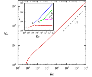
Figure 1. (a) The Nusselt number versus the Rayleigh number tracked from the energy stability bifurcation point. The solution to the background upper bounding problem is optimised over the domain length and the data are in excellent agreement with Hassanzadeh et al. (Reference Hassanzadeh, Chini and Doering2014) (their data courtesy of Dr A. Souza). Insets show the flow streamfunctions at $Ra=10^{5}$
and 106. (b) The optimal domain size
$Ra=10^{5}$
and 106. (b) The optimal domain size $L^{\ast }$
versus the Rayleigh number. The bullet is the energy stability bifurcation point.
$L^{\ast }$
versus the Rayleigh number. The bullet is the energy stability bifurcation point.

Figure 2. The first ( $\unicode[STIX]{x1D706}_{1}$
) and second (
$\unicode[STIX]{x1D706}_{1}$
) and second ( $\unicode[STIX]{x1D706}_{2}$
) largest eigenvalues of the spectral constraint for
$\unicode[STIX]{x1D706}_{2}$
) largest eigenvalues of the spectral constraint for $Ra<4468.8$
. At
$Ra<4468.8$
. At $Ra=4468.8$
, where they cross, the aspect ratio is
$Ra=4468.8$
, where they cross, the aspect ratio is $L^{\ast }=2.234$
.
$L^{\ast }=2.234$
.
3 Connecting to Hassanzadeh et al. (Reference Hassanzadeh, Chini and Doering2014)
The conductive temperature profile $\unicode[STIX]{x1D70F}=1-z$
is a spectrally stable background field until
$\unicode[STIX]{x1D70F}=1-z$
is a spectrally stable background field until $Ra=27\unicode[STIX]{x03C0}^{4}/4$
in a domain of size
$Ra=27\unicode[STIX]{x03C0}^{4}/4$
in a domain of size $L=2\sqrt{2}$
when energy instability first starts. Ensuring that the marginal fluctuation fields
$L=2\sqrt{2}$
when energy instability first starts. Ensuring that the marginal fluctuation fields $(\unicode[STIX]{x1D703},\unicode[STIX]{x1D713})$
– hereafter a mode – stay marginal (called pinning as was done in PK03), the optimal solution was then tracked up to
$(\unicode[STIX]{x1D703},\unicode[STIX]{x1D713})$
– hereafter a mode – stay marginal (called pinning as was done in PK03), the optimal solution was then tracked up to $Ra=10^{7}$
with the domain size
$Ra=10^{7}$
with the domain size $L=L^{\ast }(Ra)$
simultaneously optimised to yield the highest heat flux at a given
$L=L^{\ast }(Ra)$
simultaneously optimised to yield the highest heat flux at a given $Ra$
(see figure 1). The calculated
$Ra$
(see figure 1). The calculated $Nu$
values correspond exactly with those found by Hassanzadeh et al. (Reference Hassanzadeh, Chini and Doering2014) (as do flow fields computed at
$Nu$
values correspond exactly with those found by Hassanzadeh et al. (Reference Hassanzadeh, Chini and Doering2014) (as do flow fields computed at $Ra=10^{5}$
and 106; see the inset of figure 1). This indicates that Hassanzadeh et al.’s (Reference Hassanzadeh, Chini and Doering2014) wall-to-wall transport approach is equivalent to the background method when a single mode is considered.
$Ra=10^{5}$
and 106; see the inset of figure 1). This indicates that Hassanzadeh et al.’s (Reference Hassanzadeh, Chini and Doering2014) wall-to-wall transport approach is equivalent to the background method when a single mode is considered.

Figure 3. At $Ra=4468.8$
, the first mode (a)
$Ra=4468.8$
, the first mode (a) $\unicode[STIX]{x1D713}_{1}$
and (b)
$\unicode[STIX]{x1D713}_{1}$
and (b) $\unicode[STIX]{x1D703}_{1}$
and the new second mode (c)
$\unicode[STIX]{x1D703}_{1}$
and the new second mode (c) $\unicode[STIX]{x1D713}_{2}$
and (d)
$\unicode[STIX]{x1D713}_{2}$
and (d) $\unicode[STIX]{x1D703}_{2}$
.
$\unicode[STIX]{x1D703}_{2}$
.
In their wall-to-wall optimal control approach, however, Hassanzadeh et al. (Reference Hassanzadeh, Chini and Doering2014) had no way of identifying whether their local optimal was in fact the global optimal. It should be sufficiently close to the energy stability point but experience in other related problems (e.g. PK03) suggests that further modes in the spectral constraint eventually become marginal as $Ra$
increases. The optimal solution should subsequently modify itself to keep these new modes marginal with concomitant adjustments in the
$Ra$
increases. The optimal solution should subsequently modify itself to keep these new modes marginal with concomitant adjustments in the $Nu$
-scaling. Fortunately, in the background approach, the spectral constraint provides a check on whether a given Euler–Lagrange solution is the optimal solution. Solving the eigenvalue problem (2.13)–(2.14) for disturbances which are also periodic over
$Nu$
-scaling. Fortunately, in the background approach, the spectral constraint provides a check on whether a given Euler–Lagrange solution is the optimal solution. Solving the eigenvalue problem (2.13)–(2.14) for disturbances which are also periodic over $[0,L^{\ast }(Ra)]$
demonstrates that the eigenvalue (
$[0,L^{\ast }(Ra)]$
demonstrates that the eigenvalue ( $\unicode[STIX]{x1D706}_{1}$
in figure 2) of the first mode is pinned at 0, while a second mode becomes marginal at
$\unicode[STIX]{x1D706}_{1}$
in figure 2) of the first mode is pinned at 0, while a second mode becomes marginal at $Ra=4468.8$
for an aspect ratio
$Ra=4468.8$
for an aspect ratio $L^{\ast }=2.234$
. This suggests that Hassanzadeh et al.’s (Reference Hassanzadeh, Chini and Doering2014) result is either not a bound for
$L^{\ast }=2.234$
. This suggests that Hassanzadeh et al.’s (Reference Hassanzadeh, Chini and Doering2014) result is either not a bound for $Ra>4468.8$
or that the background bound has started to overestimate the actual maximal flux or, perhaps least likely, both. This divergence in results is apparently not because any further 2-D bifurcations have been missed in the wall-to-wall calculations (G. Chini, private communication 2019) but more a reflection of the ‘duality gap’ suggested by Souza et al. (Reference Souza, Tobasco and Doering2019) being realised. Figure 3(a,b) shows the first mode
$Ra>4468.8$
or that the background bound has started to overestimate the actual maximal flux or, perhaps least likely, both. This divergence in results is apparently not because any further 2-D bifurcations have been missed in the wall-to-wall calculations (G. Chini, private communication 2019) but more a reflection of the ‘duality gap’ suggested by Souza et al. (Reference Souza, Tobasco and Doering2019) being realised. Figure 3(a,b) shows the first mode $(\unicode[STIX]{x1D713}_{1},\unicode[STIX]{x1D703}_{1})$
with wavenumber
$(\unicode[STIX]{x1D713}_{1},\unicode[STIX]{x1D703}_{1})$
with wavenumber $\unicode[STIX]{x1D6FC}_{1}:=2\unicode[STIX]{x03C0}/L^{\ast }$
so the flow field contains one pair of convection cells. The second mode (
$\unicode[STIX]{x1D6FC}_{1}:=2\unicode[STIX]{x03C0}/L^{\ast }$
so the flow field contains one pair of convection cells. The second mode ( $\unicode[STIX]{x1D713}_{2},\unicode[STIX]{x1D703}_{2}$
) with
$\unicode[STIX]{x1D713}_{2},\unicode[STIX]{x1D703}_{2}$
) with $\unicode[STIX]{x1D6FC}_{2}=2\unicode[STIX]{x1D6FC}_{1}$
illustrated in figure 3(c,d) has two pairs of convection cells. The optimal background field at
$\unicode[STIX]{x1D6FC}_{2}=2\unicode[STIX]{x1D6FC}_{1}$
illustrated in figure 3(c,d) has two pairs of convection cells. The optimal background field at $Ra=2000$
is shown in figure 4(a) and the now non-optimal 1-mode solution at
$Ra=2000$
is shown in figure 4(a) and the now non-optimal 1-mode solution at $Ra=20\,000$
is shown in figure 4(b). In both cases the field is weakly two-dimensional, indicating that the first mode consists of non-monochromatic (i.e. non-single
$Ra=20\,000$
is shown in figure 4(b). In both cases the field is weakly two-dimensional, indicating that the first mode consists of non-monochromatic (i.e. non-single $\unicode[STIX]{x1D6FC}$
) velocity and temperature fields. The emergence of the second mode at
$\unicode[STIX]{x1D6FC}$
) velocity and temperature fields. The emergence of the second mode at $Ra=4468.8$
indicates that the background profile is now degenerate in a way which has important implications for solving the Euler–Lagrange equations for higher
$Ra=4468.8$
indicates that the background profile is now degenerate in a way which has important implications for solving the Euler–Lagrange equations for higher $Ra$
while respecting the spectral constraint. We discuss this issue in the following section.
$Ra$
while respecting the spectral constraint. We discuss this issue in the following section.

Figure 4. (a) The optimal background field $\unicode[STIX]{x1D70F}$
plotted at
$\unicode[STIX]{x1D70F}$
plotted at $Ra=2000$
and (b) the non-optimal 1-mode solution at
$Ra=2000$
and (b) the non-optimal 1-mode solution at $Ra=20\,000$
.
$Ra=20\,000$
.
4 Multi-modal optimals
When a new mode becomes marginal in the spectral constraint as the background field $\unicode[STIX]{x1D70F}$
evolves with
$\unicode[STIX]{x1D70F}$
evolves with $Ra$
, a further ‘pinning’ constraint needs to be added to keep the new mode marginal in the spectral constraint as
$Ra$
, a further ‘pinning’ constraint needs to be added to keep the new mode marginal in the spectral constraint as $Ra$
increases further. This procedure is thoroughly discussed in Doering & Constantin (Reference Doering and Constantin1996) and implemented in PK03 for a background field of lower dimensionality than the fluctuation field. In this situation, an example of which is using a 1-D case
$Ra$
increases further. This procedure is thoroughly discussed in Doering & Constantin (Reference Doering and Constantin1996) and implemented in PK03 for a background field of lower dimensionality than the fluctuation field. In this situation, an example of which is using a 1-D case $\unicode[STIX]{x1D70F}=\unicode[STIX]{x1D70F}(z)$
in the 2-D Rayleigh–Bénard problem, the fluctuation field can be Fourier transformed over the spatial dimension(s) across which
$\unicode[STIX]{x1D70F}=\unicode[STIX]{x1D70F}(z)$
in the 2-D Rayleigh–Bénard problem, the fluctuation field can be Fourier transformed over the spatial dimension(s) across which $\unicode[STIX]{x1D70F}$
is invariant and then considered parameterised by the Fourier wavenumber
$\unicode[STIX]{x1D70F}$
is invariant and then considered parameterised by the Fourier wavenumber $k$
. Different spectrally marginal fluctuation fields have different
$k$
. Different spectrally marginal fluctuation fields have different $k$
and are then naturally orthogonal under averaging over this spatial dimension. This means that the Euler–Lagrange equations (2.15)–(2.18),
$k$
and are then naturally orthogonal under averaging over this spatial dimension. This means that the Euler–Lagrange equations (2.15)–(2.18),
 $$\begin{eqnarray}\displaystyle & \displaystyle 0=\unicode[STIX]{x1D6FB}^{2}\unicode[STIX]{x1D703}_{j}-J(\unicode[STIX]{x1D70F},\unicode[STIX]{x1D713}_{j}),\quad j=1,\ldots ,N & \displaystyle\end{eqnarray}$$
 $$\begin{eqnarray}\displaystyle & \displaystyle 0=\frac{a}{Ra}\unicode[STIX]{x1D6FB}^{4}\unicode[STIX]{x1D713}_{i}-J(\unicode[STIX]{x1D70F},\unicode[STIX]{x1D703}_{i}),\quad j=1,\ldots ,N & \displaystyle\end{eqnarray}$$
 $$\begin{eqnarray}\displaystyle & \displaystyle 0=\unicode[STIX]{x1D70F}_{zz}-\mathop{\sum }_{j=1}^{N}\overline{J(\unicode[STIX]{x1D703}_{j},\unicode[STIX]{x1D713}_{j})}, & \displaystyle\end{eqnarray}$$
 $$\begin{eqnarray}\displaystyle & \displaystyle \langle |\unicode[STIX]{x1D70F}_{z}|^{2}\rangle -1={\displaystyle \frac{(1-a)}{Ra}}\mathop{\sum }_{j=1}^{N}\langle |\unicode[STIX]{x1D6FB}^{2}\unicode[STIX]{x1D713}_{j}|^{2}\rangle , & \displaystyle\end{eqnarray}$$
(the overbar represents averaging over $x$
) can simply be extended to include the new marginal mode
$x$
) can simply be extended to include the new marginal mode
 $$\begin{eqnarray}(\unicode[STIX]{x1D703}_{N+1},\unicode[STIX]{x1D713}_{N+1})(x,z)=(\hat{\unicode[STIX]{x1D703}}_{N+1},\hat{\unicode[STIX]{x1D713}}_{N+1})(z)\text{e}^{\text{i}k_{N+1}x}\end{eqnarray}$$
when it appears. Equivalently, the Lagrangian is just
 $$\begin{eqnarray}\mathscr{L}=\frac{1}{1-a}[\langle {\unicode[STIX]{x1D70F}_{z}}^{2}\rangle -a]-\frac{1}{1-a}\mathscr{G},\end{eqnarray}$$
where $\mathscr{G}$
naturally partitions into the contributions from the various marginal modes as follows:
$\mathscr{G}$
naturally partitions into the contributions from the various marginal modes as follows:
 $$\begin{eqnarray}\mathscr{G}=\left\langle \frac{a}{Ra}|\unicode[STIX]{x1D6FB}^{2}\unicode[STIX]{x1D713}|^{2}+|\unicode[STIX]{x1D735}\unicode[STIX]{x1D703}|^{2}+2\unicode[STIX]{x1D703}J(\unicode[STIX]{x1D70F},\unicode[STIX]{x1D713})\right\rangle =\mathop{\sum }_{j=1}^{N+1}\mathscr{G}_{j},\end{eqnarray}$$
where
 $$\begin{eqnarray}\mathscr{G}_{j}:=\left\langle \frac{a}{Ra}|\unicode[STIX]{x1D6FB}^{2}\unicode[STIX]{x1D713}_{j}|^{2}+|\unicode[STIX]{x1D735}\unicode[STIX]{x1D703}_{j}|^{2}+2\unicode[STIX]{x1D703}J(\unicode[STIX]{x1D70F},\unicode[STIX]{x1D713}_{j})\right\rangle .\end{eqnarray}$$
The appearance of a new spectrally marginal mode merely extends the set of wavenumbers contributing to the definition of the fluctuation field by one,
 $$\begin{eqnarray}(\unicode[STIX]{x1D713},\unicode[STIX]{x1D703})(x,z):=\mathop{\sum }_{j=1}^{N+1}(\unicode[STIX]{x1D713}_{j},\unicode[STIX]{x1D703}_{j})=\mathop{\sum }_{j=1}^{N+1}(\hat{\unicode[STIX]{x1D713}}_{j},\hat{\unicode[STIX]{x1D703}}_{j})(z)\text{e}^{\text{i}k_{j}x}.\end{eqnarray}$$
Importantly, this means it is possible to talk about the unique optimal solution of the variational problem which satisfies the imposed physical constraints as being
 $$\begin{eqnarray}(\unicode[STIX]{x1D713},T)(x,z)=(0,\unicode[STIX]{x1D70F})(z)+\mathop{\sum }_{j=1}^{N}(\hat{\unicode[STIX]{x1D713}}_{j},\hat{\unicode[STIX]{x1D703}}_{j})(z)\text{e}^{\text{i}k_{j}x},\end{eqnarray}$$
i.e. the spectral constraint is satisfied at a saddle point of $\mathscr{L}$
.
$\mathscr{L}$
.
This pleasing situation in which the marginal fluctuation fields have a physical interpretation changes, however, when the dimensionality of the background field equals the dimensionality of the problem (the case here), or, pathologically, there is more than one marginal mode for a given wavenumber (see chap. 3 of Fantuzzi Reference Fantuzzi2018). In these scenarios, the natural orthogonality property of different marginal fluctuation fields disappears with the result that the physical meaning of the fluctuation fields is lost. To see this, the key is to realise that pinning the marginal fluctuation fields is done (Doering & Constantin Reference Doering and Constantin1996) as before by writing the Lagrangian as
 $$\begin{eqnarray}\mathscr{L}=\frac{1}{1-a}(\langle |\unicode[STIX]{x1D735}\unicode[STIX]{x1D70F}|^{2}\rangle -a)-\frac{1}{1-a}\mathop{\sum }_{j=1}\mathscr{G}_{j}.\end{eqnarray}$$
The constraint that each $\mathscr{G}_{j}$
vanishes pins the
$\mathscr{G}_{j}$
vanishes pins the $j$
th mode to be marginal (the Lagrange multiplier imposing this is absorbed into the amplitude of the
$j$
th mode to be marginal (the Lagrange multiplier imposing this is absorbed into the amplitude of the $j$
th marginal fluctuation field) while
$j$
th marginal fluctuation field) while $\mathscr{G}>0$
for all other fluctuation fields. However, since the modes
$\mathscr{G}>0$
for all other fluctuation fields. However, since the modes $(\unicode[STIX]{x1D713}_{j},\unicode[STIX]{x1D703}_{j})$
are not now orthogonal,
$(\unicode[STIX]{x1D713}_{j},\unicode[STIX]{x1D703}_{j})$
are not now orthogonal,
 $$\begin{eqnarray}\mathop{\sum }_{j=1}^{N}\mathscr{G}_{j}\neq \mathscr{G}:=\left\langle \frac{b}{Ra}|\unicode[STIX]{x1D6FB}^{2}\unicode[STIX]{x1D713}|^{2}+|\unicode[STIX]{x1D735}\unicode[STIX]{x1D703}|^{2}+2\unicode[STIX]{x1D703}J(\unicode[STIX]{x1D70F},\unicode[STIX]{x1D713})\right\rangle ,\end{eqnarray}$$
for $N\geqslant 2$
where
$N\geqslant 2$
where
 $$\begin{eqnarray}(\unicode[STIX]{x1D713},\unicode[STIX]{x1D703})(x,z)=\mathop{\sum }_{j=1}^{N}(\unicode[STIX]{x1D713}_{j},\unicode[STIX]{x1D703}_{j})(x,z)\end{eqnarray}$$
is taken as the total optimal fluctuation field. In fact, $\mathscr{G}>0$
and so this total optimal field is not a solution of the heat equation. The clear implication is that the spectral constraint is not satisfied for
$\mathscr{G}>0$
and so this total optimal field is not a solution of the heat equation. The clear implication is that the spectral constraint is not satisfied for $N\geqslant 2$
at any saddle point of the Lagrangian (2.7) where the steady heat equation is imposed. Consequently, the optimisation procedure is forced to find an optimal away from the saddle points of the Lagrangian (2.7) where the spectral constraint is satisfied to deliver a bound.
$N\geqslant 2$
at any saddle point of the Lagrangian (2.7) where the steady heat equation is imposed. Consequently, the optimisation procedure is forced to find an optimal away from the saddle points of the Lagrangian (2.7) where the spectral constraint is satisfied to deliver a bound.
The fact that the form of the Lagrangian in (4.11) is different from that in (2.7) warrants further explanation. The Lagrangian in (2.7) is constructed in the usual way from the functional to be maximised (the heat flux) and the constraints to be applied with the highest stationary point being the maximal heat flux under the imposed constraints. The background method adds a further constraint by restricting the set of fields over which the Lagrangian is made stationary. Specifically, the allowed set (2.10) guarantees that any $(\unicode[STIX]{x1D70F},a)\in \unicode[STIX]{x1D6FA}$
will give a value of the Lagrangian greater or equal to that at the highest stationary point: see the discussion in § 2.2. When the background temperature field is of lower dimension than the physical problem – specifically here
$(\unicode[STIX]{x1D70F},a)\in \unicode[STIX]{x1D6FA}$
will give a value of the Lagrangian greater or equal to that at the highest stationary point: see the discussion in § 2.2. When the background temperature field is of lower dimension than the physical problem – specifically here $\unicode[STIX]{x1D70F}=\unicode[STIX]{x1D70F}(z)$
in 2-D Rayleigh–Bénard convection, this extra requirement emerges naturally from the Lagrangian (2.7) since
$\unicode[STIX]{x1D70F}=\unicode[STIX]{x1D70F}(z)$
in 2-D Rayleigh–Bénard convection, this extra requirement emerges naturally from the Lagrangian (2.7) since
 $$\begin{eqnarray}\mathscr{G}=\mathop{\sum }_{j=1}^{N}\mathscr{G}_{j}\end{eqnarray}$$
as the contributions to $\mathscr{G}$
from the various critical wavenumbers naturally separate. Put another way, the Lagrangians (4.11) and (2.7) are one and the same in this situation. There is, however, a further check that all other wavenumbers give
$\mathscr{G}$
from the various critical wavenumbers naturally separate. Put another way, the Lagrangians (4.11) and (2.7) are one and the same in this situation. There is, however, a further check that all other wavenumbers give $\mathscr{G}>0$
, which gets added onto the process of making the Lagrangian (2.7) stationary. Now, if
$\mathscr{G}>0$
, which gets added onto the process of making the Lagrangian (2.7) stationary. Now, if $\unicode[STIX]{x1D70F}$
has the same dimension as the physical problem, then the spectral problem also has the same dimension as the physical problem and (4.14) no longer holds (unless, trivially,
$\unicode[STIX]{x1D70F}$
has the same dimension as the physical problem, then the spectral problem also has the same dimension as the physical problem and (4.14) no longer holds (unless, trivially, $N=1$
). In this case the Lagrangian (2.7) has to be modified to that in (4.11) and the optimal solution no longer corresponds with the highest stationary point of (2.7). Instead, the highest stationary point of (4.11) will overestimate the highest stationary point of (2.7) as soon as
$N=1$
). In this case the Lagrangian (2.7) has to be modified to that in (4.11) and the optimal solution no longer corresponds with the highest stationary point of (2.7). Instead, the highest stationary point of (4.11) will overestimate the highest stationary point of (2.7) as soon as $N\geqslant 2$
and in particular, the constraints imposed directly in (2.7) will not be satisfied.
$N\geqslant 2$
and in particular, the constraints imposed directly in (2.7) will not be satisfied.
From a different perspective, Souza et al. (Reference Souza, Tobasco and Doering2019) have also recently argued that this should happen when exploring the connection between the wall-to-wall approach (a max–min problem) with the associated background method (a min–max problem). A duality gap means that
 $$\begin{eqnarray}(\text{wall-to-wall})\quad \sup _{\unicode[STIX]{x1D703},\boldsymbol{u}}\,\inf _{\unicode[STIX]{x1D70F}}\mathscr{L}<\inf _{\unicode[STIX]{x1D70F}}\sup _{\unicode[STIX]{x1D703},\boldsymbol{u}}\mathscr{L}\quad (\text{background}),\end{eqnarray}$$
(making the connection $\unicode[STIX]{x1D702}=\unicode[STIX]{x1D70F}-(1-z)$
and
$\unicode[STIX]{x1D702}=\unicode[STIX]{x1D70F}-(1-z)$
and $\unicode[STIX]{x1D701}=\unicode[STIX]{x1D703}$
with the variables used by Souza et al. (Reference Souza, Tobasco and Doering2019)) where the optimal solution to the wall-to-wall problem is achieved at a stationary point of
$\unicode[STIX]{x1D701}=\unicode[STIX]{x1D703}$
with the variables used by Souza et al. (Reference Souza, Tobasco and Doering2019)) where the optimal solution to the wall-to-wall problem is achieved at a stationary point of $\mathscr{L}$
, thereby implying that to the background method is not. They also supply a simple quadratic polynomial in five variables to illustrate the phenomenon. The calculations described in the next section confirm that this gap starts to exist as soon as
$\mathscr{L}$
, thereby implying that to the background method is not. They also supply a simple quadratic polynomial in five variables to illustrate the phenomenon. The calculations described in the next section confirm that this gap starts to exist as soon as $N=2$
.
$N=2$
.

Figure 5. (a) The Nusselt number $Nu$
versus the Rayleigh number
$Nu$
versus the Rayleigh number $Ra$
at fixed aspect ratio
$Ra$
at fixed aspect ratio $L=2\sqrt{2}$
. (b)
$L=2\sqrt{2}$
. (b) $Nu$
versus
$Nu$
versus $\unicode[STIX]{x1D6FC}=2\unicode[STIX]{x03C0}/L$
.
$\unicode[STIX]{x1D6FC}=2\unicode[STIX]{x03C0}/L$
.
5 Extending Hassanzedah et al. with a symmetric 2-D background field
$\unicode[STIX]{x1D70F}(x,z)$

To explore multi-modal bounding solutions, a first series of computations was done in the fixed domain $L=2\sqrt{2}$
. In this geometry, the first mode appears at
$L=2\sqrt{2}$
. In this geometry, the first mode appears at $Ra=27\unicode[STIX]{x03C0}^{4}/4$
(the energy stability threshold), the second mode at
$Ra=27\unicode[STIX]{x03C0}^{4}/4$
(the energy stability threshold), the second mode at $Ra=3,075$
and the third mode at
$Ra=3,075$
and the third mode at $Ra=24\,650$
. The 1-mode and 2-mode optimal solution branches could be easily continued up to
$Ra=24\,650$
. The 1-mode and 2-mode optimal solution branches could be easily continued up to $Ra=10^{5}$
whereas the 3-mode solution branch proved difficult to continue much beyond
$Ra=10^{5}$
whereas the 3-mode solution branch proved difficult to continue much beyond $Ra>40\,000$
due to numerical issues: see figure 5(a). The 3-mode solution, which provides an upper bound in this geometry over at least the range
$Ra>40\,000$
due to numerical issues: see figure 5(a). The 3-mode solution, which provides an upper bound in this geometry over at least the range $24\,650\leqslant Ra\leqslant 40\,000$
, presents only a modest correction to the 2-mode optimal solution which is no longer a bound for these
$24\,650\leqslant Ra\leqslant 40\,000$
, presents only a modest correction to the 2-mode optimal solution which is no longer a bound for these $Ra$
.
$Ra$
.
A second series of computations were then carried out to investigate the dependence of the $Nu$
-bound on the aspect ratio
$Nu$
-bound on the aspect ratio $L$
. Three different
$L$
. Three different $Ra$
values were chosen to explore the dependence of the bound on
$Ra$
values were chosen to explore the dependence of the bound on $L$
:
$L$
: $Ra=5000$
and 10 000 where the bound is given by a 2-mode solution, and
$Ra=5000$
and 10 000 where the bound is given by a 2-mode solution, and $Ra=25\,000$
where the bound is given by a 3-mode solution. In all three cases, the largest bound is achieved as the aspect ratio
$Ra=25\,000$
where the bound is given by a 3-mode solution. In all three cases, the largest bound is achieved as the aspect ratio $L\rightarrow \infty$
; see figure 5(b). This is very different from the optimal control results of Hassanzadeh et al. (Reference Hassanzadeh, Chini and Doering2014), where the optimal aspect ratio scales like
$L\rightarrow \infty$
; see figure 5(b). This is very different from the optimal control results of Hassanzadeh et al. (Reference Hassanzadeh, Chini and Doering2014), where the optimal aspect ratio scales like $Ra^{-1/4}$
and so vanishes as
$Ra^{-1/4}$
and so vanishes as $Ra\rightarrow \infty$
.
$Ra\rightarrow \infty$
.
Figure 6 shows the structure of the two modes at $Ra=10^{4}$
. The fluctuation fields
$Ra=10^{4}$
. The fluctuation fields $\unicode[STIX]{x1D713}_{i}$
and
$\unicode[STIX]{x1D713}_{i}$
and $\unicode[STIX]{x1D703}_{i}$
for both
$\unicode[STIX]{x1D703}_{i}$
for both $i=1$
and 2 have a convection roll structure and increasing
$i=1$
and 2 have a convection roll structure and increasing $L$
just means that more of the rolls fit into the domain. On closer inspection it is clear that the rolls are slightly different near to
$L$
just means that more of the rolls fit into the domain. On closer inspection it is clear that the rolls are slightly different near to $x=0$
and
$x=0$
and $x=\pm \frac{1}{2}L$
where they are forced to have a certain symmetry (symmetry around
$x=\pm \frac{1}{2}L$
where they are forced to have a certain symmetry (symmetry around $x=0$
and periodicity over a length
$x=0$
and periodicity over a length $L$
force symmetry about
$L$
force symmetry about $x=\pm \frac{1}{2}L$
as well). When the domain is short, e.g.
$x=\pm \frac{1}{2}L$
as well). When the domain is short, e.g. $L=\unicode[STIX]{x03C0}$
, the background field is clearly two-dimensional as seen in figure 7. However, as
$L=\unicode[STIX]{x03C0}$
, the background field is clearly two-dimensional as seen in figure 7. However, as $L$
increases to
$L$
increases to $L=8\unicode[STIX]{x03C0}$
, the background field become predominantly one-dimensional away from the imposed lines of symmetry at
$L=8\unicode[STIX]{x03C0}$
, the background field become predominantly one-dimensional away from the imposed lines of symmetry at $x=0$
and
$x=0$
and $x=\pm \frac{1}{2}L$
(the ends of the domain shown). Plotting the streamfunctions
$x=\pm \frac{1}{2}L$
(the ends of the domain shown). Plotting the streamfunctions $\unicode[STIX]{x1D713}_{1}$
and
$\unicode[STIX]{x1D713}_{1}$
and $\unicode[STIX]{x1D713}_{2}$
over this long domain – see figure 8 – confirms that the convection cells are similar away from the symmetry lines (‘zone 1’ in figure 8) where
$\unicode[STIX]{x1D713}_{2}$
over this long domain – see figure 8 – confirms that the convection cells are similar away from the symmetry lines (‘zone 1’ in figure 8) where $\unicode[STIX]{x1D70F}$
is predominantly one-dimensional but are quite different close to the symmetry lines (‘zone 2’) where
$\unicode[STIX]{x1D70F}$
is predominantly one-dimensional but are quite different close to the symmetry lines (‘zone 2’) where $\unicode[STIX]{x1D70F}$
is clearly two-dimensional.
$\unicode[STIX]{x1D70F}$
is clearly two-dimensional.
The structure of the optimal fields (both background and fluctuation) and the fact that the bound is maximised as $L\rightarrow \infty$
indicate that the optimal solution is trying to minimise the effect of the imposed symmetry requirements at
$L\rightarrow \infty$
indicate that the optimal solution is trying to minimise the effect of the imposed symmetry requirements at $x=0$
and
$x=0$
and $x=\pm \frac{1}{2}L$
. Without this imposed symmetry, the problem becomes translationally invariant and the optimal solution must be one-dimensional by the convexity result in § 2.3 (Doering & Constantin Reference Doering and Constantin1996). There is another simple way to see this. Since the bounding functional
$x=\pm \frac{1}{2}L$
. Without this imposed symmetry, the problem becomes translationally invariant and the optimal solution must be one-dimensional by the convexity result in § 2.3 (Doering & Constantin Reference Doering and Constantin1996). There is another simple way to see this. Since the bounding functional $f(\unicode[STIX]{x1D70F},a)$
(see (2.19)) is strictly convex in both
$f(\unicode[STIX]{x1D70F},a)$
(see (2.19)) is strictly convex in both $\unicode[STIX]{x1D70F}(x,z)$
and
$\unicode[STIX]{x1D70F}(x,z)$
and $a$
, any 2-D solution
$a$
, any 2-D solution $(\unicode[STIX]{x1D70F}_{2D}(x,z),a)\in \unicode[STIX]{x1D6FA}$
satisfies
$(\unicode[STIX]{x1D70F}_{2D}(x,z),a)\in \unicode[STIX]{x1D6FA}$
satisfies
 $$\begin{eqnarray}f\left(\frac{1}{N}\mathop{\sum }_{j=1}^{N}\unicode[STIX]{x1D70F}_{2D}\left(x+\frac{jL}{N},z\right),a\right)<\frac{1}{N}\mathop{\sum }_{j=1}^{N}f\left(\unicode[STIX]{x1D70F}_{2D}\left(x+\frac{jL}{N},z\right),a\right)\end{eqnarray}$$
by Jensen’s inequality. Taking the limit $N\rightarrow \infty$
on the left-hand side and using translational invariance of the problem on the right-hand side leads to
$N\rightarrow \infty$
on the left-hand side and using translational invariance of the problem on the right-hand side leads to
 $$\begin{eqnarray}f\left(\unicode[STIX]{x1D70F}_{1\text{D}}(z):=\frac{1}{L}\int _{0}^{L}\unicode[STIX]{x1D70F}_{2D}(x,z)\,\text{d}x,a\right)<f(\unicode[STIX]{x1D70F}_{2D}(x,z),a),\end{eqnarray}$$
so that a 1-D background field always produces a better bound than a 2-D field. The results in figure 7 indicate that this is what the optimal solution to the background problem is trying to achieve.

Figure 6. (a) The first mode ( $\unicode[STIX]{x1D713}_{1},\unicode[STIX]{x1D703}_{1}$
); (b) the second mode (
$\unicode[STIX]{x1D713}_{1},\unicode[STIX]{x1D703}_{1}$
); (b) the second mode ( $\unicode[STIX]{x1D713}_{2},\unicode[STIX]{x1D703}_{2}$
) at
$\unicode[STIX]{x1D713}_{2},\unicode[STIX]{x1D703}_{2}$
) at $Ra=10^{4}$
(only two critical modes are present for this
$Ra=10^{4}$
(only two critical modes are present for this $Ra$
).
$Ra$
).

Figure 7. The background field plotted at different aspect ratios at $Ra=10^{4}$
.
$Ra=10^{4}$
.

Figure 8. The two critical flow fields at $Ra=10^{4}$
and
$Ra=10^{4}$
and $L=8\unicode[STIX]{x03C0}$
: (a)
$L=8\unicode[STIX]{x03C0}$
: (a) $\unicode[STIX]{x1D713}_{1}$
and (b)
$\unicode[STIX]{x1D713}_{1}$
and (b) $\unicode[STIX]{x1D713}_{2}$
.
$\unicode[STIX]{x1D713}_{2}$
.
5.1 Lifting the symmetry: 1-D background field
Calculation of the optimal solution assuming from the onset that the background field is one-dimensional simplifies the computation since the fluctuation fields can then be parametrised by their single wavenumber in $x$
(as in (4.5)). In this case, rather than setting a domain periodicity and insisting the fluctuation wavenumbers be consistent with this, the wavenumbers themselves can be optimised over as real continuous variables meaning, in effect, that
$x$
(as in (4.5)). In this case, rather than setting a domain periodicity and insisting the fluctuation wavenumbers be consistent with this, the wavenumbers themselves can be optimised over as real continuous variables meaning, in effect, that $L$
is infinite. For example, the Euler–Lagrange equation corresponding to the
$L$
is infinite. For example, the Euler–Lagrange equation corresponding to the $m$
th wavenumber
$m$
th wavenumber $k_{m}$
is
$k_{m}$
is
 $$\begin{eqnarray}\unicode[STIX]{x1D6FF}\mathscr{L}/\unicode[STIX]{x1D6FF}k_{m}:=-2\int _{0}^{1}ak_{m}(u_{m}^{2}+w_{m}^{2})+k_{m}\unicode[STIX]{x1D703}_{m}^{2}\,\text{d}z+\int _{0}^{1}p_{m}u_{m}\,\text{d}z=0.\end{eqnarray}$$
With this formulation, Newton’s method with branch continuation proved much faster than the time stepping approach. It took approximately 4 h CPU time on a 2.8 GHz laptop using Newton’s method to obtain the optimal solution from $Ra=27\unicode[STIX]{x03C0}^{4}/4$
up to
$Ra=27\unicode[STIX]{x03C0}^{4}/4$
up to $Ra=5\times 10^{8}$
while the time stepping approach took at least a day to generate a single point at
$Ra=5\times 10^{8}$
while the time stepping approach took at least a day to generate a single point at $Ra=5\times 10^{8}$
. However, when the domain is fixed, Newton’s method becomes very inefficient as the critical wavenumbers
$Ra=5\times 10^{8}$
. However, when the domain is fixed, Newton’s method becomes very inefficient as the critical wavenumbers $k_{m}$
are discrete and cannot be tracked using a (continuous) continuation method: in this case, time stepping is the better choice. The numerical solution of the one-dimensional background problem gives the upper bound of
$k_{m}$
are discrete and cannot be tracked using a (continuous) continuation method: in this case, time stepping is the better choice. The numerical solution of the one-dimensional background problem gives the upper bound of $Nu\leqslant 0.055Ra^{1/2}$
, as shown in figure 9(a) with five critical modes present by
$Nu\leqslant 0.055Ra^{1/2}$
, as shown in figure 9(a) with five critical modes present by $Ra=10^{9}$
(see figure 9(b)). This result has the same scaling exponent as the non-slip result
$Ra=10^{9}$
(see figure 9(b)). This result has the same scaling exponent as the non-slip result $Nu\leqslant 0.026Ra^{1/2}$
of PK03 but with a larger numerical coefficient as should be expected for stress-free boundary conditions. The prior work of Wen et al. (Reference Wen, Chini, Kerswell and Doering2015) indicates that adding a further enstrophy constraint (possible only in stress-free 2-D convection) significantly improves the bound obtained here down to
$Nu\leqslant 0.026Ra^{1/2}$
of PK03 but with a larger numerical coefficient as should be expected for stress-free boundary conditions. The prior work of Wen et al. (Reference Wen, Chini, Kerswell and Doering2015) indicates that adding a further enstrophy constraint (possible only in stress-free 2-D convection) significantly improves the bound obtained here down to $Nu\leqslant 0.106Ra^{5/12}$
.
$Nu\leqslant 0.106Ra^{5/12}$
.

Figure 9. (a) The upper bound of $Nu$
versus the Rayleigh number
$Nu$
versus the Rayleigh number $Ra$
with
$Ra$
with $Nu\leqslant 0.055Ra^{1/2}$
in the asymptotic regime. (b) The bifurcation diagram of critical wavenumber
$Nu\leqslant 0.055Ra^{1/2}$
in the asymptotic regime. (b) The bifurcation diagram of critical wavenumber $k_{m}$
versus the Rayleigh number.
$k_{m}$
versus the Rayleigh number.
It is worth briefly discussing how the critical wavenumbers which appear in the 1-D and 2-D background field calculations are related. Figure 9(b) indicates that at $Ra=10^{4}$
there is only one critical wavenumber
$Ra=10^{4}$
there is only one critical wavenumber $k_{1}=3.284$
for the 1-D background problem. However, for the 2-D (symmetric) background problem, there are two critical modes, as seen in figure 6 and figure 8, with both having an approximate wavenumber ≈3. 3. Both these modes are forced to be antisymmetric (and so in phase) about
$k_{1}=3.284$
for the 1-D background problem. However, for the 2-D (symmetric) background problem, there are two critical modes, as seen in figure 6 and figure 8, with both having an approximate wavenumber ≈3. 3. Both these modes are forced to be antisymmetric (and so in phase) about $x=0$
and
$x=0$
and $x=\pm L/2$
(zone 2 in figure 8) but away from these points endeavour to be approximately
$x=\pm L/2$
(zone 2 in figure 8) but away from these points endeavour to be approximately $\unicode[STIX]{x03C0}/2$
out of phase (zone 1 in figure 8). With this phase difference together with matching amplitudes so
$\unicode[STIX]{x03C0}/2$
out of phase (zone 1 in figure 8). With this phase difference together with matching amplitudes so
 $$\begin{eqnarray}\displaystyle \unicode[STIX]{x1D713}_{1}=f(z)\sin (k_{1}x),\quad \unicode[STIX]{x1D703}_{1}=g(z)\cos (k_{1}x), & & \displaystyle\end{eqnarray}$$
 $$\begin{eqnarray}\displaystyle \unicode[STIX]{x1D713}_{2}=f(z)\sin (k_{1}x+\unicode[STIX]{x03C0}/2),\quad \unicode[STIX]{x1D703}_{2}=g(z)\cos (k_{1}x+\unicode[STIX]{x03C0}/2), & & \displaystyle\end{eqnarray}$$
the nonlinear term in (2.17)
 $$\begin{eqnarray}\mathop{\sum }_{i=1}^{2}\left[\frac{\unicode[STIX]{x2202}\unicode[STIX]{x1D713}_{i}}{\unicode[STIX]{x2202}z}\frac{\unicode[STIX]{x2202}\unicode[STIX]{x1D703}_{i}}{\unicode[STIX]{x2202}x}-\frac{\unicode[STIX]{x2202}\unicode[STIX]{x1D713}_{i}}{\unicode[STIX]{x2202}x}\frac{\unicode[STIX]{x2202}\unicode[STIX]{x1D703}_{i}}{\unicode[STIX]{x2202}z}\right]=-k_{1}\left[\frac{\text{d}f}{\text{d}z}g+\frac{\text{d}g}{\text{d}z}f\right]\end{eqnarray}$$
is $x$
independent and therefore can only drive a 1-D background field. From another perspective, the 1-D background field problem really has two modes with
$x$
independent and therefore can only drive a 1-D background field. From another perspective, the 1-D background field problem really has two modes with $k=3.284$
but only one needs to be tracked as the nonlinear term is horizontally averaged (e.g. see (4.3)) ensuring that the background field stays one-dimensional.
$k=3.284$
but only one needs to be tracked as the nonlinear term is horizontally averaged (e.g. see (4.3)) ensuring that the background field stays one-dimensional.
At $Ra=25\,000$
there is even a third mode in the 2-D background problem compared to still only 1 mode in the 1-D background problem (the second wavenumber
$Ra=25\,000$
there is even a third mode in the 2-D background problem compared to still only 1 mode in the 1-D background problem (the second wavenumber $k_{2}$
appears at
$k_{2}$
appears at $Ra\approx 26\,450$
). Figure 10 shows that in fact
$Ra\approx 26\,450$
). Figure 10 shows that in fact $\unicode[STIX]{x1D713}_{3}$
is only significant in zone 2 where the imposed symmetries dominate. In zone 1, where the background field is essentially a 1-D profile,
$\unicode[STIX]{x1D713}_{3}$
is only significant in zone 2 where the imposed symmetries dominate. In zone 1, where the background field is essentially a 1-D profile, $\unicode[STIX]{x1D713}_{3}$
vanishes.
$\unicode[STIX]{x1D713}_{3}$
vanishes.

Figure 10. (a–c) The profiles of the three critical flow fields $\unicode[STIX]{x1D713}_{1}$
,
$\unicode[STIX]{x1D713}_{1}$
, $\unicode[STIX]{x1D713}_{2}$
,
$\unicode[STIX]{x1D713}_{2}$
, $\unicode[STIX]{x1D713}_{3}$
at
$\unicode[STIX]{x1D713}_{3}$
at $Ra=25\,000$
,
$Ra=25\,000$
, $L=4\unicode[STIX]{x03C0}$
. (d) The profile of the two-dimensional optimal background field.
$L=4\unicode[STIX]{x03C0}$
. (d) The profile of the two-dimensional optimal background field.
The conclusion of the computations so far is that using a 2-D background temperature field does not improve the upper bound produced by a 1-D background temperature field, a realisation also reached independently in Doering & Tobasco (Reference Doering and Tobasco2019) (see their lemma 6.1). The next obvious question is whether adding a background velocity field helps either and we now turn our attention to this.
6 Imposing the steady momentum equation:
$\unicode[STIX]{x1D753}\neq \mathbf{0}$

In this section, we attempt to improve the bound by using a background temperature field and a background velocity field of the same dimension as the physical problem, which means that the full, albeit steady, momentum and heat equations are imposed as constraints. Importantly, the optimisation problem is no longer convex and so permitting $\unicode[STIX]{x1D753}\neq \mathbf{0}$
could produce a better (reduced) upper bound. However, numerical calculations suggest otherwise with
$\unicode[STIX]{x1D753}\neq \mathbf{0}$
could produce a better (reduced) upper bound. However, numerical calculations suggest otherwise with $\unicode[STIX]{x1D753}$
remaining zero after every bifurcation. To attempt to explain this, we use an inductive bifurcation analysis to show that if
$\unicode[STIX]{x1D753}$
remaining zero after every bifurcation. To attempt to explain this, we use an inductive bifurcation analysis to show that if $\unicode[STIX]{x1D753}=\mathbf{0}$
before a bifurcation then it remains
$\unicode[STIX]{x1D753}=\mathbf{0}$
before a bifurcation then it remains $\mathbf{0}$
after it too, implying that the continuous branch of optimals found by branch tracking out of the energy stability point always has
$\mathbf{0}$
after it too, implying that the continuous branch of optimals found by branch tracking out of the energy stability point always has $\unicode[STIX]{x1D753}=\mathbf{0}$
.
$\unicode[STIX]{x1D753}=\mathbf{0}$
.
The analysis begins by constructing the following Lagrangian:
 $$\begin{eqnarray}\mathscr{L}=\langle |\unicode[STIX]{x1D735}T|^{2}\rangle -\frac{a}{\unicode[STIX]{x1D70E}Ra}\langle \boldsymbol{v}\boldsymbol{\cdot }\boldsymbol{{\mathcal{N}}}\rangle -2\langle \unicode[STIX]{x1D703}{\mathcal{H}}\rangle ,\end{eqnarray}$$
which, after introducing the extended background decomposition
 $$\begin{eqnarray}\boldsymbol{u}=\unicode[STIX]{x1D753}+\boldsymbol{v},\quad T=\unicode[STIX]{x1D70F}+\unicode[STIX]{x1D703}\end{eqnarray}$$
(now both $\unicode[STIX]{x1D753}$
and
$\unicode[STIX]{x1D753}$
and $\boldsymbol{v}$
vanish on the boundaries
$\boldsymbol{v}$
vanish on the boundaries $z=0,1$
), can be rewritten as
$z=0,1$
), can be rewritten as
 $$\begin{eqnarray}\mathscr{L}=\frac{\langle |\unicode[STIX]{x1D735}\unicode[STIX]{x1D70F}|^{2}\rangle -a}{1-a}-\frac{a}{1-a}\langle \unicode[STIX]{x1D719}_{z}\unicode[STIX]{x1D70F}\rangle -\frac{1}{1-a}\mathscr{G},\end{eqnarray}$$
( $\unicode[STIX]{x1D719}_{z}:=\unicode[STIX]{x1D753}\boldsymbol{\cdot }\hat{\boldsymbol{z}}$
), where
$\unicode[STIX]{x1D719}_{z}:=\unicode[STIX]{x1D753}\boldsymbol{\cdot }\hat{\boldsymbol{z}}$
), where
 $$\begin{eqnarray}\displaystyle \mathscr{G}(\boldsymbol{v},\unicode[STIX]{x1D703}) & := & \displaystyle \langle 2\unicode[STIX]{x1D703}(\unicode[STIX]{x1D753}+\boldsymbol{v})\boldsymbol{\cdot }\unicode[STIX]{x1D735}\unicode[STIX]{x1D70F}+|\unicode[STIX]{x1D735}\unicode[STIX]{x1D703}|^{2}\rangle +a\langle \unicode[STIX]{x1D719}_{z}\unicode[STIX]{x1D703}\rangle \nonumber\\ \displaystyle & & \displaystyle +\,\left\langle \frac{a}{\unicode[STIX]{x1D70E}Ra}\boldsymbol{v}\boldsymbol{\cdot }\boldsymbol{v}\boldsymbol{\cdot }\unicode[STIX]{x1D735}\unicode[STIX]{x1D753}+\frac{a}{\unicode[STIX]{x1D70E}Ra}\boldsymbol{v}\boldsymbol{\cdot }\unicode[STIX]{x1D753}\boldsymbol{\cdot }\unicode[STIX]{x1D735}\unicode[STIX]{x1D753}+\frac{a}{Ra}|\unicode[STIX]{x1D735}\boldsymbol{v}|^{2}-\frac{a}{Ra}\boldsymbol{v}\boldsymbol{\cdot }\unicode[STIX]{x1D6FB}^{2}\unicode[STIX]{x1D753}\right\rangle \nonumber\end{eqnarray}$$
(note $\mathscr{G}$
depends parametrically on
$\mathscr{G}$
depends parametrically on $\unicode[STIX]{x1D70F}$
,
$\unicode[STIX]{x1D70F}$
, $\unicode[STIX]{x1D753}$
,
$\unicode[STIX]{x1D753}$
, $a$
,
$a$
, $\unicode[STIX]{x1D70E}$
and
$\unicode[STIX]{x1D70E}$
and $Ra$
but this is suppressed for clarity). If
$Ra$
but this is suppressed for clarity). If $\inf _{\boldsymbol{v},\unicode[STIX]{x1D703}}\mathscr{G}$
exists (and necessarily
$\inf _{\boldsymbol{v},\unicode[STIX]{x1D703}}\mathscr{G}$
exists (and necessarily $0<a<1$
), a bound is then given by
$0<a<1$
), a bound is then given by
 $$\begin{eqnarray}Nu\leqslant \frac{\langle |\unicode[STIX]{x1D735}\unicode[STIX]{x1D70F}|^{2}\rangle -a}{1-a}-\frac{a}{1-a}\langle \unicode[STIX]{x1D719}_{z}\unicode[STIX]{x1D70F}\rangle -\frac{1}{1-a}\inf _{\boldsymbol{v},\unicode[STIX]{x1D703}}\mathscr{G}(\unicode[STIX]{x1D70F},\unicode[STIX]{x1D753}).\end{eqnarray}$$
Minimisation of $\mathscr{G}$
with respect to incompressible
$\mathscr{G}$
with respect to incompressible $\boldsymbol{v}$
and
$\boldsymbol{v}$
and $\unicode[STIX]{x1D703}$
requires
$\unicode[STIX]{x1D703}$
requires
 $$\begin{eqnarray}\displaystyle & \displaystyle -{\displaystyle \frac{2a}{Ra}}\unicode[STIX]{x1D6FB}^{2}\boldsymbol{v}+\frac{a}{\unicode[STIX]{x1D70E}Ra}\boldsymbol{v}\boldsymbol{\cdot }(\unicode[STIX]{x1D735}\unicode[STIX]{x1D753}+\unicode[STIX]{x1D735}\unicode[STIX]{x1D753}^{\text{T}})+\frac{a}{\unicode[STIX]{x1D70E}Ra}\unicode[STIX]{x1D753}\boldsymbol{\cdot }\unicode[STIX]{x1D735}\unicode[STIX]{x1D753}-\frac{a}{\unicode[STIX]{x1D70E}Ra}\unicode[STIX]{x1D6FB}^{2}\unicode[STIX]{x1D753}+2\unicode[STIX]{x1D703}\unicode[STIX]{x1D735}\unicode[STIX]{x1D70F}+\unicode[STIX]{x1D735}p=0,\quad & \displaystyle\end{eqnarray}$$
 $$\begin{eqnarray}\displaystyle & \displaystyle \unicode[STIX]{x1D735}\boldsymbol{\cdot }\boldsymbol{v}=0, & \displaystyle\end{eqnarray}$$
 $$\begin{eqnarray}\displaystyle & \displaystyle -2\unicode[STIX]{x1D6FB}^{2}\unicode[STIX]{x1D703}+a\unicode[STIX]{x1D719}_{z}+2(\boldsymbol{v}+\unicode[STIX]{x1D753})\boldsymbol{\cdot }\unicode[STIX]{x1D735}\unicode[STIX]{x1D70F}=0, & \displaystyle\end{eqnarray}$$
the solution of which is denoted as $(\boldsymbol{v}_{0},\unicode[STIX]{x1D703}_{0})$
. The Lagrangian can then be written as
$(\boldsymbol{v}_{0},\unicode[STIX]{x1D703}_{0})$
. The Lagrangian can then be written as
 $$\begin{eqnarray}\mathscr{L}=\frac{\langle |\unicode[STIX]{x1D735}\unicode[STIX]{x1D70F}|^{2}\rangle -a}{1-a}-\frac{a}{1-a}\langle \unicode[STIX]{x1D719}_{z}\unicode[STIX]{x1D70F}\rangle -\frac{1}{1-a}\left\{\mathscr{G}(\boldsymbol{v}_{0},\unicode[STIX]{x1D703}_{0};\unicode[STIX]{x1D70F},\unicode[STIX]{x1D753})+\mathop{\sum }_{i=1}^{N}\mathscr{H}(\boldsymbol{v}_{i},\unicode[STIX]{x1D703}_{i})\right\},\end{eqnarray}$$
where $\boldsymbol{v}_{0}$
,
$\boldsymbol{v}_{0}$
, $\boldsymbol{v}_{i}$
(
$\boldsymbol{v}_{i}$
( $i=1\ldots N$
) and
$i=1\ldots N$
) and $\unicode[STIX]{x1D753}$
are incompressible fields and
$\unicode[STIX]{x1D753}$
are incompressible fields and
 $$\begin{eqnarray}\mathscr{H}(\boldsymbol{v},\unicode[STIX]{x1D703}):=\left\langle 2\unicode[STIX]{x1D703}\boldsymbol{v}\boldsymbol{\cdot }\unicode[STIX]{x1D735}\unicode[STIX]{x1D70F}+|\unicode[STIX]{x1D735}\unicode[STIX]{x1D703}|^{2}+\frac{a}{\unicode[STIX]{x1D70E}Ra}\boldsymbol{v}\boldsymbol{\cdot }\boldsymbol{v}\boldsymbol{\cdot }\unicode[STIX]{x1D735}\unicode[STIX]{x1D753}+\frac{a}{Ra}|\unicode[STIX]{x1D735}\boldsymbol{v}|^{2}\right\rangle\end{eqnarray}$$
is a purely quadratic functional of $(\boldsymbol{v},\unicode[STIX]{x1D703})$
which must be positive semi-definite – the spectral constraint – for
$(\boldsymbol{v},\unicode[STIX]{x1D703})$
which must be positive semi-definite – the spectral constraint – for $\inf \mathscr{G}$
to exist. The fields
$\inf \mathscr{G}$
to exist. The fields $(\boldsymbol{v}_{i},\unicode[STIX]{x1D703}_{i})$
are marginal in that
$(\boldsymbol{v}_{i},\unicode[STIX]{x1D703}_{i})$
are marginal in that $\mathscr{H}(\boldsymbol{v}_{i},\unicode[STIX]{x1D703}_{i})=0$
and their number
$\mathscr{H}(\boldsymbol{v}_{i},\unicode[STIX]{x1D703}_{i})=0$
and their number $N$
increases with
$N$
increases with $Ra$
. The aim is to minimise the upper bound over
$Ra$
. The aim is to minimise the upper bound over $\unicode[STIX]{x1D70F}$
,
$\unicode[STIX]{x1D70F}$
, $\unicode[STIX]{x1D753}$
and
$\unicode[STIX]{x1D753}$
and $a$
at fixed
$a$
at fixed $\unicode[STIX]{x1D70E}$
and
$\unicode[STIX]{x1D70E}$
and $Ra$
subject to this spectral constraint. The Euler–Lagrange equations are as follows: the spectral constraint equations for
$Ra$
subject to this spectral constraint. The Euler–Lagrange equations are as follows: the spectral constraint equations for $\boldsymbol{v}_{i}$
and
$\boldsymbol{v}_{i}$
and $\unicode[STIX]{x1D703}_{i}$
 $$\begin{eqnarray}\displaystyle \displaystyle -(1-a)Ra\frac{\unicode[STIX]{x1D6FF}\mathscr{L}}{\unicode[STIX]{x1D6FF}\boldsymbol{v}_{i}} & := & \displaystyle -2a\unicode[STIX]{x1D6FB}^{2}\boldsymbol{v}_{i}+\frac{a}{\unicode[STIX]{x1D70E}}\boldsymbol{v}_{i}\boldsymbol{\cdot }(\unicode[STIX]{x1D735}\unicode[STIX]{x1D753}+\unicode[STIX]{x1D735}\unicode[STIX]{x1D753}^{\text{T}})\nonumber\\ \displaystyle & & \displaystyle +\,2Ra\unicode[STIX]{x1D703}_{i}\unicode[STIX]{x1D735}\unicode[STIX]{x1D70F}+\unicode[STIX]{x1D735}p_{i}=\mathbf{0},\quad i=1\ldots N,\end{eqnarray}$$
 $$\begin{eqnarray}\displaystyle \displaystyle -(1-a)\frac{\unicode[STIX]{x1D6FF}\mathscr{L}}{\unicode[STIX]{x1D6FF}\unicode[STIX]{x1D703}_{i}}:=-2\unicode[STIX]{x1D6FB}^{2}\unicode[STIX]{x1D703}_{i}+2\boldsymbol{v}_{i}\boldsymbol{\cdot }\unicode[STIX]{x1D735}\unicode[STIX]{x1D70F}=0,\quad i=1\ldots N; & & \displaystyle\end{eqnarray}$$
the forced field equations for $\boldsymbol{v}_{0}$
and
$\boldsymbol{v}_{0}$
and $\unicode[STIX]{x1D703}_{0}$
 $$\begin{eqnarray}\displaystyle -(1-a)Ra{\displaystyle \frac{\unicode[STIX]{x1D6FF}\mathscr{L}}{\unicode[STIX]{x1D6FF}\boldsymbol{v}_{0}}} & := & \displaystyle -2a\unicode[STIX]{x1D6FB}^{2}\boldsymbol{v}_{0}+{\displaystyle \frac{a}{\unicode[STIX]{x1D70E}}}\boldsymbol{v}_{0}\boldsymbol{\cdot }(\unicode[STIX]{x1D735}\unicode[STIX]{x1D753}+\unicode[STIX]{x1D735}\unicode[STIX]{x1D753}^{\text{T}})\nonumber\\ \displaystyle & & \displaystyle +\,2Ra\unicode[STIX]{x1D703}_{0}\unicode[STIX]{x1D735}\unicode[STIX]{x1D70F}+\unicode[STIX]{x1D735}p_{0}+\frac{a}{\unicode[STIX]{x1D70E}}\unicode[STIX]{x1D753}\boldsymbol{\cdot }\unicode[STIX]{x1D735}\unicode[STIX]{x1D753}-a\unicode[STIX]{x1D6FB}^{2}\unicode[STIX]{x1D753}=\mathbf{0};\end{eqnarray}$$
 $$\begin{eqnarray}\displaystyle \displaystyle -(1-a){\displaystyle \frac{\unicode[STIX]{x1D6FF}\mathscr{L}}{\unicode[STIX]{x1D6FF}\unicode[STIX]{x1D703}_{0}}}:=-2\unicode[STIX]{x1D6FB}^{2}\unicode[STIX]{x1D703}_{0}+2\boldsymbol{v}_{0}\boldsymbol{\cdot }\unicode[STIX]{x1D735}\unicode[STIX]{x1D70F}+2\unicode[STIX]{x1D753}\boldsymbol{\cdot }\unicode[STIX]{x1D735}\unicode[STIX]{x1D70F}+a\unicode[STIX]{x1D719}_{z}=0; & & \displaystyle\end{eqnarray}$$
the background field equations
 $$\begin{eqnarray}\displaystyle (1-a)Ra{\displaystyle \frac{\unicode[STIX]{x1D6FF}\mathscr{L}}{\unicode[STIX]{x1D6FF}\unicode[STIX]{x1D753}}} & := & \displaystyle a\unicode[STIX]{x1D6FB}^{2}\boldsymbol{v}_{0}-aRa(\unicode[STIX]{x1D70F}+\unicode[STIX]{x1D703}_{0})\boldsymbol{e}_{z}-2Ra\unicode[STIX]{x1D703}_{0}\unicode[STIX]{x1D735}\unicode[STIX]{x1D70F}+\unicode[STIX]{x1D735}q+\frac{a}{\unicode[STIX]{x1D70E}}\boldsymbol{v}_{0}\boldsymbol{\cdot }\unicode[STIX]{x1D735}\boldsymbol{v}_{0}\nonumber\\ \displaystyle & & \displaystyle -\,{\displaystyle \frac{a}{\unicode[STIX]{x1D70E}}}(\boldsymbol{v}_{0}\boldsymbol{\cdot }\unicode[STIX]{x1D735}\unicode[STIX]{x1D753}^{\text{T}}-\unicode[STIX]{x1D753}\boldsymbol{\cdot }\unicode[STIX]{x1D735}\boldsymbol{v}_{0})+{\displaystyle \frac{a}{\unicode[STIX]{x1D70E}}}\mathop{\sum }_{i=1}^{N}\boldsymbol{v}_{i}\boldsymbol{\cdot }\unicode[STIX]{x1D735}\boldsymbol{v}_{i}=\mathbf{0},\end{eqnarray}$$
 $$\begin{eqnarray}(1-a)\frac{\unicode[STIX]{x1D6FF}\mathscr{L}}{\unicode[STIX]{x1D6FF}\unicode[STIX]{x1D70F}}:=-2\unicode[STIX]{x1D6FB}^{2}\unicode[STIX]{x1D70F}-a\unicode[STIX]{x1D719}_{z}+2(\boldsymbol{v}_{0}+\unicode[STIX]{x1D753})\boldsymbol{\cdot }\unicode[STIX]{x1D735}\unicode[STIX]{x1D703}_{0}+2\mathop{\sum }_{i=1}^{N}\boldsymbol{v}_{i}\boldsymbol{\cdot }\unicode[STIX]{x1D735}\unicode[STIX]{x1D703}_{i}=0;\end{eqnarray}$$
and finally the balance parameter equation
 $$\begin{eqnarray}\displaystyle & & \displaystyle (1-a)\frac{\unicode[STIX]{x1D6FF}\mathscr{L}}{\unicode[STIX]{x1D6FF}a}:=\mathscr{L}-1-\langle \unicode[STIX]{x1D719}_{z}\unicode[STIX]{x1D70F}\rangle -\left\{\mathop{\sum }_{i=1}\left\langle \frac{1}{\unicode[STIX]{x1D70E}Ra}\boldsymbol{v}_{i}\boldsymbol{\cdot }\boldsymbol{v}_{i}\boldsymbol{\cdot }\unicode[STIX]{x1D735}\unicode[STIX]{x1D753}+\frac{1}{Ra}|\unicode[STIX]{x1D735}\boldsymbol{v}_{i}|^{2}\right\rangle \right.\nonumber\\ \displaystyle & & \displaystyle \quad +\,\left.\left\langle \unicode[STIX]{x1D719}_{z}\unicode[STIX]{x1D703}_{0}+{\displaystyle \frac{1}{Ra}}|\unicode[STIX]{x1D735}\boldsymbol{v}_{0}|^{2}+{\displaystyle \frac{1}{\unicode[STIX]{x1D70E}Ra}}\boldsymbol{v}_{0}\boldsymbol{\cdot }\boldsymbol{v}_{0}\boldsymbol{\cdot }\unicode[STIX]{x1D735}\unicode[STIX]{x1D753}+{\displaystyle \frac{1}{\unicode[STIX]{x1D70E}Ra}}\boldsymbol{v}_{0}\boldsymbol{\cdot }\unicode[STIX]{x1D753}\boldsymbol{\cdot }\unicode[STIX]{x1D735}\unicode[STIX]{x1D753}-\frac{1}{Ra}\boldsymbol{v}_{0}\boldsymbol{\cdot }\unicode[STIX]{x1D6FB}^{2}\unicode[STIX]{x1D753}\right\rangle \right\}.\nonumber\\ \displaystyle & & \displaystyle\end{eqnarray}$$
The pressure-like quantities have been rescaled as follows: $Ra\,p_{i}\rightarrow p_{i}$
,
$Ra\,p_{i}\rightarrow p_{i}$
, $Ra\,p_{0}\rightarrow p_{0}$
and
$Ra\,p_{0}\rightarrow p_{0}$
and $(1-a)Ra\,q\rightarrow q$
) and incompressibility conditions on
$(1-a)Ra\,q\rightarrow q$
) and incompressibility conditions on $\boldsymbol{v}_{0}$
,
$\boldsymbol{v}_{0}$
, $\boldsymbol{v}_{i}$
and
$\boldsymbol{v}_{i}$
and $\unicode[STIX]{x1D753}$
are left implicit. A key point here is that the forced field pair
$\unicode[STIX]{x1D753}$
are left implicit. A key point here is that the forced field pair $(\boldsymbol{v}_{0},\unicode[STIX]{x1D703}_{0})$
is not marginal in the spectral constraint (otherwise equations (6.12) and (6.13) could not be satisfied) and, since
$(\boldsymbol{v}_{0},\unicode[STIX]{x1D703}_{0})$
is not marginal in the spectral constraint (otherwise equations (6.12) and (6.13) could not be satisfied) and, since $\mathscr{H}$
is positive semi-definite,
$\mathscr{H}$
is positive semi-definite, $\mathscr{H}(\boldsymbol{v}_{0},\unicode[STIX]{x1D703}_{0})>0$
.
$\mathscr{H}(\boldsymbol{v}_{0},\unicode[STIX]{x1D703}_{0})>0$
.
6.1 The first bifurcation point
The solution at the first critical point $Ra_{c}=27\unicode[STIX]{x03C0}^{4}/4$
is
$Ra_{c}=27\unicode[STIX]{x03C0}^{4}/4$
is $\unicode[STIX]{x1D70F}=1-z$
and
$\unicode[STIX]{x1D70F}=1-z$
and $\unicode[STIX]{x1D753}=0$
,
$\unicode[STIX]{x1D753}=0$
, $(\boldsymbol{v}_{0},\unicode[STIX]{x1D703}_{0})=(\mathbf{0},0)$
and
$(\boldsymbol{v}_{0},\unicode[STIX]{x1D703}_{0})=(\mathbf{0},0)$
and $a=1$
. At
$a=1$
. At $Ra=Ra_{c}$
, the spectral constraint becomes marginal for the first time, i.e. there is a non-trivial solution to the spectral problem
$Ra=Ra_{c}$
, the spectral constraint becomes marginal for the first time, i.e. there is a non-trivial solution to the spectral problem
 $$\begin{eqnarray}\displaystyle & \displaystyle -2\unicode[STIX]{x1D6FB}^{2}\boldsymbol{v}_{i}+2Ra\unicode[STIX]{x1D703}_{i}\unicode[STIX]{x1D735}\unicode[STIX]{x1D70F}+\unicode[STIX]{x1D735}p_{i}=0, & \displaystyle\end{eqnarray}$$
 $$\begin{eqnarray}\displaystyle & \displaystyle \unicode[STIX]{x1D735}\boldsymbol{\cdot }\boldsymbol{v}_{i}=0, & \displaystyle\end{eqnarray}$$
 $$\begin{eqnarray}\displaystyle & \displaystyle -\unicode[STIX]{x1D6FB}^{2}\unicode[STIX]{x1D703}_{i}+\boldsymbol{v}_{i}\boldsymbol{\cdot }\unicode[STIX]{x1D735}\unicode[STIX]{x1D70F}=0. & \displaystyle\end{eqnarray}$$
There are two different modes (using symmetries),
 $$\begin{eqnarray}\displaystyle & \displaystyle (\boldsymbol{v}_{1},\unicode[STIX]{x1D703}_{1})=A_{1}(U(z)\sin (kx)\boldsymbol{e}_{x}+W(z)\cos (kx)\boldsymbol{e}_{z},\unicode[STIX]{x1D6E9}(z)\cos (kx)), & \displaystyle\end{eqnarray}$$
 $$\begin{eqnarray}\displaystyle & \displaystyle (\boldsymbol{v}_{2},\unicode[STIX]{x1D703}_{2})=A_{2}(U(z)\cos (kx)\boldsymbol{e}_{x}-W(z)\sin (kx)\boldsymbol{e}_{z},-.\unicode[STIX]{x1D6E9}(z)\sin (kx)). & \displaystyle\end{eqnarray}$$
Since $\text{d}\unicode[STIX]{x1D70F}/\text{d}z=-1$
, the structure in
$\text{d}\unicode[STIX]{x1D70F}/\text{d}z=-1$
, the structure in $z$
is simple:
$z$
is simple: $U:=\unicode[STIX]{x03C0}\cos (\unicode[STIX]{x03C0}z)$
,
$U:=\unicode[STIX]{x03C0}\cos (\unicode[STIX]{x03C0}z)$
, $W:=-k\sin (\unicode[STIX]{x03C0}z)$
and
$W:=-k\sin (\unicode[STIX]{x03C0}z)$
and $\unicode[STIX]{x1D6E9}:=-\frac{\sqrt{2}}{3\unicode[STIX]{x03C0}}\sin (\unicode[STIX]{x03C0}z)$
where
$\unicode[STIX]{x1D6E9}:=-\frac{\sqrt{2}}{3\unicode[STIX]{x03C0}}\sin (\unicode[STIX]{x03C0}z)$
where $k=\unicode[STIX]{x03C0}/\sqrt{2}$
. Slightly away from the critical point,
$k=\unicode[STIX]{x03C0}/\sqrt{2}$
. Slightly away from the critical point, $Ra=Ra_{c}+\unicode[STIX]{x1D700}$
, the fields need to be expanded as follows:
$Ra=Ra_{c}+\unicode[STIX]{x1D700}$
, the fields need to be expanded as follows:
 $$\begin{eqnarray}\displaystyle & \displaystyle \unicode[STIX]{x1D70F}=\unicode[STIX]{x1D70F}_{0}+\unicode[STIX]{x1D700}\unicode[STIX]{x1D70F}_{1}+\unicode[STIX]{x1D700}^{2}\unicode[STIX]{x1D70F}_{2}+\ldots , & \displaystyle \nonumber\\ \displaystyle & \displaystyle \unicode[STIX]{x1D753}=\unicode[STIX]{x1D700}\unicode[STIX]{x1D753}_{1}+\unicode[STIX]{x1D700}^{2}\unicode[STIX]{x1D753}_{2}+\unicode[STIX]{x1D700}^{3}\unicode[STIX]{x1D753}_{3}\ldots , & \displaystyle \nonumber\\ \displaystyle & \displaystyle \boldsymbol{v}_{0}=\unicode[STIX]{x1D700}\boldsymbol{v}_{0}^{1}+\unicode[STIX]{x1D700}^{2}\boldsymbol{v}_{0}^{2}+\cdots \,, & \displaystyle \nonumber\\ \displaystyle & \displaystyle \unicode[STIX]{x1D703}_{0}=\unicode[STIX]{x1D700}\unicode[STIX]{x1D703}_{0}^{1}+\unicode[STIX]{x1D700}^{2}\unicode[STIX]{x1D703}_{0}^{2}+\cdots \,, & \displaystyle \nonumber\\ \displaystyle & \displaystyle \boldsymbol{v}_{i}=\unicode[STIX]{x1D700}^{1/2}\boldsymbol{v}_{i}^{0}+\unicode[STIX]{x1D700}^{3/2}\boldsymbol{v}_{i}^{1}+\unicode[STIX]{x1D700}^{5/2}\boldsymbol{v}_{i}^{2}+\cdots \,, & \displaystyle \nonumber\\ \displaystyle & \displaystyle \unicode[STIX]{x1D703}_{i}=\unicode[STIX]{x1D700}^{1/2}\unicode[STIX]{x1D703}_{i}^{0}+\unicode[STIX]{x1D700}^{3/2}\unicode[STIX]{x1D703}_{i}^{1}+\unicode[STIX]{x1D700}^{5/2}\unicode[STIX]{x1D703}_{i}^{2}+\cdots \,, & \displaystyle \nonumber\\ \displaystyle & \displaystyle a=a_{0}+\unicode[STIX]{x1D700}a_{1}+\unicode[STIX]{x1D700}^{2}a_{2}+\cdots \,, & \displaystyle \nonumber\end{eqnarray}$$
where $\unicode[STIX]{x1D70F}_{0}:=1-z$
and
$\unicode[STIX]{x1D70F}_{0}:=1-z$
and $a_{0}:=1$
.
$a_{0}:=1$
.
6.1.1 Leading order (e.g. the problem for
$v_{i}^{0}$
and
$\unicode[STIX]{x1D703}_{i}^{0}$
)


To leading order, the spectral constraint is satisfied by $(\boldsymbol{v}_{i}^{0},\unicode[STIX]{x1D703}_{i}^{0})$
defined in (6.20–6.21) and these fields force the other leading-order equations for the background fields
$(\boldsymbol{v}_{i}^{0},\unicode[STIX]{x1D703}_{i}^{0})$
defined in (6.20–6.21) and these fields force the other leading-order equations for the background fields
 $$\begin{eqnarray}\displaystyle & \displaystyle 2\unicode[STIX]{x1D6FB}^{2}\unicode[STIX]{x1D70F}_{1}+\unicode[STIX]{x1D719}_{1z}=2\mathop{\sum }_{i=1,2}\boldsymbol{v}_{i}^{0}\boldsymbol{\cdot }\unicode[STIX]{x1D735}\unicode[STIX]{x1D703}_{i}^{0}, & \displaystyle\end{eqnarray}$$
 $$\begin{eqnarray}\displaystyle & \displaystyle \unicode[STIX]{x1D6FB}^{2}\boldsymbol{v}_{0}^{1}-Ra_{c}(\unicode[STIX]{x1D70F}_{1}+a_{1}\unicode[STIX]{x1D70F}_{0}-\unicode[STIX]{x1D703}_{0}^{1})\boldsymbol{e}_{z}-\unicode[STIX]{x1D70F}_{0}\boldsymbol{e}_{z}+\unicode[STIX]{x1D735}q=\underbrace{-\frac{1}{\unicode[STIX]{x1D70E}}\mathop{\sum }_{i=1,2}\boldsymbol{v}_{i}^{0}\boldsymbol{\cdot }\unicode[STIX]{x1D735}\boldsymbol{v}_{i}^{0}}_{balanced\,by\,pressure}, & \displaystyle\end{eqnarray}$$
( $\unicode[STIX]{x1D719}_{1z}:=\unicode[STIX]{x1D753}_{1}\boldsymbol{\cdot }\hat{\boldsymbol{z}}$
), which are coupled with the forced field equations
$\unicode[STIX]{x1D719}_{1z}:=\unicode[STIX]{x1D753}_{1}\boldsymbol{\cdot }\hat{\boldsymbol{z}}$
), which are coupled with the forced field equations
 $$\begin{eqnarray}\displaystyle & \displaystyle -2\unicode[STIX]{x1D6FB}^{2}\boldsymbol{v}_{0}^{1}+2Ra_{c}\unicode[STIX]{x1D703}_{0}^{1}\unicode[STIX]{x1D735}\unicode[STIX]{x1D70F}_{0}+\unicode[STIX]{x1D735}p=\unicode[STIX]{x1D6FB}^{2}\unicode[STIX]{x1D753}_{1}, & \displaystyle\end{eqnarray}$$
 $$\begin{eqnarray}\displaystyle & \displaystyle -2\unicode[STIX]{x1D6FB}^{2}\unicode[STIX]{x1D703}_{0}^{1}+2\boldsymbol{v}_{0}^{1}\boldsymbol{\cdot }\unicode[STIX]{x1D735}\unicode[STIX]{x1D70F}_{0}=\unicode[STIX]{x1D719}_{1z}. & \displaystyle\end{eqnarray}$$
The forcing term in (6.22) is
 $$\begin{eqnarray}\mathop{\sum }_{i=1}^{2}\boldsymbol{v}_{i}^{0}\boldsymbol{\cdot }\unicode[STIX]{x1D735}\unicode[STIX]{x1D703}_{i}^{0}=\frac{\unicode[STIX]{x03C0}(A_{1}^{2}+A_{2}^{2})}{6}\sin (2\unicode[STIX]{x03C0}z),\end{eqnarray}$$
and in (6.23),
 $$\begin{eqnarray}\mathop{\sum }_{i=1}^{2}\boldsymbol{v}_{i}^{0}\boldsymbol{\cdot }\unicode[STIX]{x1D735}\boldsymbol{v}_{i}^{0}=\frac{k\unicode[STIX]{x03C0}^{2}}{2}(A_{1}^{2}-A_{2}^{2})\sin (2kx)\boldsymbol{e}_{x}+\frac{k^{2}\unicode[STIX]{x03C0}}{2}(A_{1}^{2}+A_{2}^{2})\sin (2\unicode[STIX]{x03C0}z)\boldsymbol{e}_{z}\end{eqnarray}$$
(recall $k=\unicode[STIX]{x03C0}/\sqrt{2}$
), so that simply
$k=\unicode[STIX]{x03C0}/\sqrt{2}$
), so that simply
 $$\begin{eqnarray}\unicode[STIX]{x1D753}_{1}=\boldsymbol{v}_{0}^{1}=\mathbf{0},\quad \unicode[STIX]{x1D703}_{0}^{1}=0,\quad q=c_{1}(A_{1}^{2}-A_{2}^{2})\cos (2kx)+c_{2}(A_{1}^{2}+A_{2}^{2})\cos (2\unicode[STIX]{x03C0}z),\end{eqnarray}$$
 $$\begin{eqnarray}\text{and}\quad \unicode[STIX]{x1D70F}_{1}=c_{3}(A_{1}^{2}+A_{2}^{2})\sin (2\unicode[STIX]{x03C0}z),\end{eqnarray}$$
where $c_{1},c_{2}$
and
$c_{1},c_{2}$
and $c_{3}$
are specific constants. Finally, the leading-order balance (which is at
$c_{3}$
are specific constants. Finally, the leading-order balance (which is at $O(\unicode[STIX]{x1D700})$
) in the balance parameter equation (6.16) is
$O(\unicode[STIX]{x1D700})$
) in the balance parameter equation (6.16) is
 $$\begin{eqnarray}-\frac{1}{a_{1}}\langle |\unicode[STIX]{x1D735}\unicode[STIX]{x1D70F}|^{2}\rangle -\frac{1}{Ra_{c}}\mathop{\sum }_{i=1,2}\langle |\unicode[STIX]{x1D735}\boldsymbol{v}_{i}^{0}|^{2}\rangle =0,\end{eqnarray}$$
which relates $A_{1}^{2}+A_{2}^{2}$
and
$A_{1}^{2}+A_{2}^{2}$
and $a_{1}$
.
$a_{1}$
.
6.1.2 Next order (e.g. the problem for
$v_{i}^{1}$
and
$\unicode[STIX]{x1D703}_{i}^{1}$
)


A further piece of information to identify the leading-order fields comes from a solvability condition on the spectral constraint equations at next order (( $O(\unicode[STIX]{x1D700}^{3/2})$
) which is
$O(\unicode[STIX]{x1D700}^{3/2})$
) which is
 $$\begin{eqnarray}\displaystyle & \displaystyle -2\unicode[STIX]{x1D6FB}^{2}\boldsymbol{v}_{i}^{1}+2Ra_{c}\unicode[STIX]{x1D703}_{i}^{1}\unicode[STIX]{x1D735}\unicode[STIX]{x1D70F}_{0}+\unicode[STIX]{x1D735}p=2a_{1}\unicode[STIX]{x1D6FB}^{2}\boldsymbol{v}_{i}^{0}-2Ra_{c}\unicode[STIX]{x1D703}_{i}^{0}\unicode[STIX]{x1D735}\unicode[STIX]{x1D70F}_{1}-2\unicode[STIX]{x1D703}_{i}^{0}\unicode[STIX]{x1D735}\unicode[STIX]{x1D70F}_{0}, & \displaystyle\end{eqnarray}$$
 $$\begin{eqnarray}\displaystyle & \displaystyle -2\unicode[STIX]{x1D6FB}^{2}\unicode[STIX]{x1D703}_{i}^{1}+2\boldsymbol{v}_{i}^{1}\boldsymbol{\cdot }\unicode[STIX]{x1D735}\unicode[STIX]{x1D70F}_{0}=-2\boldsymbol{v}_{i}^{0}\boldsymbol{\cdot }\unicode[STIX]{x1D735}\unicode[STIX]{x1D70F}_{1}. & \displaystyle\end{eqnarray}$$
Formally, this has two solvability conditions,
 $$\begin{eqnarray}\langle \boldsymbol{v}_{i}^{0}\boldsymbol{\cdot }(2a_{1}\unicode[STIX]{x1D6FB}^{2}\boldsymbol{v}_{i}^{0}-2Ra_{c}\unicode[STIX]{x1D703}_{i}^{0}\unicode[STIX]{x1D735}\unicode[STIX]{x1D70F}_{1}-2\unicode[STIX]{x1D703}_{i}^{0}\unicode[STIX]{x1D735}\unicode[STIX]{x1D70F}_{0})-2\unicode[STIX]{x1D703}_{i}^{0}\boldsymbol{v}_{i}^{0}\boldsymbol{\cdot }\unicode[STIX]{x1D735}\unicode[STIX]{x1D70F}_{1}\rangle =0,\quad i=1,2,\end{eqnarray}$$
but they are equivalent since $\unicode[STIX]{x1D70F}_{1}$
is one-dimensional (i.e. solely a function of
$\unicode[STIX]{x1D70F}_{1}$
is one-dimensional (i.e. solely a function of $z$
) with the resulting condition providing a second equation linking
$z$
) with the resulting condition providing a second equation linking $a_{1}$
and
$a_{1}$
and $A_{1}^{2}+A_{2}^{2}$
. These ((6.30) and (6.33)) can then be solved to give
$A_{1}^{2}+A_{2}^{2}$
. These ((6.30) and (6.33)) can then be solved to give
 $$\begin{eqnarray}A_{1}^{2}+A_{2}^{2}=24,\quad a_{1}=-{\textstyle \frac{9}{4}}\end{eqnarray}$$
and as a consequence $\unicode[STIX]{x1D70F}_{1}=-\frac{1}{\unicode[STIX]{x03C0}}\sin (2\unicode[STIX]{x03C0}z)$
. The fields
$\unicode[STIX]{x1D70F}_{1}=-\frac{1}{\unicode[STIX]{x03C0}}\sin (2\unicode[STIX]{x03C0}z)$
. The fields $(\boldsymbol{v}_{i}^{1},\unicode[STIX]{x1D703}_{i}^{1})$
depend linearly on
$(\boldsymbol{v}_{i}^{1},\unicode[STIX]{x1D703}_{i}^{1})$
depend linearly on $\boldsymbol{v}_{i}^{0}$
,
$\boldsymbol{v}_{i}^{0}$
, $\unicode[STIX]{x1D703}_{i}^{0}$
and so can be written as
$\unicode[STIX]{x1D703}_{i}^{0}$
and so can be written as
 $$\begin{eqnarray}\displaystyle & \displaystyle (\boldsymbol{v}_{1}^{1},\unicode[STIX]{x1D703}_{1}^{1})=A_{1}({\mathcal{U}}(z)\sin (kx)\boldsymbol{e}_{x}+{\mathcal{W}}(z)\cos (kx)\boldsymbol{e}_{z},{\mathcal{T}}(z)\cos (kx)), & \displaystyle\end{eqnarray}$$
 $$\begin{eqnarray}\displaystyle & \displaystyle (\boldsymbol{v}_{2}^{1},\unicode[STIX]{x1D703}_{2}^{1})=A_{2}({\mathcal{U}}(z)\cos (kx)\boldsymbol{e}_{x}-{\mathcal{W}}(z)\sin (kx)\boldsymbol{e}_{z},-{\mathcal{T}}(z)\sin (kx)), & \displaystyle\end{eqnarray}$$
where ${\mathcal{U}}\neq U$
,
${\mathcal{U}}\neq U$
, ${\mathcal{W}}\neq W$
. These fields, along with
${\mathcal{W}}\neq W$
. These fields, along with $(\boldsymbol{v}_{i}^{0},\unicode[STIX]{x1D703}_{i}^{0})$
, drive the higher-order equations governing further corrections to the background fields and the forced fields. These are
$(\boldsymbol{v}_{i}^{0},\unicode[STIX]{x1D703}_{i}^{0})$
, drive the higher-order equations governing further corrections to the background fields and the forced fields. These are
 $$\begin{eqnarray}2\unicode[STIX]{x1D6FB}^{2}\unicode[STIX]{x1D70F}_{2}+\unicode[STIX]{x1D719}_{2z}=\underbrace{2\mathop{\sum }_{i=1,2}\boldsymbol{v}_{i}^{0}\boldsymbol{\cdot }\unicode[STIX]{x1D735}\unicode[STIX]{x1D703}_{i}^{1}+\boldsymbol{v}_{i}^{1}\boldsymbol{\cdot }\unicode[STIX]{x1D735}\unicode[STIX]{x1D703}_{i}^{0}}_{driving\,term},\end{eqnarray}$$
 $$\begin{eqnarray}\displaystyle & & \displaystyle \unicode[STIX]{x1D6FB}^{2}\boldsymbol{v}_{0}^{2}-Ra_{c}(a_{0}\unicode[STIX]{x1D70F}_{2}+a_{2}\unicode[STIX]{x1D70F}_{0}-\unicode[STIX]{x1D703}_{0}^{2})\boldsymbol{e}_{z}+\unicode[STIX]{x1D735}q\nonumber\\ \displaystyle & & \displaystyle \quad =\underbrace{([a_{1}Ra_{c}+1]\unicode[STIX]{x1D70F}_{1}+a_{1}\unicode[STIX]{x1D70F}_{0})\boldsymbol{e}_{z}-\frac{a_{1}}{\unicode[STIX]{x1D70E}}\mathop{\sum }_{i=1}^{2}\boldsymbol{v}_{i}^{0}\boldsymbol{\cdot }\unicode[STIX]{x1D735}\boldsymbol{v}_{i}^{0}}_{balanced\,by\,pressure}-\underbrace{\frac{1}{\unicode[STIX]{x1D70E}}\mathop{\sum }_{i=1}^{2}\boldsymbol{v}_{i}^{0}\boldsymbol{\cdot }\unicode[STIX]{x1D735}\boldsymbol{v}_{i}^{1}+\boldsymbol{v}_{i}^{1}\boldsymbol{\cdot }\unicode[STIX]{x1D735}\boldsymbol{v}_{i}^{0}}_{driving\,term}=0,\nonumber\\ \displaystyle & & \displaystyle\end{eqnarray}$$
 $$\begin{eqnarray}\displaystyle & \displaystyle -2\unicode[STIX]{x1D6FB}^{2}\boldsymbol{v}_{0}^{2}+2Ra_{c}\unicode[STIX]{x1D703}_{0}^{2}\unicode[STIX]{x1D735}\unicode[STIX]{x1D70F}_{0}+\unicode[STIX]{x1D735}p_{i}=\unicode[STIX]{x1D6FB}^{2}\unicode[STIX]{x1D753}_{2}, & \displaystyle\end{eqnarray}$$
 $$\begin{eqnarray}\displaystyle & \displaystyle -2\unicode[STIX]{x1D6FB}^{2}\unicode[STIX]{x1D703}_{0}^{2}+2\boldsymbol{v}_{0}^{2}\boldsymbol{\cdot }\unicode[STIX]{x1D735}\unicode[STIX]{x1D70F}_{0}=\unicode[STIX]{x1D719}_{2z}, & \displaystyle\end{eqnarray}$$
where $\unicode[STIX]{x1D719}_{2z}:=\unicode[STIX]{x1D753}_{2}\boldsymbol{\cdot }\hat{\boldsymbol{z}}$
. The apparent driving term
$\unicode[STIX]{x1D719}_{2z}:=\unicode[STIX]{x1D753}_{2}\boldsymbol{\cdot }\hat{\boldsymbol{z}}$
. The apparent driving term $-a_{1}/\unicode[STIX]{x1D70E}\sum _{i=1}^{2}\boldsymbol{v}_{i}^{0}\boldsymbol{\cdot }\unicode[STIX]{x1D735}\boldsymbol{v}_{i}^{0}$
can be balanced by the pressure term (see (6.27)) as can
$-a_{1}/\unicode[STIX]{x1D70E}\sum _{i=1}^{2}\boldsymbol{v}_{i}^{0}\boldsymbol{\cdot }\unicode[STIX]{x1D735}\boldsymbol{v}_{i}^{0}$
can be balanced by the pressure term (see (6.27)) as can $([a_{1}Ra_{c}+1]\unicode[STIX]{x1D70F}_{1}+a_{1}\unicode[STIX]{x1D70F}_{0})\boldsymbol{e}_{z}$
. Also, importantly for what follows,
$([a_{1}Ra_{c}+1]\unicode[STIX]{x1D70F}_{1}+a_{1}\unicode[STIX]{x1D70F}_{0})\boldsymbol{e}_{z}$
. Also, importantly for what follows, $Ra_{c}a_{2}\unicode[STIX]{x1D70F}_{0}\boldsymbol{e}_{z}$
in (6.38) can also be absorbed into the pressure term, which means that
$Ra_{c}a_{2}\unicode[STIX]{x1D70F}_{0}\boldsymbol{e}_{z}$
in (6.38) can also be absorbed into the pressure term, which means that $\unicode[STIX]{x1D70F}_{2}$
and
$\unicode[STIX]{x1D70F}_{2}$
and $\unicode[STIX]{x1D753}_{2}$
do not depend on
$\unicode[STIX]{x1D753}_{2}$
do not depend on $a_{2}$
(this is crucial for the argument surrounding (6.50) below). This leaves the driving term for the 2-D background temperature field
$a_{2}$
(this is crucial for the argument surrounding (6.50) below). This leaves the driving term for the 2-D background temperature field
 $$\begin{eqnarray}\displaystyle & & \displaystyle \displaystyle \mathop{\sum }_{i=1,2}\boldsymbol{v}_{i}^{0}\boldsymbol{\cdot }\unicode[STIX]{x1D735}\unicode[STIX]{x1D703}_{i}^{1}+\boldsymbol{v}_{i}^{1}\boldsymbol{\cdot }\unicode[STIX]{x1D735}\unicode[STIX]{x1D703}_{i}^{0}=12\left(-kU{\mathcal{T}}-k{\mathcal{U}}\unicode[STIX]{x1D6E9}+W\frac{\text{d}{\mathcal{T}}}{\text{d}z}+{\mathcal{W}}\frac{\text{d}\unicode[STIX]{x1D6E9}}{\text{d}z}\right)\nonumber\\ \displaystyle & & \displaystyle \qquad +\,\frac{1}{2}(A_{1}^{2}-A_{2}^{2})\left(kU{\mathcal{T}}+k{\mathcal{U}}\unicode[STIX]{x1D6E9}+W\frac{\text{d}{\mathcal{T}}}{\text{d}z}+{\mathcal{W}}\frac{\text{d}\unicode[STIX]{x1D6E9}}{\text{d}z}\right)\cos (2kx),\end{eqnarray}$$
and the driving term in (6.38) for $\boldsymbol{v}_{0}^{2}$
:
$\boldsymbol{v}_{0}^{2}$
:
 $$\begin{eqnarray}\displaystyle & & \displaystyle \displaystyle \mathop{\sum }_{i=1}^{2}\boldsymbol{v}_{i}^{0}\boldsymbol{\cdot }\unicode[STIX]{x1D735}\boldsymbol{v}_{i}^{1}+\boldsymbol{v}_{i}^{1}\boldsymbol{\cdot }\unicode[STIX]{x1D735}\boldsymbol{v}_{i}^{0}=\underbrace{12\left(-kU{\mathcal{W}}-k{\mathcal{U}}W+\frac{\text{d}(W{\mathcal{W}})}{\text{d}z}\right)\boldsymbol{e}_{z}}_{balanced\,by\,pressure}\nonumber\\ \displaystyle & & \displaystyle \qquad +\,\frac{1}{2}(A_{1}^{2}-A_{2}^{2})\left(2kU{\mathcal{U}}+W\frac{\text{d}{\mathcal{U}}}{\text{d}z}+{\mathcal{W}}\frac{\text{d}U}{\text{d}z}\right)\sin (2kx)\boldsymbol{e}_{x}.\end{eqnarray}$$
Given the form of these driving terms, $\unicode[STIX]{x1D70F}_{2}$
can be split into two parts: a 1-D part which depends only on
$\unicode[STIX]{x1D70F}_{2}$
can be split into two parts: a 1-D part which depends only on $z$
and a 2-D part proportional to
$z$
and a 2-D part proportional to $A_{1}^{2}-A_{2}^{2}$
which has both
$A_{1}^{2}-A_{2}^{2}$
which has both $x$
and
$x$
and $z$
dependences, whereas the remaining corrections
$z$
dependences, whereas the remaining corrections $\unicode[STIX]{x1D753}_{2}$
,
$\unicode[STIX]{x1D753}_{2}$
, $\boldsymbol{v}_{0}^{2}$
and
$\boldsymbol{v}_{0}^{2}$
and $\unicode[STIX]{x1D703}_{0}^{2}$
only have a 2-D part proportional to
$\unicode[STIX]{x1D703}_{0}^{2}$
only have a 2-D part proportional to $A_{1}^{2}-A_{2}^{2}$
, i.e.
$A_{1}^{2}-A_{2}^{2}$
, i.e.
 $$\begin{eqnarray}\displaystyle & \displaystyle \unicode[STIX]{x1D70F}_{2}=\unicode[STIX]{x1D70F}_{2}^{1D}(z)+\unicode[STIX]{x1D70F}_{2}^{2D}(x,z):=P_{1}(z)+(A_{1}^{2}-A_{2}^{2})P_{2}(z)\cos (2kx), & \displaystyle\end{eqnarray}$$
 $$\begin{eqnarray}\displaystyle & \displaystyle \unicode[STIX]{x1D753}_{2}=(A_{1}^{2}-A_{2}^{2})[G_{1}(z)\sin (2kx)\boldsymbol{e}_{x}+G_{2}(z)\cos (2kx)\boldsymbol{e}_{z}] & \displaystyle\end{eqnarray}$$
(the expressions for $\boldsymbol{v}_{0}^{2}$
and
$\boldsymbol{v}_{0}^{2}$
and $\unicode[STIX]{x1D703}_{0}^{2}$
are not needed in what follows and hence suppressed). At this point
$\unicode[STIX]{x1D703}_{0}^{2}$
are not needed in what follows and hence suppressed). At this point $\unicode[STIX]{x1D753}_{2}$
is now known as a function of
$\unicode[STIX]{x1D753}_{2}$
is now known as a function of $A_{1}^{2}-A_{2}^{2}$
. Further information about
$A_{1}^{2}-A_{2}^{2}$
. Further information about $A_{1}$
and
$A_{1}$
and $A_{2}$
comes from solvability conditions at the next order of the spectral constraint (
$A_{2}$
comes from solvability conditions at the next order of the spectral constraint ( $O(\unicode[STIX]{x1D700}^{5/2})$
).
$O(\unicode[STIX]{x1D700}^{5/2})$
).
Before pursuing this, we remark that the next order ( $O(\unicode[STIX]{x1D700}^{2})$
) of the balance (6.16) involves the higher-order unknown
$O(\unicode[STIX]{x1D700}^{2})$
) of the balance (6.16) involves the higher-order unknown $\unicode[STIX]{x1D753}_{3}$
and so at this order
$\unicode[STIX]{x1D753}_{3}$
and so at this order $a_{2}$
is unspecified. In fact
$a_{2}$
is unspecified. In fact $a_{2}$
is also set by solvability conditions at
$a_{2}$
is also set by solvability conditions at $O(\unicode[STIX]{x1D700}^{5/2})$
of the spectral constraint to which we now turn.
$O(\unicode[STIX]{x1D700}^{5/2})$
of the spectral constraint to which we now turn.
6.1.3 Solvability at
$O(\unicode[STIX]{x1D700}^{5/2})$
in the problem for
$v_{i}^{2}$
and
$\unicode[STIX]{x1D703}_{i}^{2}$


The spectral constraint equations at $O(\unicode[STIX]{x1D700}^{5/2})$
are
$O(\unicode[STIX]{x1D700}^{5/2})$
are
 $$\begin{eqnarray}\displaystyle & & \displaystyle -2\unicode[STIX]{x1D6FB}^{2}\boldsymbol{v}_{i}^{2}+2Ra_{c}\unicode[STIX]{x1D703}_{i}^{2}\unicode[STIX]{x1D735}\unicode[STIX]{x1D70F}_{0}+\unicode[STIX]{x1D735}p_{i}=2a_{1}\unicode[STIX]{x1D6FB}^{2}\boldsymbol{v}_{i}^{1}+2a_{2}\unicode[STIX]{x1D6FB}^{2}\boldsymbol{v}_{i}^{0}-2Ra_{c}(\unicode[STIX]{x1D703}_{i}^{0}\unicode[STIX]{x1D735}\unicode[STIX]{x1D70F}_{2}+\unicode[STIX]{x1D703}_{i}^{1}\unicode[STIX]{x1D735}\unicode[STIX]{x1D70F}_{1})\nonumber\\ \displaystyle & & \displaystyle \qquad -\,2(\unicode[STIX]{x1D703}_{i}^{0}\unicode[STIX]{x1D735}\unicode[STIX]{x1D70F}_{1}+\unicode[STIX]{x1D703}_{i}^{1}\unicode[STIX]{x1D735}\unicode[STIX]{x1D70F}_{0})-{\displaystyle \frac{1}{\unicode[STIX]{x1D70E}}}(\unicode[STIX]{x1D735}\unicode[STIX]{x1D753}_{2}+\unicode[STIX]{x1D735}\unicode[STIX]{x1D753}_{2}^{T})\boldsymbol{\cdot }\boldsymbol{v}_{i}^{0},\end{eqnarray}$$
 $$\begin{eqnarray}-2\unicode[STIX]{x1D6FB}^{2}\unicode[STIX]{x1D703}_{i}^{2}+2\boldsymbol{v}_{i}^{2}\boldsymbol{\cdot }\unicode[STIX]{x1D735}\unicode[STIX]{x1D70F}_{0}=-2\boldsymbol{v}_{i}^{0}\boldsymbol{\cdot }\unicode[STIX]{x1D735}\unicode[STIX]{x1D70F}_{2}-2\boldsymbol{v}_{i}^{1}\boldsymbol{\cdot }\unicode[STIX]{x1D735}\unicode[STIX]{x1D70F}_{1}.\end{eqnarray}$$
The operator on the left-hand side of (6.45)–(6.46) is self-adjoint and annihilates the leading-order fields $(\boldsymbol{v}_{j}^{0},\unicode[STIX]{x1D703}_{j}^{0})$ $j=1,2$
. As a result, there are solvability conditions for
$j=1,2$
. As a result, there are solvability conditions for $(\boldsymbol{v}_{0}^{2},\unicode[STIX]{x1D703}_{0}^{2})$
of the form
$(\boldsymbol{v}_{0}^{2},\unicode[STIX]{x1D703}_{0}^{2})$
of the form
 $$\begin{eqnarray}\displaystyle & & \displaystyle \left\langle \boldsymbol{v}_{j}^{0}\boldsymbol{\cdot }\left[\vphantom{\frac{1}{2}}2a_{1}\unicode[STIX]{x1D6FB}^{2}\boldsymbol{v}_{i}^{1}+2a_{2}\unicode[STIX]{x1D6FB}^{2}\boldsymbol{v}_{i}^{0}-2Ra_{c}(\unicode[STIX]{x1D703}_{i}^{0}\unicode[STIX]{x1D735}\unicode[STIX]{x1D70F}_{2}+\unicode[STIX]{x1D703}_{i}^{1}\unicode[STIX]{x1D735}\unicode[STIX]{x1D70F}_{1})-2(\unicode[STIX]{x1D703}_{i}^{0}\unicode[STIX]{x1D735}\unicode[STIX]{x1D70F}_{1}+\unicode[STIX]{x1D703}_{i}^{1}\unicode[STIX]{x1D735}\unicode[STIX]{x1D70F}_{0})\right.\right.\nonumber\\ \displaystyle & & \displaystyle \qquad -\,\left.\left.\frac{1}{\unicode[STIX]{x1D70E}}(\unicode[STIX]{x1D735}\unicode[STIX]{x1D753}_{2}+\unicode[STIX]{x1D735}\unicode[STIX]{x1D753}_{2}^{T})\boldsymbol{\cdot }\boldsymbol{v}_{i}^{0}\right]-2\unicode[STIX]{x1D703}_{j}^{0}(\boldsymbol{v}_{i}^{0}\boldsymbol{\cdot }\unicode[STIX]{x1D735}\unicode[STIX]{x1D70F}_{2}+\boldsymbol{v}_{i}^{1}\boldsymbol{\cdot }\unicode[STIX]{x1D735}\unicode[STIX]{x1D70F}_{1})\right\rangle =0.\end{eqnarray}$$
Taking $i=j$
(the
$i=j$
(the $i\neq j$
conditions vanish trivially), this can be rearranged to
$i\neq j$
conditions vanish trivially), this can be rearranged to
 $$\begin{eqnarray}\text{Term}_{1}(i)+(A_{1}^{2}-A_{2}^{2})\text{Term}_{2}(i)=0,\quad i=1,2,\end{eqnarray}$$
where
 $$\begin{eqnarray}(A_{1}^{2}-A_{2}^{2})\text{Term}_{2}(i):=-\frac{1}{A_{i}^{2}}\left\langle \frac{2}{\unicode[STIX]{x1D70E}}\boldsymbol{v}_{i}^{0}\boldsymbol{\cdot }\unicode[STIX]{x1D735}\unicode[STIX]{x1D753}_{2}\boldsymbol{\cdot }\boldsymbol{v}_{i}^{0}+2(Ra_{c}+1)\unicode[STIX]{x1D703}_{i}^{0}\boldsymbol{v}_{i}^{0}\boldsymbol{\cdot }\unicode[STIX]{x1D735}\unicode[STIX]{x1D70F}_{2}^{2D}\right\rangle .\end{eqnarray}$$
Crucially, $\text{Term}_{1}(1)=\text{Term}_{1}(2)$
whereas
$\text{Term}_{1}(1)=\text{Term}_{1}(2)$
whereas $\text{Term}_{2}(1)=-\text{Term}_{2}(2)$
so that (6.48) implies that
$\text{Term}_{2}(1)=-\text{Term}_{2}(2)$
so that (6.48) implies that
 $$\begin{eqnarray}\text{Term}_{1}(1)=(A_{1}^{2}-A_{2}^{2})\text{Term}_{2}(1)=0.\end{eqnarray}$$
The unspecified coefficient $a_{2}$
only enters
$a_{2}$
only enters $\text{Term}_{1}$
and so is set by the condition this vanishes. In contrast, there are no free constants in
$\text{Term}_{1}$
and so is set by the condition this vanishes. In contrast, there are no free constants in $\text{Term}_{2}$
which is non-zero in our computations (although we have been unable to prove this is always the case). In this situation,
$\text{Term}_{2}$
which is non-zero in our computations (although we have been unable to prove this is always the case). In this situation, $A_{1}^{2}-A_{2}^{2}=0$
is forced instead, which eliminates at a stroke all two-dimensional fields in the bifurcation analysis. Consequently, the background flow field remains zero and the background temperature field stays one-dimensional after the first bifurcation.
$A_{1}^{2}-A_{2}^{2}=0$
is forced instead, which eliminates at a stroke all two-dimensional fields in the bifurcation analysis. Consequently, the background flow field remains zero and the background temperature field stays one-dimensional after the first bifurcation.
6.2 Subsequent bifurcations
Now, we consider subsequent bifurcations to establish that if $\unicode[STIX]{x1D70F}=\unicode[STIX]{x1D70F}(z),\unicode[STIX]{x1D753}=0$
exists before then that situation persists after the bifurcation. The approach is inductive: assume
$\unicode[STIX]{x1D70F}=\unicode[STIX]{x1D70F}(z),\unicode[STIX]{x1D753}=0$
exists before then that situation persists after the bifurcation. The approach is inductive: assume $\unicode[STIX]{x1D70F}=\unicode[STIX]{x1D70F}(z),\unicode[STIX]{x1D753}=0$
after
$\unicode[STIX]{x1D70F}=\unicode[STIX]{x1D70F}(z),\unicode[STIX]{x1D753}=0$
after $m$
bifurcations and consider the
$m$
bifurcations and consider the $(m+1)$
th bifurcation at
$(m+1)$
th bifurcation at $Ra=Ra_{c}^{(m+1)}$
where two new neutral modes appear so that there are now
$Ra=Ra_{c}^{(m+1)}$
where two new neutral modes appear so that there are now $2(m+1)$
critical modes in the spectral constraint. Defining
$2(m+1)$
critical modes in the spectral constraint. Defining $\unicode[STIX]{x1D700}:=Ra-Ra_{c}^{(m+1)}$
we expand
$\unicode[STIX]{x1D700}:=Ra-Ra_{c}^{(m+1)}$
we expand
 $$\begin{eqnarray}\displaystyle & \displaystyle (\unicode[STIX]{x1D70F},\unicode[STIX]{x1D753})=(\unicode[STIX]{x1D70F}_{0}(z)+\unicode[STIX]{x1D700}\unicode[STIX]{x1D70F}_{1}(x,z)+\cdots \,,\unicode[STIX]{x1D700}\unicode[STIX]{x1D753}_{0}(x,z)+\cdots \,), & \displaystyle\end{eqnarray}$$
 $$\begin{eqnarray}\displaystyle & \displaystyle (\boldsymbol{v}_{0},\unicode[STIX]{x1D703}_{0})=(\unicode[STIX]{x1D700}\boldsymbol{v}_{0}^{0}+\cdots \,,\unicode[STIX]{x1D700}\unicode[STIX]{x1D703}_{0}^{0}+\cdots \,), & \displaystyle\end{eqnarray}$$
 $$\begin{eqnarray}\displaystyle & \displaystyle a=a_{0}+\unicode[STIX]{x1D700}a_{1}+\cdots \,, & \displaystyle\end{eqnarray}$$
 $$\begin{eqnarray}\displaystyle & \displaystyle (\boldsymbol{v}_{i},\unicode[STIX]{x1D703}_{i})=\left\{\begin{array}{@{}lll@{}}(\!\boldsymbol{v}_{i}^{0}+\unicode[STIX]{x1D700}\boldsymbol{v}_{i}^{1}+\cdots \,, & \unicode[STIX]{x1D703}_{i}^{0}+\unicode[STIX]{x1D700}\unicode[STIX]{x1D703}_{i}^{1}+\cdots \!), & \quad i=1,2,\ldots ,2m,\\ (\!\unicode[STIX]{x1D700}^{1/2}\boldsymbol{v}_{i}^{0}+\unicode[STIX]{x1D700}^{3/2}\boldsymbol{v}_{i}^{1}+\cdots \,, & \unicode[STIX]{x1D700}^{1/2}\unicode[STIX]{x1D703}_{i}^{0}+\unicode[STIX]{x1D700}^{3/2}\unicode[STIX]{x1D703}_{i}^{1}+\cdots \!), & i=2m+1,2m+2,\end{array}\right. & \displaystyle \nonumber\\ \displaystyle & & \displaystyle\end{eqnarray}$$
where the leading fields $\unicode[STIX]{x1D70F}_{0}(z)$
,
$\unicode[STIX]{x1D70F}_{0}(z)$
, $(\boldsymbol{v}_{i}^{0},\unicode[STIX]{x1D703}_{i}^{0})$
(
$(\boldsymbol{v}_{i}^{0},\unicode[STIX]{x1D703}_{i}^{0})$
( $i=1,\ldots ,2m+2$
) and
$i=1,\ldots ,2m+2$
) and $a_{0}$
are all known. In particular, the
$a_{0}$
are all known. In particular, the $i$
th wavenumber
$i$
th wavenumber $k_{i}$
(
$k_{i}$
( $i=1,2,\ldots ,m$
), is associated with two modes which, to leading order, are
$i=1,2,\ldots ,m$
), is associated with two modes which, to leading order, are
 $$\begin{eqnarray}(\boldsymbol{v}_{2i-1}^{0},\unicode[STIX]{x1D703}_{2i-1}^{0})=A_{i}(U_{i}(z)\sin (k_{i}x)\boldsymbol{e}_{x}+W_{i}(z)\cos (k_{i}x)\boldsymbol{e}_{z},\unicode[STIX]{x1D6E9}_{i}(z)\cos (k_{i}x))\end{eqnarray}$$
and
 $$\begin{eqnarray}(\boldsymbol{v}_{2i}^{0},\unicode[STIX]{x1D703}_{2i}^{0})=B_{i}(U_{i}(z)\cos (k_{i}x)\boldsymbol{e}_{x}-W_{i}(z)\sin (k_{i}x)\boldsymbol{e}_{z},-\unicode[STIX]{x1D6E9}_{i}(z)\sin (k_{i}x)),\end{eqnarray}$$
where $A_{i}^{2}=B_{i}^{2}$
for
$A_{i}^{2}=B_{i}^{2}$
for $i=1,2,\ldots ,m$
. The two new modes emerging at the
$i=1,2,\ldots ,m$
. The two new modes emerging at the $(m+1)$
th bifurcation point can be assumed to have the following general 3-D forms:
$(m+1)$
th bifurcation point can be assumed to have the following general 3-D forms:
 $$\begin{eqnarray}\displaystyle & \displaystyle \boldsymbol{v}_{2m+1}^{0}=A_{m+1}\left(\begin{array}{@{}c@{}}U_{m+1}(z)\sin (\boldsymbol{k}_{m+1}\boldsymbol{\cdot }\boldsymbol{x})\\ V_{m+1}(z)\sin (\boldsymbol{k}_{m+1}\boldsymbol{\cdot }\boldsymbol{x})\\ W_{m+1}(z)\cos (\boldsymbol{k}_{m+1}\boldsymbol{\cdot }\boldsymbol{x})\end{array}\right), & \displaystyle\end{eqnarray}$$
 $$\begin{eqnarray}\displaystyle & \displaystyle \unicode[STIX]{x1D703}_{2m+1}^{0}=A_{m+1}\unicode[STIX]{x1D6E9}_{m+1}(z)\cos (\boldsymbol{k}_{m+1}\boldsymbol{\cdot }\boldsymbol{x}) & \displaystyle\end{eqnarray}$$
and
 $$\begin{eqnarray}\displaystyle & \displaystyle \boldsymbol{v}_{2m+2}^{0}=B_{m+1}\left(\begin{array}{@{}c@{}}U_{m+1}(z)\cos (\boldsymbol{k}_{m+1}\boldsymbol{\cdot }\boldsymbol{x})\\ V_{m+1}(z)\cos (\boldsymbol{k}_{m+1}\boldsymbol{\cdot }\boldsymbol{x})\\ -W_{m+1}(z)\sin (\boldsymbol{k}_{m+1}\boldsymbol{\cdot }\boldsymbol{x})\end{array}\right), & \displaystyle\end{eqnarray}$$
 $$\begin{eqnarray}\displaystyle & \displaystyle \unicode[STIX]{x1D703}_{2m+2}^{0}=-B_{m+1}\unicode[STIX]{x1D6E9}_{m+1}(z)\sin (\boldsymbol{k}_{m+1}\boldsymbol{\cdot }\boldsymbol{x}), & \displaystyle\end{eqnarray}$$
where $\boldsymbol{k}_{m+1}=(k_{x},k_{y},0)$
. The objective in what follows is to show that
$\boldsymbol{k}_{m+1}=(k_{x},k_{y},0)$
. The objective in what follows is to show that $A_{m+1}^{2}=B_{m+1}^{2}$
after the bifurcation so that the optimisation problem remains one-dimensional.
$A_{m+1}^{2}=B_{m+1}^{2}$
after the bifurcation so that the optimisation problem remains one-dimensional.
At leading order ( $O(\unicode[STIX]{x1D716})$
) in the forced field and background field equations
$O(\unicode[STIX]{x1D716})$
) in the forced field and background field equations
 $$\begin{eqnarray}\displaystyle & \displaystyle -2a_{0}\unicode[STIX]{x1D6FB}^{2}\boldsymbol{v}_{0}^{0}+2Ra_{c}^{m+1}\unicode[STIX]{x1D703}_{0}^{0}\unicode[STIX]{x1D735}\unicode[STIX]{x1D70F}_{0}+\unicode[STIX]{x1D735}p-a_{0}\unicode[STIX]{x1D6FB}^{2}\unicode[STIX]{x1D753}_{0}=\mathbf{0}, & \displaystyle\end{eqnarray}$$
 $$\begin{eqnarray}\displaystyle & \displaystyle -2\unicode[STIX]{x1D6FB}^{2}\unicode[STIX]{x1D703}_{0}^{0}+2\boldsymbol{v}_{0}^{0}\boldsymbol{\cdot }\unicode[STIX]{x1D735}\unicode[STIX]{x1D70F}_{0}+2\unicode[STIX]{x1D753}_{0}\boldsymbol{\cdot }\unicode[STIX]{x1D735}\unicode[STIX]{x1D70F}_{0}+a_{0}\unicode[STIX]{x1D719}_{0z}=0, & \displaystyle\end{eqnarray}$$
where $\unicode[STIX]{x1D719}_{0z}:=\unicode[STIX]{x1D753}_{\mathbf{0}}\boldsymbol{\cdot }\hat{\boldsymbol{z}}$
,
$\unicode[STIX]{x1D719}_{0z}:=\unicode[STIX]{x1D753}_{\mathbf{0}}\boldsymbol{\cdot }\hat{\boldsymbol{z}}$
,
 $$\begin{eqnarray}\displaystyle & & \displaystyle a_{0}\unicode[STIX]{x1D6FB}^{2}\boldsymbol{v}_{0}^{0}-Ra_{c}^{m+1}(a_{0}\unicode[STIX]{x1D70F}_{1}+a_{1}\unicode[STIX]{x1D70F}_{0}+a_{0}\unicode[STIX]{x1D703}_{0}^{0})\boldsymbol{e}_{z}-a_{0}\unicode[STIX]{x1D70F}_{0}\boldsymbol{e}_{z}-2Ra_{c}^{m+1}\unicode[STIX]{x1D703}_{0}^{0}\unicode[STIX]{x1D735}\unicode[STIX]{x1D70F}_{0}+\unicode[STIX]{x1D735}q\nonumber\\ \displaystyle & & \displaystyle +\,\frac{a_{0}}{\unicode[STIX]{x1D70E}}\mathop{\sum }_{i=1}^{2m}\biggl(\boldsymbol{v}_{i}^{0}\boldsymbol{\cdot }\unicode[STIX]{x1D735}\boldsymbol{v}_{i}^{1}+\boldsymbol{v}_{i}^{1}\boldsymbol{\cdot }\unicode[STIX]{x1D735}\boldsymbol{v}_{i}^{0}\biggr)=-\underbrace{\frac{a_{1}}{\unicode[STIX]{x1D70E}}\mathop{\sum }_{i=1}^{2m}\boldsymbol{v}_{i}^{0}\boldsymbol{\cdot }\unicode[STIX]{x1D735}\boldsymbol{v}_{i}^{0}}_{one\text{-}dimensional}-\underbrace{\frac{a_{0}}{\unicode[STIX]{x1D70E}}\mathop{\sum }_{i=2m+1}^{2m+2}\boldsymbol{v}_{i}^{0}\boldsymbol{\cdot }\unicode[STIX]{x1D735}\boldsymbol{v}_{i}^{0}}_{driving\,term},\quad\end{eqnarray}$$
 $$\begin{eqnarray}\displaystyle -2\unicode[STIX]{x1D6FB}^{2}\unicode[STIX]{x1D70F}_{1}-a_{0}\unicode[STIX]{x1D719}_{0z}+2\displaystyle \mathop{\sum }_{i=1}^{2m}\biggl(\boldsymbol{v}_{i}^{0}\boldsymbol{\cdot }\unicode[STIX]{x1D735}\unicode[STIX]{x1D703}_{i}^{1}+\boldsymbol{v}_{i}^{1}\boldsymbol{\cdot }\unicode[STIX]{x1D735}\unicode[STIX]{x1D703}_{i}^{0}\biggr)=-\underbrace{2\mathop{\sum }_{i=2m+1}^{2m+2}\boldsymbol{v}_{i}^{0}\boldsymbol{\cdot }\unicode[STIX]{x1D735}\unicode[STIX]{x1D703}_{i}^{0}}_{driving\,term} & & \displaystyle\end{eqnarray}$$
and again it is implicit that $\boldsymbol{v}_{0}$
,
$\boldsymbol{v}_{0}$
, $\boldsymbol{v}_{i}$
and
$\boldsymbol{v}_{i}$
and $\unicode[STIX]{x1D753}$
are incompressible fields. The spectral constraint for modes
$\unicode[STIX]{x1D753}$
are incompressible fields. The spectral constraint for modes $i=1,2,\ldots ,2m$
at
$i=1,2,\ldots ,2m$
at $O(\unicode[STIX]{x1D700})$
and for modes
$O(\unicode[STIX]{x1D700})$
and for modes $i=2m+1,2m+2$
at
$i=2m+1,2m+2$
at $O(\unicode[STIX]{x1D700}^{3/2})$
is
$O(\unicode[STIX]{x1D700}^{3/2})$
is
 $$\begin{eqnarray}\displaystyle -2a_{0}\unicode[STIX]{x1D6FB}^{2}\boldsymbol{v}_{i}^{1}+2Ra_{c}^{m+1}\unicode[STIX]{x1D703}_{i}^{1}\unicode[STIX]{x1D735}\unicode[STIX]{x1D70F}_{0}+\unicode[STIX]{x1D735}p & = & \displaystyle 2a_{1}\unicode[STIX]{x1D6FB}^{2}\boldsymbol{v}_{i}^{0}-{\displaystyle \frac{a_{0}}{\unicode[STIX]{x1D70E}}}\boldsymbol{v}_{i}^{0}\boldsymbol{\cdot }(\unicode[STIX]{x1D735}\unicode[STIX]{x1D753}_{0}+\unicode[STIX]{x1D735}\unicode[STIX]{x1D753}_{0}^{\text{T}})\nonumber\\ \displaystyle & & \displaystyle -\,2Ra_{c}^{m+1}\unicode[STIX]{x1D703}_{i}^{0}\unicode[STIX]{x1D735}\unicode[STIX]{x1D70F}_{1}-2\unicode[STIX]{x1D703}_{i}^{0}\unicode[STIX]{x1D735}\unicode[STIX]{x1D70F}_{0},\end{eqnarray}$$
 $$\begin{eqnarray}-2\unicode[STIX]{x1D6FB}^{2}\unicode[STIX]{x1D703}_{i}^{1}+2\boldsymbol{v}_{i}^{1}\boldsymbol{\cdot }\unicode[STIX]{x1D735}\unicode[STIX]{x1D70F}_{0}=-2\boldsymbol{v}_{i}^{0}\boldsymbol{\cdot }\unicode[STIX]{x1D735}\unicode[STIX]{x1D70F}_{1}.\end{eqnarray}$$
The system of (6.61)–(6.66) is linear in $\boldsymbol{v}_{0}^{0}$
,
$\boldsymbol{v}_{0}^{0}$
, $\unicode[STIX]{x1D703}_{0}^{0}$
,
$\unicode[STIX]{x1D703}_{0}^{0}$
, $\unicode[STIX]{x1D753}_{0}$
,
$\unicode[STIX]{x1D753}_{0}$
, $\boldsymbol{v}_{i}^{1}$
and
$\boldsymbol{v}_{i}^{1}$
and $\unicode[STIX]{x1D703}_{i}^{1}$
(
$\unicode[STIX]{x1D703}_{i}^{1}$
( $i=1,2,\ldots ,2m+2$
). The emergent critical modes at
$i=1,2,\ldots ,2m+2$
). The emergent critical modes at $Ra_{c}^{m+1}$
give rise to the new driving terms in (6.63) and (6.64)
$Ra_{c}^{m+1}$
give rise to the new driving terms in (6.63) and (6.64)
 $$\begin{eqnarray}\displaystyle & & \displaystyle \mathop{\sum }_{i=2m+1}^{2m+2}\boldsymbol{v}_{i}^{0}\boldsymbol{\cdot }\unicode[STIX]{x1D735}\boldsymbol{v}_{i}^{0}=\frac{1}{2}(A_{m+1}^{2}+B_{m+1}^{2})\unicode[STIX]{x1D735}[W_{m+1}^{2}(z)]\nonumber\\ \displaystyle & & \displaystyle \qquad +\,\frac{1}{2}(A_{m+1}^{2}-B_{m+1}^{2})\left[\begin{array}{@{}c@{}}-U_{m+1}{\displaystyle \frac{\text{d}W_{m+1}}{\text{d}z}}+{\displaystyle \frac{\text{d}U_{m+1}}{\text{d}z}}W_{m+1}\\[12.0pt] -V_{m+1}{\displaystyle \frac{\text{d}W_{m+1}}{\text{d}z}}+{\displaystyle \frac{\text{d}V_{m+1}}{\text{d}z}}W_{m+1}\\ 0\end{array}\right]\sin (2\boldsymbol{k}_{m+1}\boldsymbol{\cdot }\boldsymbol{x}),\end{eqnarray}$$
 $$\begin{eqnarray}\displaystyle & & \displaystyle \mathop{\sum }_{i=2m+1}^{2m+2}\boldsymbol{v}_{i}^{0}\boldsymbol{\cdot }\unicode[STIX]{x1D735}\unicode[STIX]{x1D703}_{i}^{0}=\frac{1}{2}(A_{m+1}^{2}+B_{m+1}^{2})\frac{\text{d}(W_{m+1}\unicode[STIX]{x1D6E9}_{m+1})}{\text{d}z}\nonumber\\ \displaystyle & & \displaystyle \qquad +\,\frac{1}{2}(A_{m+1}^{2}-B_{m+1}^{2})\left(W_{m+1}\frac{\text{d}\unicode[STIX]{x1D6E9}_{m+1}}{\text{d}z}-\frac{\text{d}W_{m+1}}{\text{d}z}\unicode[STIX]{x1D6E9}_{m+1}\right)\cos (2\boldsymbol{k}_{m+1}\boldsymbol{\cdot }\boldsymbol{x}),\end{eqnarray}$$
which have a 1-D part proportional to $A_{m+1}^{2}+B_{m+1}^{2}$
and a non-1-D part proportional to
$A_{m+1}^{2}+B_{m+1}^{2}$
and a non-1-D part proportional to $A_{m+1}^{2}-B_{m+1}^{2}$
. If
$A_{m+1}^{2}-B_{m+1}^{2}$
. If $A_{m+1}^{2}=B_{m+1}^{2}$
then
$A_{m+1}^{2}=B_{m+1}^{2}$
then $\unicode[STIX]{x1D70F}_{1}=\unicode[STIX]{x1D70F}_{1}(z)$
and
$\unicode[STIX]{x1D70F}_{1}=\unicode[STIX]{x1D70F}_{1}(z)$
and $\unicode[STIX]{x1D753}=\mathbf{0}$
using the arguments of § 6.1. Hence, for
$\unicode[STIX]{x1D753}=\mathbf{0}$
using the arguments of § 6.1. Hence, for $A_{m+1}^{2}\neq B_{m+1}^{2}$
and using (6.64), we can assume a solution structure of the form
$A_{m+1}^{2}\neq B_{m+1}^{2}$
and using (6.64), we can assume a solution structure of the form


where $\unicode[STIX]{x1D70F}_{1}^{\ast }(x,z)$
and
$\unicode[STIX]{x1D70F}_{1}^{\ast }(x,z)$
and $\unicode[STIX]{x1D731}^{\ast }(x,z)$
collect all the other wavenumber dependences on
$\unicode[STIX]{x1D731}^{\ast }(x,z)$
collect all the other wavenumber dependences on $x$
in
$x$
in $\unicode[STIX]{x1D70F}_{1}$
and
$\unicode[STIX]{x1D70F}_{1}$
and $\unicode[STIX]{x1D753}_{0}$
respectively (this is unimportant in what follows). The key is then examining the solvability conditions
$\unicode[STIX]{x1D753}_{0}$
respectively (this is unimportant in what follows). The key is then examining the solvability conditions
 $$\begin{eqnarray}\displaystyle \langle \!\boldsymbol{v}_{j}^{0}\boldsymbol{\cdot }\!\left(2a_{1}\unicode[STIX]{x1D6FB}^{2}\boldsymbol{v}_{i}^{0}-\frac{a_{0}}{\unicode[STIX]{x1D70E}}\boldsymbol{v}_{i}^{0}\boldsymbol{\cdot }(\unicode[STIX]{x1D735}\unicode[STIX]{x1D753}_{0}+\unicode[STIX]{x1D735}\unicode[STIX]{x1D753}_{0}^{\text{T}})-2Ra_{c}^{m+1}\unicode[STIX]{x1D703}_{i}^{0}\unicode[STIX]{x1D735}\unicode[STIX]{x1D70F}_{1}-2\unicode[STIX]{x1D703}_{i}^{0}\unicode[STIX]{x1D735}\unicode[STIX]{x1D70F}_{0}\!\right)-2\unicode[STIX]{x1D703}_{i}^{0}\boldsymbol{v}_{j}^{0}\boldsymbol{\cdot }\unicode[STIX]{x1D735}\unicode[STIX]{x1D70F}_{1}\!\rangle =0 & & \displaystyle \nonumber\\ \displaystyle & & \displaystyle\end{eqnarray}$$
( $i,j,=1,\ldots m+1$
) on the corrections
$i,j,=1,\ldots m+1$
) on the corrections $\boldsymbol{v}_{i}^{1}$
to all the critical modes
$\boldsymbol{v}_{i}^{1}$
to all the critical modes $\boldsymbol{v}_{i}^{0}$
of the spectral constraint. These set the amplitudes
$\boldsymbol{v}_{i}^{0}$
of the spectral constraint. These set the amplitudes $A_{i}^{2}\,(=B_{i}^{2})$
(
$A_{i}^{2}\,(=B_{i}^{2})$
( $i=1,\ldots m$
) and
$i=1,\ldots m$
) and $(A_{m+1},B_{m+1})$
(
$(A_{m+1},B_{m+1})$
( $a_{1}$
is determined by the balance parameter equation at
$a_{1}$
is determined by the balance parameter equation at $O(\unicode[STIX]{x1D700})$
).
$O(\unicode[STIX]{x1D700})$
).
To establish that the background fields stay one-dimensional, it is sufficient to focus on the solvability conditions for the new critical modes ( $i=2m+1$
and
$i=2m+1$
and $2m+2$
). Here, the solvability condition is explicitly
$2m+2$
). Here, the solvability condition is explicitly
 $$\begin{eqnarray}\displaystyle & & \displaystyle -a_{1}\int _{0}^{1}\boldsymbol{k}_{m+1}^{2}(U_{m+1}^{2}+V_{m+1}^{2}+W_{m+1}^{2})+\left({\displaystyle \frac{\text{d}U_{m+1}}{\text{d}z}}\right)^{2}+\left(\frac{\text{d}V_{m+1}}{\text{d}z}\right)^{2}+\left({\displaystyle \frac{\text{d}W_{m+1}}{\text{d}z}}\right)^{2}\,\text{d}z\nonumber\\ \displaystyle & & \displaystyle \qquad -\,\int _{0}^{1}W_{m+1}\unicode[STIX]{x1D6E9}_{m+1}{\displaystyle \frac{\text{d}\unicode[STIX]{x1D70F}_{0}}{\text{d}z}}\,\text{d}z+\mathop{\sum }_{j=1}^{m+1}\left[(A_{j}^{2}+B_{j}^{2})(Ra_{c}^{m+1}+1)\int _{0}^{1}W_{j}\unicode[STIX]{x1D6E9}_{j}{\displaystyle \frac{\text{d}P_{j}}{\text{d}z}}\,\text{d}z\right]\nonumber\\ \displaystyle & & \displaystyle \qquad +\,(A_{m+1}^{2}-B_{m+1}^{2})\text{Term}(i)=0,\end{eqnarray}$$
where
 $$\begin{eqnarray}\displaystyle (A_{m+1}^{2}-B_{m+1}^{2})\text{Term}(i):=-\frac{2}{c}\left\langle \frac{a_{0}}{\unicode[STIX]{x1D70E}}\boldsymbol{v}_{i}^{0}\unicode[STIX]{x1D735}\unicode[STIX]{x1D753}_{0}\boldsymbol{\cdot }\boldsymbol{v}_{i}^{0}+(Ra_{c}^{m+1}+1)\unicode[STIX]{x1D703}_{i}^{0}\boldsymbol{v}_{i}^{0}\boldsymbol{\cdot }\unicode[STIX]{x1D735}\unicode[STIX]{x1D70F}_{1}^{2D}\right\rangle , & & \displaystyle\end{eqnarray}$$
with $c:=A_{m+1}^{2}$
for
$c:=A_{m+1}^{2}$
for $i=2m+1$
or
$i=2m+1$
or $B_{m+1}^{2}$
for
$B_{m+1}^{2}$
for $i=2m+2$
. Crucially, it is straightforward to show that
$i=2m+2$
. Crucially, it is straightforward to show that
 $$\begin{eqnarray}\text{Term}(2m+1)=-\text{Term}(2m+2),\end{eqnarray}$$
so that, as in § 6.1, we must have
 $$\begin{eqnarray}\displaystyle (A_{m+1}^{2}-B_{m+1}^{2})\text{Term}(i)=0 & & \displaystyle\end{eqnarray}$$
leaving equation (6.72) to determine the value of $A_{m+1}^{2}+B_{m+1}^{2}$
. Our computations indicate
$A_{m+1}^{2}+B_{m+1}^{2}$
. Our computations indicate $\text{Term}(2m+1)\neq 0$
(although, as in § 6.1, we have been unable to prove this in general) implying that
$\text{Term}(2m+1)\neq 0$
(although, as in § 6.1, we have been unable to prove this in general) implying that $A_{m+1}^{2}=B_{m+1}^{2}$
. This forces
$A_{m+1}^{2}=B_{m+1}^{2}$
. This forces $\unicode[STIX]{x1D70F}_{1}=\unicode[STIX]{x1D70F}_{1}(z)$
and
$\unicode[STIX]{x1D70F}_{1}=\unicode[STIX]{x1D70F}_{1}(z)$
and $\unicode[STIX]{x1D753}_{0}=\mathbf{0}$
so that the optimal solution stays one-dimensional after the
$\unicode[STIX]{x1D753}_{0}=\mathbf{0}$
so that the optimal solution stays one-dimensional after the $(m+1)$
th (
$(m+1)$
th ( $m\geqslant 0$
) bifurcation if it is of this form before.
$m\geqslant 0$
) bifurcation if it is of this form before.
Taken together with the first bifurcation analysis in § 6.1, the result of this section means that the optimal solution is one-dimensional for all $Ra$
and so, surprisingly, there is no benefit in imposing the full steady momentum and heat balances in the upper bound problem.
$Ra$
and so, surprisingly, there is no benefit in imposing the full steady momentum and heat balances in the upper bound problem.
7 Adding a background velocity field to Wen et al. (Reference Wen, Chini, Kerswell and Doering2015)
Following the success of adding an enstrophy constraint in 2-D stress-free convection (Wen et al. Reference Wen, Chini, Kerswell and Doering2015), an interesting question is whether adding a 1-D background velocity field by using the decomposition
 $$\begin{eqnarray}\boldsymbol{u}(x,z)=\unicode[STIX]{x1D719}(z)\boldsymbol{e}_{x}+\boldsymbol{v}(x,z),\quad T(x,z)=\unicode[STIX]{x1D70F}(z)+\unicode[STIX]{x1D703}(x,z)\end{eqnarray}$$
would improve the bound further, since this imposes additional information from the Navier–Stokes equations (this question is not covered by the conclusion in § 6 since the extra enstrophy constraint was not included there). To maximise the heat flux, the Lagrangian
 $$\begin{eqnarray}Nu=\langle |\unicode[STIX]{x1D735}T|^{2}\rangle -\frac{a}{\unicode[STIX]{x1D70E}Ra}\langle \boldsymbol{v}\boldsymbol{\cdot }\boldsymbol{{\mathcal{N}}}\rangle -\frac{b}{\unicode[STIX]{x1D70E}Ra}\langle \unicode[STIX]{x1D74E}\boldsymbol{\cdot }\unicode[STIX]{x1D735}\times \boldsymbol{{\mathcal{N}}}\rangle -2\langle \unicode[STIX]{x1D703}\,{\mathcal{H}}\rangle\end{eqnarray}$$
is constructed where $\unicode[STIX]{x1D74E}=\unicode[STIX]{x1D714}(x,z)\boldsymbol{e}_{y}:=(\unicode[STIX]{x1D735}\times \boldsymbol{v})$
. After some integration by parts, judicious use of boundary conditions and building in the fact that
$\unicode[STIX]{x1D74E}=\unicode[STIX]{x1D714}(x,z)\boldsymbol{e}_{y}:=(\unicode[STIX]{x1D735}\times \boldsymbol{v})$
. After some integration by parts, judicious use of boundary conditions and building in the fact that $Nu=1+\langle wT\rangle$
, this leads to the expression
$Nu=1+\langle wT\rangle$
, this leads to the expression
 $$\begin{eqnarray}\displaystyle \displaystyle (1-a)Nu+a & = & \displaystyle \langle |\unicode[STIX]{x1D70F}^{\prime }|^{2}\rangle -\left\langle |\unicode[STIX]{x1D6FB}\unicode[STIX]{x1D703}|^{2}+2\unicode[STIX]{x1D703}v_{z}\unicode[STIX]{x1D70F}^{\prime }+\frac{a}{\unicode[STIX]{x1D70E}Ra}v_{x}v_{z}\unicode[STIX]{x1D719}^{\prime }+\frac{b}{\unicode[STIX]{x1D70E}Ra}v_{z}\unicode[STIX]{x1D714}\unicode[STIX]{x1D719}^{\prime \prime }-b\unicode[STIX]{x1D714}\frac{\unicode[STIX]{x2202}\unicode[STIX]{x1D703}}{\unicode[STIX]{x2202}x}\right.\nonumber\\ \displaystyle & & \displaystyle +\,\left.{\displaystyle \frac{a}{Ra}}(|\unicode[STIX]{x1D6FB}\boldsymbol{v}|^{2}-v_{x}\unicode[STIX]{x1D719}^{\prime \prime })+{\displaystyle \frac{b}{Ra}}(|\unicode[STIX]{x1D6FB}\unicode[STIX]{x1D714}|^{2}-\unicode[STIX]{x1D714}\unicode[STIX]{x1D719}^{\prime \prime \prime })\right\rangle ,\end{eqnarray}$$
where $\boldsymbol{v}=v_{x}\,\hat{\boldsymbol{x}}+v_{z}\hat{\boldsymbol{z}}$
. The two linear terms in the second line of this expression –
$\boldsymbol{v}=v_{x}\,\hat{\boldsymbol{x}}+v_{z}\hat{\boldsymbol{z}}$
. The two linear terms in the second line of this expression – $v_{x}\unicode[STIX]{x1D719}^{\prime \prime }$
and
$v_{x}\unicode[STIX]{x1D719}^{\prime \prime }$
and $\unicode[STIX]{x1D714}\unicode[STIX]{x1D719}^{\prime \prime \prime }$
– mean that optimisation over the fluctuation fields
$\unicode[STIX]{x1D714}\unicode[STIX]{x1D719}^{\prime \prime \prime }$
– mean that optimisation over the fluctuation fields $\boldsymbol{v}$
and
$\boldsymbol{v}$
and $\unicode[STIX]{x1D703}$
will give rise to a non-zero contribution to be added to
$\unicode[STIX]{x1D703}$
will give rise to a non-zero contribution to be added to $\langle |\unicode[STIX]{x1D70F}^{\prime }|^{2}\rangle$
. This complication can be avoided (or rather made more explicit) by defining a shifted variable
$\langle |\unicode[STIX]{x1D70F}^{\prime }|^{2}\rangle$
. This complication can be avoided (or rather made more explicit) by defining a shifted variable
 $$\begin{eqnarray}\hat{\boldsymbol{v}}:=\boldsymbol{v}+{\textstyle \frac{1}{2}}\unicode[STIX]{x1D719}(z)\boldsymbol{e}_{x},\end{eqnarray}$$
which is possible if $\boldsymbol{v}$
and
$\boldsymbol{v}$
and $\unicode[STIX]{x1D719}$
are both assumed to satisfy (natural) homogeneous boundary conditions and allows both linear terms to be absorbed into perfect squares. As a result of this, the expression becomes
$\unicode[STIX]{x1D719}$
are both assumed to satisfy (natural) homogeneous boundary conditions and allows both linear terms to be absorbed into perfect squares. As a result of this, the expression becomes
 $$\begin{eqnarray}\displaystyle Nu & = & \displaystyle {\displaystyle \frac{1}{1-a}}(\langle |\unicode[STIX]{x1D70F}^{\prime }|^{2}\rangle -a)+{\displaystyle \frac{a}{4(1-a)Ra}}\langle |\unicode[STIX]{x1D719}^{\prime }|^{2}\rangle +{\displaystyle \frac{b}{4(1-a)Ra}}\langle |\unicode[STIX]{x1D719}^{\prime \prime }|^{2}\rangle \nonumber\\ \displaystyle & & \displaystyle -\,{\displaystyle \frac{1}{1-a}}\mathscr{G}(\hat{\boldsymbol{v}},\unicode[STIX]{x1D714},\unicode[STIX]{x1D703};\unicode[STIX]{x1D70F},\unicode[STIX]{x1D719},a,b,Ra,\unicode[STIX]{x1D70E}),\end{eqnarray}$$
where
 $$\begin{eqnarray}\displaystyle \mathscr{G} & := & \displaystyle a\left\langle \frac{1}{Ra}|\unicode[STIX]{x1D6FB}\hat{\boldsymbol{v}}|^{2}+\frac{1}{\unicode[STIX]{x1D70E}Ra}\hat{v}_{x}\hat{v}_{z}\unicode[STIX]{x1D719}^{\prime }\right\rangle +b\left\langle \frac{1}{\unicode[STIX]{x1D70E}Ra}\unicode[STIX]{x1D714}\hat{v}_{z}\unicode[STIX]{x1D719}^{\prime \prime }+\frac{1}{Ra}|\unicode[STIX]{x1D735}\hat{\unicode[STIX]{x1D714}}|^{2}-\hat{\unicode[STIX]{x1D714}}\frac{\unicode[STIX]{x2202}\unicode[STIX]{x1D703}}{\unicode[STIX]{x2202}x}\right\rangle \nonumber\\ \displaystyle & & \displaystyle +\,\langle |\unicode[STIX]{x1D735}\unicode[STIX]{x1D703}|^{2}+2\unicode[STIX]{x1D703}\hat{v}_{z}\unicode[STIX]{x1D70F}^{\prime }\rangle \nonumber\end{eqnarray}$$
is a purely quadratic functional of $\hat{\boldsymbol{v}}$
,
$\hat{\boldsymbol{v}}$
, $\hat{\unicode[STIX]{x1D714}}:=\boldsymbol{e}_{y}\boldsymbol{\cdot }\unicode[STIX]{x1D735}\times \hat{\boldsymbol{v}}=\unicode[STIX]{x1D714}+{\textstyle \frac{1}{2}}\unicode[STIX]{x1D719}^{\prime }$
and
$\hat{\unicode[STIX]{x1D714}}:=\boldsymbol{e}_{y}\boldsymbol{\cdot }\unicode[STIX]{x1D735}\times \hat{\boldsymbol{v}}=\unicode[STIX]{x1D714}+{\textstyle \frac{1}{2}}\unicode[STIX]{x1D719}^{\prime }$
and $\unicode[STIX]{x1D703}$
. Provided the background fields
$\unicode[STIX]{x1D703}$
. Provided the background fields $\unicode[STIX]{x1D70F}$
and
$\unicode[STIX]{x1D70F}$
and $\unicode[STIX]{x1D719}$
are chosen such that
$\unicode[STIX]{x1D719}$
are chosen such that $\mathscr{G}\geqslant 0$
for all permissible
$\mathscr{G}\geqslant 0$
for all permissible $\hat{\boldsymbol{v}}$
,
$\hat{\boldsymbol{v}}$
, $\hat{\unicode[STIX]{x1D714}}$
and
$\hat{\unicode[STIX]{x1D714}}$
and $\unicode[STIX]{x1D703}$
, then a bound follows on
$\unicode[STIX]{x1D703}$
, then a bound follows on $Nu$
. Now, it is clear that: (i) the objective functional is strictly convex in the background fields and (ii) the set of allowable background fields is convex (if
$Nu$
. Now, it is clear that: (i) the objective functional is strictly convex in the background fields and (ii) the set of allowable background fields is convex (if $(\unicode[STIX]{x1D70F}_{1},\unicode[STIX]{x1D719}_{1})$
and
$(\unicode[STIX]{x1D70F}_{1},\unicode[STIX]{x1D719}_{1})$
and $(\unicode[STIX]{x1D70F}_{2},\unicode[STIX]{x1D719}_{2})$
ensure
$(\unicode[STIX]{x1D70F}_{2},\unicode[STIX]{x1D719}_{2})$
ensure $\mathscr{G}\geqslant 0$
so does
$\mathscr{G}\geqslant 0$
so does $(\unicode[STIX]{x1D70F},\unicode[STIX]{x1D719})=\unicode[STIX]{x1D707}(\unicode[STIX]{x1D70F}_{1},\unicode[STIX]{x1D719}_{1})+(1-\unicode[STIX]{x1D707})(\unicode[STIX]{x1D70F}_{2},\unicode[STIX]{x1D719}_{2})$
with
$(\unicode[STIX]{x1D70F},\unicode[STIX]{x1D719})=\unicode[STIX]{x1D707}(\unicode[STIX]{x1D70F}_{1},\unicode[STIX]{x1D719}_{1})+(1-\unicode[STIX]{x1D707})(\unicode[STIX]{x1D70F}_{2},\unicode[STIX]{x1D719}_{2})$
with $0\leqslant \unicode[STIX]{x1D707}\leqslant 1$
). This implies that the optimiser is unique and is attained for
$0\leqslant \unicode[STIX]{x1D707}\leqslant 1$
). This implies that the optimiser is unique and is attained for $(\unicode[STIX]{x1D70F},\unicode[STIX]{x1D719})=(\unicode[STIX]{x1D70F},0)$
i.e. the background velocity field vanishes, indicating that the extra information this folds into the optimisation is, in fact, unimportant. Physically, a bifurcation analysis shows that the fluctuation fields are always such as to produce zero Reynolds stress so that no background flow field is generated.
$(\unicode[STIX]{x1D70F},\unicode[STIX]{x1D719})=(\unicode[STIX]{x1D70F},0)$
i.e. the background velocity field vanishes, indicating that the extra information this folds into the optimisation is, in fact, unimportant. Physically, a bifurcation analysis shows that the fluctuation fields are always such as to produce zero Reynolds stress so that no background flow field is generated.
A numerical solution shown in figure 11 using Newton’s method on the Euler–Lagrange equations in an infinitely long domain confirms that $\unicode[STIX]{x1D719}=0$
, as does a bifurcation analysis developed in the same way as the previous section (not shown). The bound compares well with the earlier results of Wen et al. (Reference Wen, Chini, Kerswell and Doering2015) who considered a fixed domain of
$\unicode[STIX]{x1D719}=0$
, as does a bifurcation analysis developed in the same way as the previous section (not shown). The bound compares well with the earlier results of Wen et al. (Reference Wen, Chini, Kerswell and Doering2015) who considered a fixed domain of $L=2\sqrt{2}$
, indicating further that the bound is not that sensitive to the domain size. The fashion in which the necessarily discretised critical modes found by Wen et al. (Reference Wen, Chini, Kerswell and Doering2015) cluster around the (continuous) optimal wavenumbers in our study confirms this conclusion.
$L=2\sqrt{2}$
, indicating further that the bound is not that sensitive to the domain size. The fashion in which the necessarily discretised critical modes found by Wen et al. (Reference Wen, Chini, Kerswell and Doering2015) cluster around the (continuous) optimal wavenumbers in our study confirms this conclusion.

Figure 11. (a) The upper bound of $Nu$
versus the Rayleigh number
$Nu$
versus the Rayleigh number $Ra$
, and
$Ra$
, and $Nu\leqslant 0.107a^{5/12}$
in the asymptotic ultimate regime. (b) The bifurcation diagram of critical wavenumbers
$Nu\leqslant 0.107a^{5/12}$
in the asymptotic ultimate regime. (b) The bifurcation diagram of critical wavenumbers $k_{m}$
versus the Rayleigh number (solid lines found here for
$k_{m}$
versus the Rayleigh number (solid lines found here for $L=\infty$
; dots from Wen et al. (Reference Wen, Chini, Kerswell and Doering2015) for fixed
$L=\infty$
; dots from Wen et al. (Reference Wen, Chini, Kerswell and Doering2015) for fixed $L=2\sqrt{2}$
). The prefactor predicted 0.107 is very slightly higher than Wen et al.’s (Reference Wen, Chini, Kerswell and Doering2015) 0.106 as the domain size
$L=2\sqrt{2}$
). The prefactor predicted 0.107 is very slightly higher than Wen et al.’s (Reference Wen, Chini, Kerswell and Doering2015) 0.106 as the domain size $L$
is also optimised over here (data courtesy of B. Wen).
$L$
is also optimised over here (data courtesy of B. Wen).
8 Discussion
This paper has revisited the optimal heat transport problem in two-dimensional Rayleigh–Bénard convection with stress-free boundary conditions using an extended background method. The key novelty has been to consider background temperature and velocity fields whose dimensional dependence matches that of the physical problem (so two-dimensional here). This situation needs a reformulation in the way the variational equations are solved which has the significant consequence of breaking any link between the optimal fields which emerge and single physical temperature and velocity fields. In particular, this means that the optimal fields do not obviously satisfy the steady heat equation even though that is explicitly imposed when the background temperature field is allowed to be fully two-dimensional. This is due to the spectral constraint (that ensures a bound) which means the optimal bound found does not correspond to the highest stationary point of the Lagrangian (i.e. the Euler–Lagrange equations are not all satisfied) but is strictly above it. In other words, there is a gap between the highest heat flux attained by a steady solution of the governing equations imposed and the best (lowest) bound because of the additional spectral constraint. Importantly, this means that there is no direct connection between the optimal solution in the background method built around the steady governing equations and a steady solution of the governing equations (here the Boussinesq equations but clearly more generally true). This realisation removes the possibility, for example, that the simple 2-D roll solution computed by Waleffe et al. (Reference Waleffe, Boonkasame and Smith2015) could actually be the optimal solution to the background bounding problem. It now seems clear that it would be spectrally unstable.
In revisiting the exact 2-D Rayleigh–Bénard problem treated by Hassanzadeh et al. (Reference Hassanzadeh, Chini and Doering2014), we have shown that their maximal heat flux result is only guaranteed to be a global maximum up to $Ra\leqslant Ra_{c}:=4468.8$
. Beyond this, a gap develops between the bound generated by the background method and the wall-to-wall maximal result. If the spatial domain is extended, the background method optimal becomes increasingly one-dimensional. Removing the symmetry imposed by Hassanzadeh et al. (Reference Hassanzadeh, Chini and Doering2014) and reinstating translational invariance in the horizontal direction by making the domain unbounded, the optimal background optimal solution is then provably just one-dimensional and the classic scaling result of
$Ra\leqslant Ra_{c}:=4468.8$
. Beyond this, a gap develops between the bound generated by the background method and the wall-to-wall maximal result. If the spatial domain is extended, the background method optimal becomes increasingly one-dimensional. Removing the symmetry imposed by Hassanzadeh et al. (Reference Hassanzadeh, Chini and Doering2014) and reinstating translational invariance in the horizontal direction by making the domain unbounded, the optimal background optimal solution is then provably just one-dimensional and the classic scaling result of $Nu\sim Ra^{1/2}$
is recovered, albeit with the larger numerical coefficient of 0.055 as opposed to the already known 0.026 (PK03) for non-slip boundary conditions. The conclusion is then that imposing the steady heat equation in the bounding calculation does not improve (reduce) the bound over that obtained using the horizontally averaged steady heat equation. We then considered adding extra information from the momentum equation to the upper bounding problem by introducing a background velocity field
$Nu\sim Ra^{1/2}$
is recovered, albeit with the larger numerical coefficient of 0.055 as opposed to the already known 0.026 (PK03) for non-slip boundary conditions. The conclusion is then that imposing the steady heat equation in the bounding calculation does not improve (reduce) the bound over that obtained using the horizontally averaged steady heat equation. We then considered adding extra information from the momentum equation to the upper bounding problem by introducing a background velocity field $\unicode[STIX]{x1D753}(x,z)$
. Now the optimisation problem is no longer convex and we use an inductive bifurcation analysis to show that if
$\unicode[STIX]{x1D753}(x,z)$
. Now the optimisation problem is no longer convex and we use an inductive bifurcation analysis to show that if $\unicode[STIX]{x1D753}=\mathbf{0}$
before a bifurcation then it remains
$\unicode[STIX]{x1D753}=\mathbf{0}$
before a bifurcation then it remains $\mathbf{0}$
after it too. This means that the continuous branch of optimals found by branch tracking out of the energy stability point always has
$\mathbf{0}$
after it too. This means that the continuous branch of optimals found by branch tracking out of the energy stability point always has $\unicode[STIX]{x1D753}=\mathbf{0}$
. Noting the caveats that (a) it is not impossible that there is an unconnected branch of optimals with
$\unicode[STIX]{x1D753}=\mathbf{0}$
. Noting the caveats that (a) it is not impossible that there is an unconnected branch of optimals with $\unicode[STIX]{x1D753}\neq \mathbf{0}$
and (b)
$\unicode[STIX]{x1D753}\neq \mathbf{0}$
and (b) $\text{Term}(2m+1)$
in (6.75) could serendipitously vanish at a subsequent bifurcation beyond our calculations, this strongly suggests the surprising result that imposing the steady Boussinesq equations does not improve the bound over that already obtained using the horizontally averaged steady heat equation and an energy constraint derived from the steady momentum equation.
$\text{Term}(2m+1)$
in (6.75) could serendipitously vanish at a subsequent bifurcation beyond our calculations, this strongly suggests the surprising result that imposing the steady Boussinesq equations does not improve the bound over that already obtained using the horizontally averaged steady heat equation and an energy constraint derived from the steady momentum equation.
The ‘take-home’ message from this study is that the background method of seeking an upper bound on heat flux in Rayleigh–Bénard convection has been exhausted (at least using steady fields) with disappointingly no improvement possible over the minimal choice of a 1-D background temperature field originally made in 1996 by Doering and Constantin. It is hard not to imagine this realisation also generalising to the analogous background formulations for shear flows too, e.g. plane Couette flow (Doering & Constantin Reference Doering and Constantin1992), channel flow (Constantin & Doering Reference Constantin and Doering1995) and pipe flow (Plasting & Kerswell Reference Plasting and Kerswell2005). Simply extending the definition of the background fields ostensibly folds in more information from the governing equations but not in a fruitful way. However, it seems generating extra information by differentiating the governing equations can help. Whitehead & Doering (Reference Whitehead and Doering2011) (see also Wen et al.
Reference Wen, Chini, Kerswell and Doering2015) used an extra vorticity constraint to significantly lower the bound from $Nu\sim Ra^{1/2}$
to
$Nu\sim Ra^{1/2}$
to $Nu\sim Ra^{5/12}$
but only in the 2-D situation with stress-free boundary conditions. Interestingly, this approach can be inverse engineered into the form of a background method by loosening the connection between the Lagrange multiplier
$Nu\sim Ra^{5/12}$
but only in the 2-D situation with stress-free boundary conditions. Interestingly, this approach can be inverse engineered into the form of a background method by loosening the connection between the Lagrange multiplier $\unicode[STIX]{x1D742}(\boldsymbol{x},t)$
and the velocity field
$\unicode[STIX]{x1D742}(\boldsymbol{x},t)$
and the velocity field $\boldsymbol{u}(\boldsymbol{x},t)$
from
$\boldsymbol{u}(\boldsymbol{x},t)$
from $\boldsymbol{u}(\boldsymbol{x},t)-\unicode[STIX]{x1D742}(\boldsymbol{x},t)=\unicode[STIX]{x1D719}(z)\hat{\boldsymbol{x}}$
to
$\boldsymbol{u}(\boldsymbol{x},t)-\unicode[STIX]{x1D742}(\boldsymbol{x},t)=\unicode[STIX]{x1D719}(z)\hat{\boldsymbol{x}}$
to
 $$\begin{eqnarray}\boldsymbol{u}(\boldsymbol{x},t)-\unicode[STIX]{x1D742}(\boldsymbol{x},t)=\unicode[STIX]{x1D719}(z)\hat{\boldsymbol{x}}+c\unicode[STIX]{x1D735}\times \unicode[STIX]{x1D735}\times \boldsymbol{u}(\boldsymbol{x},t),\end{eqnarray}$$
where $c$
is a new scalar Lagrange multiplier imposing the global vorticity constraint
$c$
is a new scalar Lagrange multiplier imposing the global vorticity constraint
 $$\begin{eqnarray}\langle \unicode[STIX]{x1D735}\times \boldsymbol{u}\boldsymbol{\cdot }\unicode[STIX]{x1D735}\times (\boldsymbol{{\mathcal{N}}})_{s}\rangle =0.\end{eqnarray}$$
This clearly extracts something more from the governing equations than just taking projections. Maybe there is some mileage in exploring this, but a shortage of boundary conditions is the usual impediment to this approach. It is also worth remarking here that Nobili & Otto (Reference Nobili and Otto2017) have demonstrated that the background method has a fundamental limitation in the infinite-Prandtl-number convection problem in that it cannot produce the optimal bound established using other techniques.
Looking ahead, a recent generalisation of the background approach – the ‘auxiliary function method’ (Chernyshenko et al. Reference Chernyshenko, Goulart, Huang and Papachristodoulou2014; Fantuzzi et al. Reference Fantuzzi, Goluskin, Huang and Chernyshenko2016; Tobasco, Goluskin & Doering Reference Tobasco, Goluskin and Doering2018; Goluskin & Fantuzzi Reference Goluskin and Fantuzzi2019) – appears to offer greater potential for progress since it extends the quadratic constraints used here to more general polynomials, albeit at the expense of a fully numerical approach. Here, the upper bound problem can be posed as a convex optimisation problem where the optimal value can provably be attained for a system governed by ordinary differential equations, at least (Tobasco et al. Reference Tobasco, Goluskin and Doering2018).
Acknowledgements
The authors are very grateful to A. Souza and C. Doering for helpful discussions and sharing their recent preprint (Souza et al. Reference Souza, Tobasco and Doering2019) as well as the three referees who provided insightful reviews. The authors also acknowledge the support of EPSRC under grant EP/P001130/1.
Declaration of interests
The authors report no conflict of interest.
Appendix. Time stepping for a 2-D background temperature field in two dimensions
Here we show that the time-marching method of Wen et al. (Reference Wen, Chini, Kerswell and Doering2015) is not guaranteed to have the optimal solution as the unique steady attractor when $\unicode[STIX]{x1D70F}=\unicode[STIX]{x1D70F}(x,z)$
has the same spatial dimensionality as the physical temperature field
$\unicode[STIX]{x1D70F}=\unicode[STIX]{x1D70F}(x,z)$
has the same spatial dimensionality as the physical temperature field $T(x,z,t)$
. Time stepping would work, however, for a two-dimensional
$T(x,z,t)$
. Time stepping would work, however, for a two-dimensional $\unicode[STIX]{x1D70F}(x,z)$
in a three-dimensional problem. To explain this, we revisit the proof of Wen et al. (Reference Wen, Chini, Kerswell and Doering2015). The time stepping approach consists of adding time derivatives for
$\unicode[STIX]{x1D70F}(x,z)$
in a three-dimensional problem. To explain this, we revisit the proof of Wen et al. (Reference Wen, Chini, Kerswell and Doering2015). The time stepping approach consists of adding time derivatives for $\unicode[STIX]{x1D703}$
,
$\unicode[STIX]{x1D703}$
, $\unicode[STIX]{x1D6FB}^{2}\unicode[STIX]{x1D713}$
and
$\unicode[STIX]{x1D6FB}^{2}\unicode[STIX]{x1D713}$
and $\unicode[STIX]{x1D70F}$
to the left-hand sides of (2.15)–(2.17) respectively. Small disturbances
$\unicode[STIX]{x1D70F}$
to the left-hand sides of (2.15)–(2.17) respectively. Small disturbances $(\unicode[STIX]{x1D703}^{\prime },\boldsymbol{u}^{\prime },\unicode[STIX]{x1D70F}^{\prime },p^{\prime })$
on top of a solution to the Euler–Lagrange equations,
$(\unicode[STIX]{x1D703}^{\prime },\boldsymbol{u}^{\prime },\unicode[STIX]{x1D70F}^{\prime },p^{\prime })$
on top of a solution to the Euler–Lagrange equations, $(\unicode[STIX]{x1D703},\boldsymbol{u},\unicode[STIX]{x1D70F},p)$
, then evolve according to the following equations:
$(\unicode[STIX]{x1D703},\boldsymbol{u},\unicode[STIX]{x1D70F},p)$
, then evolve according to the following equations:
 $$\begin{eqnarray}\displaystyle & \displaystyle {\displaystyle \frac{\unicode[STIX]{x2202}\unicode[STIX]{x1D703}^{\prime }}{\unicode[STIX]{x2202}t}}=\unicode[STIX]{x1D6FB}^{2}\unicode[STIX]{x1D703}^{\prime }-J(\unicode[STIX]{x1D70F}^{\prime },\unicode[STIX]{x1D713})-J(\unicode[STIX]{x1D70F},\unicode[STIX]{x1D713}^{\prime }), & \displaystyle\end{eqnarray}$$
 $$\begin{eqnarray}\displaystyle & \displaystyle {\displaystyle \frac{\unicode[STIX]{x2202}\unicode[STIX]{x1D6FB}^{2}\unicode[STIX]{x1D713}^{\prime }}{\unicode[STIX]{x2202}t}}={\displaystyle \frac{a}{Ra}}\unicode[STIX]{x1D6FB}^{4}\unicode[STIX]{x1D713}^{\prime }-J(\unicode[STIX]{x1D70F}^{\prime },\unicode[STIX]{x1D703})-J(\unicode[STIX]{x1D70F},\unicode[STIX]{x1D703}^{\prime }), & \displaystyle\end{eqnarray}$$
 $$\begin{eqnarray}\displaystyle & \displaystyle {\displaystyle \frac{\unicode[STIX]{x2202}\unicode[STIX]{x1D70F}^{\prime }}{\unicode[STIX]{x2202}t}}=\unicode[STIX]{x1D6FB}^{2}\unicode[STIX]{x1D70F}^{\prime }-J(\unicode[STIX]{x1D703}^{\prime },\unicode[STIX]{x1D713})-J(\unicode[STIX]{x1D703},\unicode[STIX]{x1D713}^{\prime }) & \displaystyle\end{eqnarray}$$
at fixed balance parameter $a$
. Then
$a$
. Then ![]() gives
gives
 $$\begin{eqnarray}\frac{\unicode[STIX]{x2202}}{\unicode[STIX]{x2202}t}\frac{1}{2}\langle {\unicode[STIX]{x1D703}^{\prime }}^{2}+|\unicode[STIX]{x1D735}\unicode[STIX]{x1D713}^{\prime }|^{2}+{\unicode[STIX]{x1D70F}^{\prime }}^{2}\rangle =-\langle |\unicode[STIX]{x1D735}\unicode[STIX]{x1D70F}^{\prime }|^{2}\rangle -\underbrace{\left\langle \frac{a}{Ra}|\unicode[STIX]{x1D6FB}^{2}\unicode[STIX]{x1D713}^{\prime }|^{2}+|\unicode[STIX]{x1D735}\unicode[STIX]{x1D703}^{\prime }|^{2}+2\unicode[STIX]{x1D703}^{\prime }J(\unicode[STIX]{x1D70F},\unicode[STIX]{x1D713}^{\prime })\right\rangle }_{\mathscr{G}}.\end{eqnarray}$$
In the one-dimensional background field case, $\unicode[STIX]{x1D70F}=\unicode[STIX]{x1D70F}(z)$
, (A 3) becomes
$\unicode[STIX]{x1D70F}=\unicode[STIX]{x1D70F}(z)$
, (A 3) becomes
 $$\begin{eqnarray}\frac{\unicode[STIX]{x2202}\unicode[STIX]{x1D70F}^{\prime }}{\unicode[STIX]{x2202}t}-\frac{\unicode[STIX]{x2202}^{2}\unicode[STIX]{x1D70F}^{\prime }}{\unicode[STIX]{x2202}z^{2}}=-\overline{J(\unicode[STIX]{x1D703}^{\prime },\unicode[STIX]{x1D713})}-\overline{J(\unicode[STIX]{x1D703},\unicode[STIX]{x1D713}^{\prime })}\end{eqnarray}$$
(where the overbar represents averaging over $x$
) and the possible fluctuation fields can, after a Fourier transform, be assumed to have a specific wavenumber in
$x$
) and the possible fluctuation fields can, after a Fourier transform, be assumed to have a specific wavenumber in $x$
. There are then two types of fluctuation fields: (i) those with wavenumbers which do not overlap with those in the optimal solution (
$x$
. There are then two types of fluctuation fields: (i) those with wavenumbers which do not overlap with those in the optimal solution ( $\unicode[STIX]{x1D706}<0$
in the spectral constraint) and therefore do not generate any concomitant disturbance
$\unicode[STIX]{x1D706}<0$
in the spectral constraint) and therefore do not generate any concomitant disturbance $\unicode[STIX]{x1D70F}^{\prime }$
; and (ii) those which do have a non-vanishing
$\unicode[STIX]{x1D70F}^{\prime }$
; and (ii) those which do have a non-vanishing $\unicode[STIX]{x1D70F}^{\prime }$
but necessarily have
$\unicode[STIX]{x1D70F}^{\prime }$
but necessarily have $\unicode[STIX]{x1D706}=0$
(the optimal solution is unique for any given balance parameter
$\unicode[STIX]{x1D706}=0$
(the optimal solution is unique for any given balance parameter $a\in (0,1)$
by the same arguments presented in the main text and, by construction, includes any fluctuation fields
$a\in (0,1)$
by the same arguments presented in the main text and, by construction, includes any fluctuation fields $(\unicode[STIX]{x1D703},\unicode[STIX]{x1D713})$
which are neutral in the spectral constraint). In both cases, the fluctuation fields have to decay, in the former case because
$(\unicode[STIX]{x1D703},\unicode[STIX]{x1D713})$
which are neutral in the spectral constraint). In both cases, the fluctuation fields have to decay, in the former case because $\unicode[STIX]{x1D706}<0$
and in the latter through the
$\unicode[STIX]{x1D706}<0$
and in the latter through the $\unicode[STIX]{x1D70F}^{\prime }$
component generated in (A 5). The unique solution is therefore an attractor but the key step is proving that it is the only such. This follows by realising that if a solution to the Euler–Lagrange equations does not satisfy the spectral constraint, then there is an unstable eigenfunction of the linear time stepping operator defined in (A 1)–(A 3) which consists of the fluctuation field
$\unicode[STIX]{x1D70F}^{\prime }$
component generated in (A 5). The unique solution is therefore an attractor but the key step is proving that it is the only such. This follows by realising that if a solution to the Euler–Lagrange equations does not satisfy the spectral constraint, then there is an unstable eigenfunction of the linear time stepping operator defined in (A 1)–(A 3) which consists of the fluctuation field $(\unicode[STIX]{x1D703}^{\prime },\unicode[STIX]{x1D713}^{\prime })$
which makes
$(\unicode[STIX]{x1D703}^{\prime },\unicode[STIX]{x1D713}^{\prime })$
which makes $\mathscr{G}<0$
. This is because a fluctuation field with
$\mathscr{G}<0$
. This is because a fluctuation field with $\unicode[STIX]{x1D706}\neq 0$
does not overlap under
$\unicode[STIX]{x1D706}\neq 0$
does not overlap under $x$
-averaging with the underlying state and so does not generate a
$x$
-averaging with the underlying state and so does not generate a $\unicode[STIX]{x1D70F}^{\prime }$
component via (A 5). This argument can clearly be extended to two-dimensional
$\unicode[STIX]{x1D70F}^{\prime }$
component via (A 5). This argument can clearly be extended to two-dimensional $\unicode[STIX]{x1D70F}(x,z)$
in three-dimensional Rayleigh–Bénard convection since orthogonality in
$\unicode[STIX]{x1D70F}(x,z)$
in three-dimensional Rayleigh–Bénard convection since orthogonality in $x$
is replaced by orthogonality of
$x$
is replaced by orthogonality of $y$
but breaks down for two-dimensional Rayleigh–Bénard convection. In the latter situation, fluctuation fields which violate the spectral constraint will generate a
$y$
but breaks down for two-dimensional Rayleigh–Bénard convection. In the latter situation, fluctuation fields which violate the spectral constraint will generate a $\unicode[STIX]{x1D70F}^{\prime }$
component via (A 3) and may not then represent a growing eigenfunction for the time stepping procedure. The implication of this is that some saddles of
$\unicode[STIX]{x1D70F}^{\prime }$
component via (A 3) and may not then represent a growing eigenfunction for the time stepping procedure. The implication of this is that some saddles of $\mathscr{L}$
may also be local attractors so if the time stepping procedure leads to a steady state it is not guaranteed to be the optimal solution. Preliminary numerical tests demonstrated this multistability with the final steady state depending on the initial condition used.
$\mathscr{L}$
may also be local attractors so if the time stepping procedure leads to a steady state it is not guaranteed to be the optimal solution. Preliminary numerical tests demonstrated this multistability with the final steady state depending on the initial condition used.


 Open access