


1. Introduction
A pressure difference between two spaces, which may be artificially generated by modifying the volumes of the spaces, can induce the transport of fluid. The expansion and contraction of the volume cause suction and blowing of flow, respectively. This suction and blowing flow has been adopted in various fields for fluid transport and momentum generation. A diaphragm pump, for instance, transports fluid by oscillating a rubber diaphragm, and a synthetic jet actuator transfers momentum using oscillatory blowing through membrane vibration and internal volume change (e.g. Smith & Glezer Reference Smith and Glezer1998; Kotapati, Mittal & Cattafesta Reference Kotapati, Mittal and Cattafesta2007; Kotapati et al. Reference Kotapati, Mittal, Marxen, Ham, You and Cattafesta2010). Respiratory and circulatory systems in the human body, such as lung and heart, employ repeated suction and blowing for the pulsatile transport of fluid (e.g. Grotberg Reference Grotberg2001; Hunter, Pullan & Smaill Reference Hunter, Pullan and Smaill2003; Bermejo, Martinez-Legazpi & del Alamo Reference Bermejo, Martinez-Legazpi and del Alamo2015). Periodic suction and blowing are also used as a propulsion strategy by certain aquatic animals such as squid and jellyfish (e.g. Dabiri et al. Reference Dabiri, Colin, Costello and Gharib2005; Dabiri, Colin & Costello Reference Dabiri, Colin and Costello2006; Weymouth & Triantafyllou Reference Weymouth and Triantafyllou2013; Hoover, Griffith & Miller Reference Hoover, Griffith and Miller2017).
Inspired by the flow generation based on suction and blowing, we propose a new strategy for thrust generation by performing volumetric change from a different perspective. In contrast to typical continuous flexible bodies that undergo periodic expansion and contraction (figure 1a), our model is composed of multiple rigid segments separated by gaps between adjacent segments (figure 1b,c). Because of the rigidity of the segments, morphological changes in the system are achieved through the coordinated translation of the individual segments. As the number of segments increases, the overall shape of the discretized body converges to that of a continuous flexible body.

Figure 1. (a) Deformation of a continuous flexible body for suction and blowing. Deformation of a discretized body composed of (b) two and (c) six separated rigid segments.
Collaborative and collective motion in a group of individual entities can be found in nature, and its physical implications have been investigated. The collaborative performance of a group, such as groups of fire ants and blackworms, leads to remarkable improvements in terms of efficiency and survivability (Tennenbaum et al. Reference Tennenbaum, Liu, Hu and Fernandez-Nieves2016; Ozkan-Aydin, Goldman & Bhamla Reference Ozkan-Aydin, Goldman and Bhamla2021). With regard to propulsion in fluid, fish schooling (Weihs Reference Weihs1973; Becker et al. Reference Becker, Masoud, Newbolt, Shelley and Ristroph2015) and bird flocking (Lissaman & Shollenberger Reference Lissaman and Shollenberger1970; Bajec & Heppner Reference Bajec and Heppner2009; Nagy et al. Reference Nagy, Ákos, Biro and Vicsek2010) have been reported to improve propulsion efficiency for the entire group. Furthermore, inspired by the collective intelligence of animals, researchers have attempted to develop a self-assembling system with a thousand modular robots (Rubenstein, Cornejo & Nagpal Reference Rubenstein, Cornejo and Nagpal2014). More recently, collective behaviours of swarming robots working in a fluid domain have been investigated at various length scales (Yu et al. Reference Yu, Wang, Du, Wang and Zhang2018; Xie et al. Reference Xie, Sun, Fan, Lin, Chen, Wang, Dong and He2019; Dong & Sitti Reference Dong and Sitti2020).
A new system composed of multiple rigid entities can mimic a complex deformation of a flexible body, using one-degree-of-freedom motion of each entity, as exemplified in figure 1(c). Instead of dealing with the deformation of a structure involving elasticity and stretchability, each segment of the system can be independently regulated to achieve a desired motion. This notable advantage of discretized models can be applied to small-scale propulsion and fluid transport systems if they are properly designed and controlled. As a preliminary step in determining the fluid-mechanical principles in the suction–blowing-based propulsion of coordinated but separated segments, we introduce a simple two-dimensional array consisting of several rigid cylinders as separated segments (figure 2). This multi-body system generates thrust through the coordinated motion of each segment undergoing linear oscillations in a still fluid. Admittedly, the array in figure 2 is not the most efficient configuration in terms of propulsion. However, the axisymmetric shape of the array provides some notable characteristics of coordinated propulsion, and serves as a basic model for more advanced and complicated multi-body systems or particle clusters. Numerical simulations are performed by varying the oscillation phase, amplitude and frequency of the cylinders, as well as the Reynolds number of the fluid. The conditions under which the thrust is maximized are determined and the physical mechanisms for optimal thrust generation are elucidated.

Figure 2. Schematic of a multi-body model consisting of eight circular cylinders.
The multi-body model (cylinder array) and numerical method are described in § 2. In § 3.1, the velocity and pressure fields around the cylinder array are examined under various phase differences between the cylinders, whereby we elaborate the mechanism of thrust generation. A scaling parameter based on geometric variables is proposed in § 3.2, allowing the optimal phase difference for maximum thrust to be predicted. Furthermore, the effects of the oscillation amplitude and frequency of the cylinders on the generated thrust are discussed in § 3.3, and the effects of the flow regime are addressed by varying the Reynolds number in § 3.4. Finally, concluding remarks are presented in § 4.
2. Problem description
2.1. Model and parameters
In investigating the fluid dynamics of a bio-inspired propulsion system, simple two-dimensional (2-D) models have often been adopted because they effectively reveal the key mechanisms despite their simplicity of form and motion. For example, a 2-D semi-ellipsoidal structure and a 2-D wavy hydrofoil were used to represent a squid (Bi & Zhu Reference Bi and Zhu2019; Luo et al. Reference Luo, Xiao, Zhu and Pan2020) and a fish (Bergmann & Iollo Reference Bergmann and Iollo2011; Liu, Yu & Tong Reference Liu, Yu and Tong2011; Maertens, Gao & Triantafyllou Reference Maertens, Gao and Triantafyllou2017), respectively, and a 2-D ellipse or flexible plate was chosen to simulate an insect wing (Wang Reference Wang2000; Yin & Luo Reference Yin and Luo2010; Shoele & Zhu Reference Shoele and Zhu2013; Reade & Jankauski Reference Reade and Jankauski2022). Moreover, the inline arrangement of multiple 2-D cylinders with gaps has been adopted to simplify the bristled wings of microscale insects (Lee, Lahooti & Kim Reference Lee, Lahooti and Kim2018; Lee, Lee & Kim Reference Lee, Lee and Kim2020b; Lee & Kim Reference Lee and Kim2021). Similarly, the multiple feathers of a bird wing were simplified to an array of 2-D plates (Kim, Lee & Kim Reference Kim, Lee and Kim2019). As 2-D simplification is effective in identifying the dynamics of complex structures, this study adopts a multi-body model in 2-D space. The model is composed of eight circular cylinders, each with diameter  $d$. The centres of the cylinders are placed on a circle of diameter $D$ which is four times the cylinder diameter $d$, i.e. $D = 4d$, as the reference position. The configuration is depicted in figure 2 where two cylinders are positioned in each quadrant of the coordinate system. A moderate number of cylinders is chosen considering the diversity and complexity of the coordinate motion. Too few cylinders mean that the deformation analogous to that of a continuous body cannot be imitated, whereas too many cylinders would produce interference in the cylinder paths.
Each cylinder oscillates harmonically in a radial direction with respect to the origin, with identical amplitude  $A$ and period $T$ (figure 2). The basic oscillatory motion for each cylinder is
 \begin{equation} r(t) = \frac{D}{2} + A\cos\left(\frac{2{\rm \pi} t}{T}\right),\end{equation}
where  $r$ is the distance of the cylinder centre from the origin. However, because the cylinders move in quiescent fluid, the identical radial translations of the cylinders cause a uniform expansion and shrinkage of the array, resulting in a zero net force on the array. Therefore, to generate thrust, the array should move asymmetrically. Asymmetric motion is realized by applying a phase delay $\phi$ to each cylinder:
 \begin{equation} r_i(t)= \begin{cases} \dfrac{D}{2} + A & \left(0 \leq t < \dfrac{\phi_i}{2{\rm \pi}}\right),\\ \dfrac{D}{2} + A\cos\left(\dfrac{2{\rm \pi} t-\phi_i}{T}\right) & \left(t\geq\dfrac{\phi_i}{2{\rm \pi}}\right). \end{cases} \end{equation}
 The phase delay for each cylinder is set to  $\phi _i=i\Delta \phi$, where $i$ denotes a cylinder set depicted in figure 3(a) and $\Delta \phi$ is the phase difference between adjacent sets. A pair of cylinders with the same $x$ coordinate forms a single cylinder set and the index $i$ increases along the positive $x$ axis. All eight cylinders are initially placed on a circular line ( $r_i(0)=D/2+A$). Each cylinder pair $i$ starts to move at $t=i\Delta \phi /2{\rm \pi}$; the leftmost cylinder pair $i=0$ at $t=0$, the cylinder pair $i=1$ at $t=\Delta \phi /2{\rm \pi}$ and so on. After the cylinders begin to oscillate, the array does not return to the perfect circular arrangement of the initial condition because of the sequential phase delay among the cylinder sets (figure 3b). A cylinder set on the left contracts and expands earlier than a cylinder set on the right.

Figure 3. Schematic of the coordinated motion of cylinders with phase delay. (a) Distribution of phase difference  $\Delta \phi$ between cylinder sets $i = 0\unicode{x2013}3$. A pair of cylinders are marked with the same colour and index $i$. (b) Sequential configurations of the array during one cycle for $\Delta \phi ={\rm \pi} /5$.
The motion parameters  $A$,
$A$,  $f$ and $\Delta \phi$ are varied to examine the effects of each parameter on thrust generation (see table 1). To avoid collisions between cylinders, the oscillation amplitude $A$ should be limited to less than 0.5; thus, the amplitude range is set to be $A=0.1$– $0.5$. The oscillation frequency $f(=1/T)$ ranges between 0.25 and 1.0. The phase difference $\Delta \phi$ varies between $0$–
$0$– ${\rm \pi}$ because the array motion is repeated in $\Delta \phi ={\rm \pi}$– $2{\rm \pi}$; the case of $\Delta \phi ={\rm \pi} +\alpha$ shows the motion mirrored with respect to the $y$ axis compared with $\Delta \phi ={\rm \pi} -\alpha$. The Reynolds number is defined as $Re=U_{max}d/\nu$, where $U_{max}=2{\rm \pi} Af$ is the maximum speed of a cylinder and $\nu$ is the fluid kinematic viscosity. For $A = 0.5$ and $f = 0.5$, which are basic parameter values used in this study, two Reynolds numbers are considered additionally ( $Re = 5$ and 100) by changing the fluid kinematic viscosity $\nu$. This range of $Re$ belongs to the laminar-flow regime, whereby the flow around a circular cylinder is 2-D, even in three-dimensional space (Williamson Reference Williamson1996).
Table 1. Parameters for the shape and motion of the multi-body model.

2.2. Numerical method
The incompressible laminar flow around the cylinder array is simulated by solving the mass and momentum conservation equations:
 \begin{gather} \boldsymbol{\nabla}\boldsymbol{\cdot}\boldsymbol{u}= 0, \end{gather}
 \begin{gather}\frac{\partial\boldsymbol{u}}{\partial t} + (\boldsymbol{u}\boldsymbol{\cdot}\boldsymbol{\nabla})\boldsymbol{u} ={-}\frac{1}{\rho}\boldsymbol{\nabla} p + \nu \nabla^2\boldsymbol{u}, \end{gather}
where  $\rho$ is the fluid density, $\boldsymbol {u}$ is the velocity and $p$ is the pressure. The governing equations are numerically solved using an in-house immersed boundary method (IBM) code based on OpenFOAM (Mahravan, Lahooti & Kim Reference Mahravan, Lahooti and Kim2023). To achieve pressure–velocity coupling in transient solutions, the pressure implicit with splitting of operators (PISO) algorithm is employed. The convection term is discretized using the second-order linear upwind scheme, while other spatial terms are discretized with the second-order Gauss linear scheme. The implicit Euler scheme is adopted for temporal discretization.
To account for the effect of immersed boundaries, (2.3b) is modified by adding a momentum forcing source term  $\boldsymbol {f}$, which is a force per unit mass:
 \begin{equation} \frac{\partial\boldsymbol{u}}{\partial t} + (\boldsymbol{u}\boldsymbol{\cdot}\boldsymbol{\nabla})\boldsymbol{u} ={-}\frac{1}{\rho}\boldsymbol{\nabla} p + \nu \nabla^2\boldsymbol{u} + \boldsymbol{f}. \end{equation}
To obtain the momentum forcing term  $\boldsymbol {f}$, the direct forcing approach suggested by Uhlmann (Reference Uhlmann2005) is employed. The fluid domain and the solid bodies (immersed boundaries) are separately discretized into Eulerian grids in the domain $\varOmega$ and Lagrangian grids in the domain $\varTheta$. A preliminary velocity $\tilde {\boldsymbol {u}}$ is obtained by solving the momentum equation in the Eulerian domain (2.3b) without considering the effect of solid bodies, and this is then interpolated to a preliminary velocity on the Lagrangian point as
 \begin{equation} \tilde{\boldsymbol{U}}=\int_{\varOmega}\tilde{\boldsymbol{u}} \delta(\boldsymbol{X}-\boldsymbol{x})\,\mathrm{d}\kern 0.06em \boldsymbol{x}, \end{equation}
where ( $\boldsymbol {X},\boldsymbol {x}$) are the points on the Lagrangian grid and the Eulerian domain, and the discrete delta function $\delta$ (Roma, Peskin & Berger Reference Roma, Peskin and Berger1999) is a kernel connecting the fluid and solid bodies. The force at the Lagrangian point is obtained using the desired velocity $\boldsymbol {U}_d$, which is the prescribed velocity of a cylinder for our model:
 \begin{equation} \boldsymbol{F}=\frac{\boldsymbol{U}_d-\tilde{\boldsymbol{U}}}{\Delta t}. \end{equation}
This force on the Lagrangian point is transmitted to adjacent Eulerian nodes, yielding  $\boldsymbol {f}$:
 \begin{equation} \boldsymbol{f}=\int_{\varTheta}\boldsymbol{F}\delta(\boldsymbol{x}- \boldsymbol{X})\,\mathrm{d}\boldsymbol{s}. \end{equation}
For details of the direct forcing IBM used in this study, readers are referred to Uhlmann (Reference Uhlmann2005).
The fluid domain is square with a side length of 16 $D$, which is large enough to minimize boundary effects, and the cylinder array is located at the centre of the domain (figure 4a). The initial values of velocity and pressure over the entire domain are set to zero, and symmetric boundary conditions are imposed on all four boundaries. A reference point for the pressure is set far away from the cylinder arrangement. The fluid domain consists of five uniform square grid regions enclosing the cylinder array (figure 4b). The three inner regions have circular boundaries with diameters of 3 $D$, 5 $D$ and 7 $D$, and the two outer regions are square with side lengths of 9 $D$ and 16 $D$. The innermost region near the array has the smallest grid size of 0.02 $d$ and the size doubles for each adjacent outer region. The time step size is determined such that the maximum Courant–Friedrichs–Lewy number $({CFL} = u\Delta t/\Delta x)$ is less than 1 in the entire domain: $\Delta t/T=0.0001$.

Figure 4. (a) Fluid domain and model for numerical simulations and (b) grid layouts in three different scale views.
The convergence with various time steps and grid sizes is tested to find the numerical setting that balances the computational cost with the accuracy of results. For quantitative comparison between different numerical settings, we use the thrust coefficient  $\bar {C}_{T}$ of the cylinder array, which is averaged over the sixth period of the cyclic motion, with $A=0.5$, $f=0.5$ and $\Delta \phi ={\rm \pi} /5$; $\bar {C}_{T}$ is defined in § 3.1. For a given size of the finest grid $\Delta x=0.02d$, $\bar {C}_{T}$ tends to converge as $\Delta t$ decreases from $0.001T$ to $0.00005T$, and the difference in $\bar {C}_{T}$ is less than 2 % between $\Delta t = 0.0001T$ and $0.00005T$ (a). The size of the finest grid $\Delta x$ is then varied while $\Delta t$ is predetermined to keep ${CFL}=0.0157$ (b). The difference in $\bar {C}_{T}$ between [ $\Delta x$, $\Delta t$] = [0.02 $d$, 0.0001 $T$] and [0.01 $d$, 0.00005 $T$] is within 4 %. Based on the results from these two convergence tests, $\Delta x=0.02d$ and $\Delta t=0.0001T$ are chosen. The chosen grid size and time step also produce converged solutions for different values of $A$ and $f$.
$f$.
Table 2. Convergence tests of (a) time step and (b) grid size. Time-averaged thrust coefficients  $\bar {C}_{T}$ of the cylinder array are compared between several numerical settings.

To validate our numerical method, we compare the drag coefficient of a single circular cylinder harmonically oscillating in still fluid with the numerical result of Dütsch et al. (Reference Dütsch, Durst, Becker and Lienhart1998). Two dimensionless parameters that characterize the cylinder motion are matched by setting  $A=7.96$ and $T=1.0$: the Reynolds number $Re=U_{max}d/\nu =100$ and the Keulegan–Carpenter number $KC= U_{max}T/d=5$. The time series data of the drag coefficient along the oscillation direction, $C_D(t)=2F_x(t)/\rho U_{max}^2d$, are in good agreement with the results of Dütsch et al. (Reference Dütsch, Durst, Becker and Lienhart1998) (figure 5). The maximum $C_D$ obtained in the present study, 3.23, is very similar to that of Dütsch et al. (Reference Dütsch, Durst, Becker and Lienhart1998), 3.24, which demonstrates that our numerical results are reliable.

Figure 5. Time history of drag coefficient  $C_D$ for a single circular cylinder oscillating in still fluid: blue solid line, present study and red dashed line, Dütsch et al. (Reference Dütsch, Durst, Becker and Lienhart1998).
3. Results and discussion
3.1. Thrust generation mechanism of coordinated motion
The reciprocal motions of cylinders make the array contract and expand periodically, which accordingly induces suction and blowing flows. A single cycle of the coordinated motion is divided into contraction and expansion phases, depending on the internal area of the cylinder array. The internal area  $S_{in}$ is defined as the area of an octagon in which the vertices coincide with the cylinder centres, as shown in figure 6(a). The contraction phase corresponds to a decrease in $S_{in}$ from the maximum to the minimum, and the expansion phase is the opposite. In figure 6(b), the starting times of the contraction and expansion do not coincide for various cases of phase difference. A dimensionless time $t^*$ is introduced to match the start and end of a cycle for easier comparison between the cases, as depicted in figure 6(c). The start of a cycle, $t^* = 0$, is the time when the maximum of $S_{in}$ first appears after five simulation cycles. Hereafter, only a single cycle between $t^* = 0\unicode{x2013}1$ is considered because all forces become periodic after five cycles from the beginning of the simulation; $t^*=0\unicode{x2013}0.5$ for contraction and $t^*=0.5\unicode{x2013}1.0$ for expansion.

Figure 6. (a) Schematic of internal area  $S_{in}$ of the cylinder array. Temporal change in $S_{in}$ after the fifth period with respect to (b) time $t/T$ and (c) adjusted time $t^*$: phase difference $\Delta \phi$ = (i) ${\rm \pi} /15$, (ii) ${\rm \pi} /5$ and (iii) $4{\rm \pi} /5$. Blue and red regions represent expansion and contraction phases, respectively.
The total thrust  $F_T$ generated by the cylinder array is defined to be the sum of the $x$-directional forces exerted on all cylinders. Note that $F_T$ is positive along the negative $x$ axis and has a dimension of force per unit depth in a 2-D domain. The thrust coefficient $C_T$ is then calculated using the maximum speed of the cylinders $U_{max} (=2{\rm \pi} Af)$ and the array diameter $D$:
$D$:
 \begin{equation} C_T = \frac{2F_T}{\rho U_{max}^2 D} = \frac{2}{\rho U_{max}^2 D} \sum_{k=1}^{N_{cyl}} ({-}F_{x,k}), \end{equation}
where  $N_{cyl}$ is the number of cylinders ( $N_{cyl} = 8$). To evaluate the thrust force generated per cycle, the time-averaged thrust coefficient $\bar {C}_T$ is defined by averaging $C_T$ over a cycle, $t^*=0\unicode{x2013}1$:
 \begin{equation} \bar{C}_T = \int_{0}^{1} \frac{2F_T}{\rho U_{max}^2 D} \, \mathrm{d}t^*. \end{equation}
To focus on the effect of the phase difference  $\Delta \phi$, the oscillation amplitude, frequency and Reynolds number are fixed to $A=0.5$, $f=0.5$ and $Re=10$ in § 3.1 and § 3.2.
Here,  $C_T$ changes dramatically over a cycle as $\Delta \phi$ varies (figure 7a). Generally, $C_T$ is negative during the contraction phase, indicating that the force exerted on the array is in the positive $x$ direction, while $C_T$ is positive in the expansion phase. This result is somewhat counterintuitive in that the total force on the cylinder array acts along the positive $x$ direction during the contraction phase, although fluid is squeezed out from the array along the positive $x$ direction by the earlier contraction of the left two cylinder sets ( $i=0,1$ in figure 3a). This mechanism is in contrast to the general thrust direction produced by the contracting motion of a continuous flexible body.

Figure 7. (a) Time history of thrust coefficient  $\bar {C}_T$ of the array. (b) Time history of $-F_{x,i}$, a force acting on each cylinder in the four cylinder sets ( $i = 0$–3) along the negative $x$ direction for phase difference $\Delta \phi ={\rm \pi} /5$. (c) Time-averaged thrust coefficient $\bar {C}_T$ with respect to phase difference $\Delta \phi$ ( $A=0.5$, $f=0.5$ and $Re=10$).
The time history of  $-F_{x,i}$, a force along the negative $x$ direction, acting on each cylinder set $i=0$–3 is presented in figure 7(b) for $\Delta \phi = {\rm \pi}/5$ which shows the largest temporal variation in $C_T$ among the three cases in figure 7(a). The sign and magnitude of $-F_{x,i}$ differ by the position of the cylinder sets ( $i = 0\unicode{x2013}3$). Notably, during the contraction phase ( $t^* = 0\unicode{x2013}0.5$), the magnitude of $-F_{x,i}$ for the rightmost cylinder set $i = 3$ is dominant over the other cylinder sets, causing a negative total thrust. Meanwhile, the cylinder set $i = 3$ acts positively during the expansion phase, generating the greatest thrust among the four cylinder sets. The sign of $-F_{x,i}$ for the leftmost cylinder set $i = 0$ is the opposite to that of the cylinder set $i = 3$ during most of the cycle. According to figure 7(b), the rightmost cylinder set $i = 3$ makes the largest contribution to the net thrust over a cycle among the four cylinder sets. When we conduct an additional simulation with the two cylinders of $i = 3$ removed (i.e. with only the six cylinders of $i=0\unicode{x2013}2$), $\bar {C}_T$ decreases remarkably from 0.47 to $-0.03$ under the same input parameters as those of figure 7(b), which demonstrates the critical role of the rightmost cylinder set in thrust generation.
The effect of the phase difference on the thrust generation is provided in figure 7(c). At  $\Delta \phi =0$, the time-averaged $\bar {C}_T$ in (3.2) is zero due to the axisymmetric motion of the cylinder array. However, as $\Delta \phi$ increases to ${\rm \pi} /5$, $\bar {C}_T$ rises sharply. With a further increase in $\Delta \phi$, $\bar {C}_T$ decreases and finally reaches zero at $\Delta \phi ={\rm \pi}$. The phase difference that maximizes $\bar {C}_T$ is $\Delta \phi _{peak} = {\rm \pi}/5$. The phase difference in the coordinated motion is a key parameter that breaks the symmetry of the circular array and generates net thrust in one direction. Thus, understanding the effect of $\Delta \phi$ on thrust generation is essential in elucidating the physical mechanism of thrust generation based on the coordinated motion. The flow fields around the array are examined along with the cylinder motions for the optimal $\Delta \phi _{peak} (={\rm \pi} /5)$ and two other values of $\Delta \phi$ that produce smaller $\bar {C}_T$ ( $\Delta \phi ={\rm \pi} /15$ and $4{\rm \pi} /5$). For these three phase differences, the corresponding time histories of $C_T$ are presented in figure 7(a).
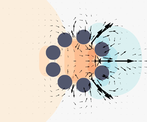
For all three phase differences, most of the cylinders push the surrounding fluid inwards during contraction, gradually increasing pressure  $p/\rho U_{max}^2$ inside the array ( $t^*=0$– $0.5$, i–iv in figure 8; see also supplementary movie 1). Because the cylinder array does not form a continuous boundary, the fluid inside the array tends to escape through the gaps from the contracting array, inducing a blowing flow out of the array. The blowing flow can be identified by the outward velocity vectors in figure 8(i–iv). At the same time, the generation of the gap flow between adjacent cylinders is affected by the size of the gaps. The gap flow is relatively extensive when the gap is large, assuming that other conditions, such as the directions of cylinder motion and pressure gradient across the gap, are similar. For $\Delta \phi ={\rm \pi} /5$ and ${\rm \pi} /15$ (figure 8a,b), the gaps on the right side of the array are generally wider than those on the left side during contraction, and thus the blowing flow is dominant on the right side of the array. For the subsequent expansion phase ( $t^*=0.5$– $1.0$), the expanding array sucks the surrounding fluid inwards by lowering the internal pressure (v–viii in figure 8). Opposite to the contraction phase, the gaps are wider on the left side of the array during expansion, making the suction flow prevalent on the left side of the array. As a result, for both the expansion phase and contraction phase, the overall gap flow is biased along the positive $x$ direction.

Figure 8. Snapshots of dimensionless pressure ( $p/\rho U_{max}^2$) contours and fluid velocity ( $\boldsymbol {u}/U_{max}$) vectors at eight instants with equal intervals during a cycle for phase difference $\Delta \phi _{{peak}} =$ (a) ${\rm \pi} /5$, (b) ${\rm \pi} /15$ and (c) $4{\rm \pi} /5$ ( $A=0.5$, $f=0.5$ and $Re=10$). The top row (i–iv) and bottom row (v–viii) show the contraction and expansion of the array, respectively. See supplementary movie 1 available at https://doi.org/10.1017/jfm.2023.1070.
Furthermore, by virtue of the high fluid viscosity and strong viscous diffusion, the boundary layer on the cylinder surface grows thick enough to overlap with the other boundary layer of the adjacent cylinder and forms a virtual fluid barrier in the gap, suppressing the penetration of fluid through the gap. This phenomenon of hydrodynamic blockage occurs between close solid structures in the low-Reynolds-number flow regime, and is a crucial mechanism for the propulsion and passive transport of tiny organisms with clustered appendages (Barta & Weihs Reference Barta and Weihs2006; Nawroth et al. Reference Nawroth, Feitl, Colin, Costello and Dabiri2010; Kolomenskiy et al. Reference Kolomenskiy, Farisenkov, Engels, Lapina, Petrov, Lehmann, Onishi, Liu and Polilov2020; Lee, Lee & Kim Reference Lee, Lee and Kim2020a; Lee et al. Reference Lee, Lee and Kim2020b; Kasoju & Santhanakrishnan Reference Kasoju and Santhanakrishnan2021; Lee & Kim Reference Lee and Kim2021). Consistent with the previous studies, it is reasonable to expect that the effect of the fluid barrier in this study is stronger for narrow gaps than for wide gaps. To confirm this, we compare the in-gap velocity profiles in figure 9, which presents the leftmost and rightmost sets of cylinders ( $i=0,3$) that have the largest phase difference $3\Delta \phi$ and thus the largest difference in gap size within one cycle. In the contraction phase with outward gap flows (i–iv in figure 9), the flow through the narrow gap produced by cylinder set $i=0$ is suppressed by the strong hydrodynamic blockage and has a flat velocity profile, while the gap flow at cylinder set $i=3$ on the opposite side with a larger gap continuously develops to a larger magnitude. As the array proceeds to the expansion phase with inward gap flows (v–viii in figure 9), the narrower gap produced by cylinder set $i=3$ forms a stronger fluid barrier and has a smaller velocity magnitude than that through the gap at cylinder set $i=0$. That is, in addition to the physical size of the gaps, the hydrodynamic blockage guides the fluid towards relatively wide gaps and enhances the directionally biased distribution of the gap flow.

Figure 9. Normalized velocity profiles  $u/U_{max}$ in the positive $x$ direction for gap flows passing through the leftmost cylinder set ( $i=0$, solid line) and the rightmost cylinder set ( $i=3$, dashed line) during a cycle ( $\Delta \phi _{{peak}} = {\rm \pi}/5$). The eight instants (i–viii) correspond to the snapshots in figure 8; panels (i–iv) for contraction and panels (v–viii) for expansion.
The velocity profile in figure 9 also shows that the fluid near the cylinder often moves in the direction opposite to that of the fluid near the centre of the gap. That is, the signs of the velocity are different between the two locations. This behaviour is because the fluid near the cylinder is affected by the thick shear layer attached to the cylinder and moves in the direction of cylinder motion, rather than following the primary direction of gap flow. For instance, when the array expands at  $t^*=0.5$–0.75, the cylinder set $i=0$ and fluid near the cylinders move outwards (negative $x$ direction), while the fluid near the centre of the gap is drawn inwards (positive $x$ direction) to fill the expanding space inside the array.
The phase difference and spatial variation in gap size are responsible for the temporal trends of  $C_T$ and $-F_{x,i}$ depicted in figure 7(a,b). To better understand the dynamics of cooperative array motion, the fluid forces acting on the cylinders are schematically depicted for several key frames in figure 10. As the x-directional force is mainly caused by the leftmost ( $i=0$) and rightmost ( $i=3$) cylinder sets, we only examine these two cylinder sets for the fluid forces. In figure 10(a) for the early stage of contraction, despite the leading inward motion of cylinder set $i=0$, the fluid forces acting on the two cylinder sets have relatively small differences in magnitude, as shown in figure 7(b). However, during the subsequent inward motion of cylinder set $i=3$ (figure 10b), cylinder set $i=3$ is strongly affected by the high internal pressure at the array centre which has been built up by the preceding inward motion of the other cylinders, and this cylinder set receives a relatively strong fluid force along the outward direction from the mutual interaction with the other cylinders. As a result, the overall magnitude of $-F_{x,i}$ acting on cylinder set $i=3$ exceeds that of cylinder set $i=0$, leading to negative $C_T$ for the entire cylinder array (figure 7a,b).

Figure 10. Prescribed cylinder velocity vectors (grey) and fluid force vectors (red) for each cylinder during (a,b) contraction and (c–e) expansion ( $\Delta \phi _{{peak}} = {\rm \pi}/5$). The fluid force vectors acting on the cylinder are only depicted for cylinder sets $i=0,3$ for simplicity.
Similar to the contraction phase, the expansion phase can be divided into a process of internal pressure change and a process in which the forces exerted on the rightmost cylinder set are affected by the internal pressure. In figure 10(c) for the early stage of expansion, the internal pressure at the array centre decreases and becomes lower than outside the array; this is clearly demonstrated in figure 8(a). The outward motion of cylinder set  $i=3$ is more strongly affected by the low pressure at the array centre because cylinder set $i=3$ moves outwards after the low pressure region has formed at the array centre (figure 10d). That is, cylinder set $i=3$ is subjected to a stronger fluid force along the inward direction from the mutual interaction with the other cylinders. The overall magnitude of $-F_{x,i}$ for cylinder set $i=3$ surpasses that of cylinder set $i=0$, yielding positive $C_T$ for the cylinder array (figure 7a,b).
According to figure 8(a,b), the pressure and velocity distributions of  $\Delta \phi ={\rm \pi} /15$ and ${\rm \pi} /5$ appear to be similar at each instant $t^*$, but the blowing and suction of $\Delta \phi ={\rm \pi} /15$ are not as spatially biased as those of the peak phase difference $\Delta \phi _{peak}={\rm \pi} /5$. For $\Delta \phi ={\rm \pi} /15$, the gap size difference between the left cylinder sets ( $i=0,1$) and the right cylinder sets ( $i=2,3$) is relatively minor throughout the cycle, and the flow is weakly biased over the cycle as a consequence. Although the internal pressure becomes strong at the late stage of contraction, the weakly biased gap flow yields smaller $\bar {C}_T$. However, when the phase difference is large (i.e. $\Delta \phi =4{\rm \pi} /5$), both the array motion and resultant gap flow are distinctly different from the previous two cases (figure 8c). Some adjacent cylinders move in opposite directions due to the large $\Delta \phi$, leading to minor changes in the internal area and pressure over a cycle. In addition, while the gap size changes gradually along the $x$ axis for the small phase differences ( $\Delta \phi ={\rm \pi} /5, {\rm \pi}/15$), the gap size changes abruptly at the large phase difference ( $\Delta \phi =4{\rm \pi} /5$). Due to the unorganized spatial distribution of gap sizes at the large phase difference, large gaps appear in the middle of the array and the fluid barrier is not effectively utilized. The generated flow cannot be guided into the gaps at either end, resulting in less biased flow. The minor change in the internal pressure, coupled with the unorganized gap distribution, causes a significant reduction in $\bar {C}_T$. In summary, thrust generation through coordinated motion requires a strongly biased gap flow over a cycle to produce a large time-averaged thrust, and the intensity of the biased flow is mainly determined by the non-uniformity of gap sizes, which originates from the phase difference.
3.2. Prediction of thrust generation using motion parameters
Using the relation between the formation of a spatially biased gap flow and thrust generation discussed in § 3.1, we construct a new parameter composed of several geometric variables through a simple scaling argument. This parameter captures the trend in the time-averaged thrust with respect to the phase difference. The biased gap flow can be quantified by the net volume rate of the gap flow that enters and exits the circular boundary of the array. Considering the mass conservation of incompressible fluids, the total flux of fluid expelled out or drawn in through the gaps is equal to the change in the internal area of the array. Thus, we express the total volume flux of suction and blowing as the time derivative of the internal area,  $\mathrm {d} S_{in}/\mathrm {d} t$. Here, the internal area $S_{in}$ is the area of the grey octagon depicted in figure 11(a). To normalize the rate of change in the internal area, an average rate of internal area change at $\Delta \phi = 0$ is used; for simplicity, the area is assumed to be circular. For $\Delta \phi = 0$, the area changes from a maximum of ${\rm \pi} (D/2+A)^2$ to a minimum of ${\rm \pi} (D/2-A)^2$ over half a period, $T/2$. The normalized rate is then $(\mathrm {d} S_{in}/\mathrm {d} t)/(4{\rm \pi} DA/T) =\mathrm {d} S^*_{in}/\mathrm {d} t^*$, where $S_{in}^* = S/(4{\rm \pi} DA)$. For the contraction phase, in which the rate of internal area change $\mathrm {d} S^*_{in}/\mathrm {d} t^*$ is negative, an outward gap flow is generated and the total volume flux of the outward gap flow is then quantified as $-\mathrm {d} S^*_{in}/\mathrm {d} t^*$. This quantity is closely related with the temporal change in pressure inside the internal area, as exemplified in the pressure contours of figure 8.

Figure 11. (a) Schematic showing outward unit normal vector  $\boldsymbol {n}_j$ and angle $\theta _j$ at the $j$th gap. (b) Time-averaged flux coefficient $\bar \beta$ with respect to phase difference $\Delta \phi$ ( $A=0.5$, $f=0.5$ and $Re=10$).
The velocity vectors in figure 8 show the amount and direction of the flow passing through the cylinder gaps, and indicate that the flux in the gap flow at each gap is affected by the size and orientation of the gap. The size of the  $j$th gap depicted in figure 11(a) is denoted as $G_j(t^*)$. We assume that the ratio of the flux across the $j$th gap to the total flux across the eight gaps is approximated as the ratio of the gap size for the $j$th gap, $G_j(t^*)/G_{tot}(t^*)$, where $G_{tot}(t^*)$ is the total gap size of the eight gaps at that instant. While this assumption is acceptable at the low Reynolds number with strong hydrodynamic blockage, it is invalid at the high Reynolds number, which is discussed in § 3.4. The dimensionless flux of each gap flow is then expressed as a product of the rate of change in the internal area and the gap ratio: $-\mathrm {d} S^*_{in}(t^*)/\mathrm {d} t^* \times G_j(t^*)/G_{tot}(t^*)$. To establish a relation between the biased gap flow and thrust generation, the degree of bias in the generated flow is quantified by the $x$-directional component of the flux in the gap flow. Considering the outward-facing normal vector $\boldsymbol {n}_j(t^*)$ of the $j$th gap, the $x$ component of the gap is $G_j(t^*) \cos \theta _j(t^*)$, where $\theta _j$ is the angle between the vector $\boldsymbol {n}_j$ and the $x$ axis. The $x$-directional flux of the flow is obtained by replacing $G_j(t^*)$ with $G_j(t^*) \cos \theta _j(t^*)$. A flux coefficient $\beta (t^*)$ is then given by summing the $x$-directional fluxes through all gaps:
 \begin{equation} \beta(t^*)=\sum_{j = 1}^{N_{gap}}-\frac{\mathrm{d}S^*_{in}(t^*)}{\mathrm{d}t^*}\frac{G_j(t^*) \cos \theta_j(t^*)}{G_{tot}(t^*)}, \end{equation}
where  $N_{gap}$ is the total number of gaps ( $N_{gap} = 8$). The sign and magnitude of $\beta (t^*)$ denote the direction and strength of the biased gap flow: positive when the net gap flow is along the positive $x$ direction and negative when the net gap flow is along the negative $x$ direction. Accordingly, the time-averaged value of $\beta$ over a cycle (i.e. time-averaged flux along the $x$ direction) is expected to be correlated with the time-averaged thrust coefficient $\bar {C}_T$ in (3.2).
To evaluate the time-averaged extent of the biased flow over a cycle, the time-averaged flux coefficient  $\bar \beta$ is considered:
 \begin{equation} \bar\beta = \int_{0}^{1}\beta(t^*)\,\mathrm{d}t^*. \end{equation}
Indeed,  $\bar \beta$ in figure 11(b) exhibits a very similar tendency to the time-averaged thrust coefficient $\bar {C}_T$ in figure 7(c). Near phase differences of $\Delta \phi =0$ and ${\rm \pi}$, both $\bar {C}_T$ and $\bar \beta$ are close to zero, and more importantly, the value of $\Delta \phi$ that maximizes $\bar \beta$ is ${\rm \pi} /5$, matching the optimal phase difference for $\bar {C}_T$. Negative values of $\bar \beta$ are also observed near $\Delta \phi =3{\rm \pi} /5$. According to the definition of $\bar \beta$, its negative value means that the array has wider gaps facing the negative $x$ direction during contraction, while during the expansion, wider gaps face the positive $x$ direction. This array motion is not ideal for thrust generation along the negative $x$ axis and, indeed, the magnitude of $\bar {C}_T$ corresponding to the negative $\bar \beta$ is very small albeit positive. Interestingly, with only time-dependent geometric variables ( $S_{in}$, $G_{tot}$, $G_j$ and $\theta _j$) in (3.3) and (3.4), which can be calculated from the input parameters without numerical simulations, the trend in the time-averaged thrust generation for the complex coordinated motion of the cylinder array can be successfully predicted.
On the one hand, the time-dependent  $\beta$ in (3.3) is insufficient to predict the instantaneous thrust generation of the cylinder array. For instance, $\beta$ is positive for both contraction and expansion phases, while the signs of $C_T$ in each phase are opposite to each other; see figure 17 in the Appendix. For the instantaneous thrust, the temporal change of the flow inside the array (inside the internal area depicted in figure 6) should be considered as well as the flow through the gaps (through the boundary of the internal area). On the other hand, $\beta$ does not account for the time-varying flow within the array, making it unable to predict the instantaneous thrust. However, because of the periodicity of cylinder motion and generated flow, the change of the flow within the array over a period is negligible. For this reason, while $\beta$ is not in accordance with $C_T$, its cycle-averaged value $\bar {\beta }$ is found to be correlated with the cycle-averaged thrust $\bar {C}_T$.
3.3. Effects of oscillation amplitude and frequency
In addition to the phase difference effects addressed in § 3.1, we analyse how thrust generation is affected by the oscillation amplitude  $A$ and frequency $f$ while maintaining the fluid kinematic viscosity unchanged. The amplitude ranges between $A = 0.1$ and 0.5 to prevent any collisions between the cylinders, which may occur for amplitudes exceeding $A = 0.5$. The frequency varies from $f = 0.25$ to 1.0.
When the amplitude varies in the range of  $A = 0.1$–0.5 for a fixed frequency $f = 0.5$, the time-averaged thrust coefficient $\bar {C}_T$ maintains a consistent trend with respect to the phase difference, having the maximal value near the phase difference $\Delta \phi = {\rm \pi}/5$, but it gradually increases with $A$ near $\Delta \phi = {\rm \pi}/5$; refer to figure 12(a-i). Specifically, for $\Delta \phi = {\rm \pi}/5$, $\bar {C}_T$ increases from 0.29 to 0.47 as $A$ increases from 0.1 to 0.5. The change in $\bar {C}_T$ is relatively minor, compared with the five times increase in $A$. This thrust increase is not solely due to the greater velocity of cylinders, which results in stronger flow velocity and pressure (in dimensional forms). The change in spacing of an array also contributes to thrust generation. In the radial oscillations of cylinders, the differences in gap sizes at a given time magnify as $A$ increases, which is crucial for enhancing the degree of bias in the generated gap flow. The effects of $A$ on the bias of the gap flow are described in figure 13(a–c) and supplementary movie 2. For a large amplitude ( $A = 0.5$), the differences in the gap sizes become more pronounced in the middle of contraction or expansion. Thus, the gap flow is stronger through the wider gap between the cylinder set $i = 3$ at $t^* = 0.25$ and the wider gap between the cylinder set $i = 0$ at $t^* = 0.75$, yielding notable spatial variations in the gap flows. Note that the dimensionless pressure $p/\rho U_{max}^2$ inside the array is the most significant for $A = 0.1$ (figure 13a–c). However, strong dimensionless internal pressure itself does not guarantee the greater thrust coefficient, and the bias of the gap flow should be also considered.

Figure 12. (a) Time-averaged thrust coefficient  $\bar {C}_T$ and (b) time-averaged flux coefficient $\bar {\beta }$ versus phase difference $\Delta \phi$ for (i) five oscillation amplitudes $A$ (
$A$ ( $\,f = 0.5$) and (ii) five oscillation frequencies $f$ (
$f$ ( $A = 0.5$).

Figure 13. Snapshots of dimensionless pressure ( $p/\rho U_{max}^2$) contours and fluid velocity vectors ( $\boldsymbol {u}/U_{max}$) in (i) the middle of contraction ( $t^* = 0.25$) and (ii) the middle of expansion ( $t^* = 0.75$) for (a–c) three amplitudes $A=0.1$, 0.3 and 0.5 ( $\,f = 0.5$) and (d–f) three frequencies $f=0.25$, 0.5 and 1.0 ( $A = 0.5$). The phase difference is $\Delta \phi ={\rm \pi} /5$. See supplementary movie 2 for panels (a–c) and movie 3 for panels (d–f).
The time-averaged flux coefficient  $\bar \beta$ behaves similarly to $\bar {C}_T$ in that it increases monotonically with $A$ near $\Delta \phi = {\rm \pi}/5$. In contrast to $\bar {C}_T$, $\bar \beta$ is simply proportional to $A$ at any phase difference because the rate of change in the internal area and the gap size ratios, which constitute the flow coefficient in (3.3), are directly affected by the change in $A$. Although $\bar \beta$ does not accurately quantify the extent of thrust change by the varying amplitude, it suggests that a cylinder array with a larger amplitude produces a more biased flow.
As the frequency  $f$ increases for a fixed amplitude $A = 0.5$, $\bar {C}_T$ rather decreases despite the increasing cylinder speed, according to figure 12(a-ii). With the fourfold increase in $f$ from 0.25 to 1.0, $\bar {C}_T$ decreases from 0.63 to 0.41. For the large $f$, the faster movement of the cylinder reduces the thickness of the boundary layer on the cylinder surface due to the weaker viscous diffusion, which reduces the strength of the virtual fluid barrier in narrow gaps. Thus, the flow generated by the array is not well guided to wide gaps for the higher $f$, and the gap flow through the narrowest gap becomes stronger than with the lower $f$. In figure 13(d–f) and supplementary movie 3, this result is clearly depicted by the sizes of arrows representing the dimensionless fluid velocity $\boldsymbol {u}/U_{max}$ in the narrow gaps. The weakened hydrodynamic blockage lowers the degree of bias in the gap flow and consequently decreases $\bar {C}_T$. It is noteworthy that $\bar {C}_T$ increases notably as $f$ changes from 0.375 to 0.25, while the variation in $\bar {C}_T$ is relatively minor in the range $f = 0.375$–1.0. The viscous diffusion length $\delta$ (i.e. boundary layer thickness) from a solid object generally scales as $\delta \sim (\nu /f)^{1/2}$ for oscillating flow and this scaling indicates non-uniform variation in $\delta$ with respect to $f$. For the low frequency of $f = 0.25$, the significant growth of viscous diffusion length eventually leads to the notable increase in $\bar {C}_T$.
As  $f$ varies for a given $A$, the configuration of the cylindrical array remains identical at a given dimensionless time $t^*$. The rate of change of the internal area in the dimensionless form, $\mathrm {d}S^*_{in}/\mathrm {d}t^*$, as well as the gap ratio $G_j(t^*)/G_{tot}(t^*)$ of each gap do not change at the given $t^*$. Consequently, the flux coefficient $\beta$ in (3.3) and the time-averaged flux coefficient $\bar {\beta }$ in (3.4) are independent of $f$; see figure 12(b-ii). This is because the flux coefficient is determined by the geometric characteristics of the array and does not account for the viscous effects of the fluid, which is responsible for the variation in $\bar {C}_T$ by $f$ (figure 12a-ii).
3.4. Thrust generation under different flow regimes
As the virtual fluid barrier that contributes to generating thrust is known to be effective in the low- $Re$ regime, we investigate the effect of viscosity on thrust generation. In addition to $Re=10$ considered thus far, $Re=5$ and $100$ are examined as the representatives of higher and lower viscosities, respectively. The motion parameters remain the same as in § 3.1 ( $A=0.5$ and $f=0.5$). No adjustments to the numerical settings were necessary for achieving convergence in the simulations with the changed Reynolds numbers; only a few additional iterations were required within each time step.
As the Reynolds number decreases from 10 to 5, the trend of thrust generation with respect to the phase difference remains similar, having the optimal phase difference at  $\Delta \phi = {\rm \pi}/5$, as shown in figure 14. The enhancement of thrust is also observed across most phase differences. This result is expected from the thrust-generating mechanism explained in § 3.1. Although the virtual fluid barrier is used to create a biased flow at both Reynolds numbers, flow penetrating through narrow gaps becomes more suppressed as viscosity increases. Instead, a significant amount of fluid prohibited by the narrow gaps passes through the wide gaps, thereby increasing the degree of bias in the gap flow and producing stronger thrust. Since the same hydrodynamic blockage mechanism applies for both $Re = 10$ and 5, hereafter, we will focus on examining how the disappearance of hydrodynamic blockage affects flow distribution and thrust by comparing $Re = 10$ and 100.

Figure 14. Time-averaged thrust coefficient  $\bar {C}_T$ for $Re=5, 10$ and $100$ ( $A=0.5$ and $f=0.5$).
When  $Re$ increases from 10 to 100, $\bar {C}_T$ decreases at all phase differences. Obviously, the high Reynolds number ( $Re=100$) produces a markedly different trend in $\bar {C}_T$ with respect to the phase difference $\Delta \phi$ compared with the low Reynolds numbers ( $Re=5$ and 10) (figure 14). The value of $\bar {C}_T$ reaches its maximum near $\Delta \phi ={\rm \pi} /15$ and drops sharply until $\Delta \phi ={\rm \pi} /5$, remaining low up to $\Delta \phi ={\rm \pi}$. With $\Delta \phi ={\rm \pi} /5$, in particular, $\bar {C}_T$ decreases from 0.47 to 0.046 (figure 14). For a single isolated cylinder model, as $Re$ increases from 10 to 100, the shear stress on the cylinder wall and the resultant viscous force acting on the cylinder are reduced because of the tenfold decrease in fluid viscosity. However, for our cylinder array, the reduction in the magnitude of the viscous force due to the lower fluid viscosity is not a primary reason for the remarkable decline in $\bar {C}_T$. Similar to increasing the frequency (§ 3.3, figure 12a-ii), the weaker thrust generation for $Re=100$ can be attributed to the decline in the hydrodynamic blockage; the increase in the frequency has the same effect as the increase in the Reynolds number. The viscous diffusion length of the boundary layer scales with the square root of the fluid kinematic viscosity (Schlichting & Gersten Reference Schlichting and Gersten2000; Nawroth et al. Reference Nawroth, Feitl, Colin, Costello and Dabiri2010). With a high Reynolds number ( $Re = 100$) and one-tenth of the kinematic viscosity, the boundary layer becomes notably thinner due to reduced viscous diffusion, causing the virtual fluid barrier in the gaps to almost disappear. The significantly weakened viscous diffusion and fluid barrier effect make the temporal variation in the internal pressure less distinct, and the gap flows generated through the narrow gaps are as strong as those through the wider gaps. This results in a decrease in the degree of bias in the gap flow; compare figure 15(a) with figure 15(b) and see supplementary movie 4.

Figure 15. Snapshots of dimensionless pressure contours ( $p/\rho U_{max}^2$) and fluid velocity vectors ( $\boldsymbol {u}/U_{max}$) in (i) the middle of contraction ( $t^* = 0.25$) and (ii) the middle of expansion ( $t^* = 0.75$) for (a) $Re = 10$ and (b) $Re = 100$ ( $A=0.5$, $f=0.5$ and $\Delta \phi ={\rm \pi} /5$). See supplementary movie 4.
The distinct trend of  $\bar {C}_T$ for $Re=100$ in figure 14 cannot be accurately captured using $\bar {\beta }$. This limitation arises because $\beta$ is based on the assumption that the virtual fluid barrier is sufficiently effective and does not directly reflect the variations in kinematic viscosity. The decrease in viscosity and weakened hydrodynamic blockage cause substantial changes in gap flow, and the basic assumption of $\beta$ that the flux through the gap is correlated with the gap size is no longer valid.
The weak fluid barrier for  $Re=100$ is identifiable from the large velocity vectors in the narrow gaps in figure 15(b), and is more apparent in the $x$-directional velocity profiles of gap flows presented in figure 16 for $\Delta \phi ={\rm \pi} /5$. As $Re$ increases from 10 to 100, the gap flow through the narrower gaps is enhanced in both the contraction and expansion phases. In the middle of contraction, at $t^* = 0.25$ (figure 16i), the gap at cylinder set $i = 0$ is narrower than that at $i =3$. By increasing $Re$ to 100, the magnitude of $u/U_{max}$ increases by a factor of 3.3 at the midpoint of the narrower gap. Similarly, in the middle of expansion, at $t^* = 0.75$ (figure 16ii), the gap at cylinder set $i=3$ is narrower than that of $i=0$, and the magnitude of $u/U_{max}$ increases by a factor of 2.5 at the midpoint of the narrower gap. In return, for both the contraction and expansion phases, the lower volume of flow is guided to the wider gap in the opposite side, causing the $u$-velocity profile to have a notable deficit near the midpoint of the wider gap. The magnitude of $u/U_{max}$ at the midpoint of the wider gap decreases from 2.84 to 0.68 at $t^* = 0.25$ and from 2.34 to 1.13 at $t^*=0.75$. As a result of the weaker hydrodynamic blockage effect, the magnitude of the instantaneous force acting on each cylinder decreases, although the shape of the temporal force profile over a cycle is retained. In summary, the lower level of viscous diffusion of the high-Reynolds-number flow hinders the fluid inside the array from exiting through the wider gap, eventually annihilating the bias of the gap flow and decreasing the time-averaged thrust.

Figure 16. Normalized velocity profiles  $u/U_{max}$ in the positive $x$ direction for gap flows passing through the leftmost cylinder set ( $i=0$, solid line) and the rightmost cylinder set ( $i=3$, dashed line) during a cycle; $Re = 10$ and 100. The velocity profiles are in (i) the middle of contraction ( $t^* = 0.25$) and (ii) the middle of expansion ( $t^* = 0.75$).
4. Concluding remarks
In this study, we have examined the thrust-generating strategy of a multi-body system in the low-Reynolds-number regime, using repeated suction and blowing through coordinated motion. The phase difference of the cylinders in the array is critical in producing asymmetric flow and consequently generating net thrust. The optimal phase difference that maximizes the time-averaged thrust exists, and is almost unaffected by changes in the oscillation amplitude and frequency. The flux coefficient for determining the strength and bias of the gap flow was constructed from the input parameters, with the assumption that the flux through the gap is correlated with the gap size. The trend of the time-averaged flux coefficient was found to be remarkably consistent with that of the time-averaged thrust coefficient at the low-Reynolds-number regime, enabling successful predictions of the optimal phase difference for the peak time-averaged thrust. As the Reynolds number increases, net thrust generation declines because the virtual fluid barrier is no longer effective. That is, for effective thrust generation, the hydrodynamic blockage produced by viscous diffusion in the gaps of the array should be accompanied by the coordinated suction and blowing of separate but close individual bodies.
Our preliminary multi-body model is limited to simple geometry and motions (circular cylinders with radial oscillations only) in a two-dimensional still fluid. Nevertheless, the proposed concept based on multiple separate bodies and hydrodynamic blockage can be easily extended to advanced flow-generating systems, which are more appropriate to actual environments; for example, the model moving in space collectively by imposing external input and generating thrust and flow. The multi-body system in the low-Reynolds-number flow possesses significantly reduced degrees of freedom owing to the discrete bodies and utilizes effective hydrodynamic blockage in the gaps between the bodies. By virtue of these advantages, the multi-body system with coordinated motion provides alternative solutions for small-scale propulsion, fluid transport and flow control based on particle clusters, replacing traditional continuous structures.
Supplementary movies
Supplementary movies are available at https://doi.org/10.1017/jfm.2023.1070.
Funding
This research was supported by the Basic Science Research Program through the National Research Foundation of Korea (NRF) funded by the Ministry of Science and ICT (NRF-2020R1A2C2102232).
Declaration of interests
The authors report no conflict of interest.
Appendix. Comparison of thrust coefficient and flux coefficient
The thrust coefficient  $C_T$ (3.1) and flux coefficient $\beta$ (3.3) of the cylinder array are compared in figure 17 for three values of the phase difference, $\Delta \phi ={\rm \pi} /15$, ${\rm \pi} /5$ and $4{\rm \pi} /5$.

Figure 17. Time histories of (a) thrust coefficient  $C_T$ and (b) flux coefficient β for three phase differences of $\Delta\phi={\rm \pi}/15$, ${\rm \pi}/5$ and $4{\rm \pi}/5$ ( $A=0.5$, $f=0.5$ and $Re=10$).


 Open access