


1. Introduction
Turbulent flows of a compressible viscous fluid are mostly described by the Navier–Stokes (NS) equations in the conservation form
 \begin{equation} \frac{\partial\boldsymbol{U}}{\partial t}+\boldsymbol{\nabla}\ \boldsymbol{\cdot}\ \boldsymbol{F}_a=\boldsymbol{\nabla}\ \boldsymbol{\cdot}\ \boldsymbol{F}_d, \end{equation}
subject to a given proper boundary condition and the initial condition
 \begin{equation} \boldsymbol{U}|_{t=0}=\boldsymbol{U}_0(\boldsymbol{r}), \quad \boldsymbol{r}\in\varOmega, \end{equation}
where  $\boldsymbol {U}(\boldsymbol {r},t)=(\rho,\rho \boldsymbol {u},E)^{\rm {T}}$ is a vector of conserved variables, $\boldsymbol {\nabla }$ is the Hamiltonian/ gradient operator,
 \begin{equation} \boldsymbol{F}_a= \begin{pmatrix} \rho\boldsymbol{u} \\ \rho\boldsymbol{u}\otimes\boldsymbol{u}+P\boldsymbol{\mathsf{I}} \\ (E+P)\boldsymbol{u} \end{pmatrix}, \quad \boldsymbol{F}_b= \begin{pmatrix} 0 \\ {\boldsymbol{\mathsf{\tau}}} \\ \boldsymbol{u}\ \boldsymbol{\cdot} \, {\boldsymbol{\mathsf{\tau}}}+\boldsymbol{q} \end{pmatrix} \end{equation}
are the advection/hyperbolic and diffusion fluxes,  $\boldsymbol {r}\in \varOmega$ is the vector of spatial position, $t$ denotes the time, $\boldsymbol {U}_0(\boldsymbol {r})$ is a given vector, $\rho$ is the density of mass, $\boldsymbol {u}$ is the velocity vector, $\boldsymbol {u}\otimes \boldsymbol {u}$ denotes the tensor product of $\boldsymbol {u}$ and $\boldsymbol {u}$, $P$ is the pressure, $\boldsymbol{\mathsf{I}}$ denotes the unit tensor, $E$ is the total energy per unit mass, $\boldsymbol{\mathsf{\tau}}$ denotes the tensor of viscous stress, and $\boldsymbol {q}$ is the vector of heat diffusion flux.
Note that tiny stochastic disturbances in fluid flows resulting from either small-scale thermal fluctuations or environmental noises are unavoidable in practice, and the triggered deviations might increase exponentially (Leith & Kraichnan Reference Leith and Kraichnan1972; Boffetta & Musacchio Reference Boffetta and Musacchio2001, Reference Boffetta and Musacchio2017). However, these tiny stochastic disturbances are not considered in the above-mentioned NS equations (1.1)–(1.3a,b) that are deterministic. Landau & Lifshitz (Reference Landau and Lifshitz1959) proposed a stochastic form of the NS equations that models the effect of thermal fluctuations via an additional stochastic stress tensor (Graham Reference Graham1974; Swift & Hohenberg Reference Swift and Hohenberg1977; Bell, Garcia & Williams Reference Bell, Garcia and Williams2007; Donev et al. Reference Donev, Vanden-Eijnden, Garcia and Bell2010, Reference Donev, Nonaka, Sun, Fai, Garcia and Bell2014). However, direct numerical simulations (DNS) of this stochastic model are rather difficult due to the extremely fine resolution that is required to measure accurately the velocities at dissipation-range length scales. By contrast, molecular dynamics provides molecular-level simulation techniques (Bird Reference Bird1998; Donev et al. Reference Donev, Bell, De la Fuente and Garcia2011; Smith Reference Smith2015; McMullen et al. Reference McMullen, Krygier, Torczynski and Gallis2022) for investigating directly the role of thermal fluctuations in turbulent flows.
Recently, McMullen et al. (Reference McMullen, Krygier, Torczynski and Gallis2022) investigated a decaying turbulent flow and found that, due to thermal fluctuations, the molecular gas dynamics spectra grow quadratically with wavenumber in the dissipation range, while the NS spectra decay exponentially. Furthermore, the transition to quadratic growth occurs at a length scale much larger than the gas molecular mean free path, namely in a regime that the NS equations are widely believed to describe. Thus they provided the first direct evidence that ‘the Navier–Stokes equations do not describe turbulent gas flows in the dissipation range because they neglect thermal fluctuations’ (McMullen et al. Reference McMullen, Krygier, Torczynski and Gallis2022), which is in agreement with the results given by Bandak et al. (Reference Bandak, Goldenfeld, Mailybaev and Eyink2022), Bell et al. (Reference Bell, Nonaka, Garcia and Eyink2022), Eyink & Jafari (Reference Eyink and Jafari2022), and others. Separately, Gallis et al. (Reference Gallis, Torczynski, Krygier, Bitter and Plimpton2021) used the direct simulation Monte Carlo (DSMC) method (molecular gas dynamics) and DNS of the NS equations to simulate a freely decaying turbulent flow, i.e. the compressible Taylor–Green vortex flow, and found that both methods produce basically the same energy decay for the Mach and Reynolds numbers that they examined, but the molecular fluctuations in DSMC (and in experiments) can break symmetries, which in turn can cause flows different from but basically similar to those given by DNS. Note that the above-mentioned investigations focus mainly on the influence of tiny stochastic disturbances resulting from thermal fluctuations on small-scale properties of freely decaying turbulence. Might the micro-level stochastic disturbances have huge influences on large-scale properties of some sustained turbulent flows? This is the primary motivation for our investigation in this paper.
Some turbulent flows might have multiple states according to Frisch (Reference Frisch1986), and his well-known monograph on turbulence (Frisch Reference Frisch1995) states that ‘it is typical for dissipative dynamical systems to have more than one attractor’ and ‘each attractor has an associated basin’, and thus ‘the statistical properties of the solution will then depend on to which basin the initial condition belongs’. The first evidence of this phenomenon in a turbulent flow is given by Huisman et al. (Reference Huisman, van der Veen, Sun and Lohse2014) in their study on the highly turbulent Taylor–Couette flow. Note that this work focuses mainly on the influence of initial data on the flow state of turbulence as well as its statistical properties. Considering that there are some previous investigations (Knobloch & Weiss Reference Knobloch and Weiss1989; Kraut, Feudel & Grebogi Reference Kraut, Feudel and Grebogi1999; Masoller Reference Masoller2002; de Souza et al. Reference de Souza, Batista, Caldas, Viana and Kapitaniak2007) into the effects of noises (in general whose levels are much larger than the stochastic disturbances considered later in this paper) on the dynamical systems with multiple attractors, in this paper we aim to demonstrate that not only the initial conditions but also the weak, small-scale stochastic noises/disturbances can determine in which basin the solution of a sustained turbulent flow will reside for a long time.
In theory, the influence of tiny stochastic disturbances on turbulent flows is fundamental, since this kind of stochastic disturbance is often in a micro-level of magnitude and is unavoidable in practice. There are two kinds of stochastic disturbance: natural and artificial. Thermal fluctuation belongs to the former, whereas the latter can be caused by many sources. Note that the background numerical noises, i.e. truncation errors and round-off errors, always exist for all numerical algorithms. Also, it is widely believed that turbulence has a close relationship with chaos, and thus the background numerical noises should increase exponentially (and quickly) up to the same level of ‘true’ physical solution. Therefore, a computer-generated simulation of the NS equations is a kind of mixture of the ‘true’ physical solution and ‘false’ numerical noises. Note that the background numerical noise is tiny and random, dependent on different numerical algorithms and data accuracy, which itself is a kind of artificial stochastic disturbance. Therefore, in a natural way, the background numerical noises can be regarded as the sum of all kinds of tiny artificial stochastic disturbances. In this paper, we investigate the large-scale influences of numerical noises as tiny artificial stochastic disturbances on a sustained turbulence by means of solving numerically the above-mentioned NS equations via a traditional numerical algorithm (the Runge–Kutta method with double precision, denoted RKwD) and the so-called ‘clean numerical simulation’ (CNS) (Liao Reference Liao2009, Reference Liao2013, Reference Liao2014; Hu & Liao Reference Hu and Liao2020; Qin & Liao Reference Qin and Liao2020; Li, Li & Liao Reference Li, Li and Liao2021; Xu et al. Reference Xu, Li, Li and Liao2021; Liao, Li & Yang Reference Liao, Li and Yang2022; Liao & Qin Reference Liao and Qin2022), separately, with the same initial/boundary conditions, using the same values of physical parameters. The result given by the traditional numerical algorithm RKwD is a mixture of the ‘true’ physical solution and ‘false’ numerical noises, which are mostly of the same order of magnitude, where the background numerical noise is regarded as the sum of all tiny artificial stochastic disturbances. By contrast, the CNS can greatly reduce the background numerical noise to any a required level so that the numerical noises are negligible compared with the ‘true’ physical solution, and thus the corresponding numerical result is convergent (reproducible) in an interval of time long enough for statistics, as described below. In other words, results given by the CNS can be regarded as a ‘clean’ benchmark solution. Thus we can investigate the influences of tiny artificial stochastic disturbances on turbulent flows by means of comparing the RKwD simulations with the CNS benchmark solution.
Let us discuss briefly the motivation and basic ideas of the CNS. Strictly speaking, all numerical simulations are not ‘clean’, since background numerical noises (i.e. truncation errors and round-off errors) always exist there. Indeed, for non-chaotic systems, the magnitude of numerical noises can be controlled on a tiny level much smaller than the ‘true’ physical solution so that the influences of the numerical noises can be neglected. However, for chaotic dynamical systems (Li & Yorke Reference Li and Yorke1975; Parker & Chua Reference Parker and Chua1989; Lorenz Reference Lorenz1993; Peter Reference Peter1998; Sprott Reference Sprott2010), numerical noises increase exponentially due to the ‘sensitivity dependence on initial condition’ (SDIC), which was first discovered by Poincaré (Reference Poincaré1890) and later rediscovered by Lorenz (Reference Lorenz1963) with the more famous name ‘butterfly effect’: a hurricane happening in North America might be created by a flapping of the wings of a distant butterfly in South America several weeks earlier. More importantly, it was further found by Lorenz (Reference Lorenz1989, Reference Lorenz2006) that a chaotic dynamical system has the sensitivity dependence not only on initial condition (SDIC) but also on numerical algorithms (SDNA) in single/double precision. This kind of uncertainty certainly raises serious doubt about the reliability of numerical simulations of chaotic systems. For example, Teixeira, Reynolds & Judd (Reference Teixeira, Reynolds and Judd2007) carefully investigated the time-step sensitivity of three nonlinear atmospheric models by means of some traditional numerical algorithms (in single/double precision), and made a rather pessimistic conclusion that ‘for chaotic systems, numerical convergence cannot be guaranteed forever’.
To overcome the above-mentioned limitations/restrictions of traditional numerical algorithms (in single/double precision) for chaotic dynamical systems, Liao (Reference Liao2009) suggested a numerical strategy, namely the ‘clean numerical simulation’ (CNS). The basic idea of the CNS (Liao Reference Liao2013, Reference Liao2014; Hu & Liao Reference Hu and Liao2020; Qin & Liao Reference Qin and Liao2020; Li et al. Reference Li, Li and Liao2021; Liao et al. Reference Liao, Li and Yang2022; Liao & Qin Reference Liao and Qin2022) is to greatly decrease the background numerical noises, i.e. truncation errors and round-off errors, to such a tiny level that the influence of numerical noises can be neglected in an interval of time  $0\leqslant t \leqslant T_{c}$ that is long enough for statistics, where $T_{c}$ is the so-called ‘critical predictable time’. The CNS is based on a well-known phenomenon: for a numerical/computer-generated simulation of a chaotic dynamical system, the level of simulation deviation (in an average meaning) from its (‘true’) physical solution increases exponentially to a macroscopic one (at $t = T_{c}$), i.e.
 \begin{equation} {\mathcal{E}}(t) = {\mathcal{E}}_0 \exp(Kt), \quad t\in[0, T_{c}], \end{equation}
where  $K > 0$ is the so-called ‘noise-growing exponent’, ${\mathcal {E}}_0$ denotes the level of background numerical noise, and ${\mathcal {E}}(t)$ is the level of simulation deviation (in an average meaning) from the physical solution. In theory, the critical predictable time $T_c$ is determined by a critical level ${\mathcal {E}}_c$ of simulation deviation from its physical solution, i.e.
 \begin{equation} T_{c} = \frac{1}{K} \ln \left( \frac{{\mathcal{E}}_c}{ {\mathcal{E}}_0 }\right). \end{equation}
Obviously, for a given critical level  ${\mathcal {E}}_c$, the smaller the level of the background numerical noise ${\mathcal {E}}_0$, the larger the critical predictable time $T_c$. This is the reason why in the frame of the CNS we have to greatly decrease the background numerical noises, i.e. truncation errors and round-off errors, to a tiny enough level. So, different from the Taylor series method, the key point of the CNS is the so-called ‘critical predictable time’ $T_c$ that determines a temporal interval $[0,T_c]$ in which the numerical simulations are ‘reliable’ and ‘clean’, since their ‘false’ numerical noises are much smaller than the ‘true’ physical solution and thus are negligible. For more details about the CNS, please refer to Liao (Reference Liao2009, Reference Liao2013, Reference Liao2014) and his co-authors (Hu & Liao Reference Hu and Liao2020; Qin & Liao Reference Qin and Liao2020; Li et al. Reference Li, Li and Liao2021; Xu et al. Reference Xu, Li, Li and Liao2021; Liao et al. Reference Liao, Li and Yang2022).
The CNS has been applied successfully to many chaotic dynamical systems. For example, by means of traditional numerical algorithms (in double precision), one can get convergent (i.e. reproducible) numerical simulations of the famous Lorenz equations in a rather short interval of time, i.e. approximately  $t\in [0,32]$. However, using the CNS, a convergent numerical simulation of the Lorenz equations was obtained first by Liao (Reference Liao2009) in $t\in [0,1000]$ and then by Liao & Wang (Reference Liao and Wang2014) in a much longer interval of time, i.e. $t\in [0, 10\,000]$. Also, since the background numerical noises of the CNS can be much smaller even than the micro-level physical uncertainty, Lin, Wang & Liao (Reference Lin, Wang and Liao2017) applied the CNS successfully to provide direct rigorous evidence that the micro-level thermal fluctuation is the origin of macroscopic randomness of the turbulent Rayleigh–Bénard convection (RBC). In particular, it is worth noting that the CNS has been applied successfully to find more than $2000$ new families of periodic orbits of three-body systems (Li & Liao Reference Li and Liao2017, Reference Li and Liao2019; Li, Jing & Liao Reference Li, Jing and Liao2018; Li et al. Reference Li, Li and Liao2021; Liao et al. Reference Liao, Li and Yang2022). The discovery of these new periodic orbits was reported twice in the famous popular magazine New Scientist (Crane Reference Crane2017; Whyte Reference Whyte2018), because only three families of periodic orbits of the three-body problem had been reported in three hundred years after Newton mentioned this problem in 1687. All of these illustrate the validity, novelty and great potential of the CNS.
Recently, an efficient CNS algorithm has been proposed to solve spatio-temporal chaotic systems, i.e. the complex Ginzburg–Landau equation (Hu & Liao Reference Hu and Liao2020) and the damped driven sine-Gordon equation (Qin & Liao Reference Qin and Liao2020). Using the CNS result as a benchmark solution, one can investigate the influence of numerical noises on the computer-generated simulation of a spatio-temporal chaotic system. It was found (Hu & Liao Reference Hu and Liao2020; Qin & Liao Reference Qin and Liao2020) that numerical noises might lead to huge deviations of computer-generated simulations of some spatio-temporal chaotic systems, not only in trajectories but also even in statistics.
In this paper, we apply the CNS and a traditional algorithm (based on the fourth-order Runge–Kutta method with double precision, denoted RKwD), separately, to solve a sustained turbulence, i.e. the two-dimensional (2-D) turbulent RBC. Note that using the CNS, the background numerical noises can be decreased to such a tiny level that the numerical noises are negligible in a long enough interval of time, so that the CNS result can be regarded as a benchmark solution of the ‘true’ physical result to investigate the influence of tiny artificial stochastic disturbances by comparing the RKwD simulations with the CNS benchmark solution. In this way, we provide rigorous evidence that tiny artificial stochastic disturbances have huge influences on large-scale properties of the turbulent RBC not only in statistics but also even in flow types. The CNS benchmark solution always keeps the vortical/roll-like turbulent convection; however, for the RKwD simulations, the shearing convection occurs and its corresponding flow field turns to zonal flow thereafter. This phenomenon is reasonable if the boundaries of different attractor basins (mentioned above) in this multistable system are intricately interwoven, as has been observed in other cases (Shrimali et al. Reference Shrimali, Prasad, Ramaswamy and Feudel2008).
2. Mathematical model for 2-D turbulent RBC
The buoyancy-driven convection in a fluid layer between two horizontal parallel plates heated from below and cooled from above, known as the RBC for compressible viscous fluids, is one of the most fundamental and classic paradigms of nonlinear dynamics in fluid mechanics. It was first investigated by Rayleigh (Reference Rayleigh1916), and the continuous efforts devoted to the study of this problem have greatly enriched our understanding (Chandrasekhar Reference Chandrasekhar1961; Schlüter, Lortz & Busse Reference Schlüter, Lortz and Busse1965; Heslot, Castaing & Libchaber Reference Heslot, Castaing and Libchaber1987; Kadanoff Reference Kadanoff2001; Niemela & Sreenivasan Reference Niemela and Sreenivasan2006; Ahlers, Grossmann & Lohse Reference Ahlers, Grossmann and Lohse2009; Lohse & Xia Reference Lohse and Xia2010; Zhou & Xia Reference Zhou and Xia2013; Goluskin et al. Reference Goluskin, Johnston, Flierl and Spiegel2014; Wang et al. Reference Wang, Chong, Stevens, Verzicco and Lohse2020).
As illustrated in figure 1, a thin layer of fluid is confined between two horizontal plates that are separated by a distance  $H$, where $T_{0}$ and $T_{0}+\Delta T$ denote the temperatures of the top and bottom boundary surfaces, respectively, $L$ is the horizontal length of the computational domain, and $g$ is the gravity acceleration. The typical vortical/roll-like motions of 2-D RBC, as illustrated in figure 1(a), and their corresponding turbulent states, have been studied extensively by means of DNS (Saltzman Reference Saltzman1962; Fromm Reference Fromm1965; Veronis Reference Veronis1968; Moore & Weiss Reference Moore and Weiss1973; Curry et al. Reference Curry, Herring, Loncaric and Orszag1984; Zienicke, Seehafer & Feudel Reference Zienicke, Seehafer and Feudel1998; Johnston & Doering Reference Johnston and Doering2009; Huang & Zhou Reference Huang and Zhou2013; Zhang, Zhou & Sun Reference Zhang, Zhou and Sun2017; Zhu et al. Reference Zhu, Mathai, Stevens, Verzicco and Lohse2018). However, there is another type of flow in the 2-D turbulent RBC in the case of the free-slip boundary conditions imposed on two horizontal parallel plates and the periodic boundary conditions on the left and right sides, namely zonal flow (Goluskin et al. Reference Goluskin, Johnston, Flierl and Spiegel2014; van der Pol et al. Reference van der Pol, Ostilla-Mónico, Verzicco and Lohse2014; von Hardenberg et al. Reference von Hardenberg, Goluskin, Provenzale and Spiegel2015; Wang et al. Reference Wang, Chong, Stevens, Verzicco and Lohse2020), as shown in figure 1(b). It is worth noting that such a turbulent zonal flow has been widely found in nature and the laboratory, such as in the atmosphere of Jupiter (Heimpel, Aurnou & Wicht Reference Heimpel, Aurnou and Wicht2005; Kaspi et al. Reference Kaspi, Galanti, Hubbard, Stevenson, Bolton, Iess, Guillot, Bloxham, Connerney and Cao2018) and some Jovian planets (Sun, Schubert & Glatzmaier Reference Sun, Schubert and Glatzmaier1993; Cho & Polvani Reference Cho and Polvani1996; Yano, Talagrand & Drossart Reference Yano, Talagrand and Drossart2003), in the oceans (Maximenko, Bang & Sasaki Reference Maximenko, Bang and Sasaki2005; Richards et al. Reference Richards, Maximenko, Bryan and Sasaki2006), in the Earth's outer core (Miyagoshi, Kageyama & Sato Reference Miyagoshi, Kageyama and Sato2010), in toroidal tokamak devices (Diamond et al. Reference Diamond, Itoh, Itoh and Hahm2005), and so on. Thus here we choose the 2-D turbulent RBC with free-slip boundary conditions at the upper and lower plates, and periodic boundary conditions in the horizontal direction, as our mathematical model for the sustained turbulence, governed by the NS equations.

Figure 1. Schematic drawings of 2-D turbulent RBC in two totally different flow types: (a) typical vortical/roll-like flow, and (b) zonal flow. The fluid layer between two parallel plates that are separated by a height  $H$ obtains heat from the bottom boundary surface because of the constant temperature difference $\Delta T>0$, where $L$ is the horizontal length of the computational domain, and the downward direction of gravity acceleration $g$ is indicated.
Using the length scale  $H$, velocity scale $\sqrt {g\alpha H\,\Delta T}$ and temperature scale $\Delta T$ as the characteristic scales, the corresponding dimensionless NS equations, combined with the Boussinesq approximation (Saltzman Reference Saltzman1962), read
 $$\begin{gather} \frac{\partial}{\partial t}\nabla^{2}\psi+\frac{\partial(\psi,\nabla^{2}\psi)}{\partial(x,z)}-\frac{\partial\theta}{\partial x}-\sqrt{\frac{Pr}{Ra}}\,\nabla^{4}\psi=0, \end{gather}$$
 $$\begin{gather}\frac{\partial\theta}{\partial t}+\frac{\partial(\psi,\theta)}{\partial(x,z)}-\frac{\partial\psi}{\partial x}-\frac{1}{\sqrt{Pr\,Ra}}\,\nabla^{2}\theta=0, \end{gather}$$
where  $\psi$ is a stream function with the definition
 \begin{equation} u={-}\frac{\partial\psi}{\partial z}, \quad w=\frac{\partial\psi}{\partial x}, \end{equation}
in which  $u$ and $w$ are the horizontal and vertical velocities, $\theta$ is the temperature departure from a linear variation background (i.e. the temperature is expressed as $T=\theta -z+1$ in the case of $T_0=0$), $t$ denotes the time, $x\in [0,\varGamma ]$ and $z\in [0,1]$ are the horizontal and vertical position coordinates, $\varGamma =L/H$ denotes the aspect ratio, and $\nabla ^{2}$ is the Laplace operator, thus $\nabla ^{4}=\nabla ^{2}\nabla ^{2}$. Also,
 \begin{equation} \frac{\partial(a,b)}{\partial(x,z)}=\frac{\partial a}{\partial x}\frac{\partial b}{\partial z}-\frac{\partial b}{\partial x}\frac{\partial a}{\partial z} \end{equation}
is the Jacobi operator, and the Rayleigh number  $Ra$ and Prandtl number $Pr$ are defined by
 \begin{equation} Ra=\frac{g\alpha H^{3}\,\Delta T}{\nu\kappa}, \quad Pr=\frac{\nu}{\kappa}, \end{equation}
respectively, in which  $\alpha$ is the thermal expansion coefficient, and $\nu =\mu /\rho$ is the kinematic viscosity.
Note that free-slip boundary conditions are adopted at the upper and lower plates where temperatures are assumed to be constant. Hence the NS equations (2.1)–(2.2) have the following boundary conditions:
 \begin{equation} \psi=\frac{\partial^{2}\psi}{\partial z^{2}}=\theta=0 \end{equation}
at  $z=0$ and $z=1$. On the other hand, since the fluid layer can extend to infinity in the horizontal direction, we adopt the periodic boundary conditions for $\psi$ and $\theta$ at the lateral boundaries in the horizontal direction, i.e. at $x=0$ and $x = \varGamma$.
Without loss of generality, in this paper let us consider the case with aspect ratio  $\varGamma =L/H=2\sqrt {2}$, which is large enough for the approximation of heat flux at an infinite aspect ratio (Saltzman Reference Saltzman1962; Curry et al. Reference Curry, Herring, Loncaric and Orszag1984; Lin et al. Reference Lin, Wang and Liao2017), Prandtl number $Pr=6.8$ (corresponding to water at room temperature, $20\,^{\circ }{\rm C}$), and Rayleigh number $Ra=6.8\times 10^{8}$ (corresponding to a turbulent state). In addition, the initial temperature and velocity fields are generated randomly by the thermal fluctuations in Gaussian white noises (Lin et al. Reference Lin, Wang and Liao2017), with temperature standard deviation $\sigma _T=10^{-10}$ and velocity standard deviation $\sigma _u=10^{-9}$.
3. Influence of numerical noises as artificial stochastic disturbances
The deterministic NS equations (2.1)–(2.2) are solved numerically here, separately, by means of the traditional algorithm RKwD whose numerical noises are mostly of the same order of magnitude as the ‘true’ physical solution, and the CNS whose numerical noises are much less than the physical solution and thus are negligible. By means of comparing the RKwD simulations with the CNS benchmark solution, it is found that the numerical noises indeed might lead to huge large-scale differences even in statistics and flow types of the 2-D turbulent RBC, as described below.
First, we apply the CNS to greatly decrease the background numerical noises, i.e. the truncation errors and round-off errors, to such a tiny level that the numerical noises are much smaller than, and thus negligible compared with, the ‘true’ physical solution of the 2-D turbulent RBC in an interval of time that is long enough for statistics. In this way, a convergent (reproducible) solution of the 2-D turbulent RBC can be obtained, which is used here as the ‘clean’ benchmark solution. On the other hand, with the same initial/boundary conditions and the same physical parameters as described in the previous section, the NS equations (2.1)–(2.2) are also solved numerically by a traditional algorithm, i.e. RKwD, using the time step  $\Delta t = 1\times 10^{-4}$, whose numerical noises increase exponentially up to the same level of the ‘true’ physical solution and thus are not negligible. By comparing these RKwD simulations with the CNS benchmark solution, we can investigate in detail the influence of the numerical noises as tiny artificial stochastic disturbances on the 2-D turbulent RBC. In this section, we show only briefly some results for comparison. For details about the CNS algorithms, please refer to Appendix A.
Briefly speaking, to decrease the spatial truncation error to a small enough level, we discretize the spatial domain of flow field by a uniform mesh  $N_x\times N_z =1024\times 1024$, and also apply the Fourier spectral method with the $3/2$ rule for dealiasing (Pope Reference Pope2001). The corresponding spatial resolution is high enough for the considered turbulent RBC: the horizontal (maximum) grid spacing $\varDelta _x=L/N_x=0.00276$ is less than the minimum Kolmogorov scale (Pope Reference Pope2001), which will be shown later in detail. Also, to decrease the temporal truncation error to a small enough level for the CNS, we use the 45th-order (i.e. $M=45$) Taylor expansion with time step $\Delta t=10^{-3}$. In addition, to decrease the round-off error to a small enough level, we use 70 significant digits (i.e. $N_{s}=70$) in multiple precision for all physical/numerical variables and parameters. Similarly, we get another CNS result using the Fourier spectral method on the same uniform mesh $N_x\times N_z =1024\times 1024$ with even smaller background numerical noises by means of a higher-order (i.e. $M=47$) Taylor expansion with the same time step ( $\Delta t=10^{-3}$) and the higher multiple precision with more significant digits (i.e. $N_{s}=72$). Comparing these two CNS results, it is found that they have no distinct differences in an interval of time $0 \leqslant t\leqslant 500$, which is long enough for statistics. This verifies the convergence and reliability of our CNS result in $t\in [0,500]$ given by means of $M=45$, $\Delta t=10^{-3}$ and $N_{s}=70$, which is therefore used below as the ‘clean’ benchmark solution.
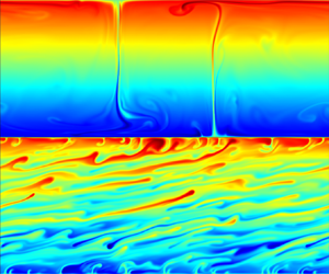
As shown in figures 2 and 3, the numerical simulation given by RKwD is compared with the ‘clean’ benchmark solution given by the CNS; see the supplementary movie available at https://doi.org/10.1017/jfm.2022.710. Note that these two simulations have exactly the same initial conditions caused by the micro-level thermal fluctuations. For both the CNS and RKwD simulations, the tiny initial disturbances of velocity and temperature evolve progressively from micro-level to macro-level until  $t\approx 25$, when the transition from laminar flow to turbulence occurs, then the strong mixing occurs in $t\in [25,36]$, and the typical vortical/roll-like convection appears at $t\approx 50$, as shown in figure 2. Thereafter, as the time increases, the RKwD simulation deviates from the CNS benchmark solution more and more, so that a distinct large-scale difference between them can be observed, indicating that the numerical noises (as artificial stochastic disturbances) could indeed lead to some large-scale differences of flow fields of velocity and temperature at a macroscopic level, for example, as shown in figure 2 at $t=100$ and $t=185$. However, even so, the flow type of these two simulations stays the same (i.e. vortical/roll-like turbulent convection) until $t\approx 188$, when the shearing convection occurs for the RKwD simulation and its corresponding flow field turns to a kind of zonal flow thereafter, as shown in figures 2 and 3. On the contrary, the CNS benchmark solution thereafter always sustains the non-shearing vortical/roll-like convection during the whole process of simulation. Therefore, the RKwD simulation and the CNS benchmark solution have different types of turbulent convection after $t>188$. It should be emphasized that such a qualitative large-scale difference is triggered only by the numerical noises (as artificial stochastic disturbances). All of these highly suggest that the numerical noises (as artificial stochastic disturbances) have quantitatively and qualitatively large-scale influences on the sustained turbulence, i.e. the 2-D turbulent RBC considered in this paper.

Figure 2. Evolutions of the  $\theta$ (dimensionless temperature departure from a linear variation background) field in the case $Pr = 6.8$, $Ra = 6.8 \times 10^{8}$ and $L/H = 2\sqrt {2}$: (a,c,e,g,i,k,m,o) the CNS benchmark solution; (b,d,f,h,j,l,n,p) the RKwD simulation using $\Delta t = 10^{-4}$. See the supplementary movie.

Figure 3. More evolutions of the  $\theta$ (dimensionless temperature departure from a linear variation background) field in the case $Pr = 6.8$, $Ra = 6.8 \times 10^{8}$ and $L/H = 2\sqrt {2}$: (a,c,e,g,i,k,m,o) the CNS benchmark solution; (b,d,f,h,j,l,n,p) the RKwD simulation using $\Delta t = 10^{-4}$. See the supplementary movie.
How about the influence of numerical noises (as artificial stochastic disturbances) on statistical results? The heat transport of 2-D turbulent RBC can be quantified typically by the Nusselt number defined by
 \begin{equation} Nu(t)=1-\left. \frac{\partial\langle\theta(x,z,t)\rangle_{x}}{\partial z}\right|_{z=1}, \end{equation}
where  $\langle a \rangle _{x}=\int _{0}^{\varGamma }a \,{{\rm d}\kern0.7pt x}/\varGamma$ denotes the spatial average in the horizontal direction. As shown in figure 4(a), the distinct deviation between the two time histories of $Nu(t)$ given respectively by the CNS benchmark solution and the RKwD simulation happens at $t\approx 80$ when the numerical noises of the RKwD simulation have been enlarged to a macroscopic level because of the butterfly effect of chaos. Note that the $Nu(t)$ given by the RKwD simulation drops down greatly at $t\approx 188$ until $Nu(t) \approx$ 30 after $t>300$, one order of magnitude less than that of the CNS benchmark solution. Such a huge difference is not only quantitative but also qualitative, which is definitely due to the appearance of the zonal flow at $t \approx 188$ that is triggered by the numerical noises of the RKwD simulation (as artificial stochastic disturbances). On the other hand, the Reynolds number is also calculated to measure the global convection strength, which is obtained via the root-mean-square (r.m.s.) velocity $U_{rms}$ (Sugiyama et al. Reference Sugiyama, Calzavarini, Grossmann and Lohse2009; Zhang et al. Reference Zhang, Zhou and Sun2017), i.e.
 \begin{equation} Re(t)=\sqrt{\frac{Ra}{Pr}}\,U_{rms}, \end{equation}
with  $U_{rms}=\sqrt {\langle u^2+w^2\rangle _{A}}$, where $\langle a\rangle _{A}=\int _{0}^{\varGamma }\int _{0}^{1}a\,{\rm d}\kern0.7pt x\,{\rm d}z/\varGamma$ denotes the spatial average. As shown in figure 4(b), the CNS benchmark solution and RKwD simulation give almost the same values of $Re(t)$ when $t < 188$. However, the departure begins at $t \approx 188$ when the shearing convection occurs, and thereafter the deviation between the RKwD simulation and the CNS benchmark solution becomes more and more obvious. Here, it should be emphasized that the Reynolds number $Re$ of the CNS benchmark solution at $t=500$ is about 3500 times larger than that of the RKwD simulation! This is indeed a huge difference. Similar phenomena are observed in the comparisons of the spatially averaged heat flux $\langle wT\rangle _{A}$ and kinetic energy $\langle E_V\rangle _{A}$, given respectively by the CNS benchmark solution and RKwD simulation, as shown in figures 5(a) and 5(b), where the maximum ratio of kinetic energy reaches about 2.5. Indeed, the numerical noises (as artificial stochastic disturbances) might lead to qualitatively huge deviations of the 2-D turbulent RBC.

Figure 4. Comparisons of the instantaneous Nusselt number  $Nu$ and Reynolds number $Re$ in the case $Pr = 6.8$, $Ra = 6.8 \times 10^{8}$ and $L/H = 2\sqrt {2}$: (a) the Nusselt number $Nu$; (b) the Reynolds number $Re$. Solid line in red denotes the CNS benchmark solution; dashed line in black denotes the RKwD simulation using $\Delta t = 10^{-4}$.

Figure 5. Comparisons of the spatially averaged heat flux  $\langle wT\rangle _{A}$ and kinetic energy $\langle E_V\rangle _{A}$ in the case $Pr = 6.8$, $Ra = 6.8 \times 10^{8}$ and $L/H = 2\sqrt {2}$, where $\langle a\rangle _{A}=\int _{0}^{\varGamma } \int _{0}^{1}a\,{\rm d}\kern0.7pt x\,{\rm d}z/\varGamma$ denotes the spatial average: (a) the heat flux $\langle wT\rangle _{A}$; (b) the kinetic energy $\langle E_V\rangle _{A}$. Solid line in red denotes the CNS benchmark solution; dashed line in black denotes the RKwD simulation using $\Delta t = 10^{-4}$.
Besides the above-mentioned large-scale quantities, the comparisons of some small-scale properties of fluid flows such as the kinetic energy dissipation rate  $\langle \varepsilon _{V}\rangle _{A}$ and the thermal dissipation rate $\langle \varepsilon _{T}\rangle _{A}$ of this 2-D turbulent RBC given by the CNS solution and the RKwD simulation are as shown in figure 6, where
 \begin{equation} \varepsilon_{V}(x,z,t)=\frac{1}{2}\sqrt{\frac{Pr}{Ra}}\sum_{ij}\left[ \partial_iu_j(x,z,t)+\partial_ju_i(x,z,t) \right]^2 \end{equation}
and
 \begin{equation} \varepsilon_{T}(x,z,t)=\frac{1}{\sqrt{Pr\,Ra}} \left| \boldsymbol{\nabla }\left[ \theta(x,z,t)-z \right] \right|^2, \end{equation}
with  $i$,
$i$,  $j=1,2$, $u_1(x,z,t)=u(x,z,t)$, $u_2(x,z,t)=w(x,z,t)$, $\partial _1=\partial /\partial x$, $\partial _2=\partial /\partial z$. Here, $\boldsymbol {\nabla }$ is the Hamiltonian operator, and $\langle \, \rangle _{A}$ denotes the spatial average. Note that for the RKwD simulation, both the kinetic energy dissipation rate $\langle \varepsilon _{V}\rangle _{A}$ and the thermal dissipation rate $\langle \varepsilon _{T}\rangle _{A}$ greatly drop down at $t\approx 188$ when the shearing convection (i.e. the zonal flow) occurs, which is triggered only by the numerical noises (as artificial stochastic disturbances).

Figure 6. Comparisons of the spatially averaged kinetic energy dissipation rate  $\langle \varepsilon _{V}\rangle _{A}$ and thermal dissipation rate $\langle \varepsilon _{T}\rangle _{A}$ in the case $Pr = 6.8$, $Ra = 6.8 \times 10^{8}$ and $L/H = 2\sqrt {2}$, where $\langle a\rangle _{A}=\int _{0}^{\varGamma }\int _{0}^{1}a\,{\rm d}\kern0.7pt x\,{\rm d}z/ \varGamma$ denotes the spatial average: (a) the kinetic energy dissipation rate $\langle \varepsilon _{V}\rangle _{A}$; (b) the thermal dissipation rate $\langle \varepsilon _{T}\rangle _{A}$. Solid line in red denotes the CNS benchmark solution; dashed line in black denotes the RKwD simulation using $\Delta t = 10^{-4}$.
By the way, as shown in figure 6(a), we have the maximum kinetic energy dissipation rate  $(\langle \varepsilon _{V}\rangle _{A})_{max}=0.00646$ at $t=26.9$ when the transition from the laminar flow to turbulence occurs, corresponding to the minimum Kolmogorov scale
 \begin{equation} \left(\langle\eta\rangle_{A}\right)_{min}\approx(Pr/Ra)^{3/8} \left[ (\langle\varepsilon_{V}\rangle_{A})_{max} \right] ^{{-}1/4}=0.00353. \end{equation}
Thus the criterion on the maximum horizontal grid spacing  $\varDelta _x=\varGamma /N_x=0.00276 < 0.8(\langle \eta \rangle _{A})_{min}=0.00282$ is indeed satisfied, so the spatial resolution used in this paper is fine enough for the 2-D turbulent RBC under consideration.
Figure 7 shows comparisons of the kinetic energy dissipation rate  $\langle \varepsilon _{V}\rangle _{x,t}(z)$ and the heat flux $\langle wT\rangle _{x,t}(z)$, where $\langle a\rangle _{x,t}=\int _{0}^{\varGamma }\int _{0}^{500}a \,{\rm d}\kern0.7pt x\,{\rm d}t/\varGamma /500$ denotes the horizontally spatial and temporal average. Obviously, both the kinetic energy dissipation rate $\langle \varepsilon _{V}\rangle _{x,t}$ and the heat flux $\langle wT\rangle _{x,t}$ of the CNS benchmark solution are significantly larger than those given by the RKwD simulation. In particular, near the lower and upper plates, $\langle \varepsilon _{V}\rangle _{x,t}$ given by the CNS benchmark solution has a much sharper peak than that given by the RKwD simulation, as shown in figure 7(a). This indicates that the numerical noises (as artificial stochastic disturbances) can lead to large-scale deviations in statistics of the 2-D turbulent RBC under consideration.

Figure 7. Comparisons of the horizontally and temporally averaged kinetic energy dissipation rate  $\langle \varepsilon _{V}\rangle _{x,t}(z)$ and the heat flux $\langle wT\rangle _{x,t}(z)$ in the case $Pr = 6.8$, $Ra = 6.8 \times 10^{8}$ and $L/H = 2\sqrt {2}$, where $\langle a\rangle _{x,t}=\int _{0}^{\varGamma }\int _{0}^{500}a\,{\rm d}\kern0.7pt x\,{\rm d}t/\varGamma /500$ denotes the horizontal and temporal average: (a) the kinetic energy dissipation rate $\langle \varepsilon _{V}\rangle _{x,t}(z)$; (b) the heat flux $\langle wT\rangle _{x,t}(z)$. Solid line in red denotes the CNS benchmark solution; dashed line in black denotes the RKwD simulation using $\Delta t = 10^{-4}$.
The comparison of the probability density functions (p.d.f.s) of the stream function  $\psi (x,z,t)$ in $0 \leqslant x < \varGamma$, $0 \leqslant z \leqslant 1$ and $0 \leqslant t \leqslant 500$ given by the CNS benchmark solution and the RKwD simulation is as shown in figure 8. Unlike the p.d.f. of the CNS benchmark solution that has a kind of asymmetry about $\psi = 0$, the p.d.f. of the RKwD simulation has no such kind of asymmetry but two peaks at $\psi \approx 0$ and $\psi \approx 0.25$. Furthermore, the comparison of the p.d.f.s of $\theta (x,z,t)$ given by the CNS benchmark solution and RKwD simulation is as shown in figure 9. As shown in figure 9(a), except at $\theta \approx 0$, the p.d.f. of $\theta (x,z,t)$ given by the CNS benchmark solution remains at almost the same value. In contrast, the p.d.f. of $\theta$ given by the RKwD simulation is relatively more typical, as shown in figure 9(b). Thus the numerical noises (as artificial stochastic disturbances) indeed lead to large-scale deviations even in the p.d.f.s of the 2-D turbulent RBC under consideration.

Figure 8. Probability density functions (p.d.f.s) of  $\psi (x,z,t)$ in $0 \leqslant x < \varGamma$, $0 \leqslant z \leqslant 1$ and $0 \leqslant t \leqslant 500$ in the case $Pr = 6.8$, $Ra = 6.8 \times 10^{8}$ and $L/H = 2\sqrt {2}$: (a) the p.d.f. given by the CNS benchmark solution; (b) the p.d.f. given by the RKwD simulation using $\Delta t = 10^{-4}$.

Figure 9. Probability density functions (p.d.f.s) of  $\theta (x,z,t)$ in $0 \leqslant x < \varGamma$, $0 \leqslant z \leqslant 1$ and $0 \leqslant t \leqslant 500$ in the case $Pr = 6.8$, $Ra = 6.8 \times 10^{8}$ and $L/H = 2\sqrt {2}$: (a) the p.d.f. given by the CNS benchmark solution; (b) the p.d.f. given by the RKwD simulation using $\Delta t = 10^{-4}$.
All of the above-mentioned comparisons indicate that the micro-level background numerical noises as a kind of artificial stochastic disturbances can lead to large-scale differences not only in spatio-temporal trajectories but also even in flow types of the 2-D turbulent RBC, which further affects the statistics of the Nusselt number, the Reynolds number, the kinetic energy, the kinetic energy dissipation rate, the thermal dissipation rate, and so on. Note that it is currently reported by McMullen et al. (Reference McMullen, Krygier, Torczynski and Gallis2022) that ‘the Navier–Stokes equations do not describe turbulent gas flows in the dissipation range because they neglect thermal fluctuations’; that is, tiny stochastic disturbances resulting from thermal fluctuations might influence the small-scale properties of the freely decaying turbulent flows under their consideration. In this paper, the detailed comparisons between the CNS benchmark solution and the RKwD simulation provide us with the rigorous evidence that numerical noises as a kind of small-scale artificial stochastic disturbances might influence the large-scale properties of a sustained turbulence, i.e. the 2-D turbulent RBC considered in this paper.
4. Concluding remarks and discussions
All numerical algorithms have background numerical noises, i.e. truncation errors and round-off errors, which are tiny and random. It was reported that for a chaotic dynamic system, random numerical noises increase exponentially due to the butterfly effect of chaos, up to the same order of magnitude as its ‘true’ physical solution (Hu & Liao Reference Hu and Liao2020; Qin & Liao Reference Qin and Liao2020). Therefore, numerical simulations of a deterministic chaotic system are mostly a mixture of the ‘true’ physical solution, which is deterministic in physics, and the ‘false’ numerical noises, which are, however, stochastic. This is the reason why numerical simulations of a deterministic chaotic system given by traditional algorithms in single/double precision often look stochastic, and why it has been wrongly believed that a deterministic chaotic system can lead to randomness. This is also the reason why Teixeira et al. (Reference Teixeira, Reynolds and Judd2007) made a rather pessimistic conclusion that ‘for chaotic systems, numerical convergence cannot be guaranteed forever’. Obviously, even given an accurate initial condition, this kind of randomness of chaotic system comes from the randomness of artificial background numerical noises. Thus the background numerical noises can be regarded naturally as a kind of artificial stochastic disturbances to a chaotic system when it is solved numerically.
In this paper, the so-called clean numerical simulation (CNS) is adopted to investigate accurately the influence of numerical noises as a kind of tiny artificial stochastic disturbances on the 2-D turbulent RBC under consideration. This is mainly because the CNS can reduce the background numerical noises (i.e. round-off errors and truncation errors) to any a required level, which can be so small that the ‘false’ numerical noises are negligible compared with its ‘true’ physical solution, and thus the numerical simulations of turbulence are convergent/reproducible in an interval of time long enough for statistics, as illustrated in this paper. Strictly speaking, the CNS solution is also a mixture of the ‘true’ physical solution and the ‘false’ numerical noises. However, unlike the simulation given by a traditional algorithm in single/double precision, the ‘false’ numerical noises of a CNS solution are often several orders of magnitude smaller than its ‘true’ physical solution in a region  $t\in [0,T_{c}]$ long enough for statistics, so that its numerical noises are negligible and the CNS result is ‘convergent’ and ‘reproducible’. Such a CNS solution in $t\in [0,T_{c}]$ can be used as a ‘clean’ benchmark solution for comparison with those given by traditional algorithms in single/double precision, so as to investigate the influence of numerical noises as tiny artificial stochastic disturbances on the 2-D turbulent RBC under consideration. So, unlike the Taylor series method, the key point of the CNS is the so-called ‘critical predictable time’ $T_c$ that determines a temporal interval $[0,T_c]$ in which the numerical simulations are ‘reliable’ and ‘clean’, since their ‘false’ numerical noises are much smaller than the ‘true’ physical solution and thus are negligible.
It was reported recently by McMullen et al. (Reference McMullen, Krygier, Torczynski and Gallis2022) that tiny stochastic disturbances resulting from thermal fluctuations might influence the small-scale properties of the freely decaying turbulence under their consideration, which is in agreement with the conclusions given by Gallis et al. (Reference Gallis, Torczynski, Krygier, Bitter and Plimpton2021), Bandak et al. (Reference Bandak, Goldenfeld, Mailybaev and Eyink2022), Bell et al. (Reference Bell, Nonaka, Garcia and Eyink2022), Eyink & Jafari (Reference Eyink and Jafari2022), and so on. In this paper, we investigate the large-scale influence of numerical noises as a kind of tiny artificial stochastic disturbances on a sustained turbulence. Using 2-D turbulent RBC as an example, we illustrate that the numerical noises as a kind of micro-level artificial stochastic disturbances could indeed lead to large-scale deviations, not only in spatio-temporal trajectories but also even in statistics of the sustained turbulence considered in this paper. In particular, such tiny artificial stochastic disturbances even lead to different types of flows: the shearing convection occurs for the RKwD simulations, and its corresponding flow field turns to a kind of zonal flow thereafter; however, the CNS benchmark solution always sustains the non-shearing vortical/roll-like convection during the whole process of simulation, as shown in figures 2 and 3. Thus we provide rigorous evidence that numerical noises as a kind of tiny artificial stochastic disturbances have not only quantitatively but also qualitatively large-scale influences on a sustained turbulence, i.e. the 2-D turbulent RBC considered in this paper. Of course, for various types of turbulent flows governed by the NS equations, more investigations are needed in the future.
Why does this kind of qualitatively large-scale influence happen? We try to give an explanation. This 2-D turbulent RBC system might have two possible final states: the vortical/roll-like flow and the zonal flow, which can be seen as two minima of a double-well potential. Once the CNS benchmark solution falls in one of these two minima (e.g. the roll-like flow), it remains there forever, since the corresponding ‘false’ numerical noises are much less than the ‘true’ physical solution and thus cannot trigger the transition to another minimum. On the contrary, the RKwD simulation can perform the transition from one state to the other, because its ‘false’ numerical noises as artificial stochastic disturbances might be of the same order of magnitude as the ‘true’ physical solution, as shown in figure 10, so that the RKwD simulation might depart very far from its ‘true’ physical solution and thus fall in another minimum. If so, then the transition of the RKwD simulation from the vortical/roll-like flow to the zonal flow of the 2-D turbulent RBC should occur at random times for different numerical noises as a kind of artificial stochastic disturbances. In order to check this hypothesis, we perform a new RKwD simulation of the 2-D turbulent RBC with the identical initial/boundary conditions and physical parameters of the previous one, but using a different time step  $\Delta t = 2\times 10^{-4}$, denoted ${\rm RKwD}^{\prime }$. The corresponding numerical noises as a different kind of artificial stochastic disturbances are verified to be at the same tiny level as the previous ones. As shown in figure 11 (which describes the temporal evolutions of the Nusselt number $N{u}$ and the Reynolds number $Re$), the transition from the vortical/roll-like flow to the zonal flow of the RKwD $^{\prime }$ simulation with $\Delta t = 2 \times 10^{-4}$ occurs indeed at a different time $t\approx 230$, compared to $t\approx 188$ of the previous RKwD simulation with $\Delta t = 10^{-4}$. Thus our above-mentioned explanation in terms of a stochastic dynamical system in the double-well potential should be reasonable. This test provides useful information to better understand the origin of the phenomenon reported in this paper.

Figure 10. Comparison between the CNS benchmark solution  $\theta _{CNS}$ and the numerical noises $\varepsilon _{n} = \theta _{CNS} - \theta _{RKwD}$ at the point $x=1$ and $y=1/2$, where $\theta _{RKwD}$ is the RKwD simulation. Solid line denotes the CNS benchmark solution; dashed line denotes the numerical noises: (a) $1\leqslant t\leqslant 500$; (b) $75\leqslant t\leqslant 100$.

Figure 11. Temporal evolution of the Nusselt number  $Nu$ and the Reynolds number $Re$ in the case $Pr = 6.8$, $Ra = 6.8 \times 10^{8}$ and $L/H = 2\sqrt {2}$: (a) Nusselt number $Nu$; (b) Reynolds number $Re$. Solid line in red denotes the CNS benchmark solution; dashed line in black denotes the RKwD simulation (with $\Delta t = 10^{-4}$); dashed line in blue denotes the ${\rm RKwD}^{\prime }$ simulation (with $\Delta t = 2 \times 10^{-4}$).
Thus, generally speaking, if a chaotic system has  $N$-well potential, where $N\geqslant 2$, its numerical simulations given by traditional algorithms in single/double precision should fall randomly in one of the $N$ minima, and also the transition between different minima should occur frequently and randomly. Similarly, if a turbulent flow has multiple states in a large scale, then small disturbances might lead to the transition between different states. Such small disturbances can be either natural (such as environmental perturbations) or artificial (such as background numerical noises). In this case, it is impossible to make a correct prediction of flow states by means of traditional algorithms in single/double precision. By contrast, if a turbulent flow has an unique state, then the background numerical noises should not have a large-scale influence on the flow. This should be a piece of good news for researchers in the field of computational fluid dynamics.
In theory, even if a turbulent flow has multiple states in large scale, we can still give a deterministic prediction of its large-scale states by means of the CNS, since the artificial background numerical noises are negligible in a long enough interval of time for the CNS solution. However, a natural disturbance, e.g. thermal fluctuation, always exists in fluid flows, which is random, small-scale, but unavoidable in practice. It is an open question whether or not, like tiny artificial numerical noises, the micro-scale thermal fluctuation might have a large-scale influence on some turbulent flows with multiple states. Note that the influence of thermal fluctuation is not considered in the NS equations. So it is strongly suggested to investigate the large-scale influence of thermal fluctuation on turbulent flows with multiple states by means of the Landau–Lifshitz–Navier–Stokes (LLNS) equations (Landau & Lifshitz Reference Landau and Lifshitz1959). It is also worthwhile seriously discussing which is better for turbulent flows (especially those with large-scale multiple states), either the deterministic NS equations or the stochastic LLNS equations. Obviously, more investigations are necessary in the future.
It should be emphasized that the external noises considered in most of related articles are mostly about ten orders of magnitude larger than the numerical noises considered in this paper, which might greatly change the characteristics of the chaotic/turbulent systems under their consideration. Also, even when their external noises are zero, their numerical simulations are in fact a mixture of the ‘true’ physical solution and the ‘false’ numerical noises; both of them might be at the same level, as shown in this paper. Thus, strictly speaking, the conclusions based on this kind of ‘mixture’ should be not rigorous in theory. Thus the CNS provides, for the first time, a rigorous way to investigate the influence of external disturbances and very tiny artificial numerical noises on chaotic dynamical systems and turbulent flows.
In summary, numerical noises as weak, small-scale stochastic perturbations increase exponentially to a macro level of numerical simulations, and also might have a large influence on the macroscopic statistics of turbulent flows. Therefore, we should pay more attention to the influences of small-scale stochastic perturbations on turbulence. Finally, this work also illustrates the validity, novelty and great potential of the CNS as a reliable and accurate tool in theoretical studies of turbulence. We hope that the CNS might provide a brand new, extremely accurate numerical tool to study turbulent flows.
Supplementary movie
A supplementary movie is available at https://doi.org/10.1017/jfm.2022.710.
Acknowledgements
Thanks to the anonymous reviewers for their valuable suggestions and constructive comments.
Funding
This work is partly supported by Shanghai Pilot Program for Basic Research – Shanghai Jiao Tong University (no. 21TQ1400202).
Data availability statement
The data that support the findings of this study are available on request from the corresponding author.
Declaration of interests
The authors report no conflict of interest.
Author contributions
S.L. conceived and designed the analysis. S.Q. performed the analysis. Both wrote the manuscript.
Appendix A. The CNS algorithm for 2-D turbulent RBC
Lin et al. (Reference Lin, Wang and Liao2017) combined the clean numerical simulation (CNS) with the traditional Fourier–Galerkin spectral method (in spectral space) to solve a two-dimensional (2-D) turbulent Rayleigh–Bénard convection (RBC) with free-slip boundary conditions. However, their approach is rather time-consuming. Recently, Hu & Liao (Reference Hu and Liao2020) and Qin & Liao (Reference Qin and Liao2020) proposed an efficient CNS algorithm in physical space for spatio-temporal chaos to overcome the shortcomings of the CNS algorithm in spectral space. Here, the basic idea of this kind of efficient CNS algorithm in physical space is described briefly by using the 2-D turbulent RBC as an example.
A.1. The CNS algorithm in physical space
Applying the coordinate transformations  $\tilde {x}=\lambda x$ and $\tilde {z}=\mu z$ to the NS equations (2.1) and (2.2), where $\lambda =2{\rm \pi} /\varGamma$ and $\mu ={\rm \pi}$, we obtain the governing equations
 \begin{gather} \frac{\partial}{\partial t}(\lambda^{2}\psi_{xx}+\mu^{2}\psi_{zz})=\lambda\mu\psi_{z}\left(\lambda^{2}\psi_{xxx}+\mu^{2}\psi_{xzz}\right) -\lambda\mu\psi_{x}\left(\lambda^{2}\psi_{xxz}+\mu^{2}\psi_{zzz}\right) \nonumber\\ \quad +\lambda\theta_{x} +\sqrt{\frac{Pr}{Ra}}\left(\lambda^{4}\psi_{xxxx}+2\lambda^{2}\mu^{2}\psi_{xxzz}+\mu^{4}\psi_{zzzz}\right), \end{gather}
 \begin{gather} \frac{\partial\theta}{\partial t}=\lambda\mu(\psi_{z}\theta_{x}-\psi_{x}\theta_{z})+\lambda\psi_{x} +\frac{1}{\sqrt{Pr\,Ra}}(\lambda^{2}\theta_{xx}+\mu^{2}\theta_{zz}), \end{gather}
with  $t\geqslant 0$, $x\in [0,2{\rm \pi} ]$ and $z\in [0,{\rm \pi} ]$, where $x$ and $z$ as subscripts denote the spatial derivatives, and the overhead tildes are omitted.
We extend the computational domain from  $z\in [0,{\rm \pi} ]$ to $z\in [0,2{\rm \pi} ]$ so as to satisfy easily the free-slip boundary conditions at the lower ( $z=0$) and upper ( $z={\rm \pi}$) plates by means of Fourier series. We use $N_x\times N_z$ equidistant points, i.e.
 \begin{equation} x_{j}=\frac{2{\rm \pi}}{N_x}\,j, \quad z_{k}=\frac{2{\rm \pi}}{N_z}\,k, \end{equation}
where  $j=0, 1, 2, \ldots, N_x-1$ and $k=0, 1, 2, \ldots, N_z-1$, to discretize $\psi$ and $\theta$, respectively.
To reduce truncation errors in the temporal dimension, the high-order Taylor expansions are adopted, i.e.
 $$\begin{gather} \psi(x_{j},z_{k},t+\Delta t)\approx\sum^{M}_{m=0}\psi^{[m]}(x_{j},z_{k},t)\,(\Delta t)^{m}, \end{gather}$$
 $$\begin{gather}\theta(x_{j},z_{k},t+\Delta t)\approx\sum^{M}_{m=0}\theta^{[m]}(x_{j},z_{k},t)\,(\Delta t)^{m}, \end{gather}$$
where  $\Delta t$ is the time step, and $M$ is the order of Taylor expansion, with the definitions
 \begin{equation} \psi^{[m]}(x_{j},z_{k},t)=\frac{1}{m!}\,\frac{\partial^{m}\psi(x_{j},z_{k},t)}{\partial t^{m}},\quad \theta^{[m]}(x_{j},z_{k},t)=\frac{1}{m!}\,\frac{\partial^{m}\theta(x_{j},z_{k},t)}{\partial t^{m}}. \end{equation}
Here, the order  $M$ should be large enough so as to reduce the truncation errors (in the temporal dimension) to a required tiny level.
Differentiating  $(m-1)$ times both sides of (A1) and (A2) with respect to $t$ and then dividing by $m!$, we obtain the governing equations of $\psi ^{[m]}$ and $\theta ^{[m]}$:
 \begin{gather} \lambda^{2}\,\psi^{[m]}_{xx}(x_{j},z_{k},t)+\mu^{2}\,\psi^{[m]}_{zz}(x_{j},z_{k},t)\nonumber\\ \quad =\frac{1}{m} \left\{\sqrt{\frac{Pr}{Ra}} \left[ 2\lambda^{2}\mu^{2}\,\psi^{[m-1]}_{xxzz}(x_{j},z_{k},t) +\lambda^{4}\,\psi^{[m-1]}_{xxxx}(x_{j},z_{k},t)+\mu^{4}\,\psi^{[m-1]}_{zzzz}(x_{j},z_{k},t) \right]\right. \nonumber\\ \qquad +\sum^{m-1}_{r=0}\lambda\mu\,\psi^{[r]}_{z}(x_{j},z_{k},t) \left[ \lambda^{2}\,\psi^{[m-1-r]}_{xxx}(x_{j},z_{k},t) +\mu^{2}\,\psi^{[m-1-r]}_{xzz}(x_{j},z_{k},t) \right] \nonumber\\ \qquad -\sum^{m-1}_{r=0}\lambda\mu\,\psi^{[r]}_{x}(x_{j},z_{k},t) \left[ \lambda^{2}\,\psi^{[m-1-r]}_{xxz}(x_{j},z_{k},t) +\mu^{2}\,\psi^{[m-1-r]}_{zzz}(x_{j},z_{k},t) \right]\nonumber\\ \qquad +\left. \vphantom{\sqrt{\frac{Pr}{Ra}}}\lambda\,\theta^{[m-1]}_{x}(x_{j},z_{k},t) \right\} , \end{gather}
 \begin{gather} \theta^{[m]}(x_{j},z_{k},t)=\frac{1}{m} \left\{ \frac{1}{\sqrt{Pr\,Ra}} \left [ \lambda^{2}\,\theta^{[m-1]}_{xx}(x_{j},z_{k},t) +\mu^{2}\,\theta^{[m-1]}_{zz}(x_{j},z_{k},t) \right]\right. \nonumber\\ \quad +\lambda\mu \sum^{m-1}_{r=0}\psi^{[r]}_{z}(x_{j},z_{k},t)\,\theta^{[m-1-r]}_{x}(x_{j},z_{k},t) \nonumber\\ \quad \left.{}-\lambda\mu \sum^{m-1}_{r=0}\psi^{[r]}_{x}(x_{j},z_{k},t)\,\theta^{[m-1-r]}_{z}(x_{j},z_{k},t) +\lambda\,\psi^{[m-1]}_{x}(x_{j},z_{k},t) \right\} , \end{gather}
where  $m\geqslant 1$.
Note that there exist some spatial partial derivatives (denoted by subscripts) in (A7) and (A8), such as  $\partial ^{s_1+s_2}\psi ^{[r]}/(\partial x^{s_1}\,\partial z^{s_2})$ and $\partial ^{s_1+s_2}\theta ^{[r]}/(\partial x^{s_1}\,\partial z^{s_2})$ with $r$,
$r$,  $s_1$, $s_2\geqslant 0$. In order to approximate these spatial partial derivative terms with high computational efficiency and precision from the known discrete variables $\psi ^{[r]}(x_{j},z_{k},t)$ and $\theta ^{[r]}(x_{j},z_{k},t)$, we adopt the spatial Fourier series
 $$\begin{gather} \psi^{[r]}(x,z,t)\approx\sum^{({N_{x}}/{2})-1}_{n_{x}={-}({N_{x}}/{2})+1}\, \sum^{({N_{z}}/{2})-1}_{n_{z}={-}({N_{z}}/{2})+1} \varPsi^{[r]}(n_x,n_z,t)\,{\exp}{({\rm i}n_{x}x)}\, {\exp}{({\rm i} n_{z}z)}, \end{gather}$$
 $$\begin{gather}\theta^{[r]}(x,z,t)\approx\sum^{({N_{x}}/{2})-1}_{n_{x}={-} ({N_{x}}/{2})+1}\,\sum^{({N_{z}}/{2})-1}_{n_{z}={-}({N_{z}}/{2})+1} \varTheta^{[r]}(n_x,n_z,t)\,{\exp}{({\rm i}n_{x}x)}\, {\exp}{({\rm i} n_{z}z)}, \end{gather}$$
where  ${\rm i}=\sqrt {-1}$ is the imaginary unit, and
 $$\begin{gather} \varPsi^{[r]}(n_x,n_z,t)=\frac{1}{N_xN_z}\sum^{N_{x}-1}_{j=0}\sum^{N_{z}-1}_{k=0}\psi^{[r]}(x_{j},z_{k},t) \exp({-{\rm i}} n_{x} x_{j}) \exp({-{\rm i} n_{z} z_{k}}), \end{gather}$$
 $$\begin{gather}\varTheta^{[r]}(n_x,n_z,t)=\frac{1}{N_xN_z}\sum^{N_{x}-1}_{j=0}\sum^{N_{ z}-1}_{k=0}\theta^{[r]}(x_{j},z_{k},t) \exp({-{\rm i} n_{x} x_{j}}) \exp({-{\rm i} n_{z} z_{k}}), \end{gather}$$
are determined by the known  $\psi ^{[r]}(x_{j},z_{k},t)$ and $\theta ^{[r]}(x_{j},z_{k},t)$, respectively, at discrete points $(x_j,z_k)$ with $j=0, \ldots, N_x-1$ and $k=0, \ldots, N_z-1$. Then we can obtain the rather accurate approximations of the spatial partial derivative terms in (A7) and (A8):
 \begin{gather} \frac{\partial^{s_1+s_2}\psi^{[r]}}{\partial x^{s_1}\,\partial z^{s_2}}(x_{j},z_{k},t)\nonumber\\ \quad \approx i^{s_1+s_2} \sum^{({N_{x}}/{2})-1}_{n_{x}={-}({N_{x}}/{2})+1}\, \sum^{({N_{z}}/{2})-1}_{n_{z}={-}({N_{z}}/{2})+1}(n_x)^{s_1}(n_z)^{s_2}\, \varPsi^{[r]}(n_x,n_z,t) \exp({{\rm i} n_{x}x_{j}}) \exp({{\rm i} n_{z}z_{k}}), \end{gather}
 \begin{gather} \frac{\partial^{s_1+s_2}\theta^{[r]}}{\partial x^{s_1}\,\partial z^{s_2}}(x_{j},z_{k},t)\nonumber\\ \quad \approx i^{s_1+s_2} \sum^{({N_{x}}/{2})-1}_{n_{x}={-}({N_{x}}/{2})+1}\, \sum^{({N_{z}}/{2})-1}_{n_{ z}={-}({N_{z}}/{2})+1}(n_x)^{s_1}(n_z)^{s_2}\, \varTheta^{[r]}(n_x,n_z,t) \exp({{\rm i}n_{x}x_{j}}) \exp({{\rm i} n_{z}z_{k}}). \end{gather}
Here, the fast Fourier transform algorithm is used to increase computational efficiency. In this way, the spatial truncation error can be decreased to a required tiny level, as long as the mode numbers  $N_x$ and $N_z$ are large enough.
Note that if the order  $M$ of the Taylor expansions (A4) and (A5) is large enough, then the temporal truncation errors can be controlled below a required tiny level. Also, if spatial discretizations are fine enough, i.e. the mode numbers $N_x$ and $N_z$ are large enough, then the spatial truncation errors in Fourier expressions (A9) and (A10), and also the corresponding spatial derivative terms in (A7) and (A8), can be reduced to a required tiny level. However, this is not enough, since there always exist some round-off errors, which might be larger than the truncation errors. So, in addition, all physical/numerical variables and parameters are expressed in multiple precision with a large enough number $N_s$ of significant digits so that the round-off errors can also be controlled below a required tiny level. In this way, the background numerical noises, i.e. both the spatial/temporal truncation errors and the round-off error as a whole, can be controlled below a required tiny level. This is different from other numerical algorithms, including DNS. In theory, the CNS results are more accurate than those given by DNS, since the CNS adopts multiple precision, while DNS mostly use double precision. In addition, note that the CNS results are useful only in a limited interval of time $t\in [0,T_{c}]$, in which numerical noises can be neglected.
A.2. Realization of free-slip boundary conditions
Considering the Fourier expansions (A9) and (A10), the complex coefficients  $\varPsi ^{[r]}(n_x,n_z,t)$ and $\varTheta ^{[r]}(n_x,n_z,t)$ can be expressed in terms of their real and imaginary parts as
 $$\begin{gather} \varPsi^{[r]}(n_x,n_z,t)=\varPsi_1^{[r]}(n_x,n_z,t)+{\rm i}\,\varPsi_2^{[r]}(n_x,n_z,t), \end{gather}$$
 $$\begin{gather}\varTheta^{[r]}(n_x,n_z,t)=\varTheta_1^{[r]}(n_x,n_z,t)+{\rm i}\,\varTheta_2^{[r]}(n_x,n_z,t), \end{gather}$$
where  $r\geqslant 0$, $-(N_x/2)+1 \leqslant n_x \leqslant (N_x/2)-1$ and $-(N_z/2)+1\leqslant n_z \leqslant (N_z/2)-1$. Using the conjugate symmetry of $\varPsi ^{[r]}(n_x,n_z,t)$ and $\varTheta ^{[r]}(n_x,n_z,t)$, we enforce
 $$\begin{gather} \varPsi_{1}^{[r]}(n_x,n_z,t)=\varPsi_{1}^{[r]}({-}n_x,-n_z,t)={-}\varPsi_{1}^{[r]}(n_x,-n_z,t)={-}\varPsi_{1}^{[r]}({-}n_x,n_z,t), \end{gather}$$
 $$\begin{gather}\varPsi_{2}^{[r]}(n_x,n_z,t)={-}\varPsi_{2}^{[r]}({-}n_x,-n_z,t)={-}\varPsi_{2}^{[r]}(n_x,-n_z,t)=\varPsi_{2}^{[r]}({-}n_x,n_z,t), \end{gather}$$
 $$\begin{gather}\varTheta_{1}^{[r]}(n_x,n_z,t)=\varTheta_{1}^{[r]}({-}n_x,-n_z,t)={-}\varTheta_{1}^{[r]}(n_x,-n_z,t)={-}\varTheta_{1}^{[r]}({-}n_x,n_z,t), \end{gather}$$
 $$\begin{gather}\varTheta_{2}^{[r]}(n_x,n_z,t)={-}\varTheta_{2}^{[r]}({-}n_x,-n_z,t)={-}\varTheta_{2}^{[r]}(n_x,-n_z,t)=\varTheta_{2}^{[r]}({-}n_x,n_z,t), \end{gather}$$
so as to satisfy automatically the free-slip boundary conditions at  $z=0$ and $z ={\rm \pi}$, corresponding to the upper and lower boundaries, respectively. Also, there should exist
 $$\begin{gather} \varPsi_{1}^{[r]}(0,n_z,t)=\varPsi_{1}^{[r]}(n_x,0,t)=\varPsi_{2}^{[r]}(n_x,0,t)=0, \end{gather}$$
 $$\begin{gather}\varTheta_{1}^{[r]}(0,n_z,t)=\varTheta_{1}^{[r]}(n_x,0,t)=\varTheta_{2}^{[r]}(n_x,0,t)=0. \end{gather}$$
For more details, please refer to Saltzman (Reference Saltzman1962). Actually, (A17)–(A22) imply that  $\psi ^{[r]}(x,z,t)$ and $\theta ^{[r]}(x,z,t)$ in (A9) and (A10) are expanded as the sine series in the vertical direction, which satisfy automatically the free-slip boundary conditions
 \begin{equation} \psi^{[r]}(x,z,t)=\frac{\partial^{2}\psi^{[r]}(x,z,t)}{\partial z^{2}}=\theta^{[r]}(x,z,t)=0 \end{equation}
at  $z=0$ and $z={\rm \pi}$, i.e.
 \begin{equation} \psi^{[r]}(x_{j},z_{k},t)=\psi_{zz}^{[r]}(x_{j},z_{k},t)=\theta^{[r]}(x_{j},z_{k},t)=0 \end{equation}
at  $k=0$ and $k=N_z/2$.
A.3. Computational efficiency
In this subsection, we illustrate that the above-mentioned CNS algorithm in physical space needs much less calculation than the previous CNS algorithm combined with the Fourier–Galerkin spectral method (Lin et al. Reference Lin, Wang and Liao2017). Table 1 illustrates the required CPU times of the CNS algorithm combined with the Fourier–Galerkin spectral method (denoted  $T_1$) and the CNS algorithm in physical space described above (denoted $T_2$) by means of different numbers $np$ of threads in parallel computing. Note that $T_1$ is much larger than $T_2$ in the cases $np=16$, $32$,
$32$,  $64$ and $128$: the corresponding time ratio $T_1/T_2$ is more than $1500$ in all cases. In consequence, the CNS algorithm in physical space described above is much more efficient (about three levels of magnitude higher) than the previous CNS algorithm combined with the Fourier–Galerkin spectral method (Lin et al. Reference Lin, Wang and Liao2017), and thus is used in this paper.
Table 1. Required CPU times of the CNS algorithm combined with the Fourier–Galerkin spectral method (denoted  $T_1$) and the CNS algorithm in physical space (denoted $T_2$) for solving the governing equations (2.1) and (2.2) in the temporal interval $t\in [0, 0.1]$ with the same physical and numerical parameters: aspect ratio $\varGamma =L/H=2\sqrt {2}$, Prandtl number $Pr=6.8$, Rayleigh number $Ra=10^{7}$, mode numbers $|n_x|, |n_z|\leqslant 127$ of spatial discretizations, the $10$th order ( $M=10$) of the truncated Taylor series in temporal dimension with a fixed time step $\Delta t=10^{-3}$, and the number $N_s=100$ of significant digits in the multiple precision scheme, where $np$ denotes the number of threads in parallel computing.


 Open access