


1. Introduction
The United States Department of Agriculture (USDA) offers several permanently authorized programs to help farmers and ranchers cope with the financial impacts of natural disasters, including federal crop insurance and the Non-insured Crop Disaster Assistance Program (NAP), along with several livestock and fruit tree disaster programs. In addition, Congress has periodically provided producers with ad hoc disaster assistance authorized through annual discretionary appropriations. The Wildfire and Hurricane Indemnity Program (WHIP), the Wildfire and Hurricane Indemnity Program Plus (WHIPP), and the Emergency Relief Program (ERP) are the latest examples of such ad hoc disaster assistance programs.
In response to hurricanes Harvey, Irma, and Maria, Congress included $2.36 billion in disaster relief in the Bipartisan Budget Act of 2018 (Congress, 2018). The assistance was for production losses from hurricanes and wildfires in 2017 that were not covered by existing programs, leading to the creation of WHIP by USDA. In June 2019, following hurricanes Michael, Florence, Dorian, and other natural disasters, Congress included just over $3.0 billion in the Additional Supplemental Appropriations for Disaster Relief Act of 2019, which lead to the creation of WHIPP (Fischer et al., Reference Fischer, Outlaw, Knapek and Raulston2020). WHIPP covered losses of crops, trees, bushes, vines, and milk due to natural disasters and included additional benefits when compared to WHIP. Following passage of the FY2020 Further Consolidated Appropriations Act in December 2019, which added additional eligible causes of loss, producers who experienced natural disasters in 2018 or 2019 qualified for disaster aid due to losses from hurricanes (Michael, Florence, and Dorian), floods, and excess moisture, snowstorms, tornadoes, typhoons, volcanic activity, wildfires, and drought of category D2 that lasted for at least eight consecutive weeks or D3 or higher at any time in all or part of the county.Footnote 1 On September 30, 2021, President Biden signed a continuing resolution, which included $10 billion in assistance to agricultural producers impacted by wildfires, droughts, hurricanes, excessive moisture, winter storms, and other eligible disasters experienced during crop years 2020 and 2021 (Congress, 2021). In response, on May 16, 2022, USDA announced ERP, formerly known as WHIPP, and it assists producers impacted by wildfires, droughts, hurricanes, excessive moisture, and other eligible disasters experienced during crop years 2020 and 2021 (USDA Farm Service Agency, 2022b).
In addition to the name change, ERP includes modifications to the payment calculation method when compared to WHIP and WHIPP, as described in section 3. Regarding losses covered, ERP is essentially identical to WHIPP and, among other qualifying natural disasters, it includes losses from drought that are categorized as D2 for at least eight consecutive weeks or extreme drought (D3) or higher at any time during the calendar year (USDA Farm Service Agency 2022a; USDA Farm Service Agency 2022b). To be eligible for ERP payments for a particular crop, farmers are required to purchase crop insurance or NAP at the 60% level or higher for the crop for the next two available consecutive crop years. ERP rewards those producers who purchase crop insurance and is linked to the producer’s individual plan of insurance. This is accomplished by so-called ERP Factors. Higher crop insurance coverage levels are mapped to higher ERP Factors and consequently higher ERP payments. Importantly, ERP does not overlap with crop insurance. Rather, ERP covers a portion of the producer’s crop insurance deductible. In other words, Congress has chosen to cover a portion of the producer’s crop insurance deductible in response to certain natural disasters. However, while ERP participation, which is fully subsidized by taxpayers, does not overlap with crop insurance, it may interact with an individual producer’s choice of crop insurance coverage level. This begs the question of how producers might change their crop insurance choices if ERP is permanently authorized.
Over the past 20 years, Congress has shifted toward implementing more permanent forms of support rather than just temporary forms of assistance; the Food, Conservation, and Energy Act of 2008 (2008 farm bill; P.L. 110-246) and the Agricultural Act of 2014 (2014 farm bill; P.L. 113-79) that authorized the “Supplemental Agricultural Disaster Assistance Programs” are two such examples (Congressional Research Service, 2019). While the last few years have seen a resurgence in ad hoc assistance – from WHIP and WHIPP to trade aid and Covid relief – there is growing interest in returning to more predictable assistance for producers. For example, at a hearing before the House Agriculture Committee in May 2020, Chairman David Scott mentioned that the committee was looking at a permanent disaster program to avoid having to annually appropriate funds (as has been the case with WHIP, WHIPP, and now ERP).
The objective of this paper is to answer the following questions. First, if ERP were to become permanent, would it impact a producer’s individual crop insurance coverage level choices? Second, if ERP affects a producer’s individual crop insurance coverage level choices, what are the expected changes in collected total crop insurance premiums? To the best of authors’ knowledge, research exploring ERP and its interaction with producers’ crop insurance selection changes has not been conducted.
Previous work by Turner and Tsiboe (Reference Turner and Tsiboe2022) explored the effects of the earlier, ad hoc programs. They employed an econometric approach to assess the effect of WHIP and WHIPP on crop insurance demand for 2020, finding that a 10% increase in WHIPP aid is associated with 0.4% decrease in the average coverage level and a 5% decrease in insured acreage. The present work is distinguished from that earlier effort in two ways. First, we evaluate the effects of ERP rather than WHIP(P). ERP program payments are reduced by the crop insurance net indemnity (described in more detail later), whereas WHIP(P) payments were reduced by the full indemnity. This represents a substantial change to the magnitude of payments, which may have a non-trivial effect on the extent to which risk is reduced by ERP relative to WHIP(P), and will have a different effect on producers’ crop insurance choices. Second, and perhaps more importantly, while that earlier work used historical data to evaluate the response to payments providing no guarantee of future protection, we use a forward-looking optimization approach to consider the effects of the certain inclusion of ERP in producers’ risk management portfolios.
Using a stochastic simulation model, we employ a modified expected utility framework approach to compare various combinations of insurance coverage levels and rank top choices under baseline and counterfactual scenarios to determine the changes in producers’ insurance choice responses, total premiums, and ERP payments. We analyze these economic implications for dryland corn and soybean producers.
2. Brief History of Ad hoc Payments
The farm safety net is designed to help producers manage a number of market – and weather – related risks. Traditionally, when agricultural disasters have occurred that the farm safety net is ill-equipped to address, the federal government has responded with ad hoc disaster assistance. In general, ad hoc type programs are not part of the existing safety net and they cover only present and past experiences, not the future (Zulauf et al., Reference Zulauf, Schnitkey, Coppess, Paulson and Swanson2020). These payments are unanticipated financial outlays given to farmers and ranchers following a natural disaster or disease outbreak, just to name a few. What is more, many of these ad hoc payments are not authorized until months, or sometimes years, after a natural disaster. The U.S. government’s role in providing agricultural disaster relief expanded markedly over the second half of the 20th century (Ubilava et al., Reference Ubilava, Barnett, Coble and Harri2011). For instance, in 1970 Congress enacted emergency disaster aid for crop farms to support producers who experienced low yields. In the 1980s, Congress authorized ad hoc agricultural disaster payments to cover losses to specific crops in certain regions as a result of natural disasters (Barnett, Reference Barnett1999). Between 1987 and 1994, over 60% of US farms received some kind of disaster payments, with some farms receiving payments every year (Ubilava et al., Reference Ubilava, Barnett, Coble and Harri2011). During this time period, average farm payments increased to $8.9 billion per year, out of which yearly ad hoc payments were just under $4 billion on average (Zulauf et al., Reference Zulauf, Schnitkey, Coppess, Paulson and Swanson2020). Total farm payments almost doubled between 1998 and 2006, reaching on average $15.9 billion per year, where ad hoc payments exceeded $8 billion between years 1998 and 2001 (Zulauf et al., Reference Zulauf, Schnitkey, Coppess, Paulson and Swanson2020). As a result of the global financial crisis in 1998, Congress authorized ad hoc payments in response to declining crop prices, which covered oilseeed and non-oilseed program crops in years 1998 and 2001.
As discussed by Glauber (Reference Glauber2004), when crop insurance reform legislation was adopted in 2000, the intent was to reduce the need for ad hoc disaster payments. In fact, for the last 15 years, the preferred delivery mechanism for a majority of agricultural products has been the federal crop insurance program. Consequently, between 2007 and 2018, total payments averaged $8.1 billion per year, where the average ad hoc payments were less than $4 billion per year. This all changed in years 2019 and 2020, when farm payments averaged $23.2 billion, out of which over 84% of payments were ad hoc through the Market Facilitation and Coronavirus Food Assistance Programs (Zulauf et al., Reference Zulauf, Schnitkey, Coppess, Paulson and Swanson2020). These payments were initiated in response to losses from disruptions in US exports related to tariffs imposed on imports from several countries and in response to the COVID-19 outbreak, respectively (Zulauf et al., Reference Zulauf, Schnitkey, Coppess, Paulson and Swanson2020). Last, but not least, the introduction of WHIP, WHIPP, and ERP partially mitigated 2017 to 2021 crop losses by providing financial assistance to producers with disaster-related production losses, on both insured and non-insured crops.
3. Overview of ERP
Producers who experienced specific natural disasters in 2020 and/or 2021 qualified for disaster aid under the ERP program. The list of eligibility criteria included hurricanes, floods and excess moisture, snowstorms, tornadoes, typhoons, volcanic activity, wildfires, drought of D2 for at least eight consecutive weeks or higher severity in all or part of the county, related conditions, and quality issues. As noted above, producers receiving payment through ERP must sign up for crop insurance or NAP at the 60% coverage level or higher for the next two available consecutive crop years. ERP payments are limited to $125,000 per producer or legal entity unless 75% of income is derived from farming, ranching, or forestry, in which the payment limitation increases to $250,000. USDA’s Farm Service Agency (FSA) administered ERP to row crop and specialty crop producers through a two-phased process to cover losses for the 2020 and 2021 crop years (USDA Farm Service Agency, 2022b). Phase 1 leveraged existing crop insurance and NAP data as the basis for calculating the payments, while Phase 2 indemnified those producers who did not trigger losses under – or participate in – either of the two risk management programs. In addition, the payments were prorated at 75% to ensure that total ERP payments under Phase 1 and Phase 2 did not exceed the $10 billion in available funding. In this paper, however, we assume that, for future payments, Phase 1 and Phase 2 are combined and 100% of ERP payments are indemnified, which is a likelier scenario if ERP were to become permanent.
ERP payments are a function of ERP Factors. These are presented in Table 1 and increase as the crop insurance coverage level increases. Corresponding ERP Factors are available for all crop insurance coverage levels, including catastrophic coverage. As noted earlier, ERP covers a portion of the producer’s crop insurance deductible.
Table 1. ERP factors

The payment formula per acre is:
 \begin{align}{\rm{ERP}}\;{\rm{Payment}} &= max(0,\{ [({\rm{Expected}}\;{\rm{Crop}}\;{\rm{Value}} \times {\rm{ERP}}\;{\rm{Factor}})\; - {\rm{ Actual}}\;{\rm{Crop}}\;{\rm{Value}}\\
&\quad{\rm{ - Salvage}}\;{\rm{Value}}] \times {\rm{Share}} \times {\rm{Payment}}\;{\rm{Factor}}\}\\
&\quad{\rm{ - Net}}\;{\rm{NAP}}\;{\rm{Payment}}\;{\rm{or}}\;{\rm{Crop}}\;{\rm{Insurance}}\;{\rm{Net}}\;{\rm{Indemnity}})\end{align}
\begin{align}{\rm{ERP}}\;{\rm{Payment}} &= max(0,\{ [({\rm{Expected}}\;{\rm{Crop}}\;{\rm{Value}} \times {\rm{ERP}}\;{\rm{Factor}})\; - {\rm{ Actual}}\;{\rm{Crop}}\;{\rm{Value}}\\
&\quad{\rm{ - Salvage}}\;{\rm{Value}}] \times {\rm{Share}} \times {\rm{Payment}}\;{\rm{Factor}}\}\\
&\quad{\rm{ - Net}}\;{\rm{NAP}}\;{\rm{Payment}}\;{\rm{or}}\;{\rm{Crop}}\;{\rm{Insurance}}\;{\rm{Net}}\;{\rm{Indemnity}})\end{align}
where:
-
Expected Crop Value = max(P, H) × ${\bar Y}$
where P is projected price at planting, H is harvest price and
${\bar Y}$
is the producer’s approved yield, all from federal crop insurance.
${\bar Y}$
where P is projected price at planting, H is harvest price and
${\bar Y}$
is the producer’s approved yield, all from federal crop insurance. -
ERP Factor is taken from Table 1.
-
Actual Crop Value = H × Y, where Y is the realized yield.
-
Share is the producer share of acres (this is less than one in a share cropping arrangement).
-
Salvage Value is the dollar amount or equivalent for the quantity of the commodity that cannot be marketed or sold.
-
Payment Factor is 100% by default. Under WHIP and WIPP, the payment factor could be less than 100% if the crop was unharvested.


Note that the ERP payment formula incorporates net crop insurance indemnities – gross indemnities less premiums paid – which is a significant change from WHIP and WHIPP. That is, the producer-paid premiums are added into the ERP payment calculation. If we replace the net NAP payment or net crop insurance indemnity terms with their gross counterparts, it becomes identical to the WHIPP payment calculation.
As an example, suppose a producer purchased an 80% Revenue Protection crop insurance policy for corn with an approved yield of 175 bushels per acre and paid $10 per acre in premiums. Suppose the projected and harvest prices were $3.88 per bushel and $4.00 per bushel, respectively, and assume that the realized yield was 100 bushels per acre. Following this example:
-
Expected Crop Value
$= 175 {\rm \ bu.} \times {\displaystyle{{\$4.0}\over{{\rm \ bu.}}}} = \$700$
-
The ERP Factor from Table 1 is 0.95
-
Actual Crop Value
$= 100 {\rm \ bu} \times \displaystyle{{\$4.0}\over{{\rm \ bu.}}} = \$400 $
-
Crop Insurance Net Indemnity
$= \left [ 0.80 \times 175 {\rm \ bu.} \times {\displaystyle{{\$4.0}\over{{\rm \ bu.}}}} \right ] - \$400 - \$10 = \$150$


Assuming salvage value, share, and payment factor are $0, 100 and 100%, respectively, the ERP payment would be $\$700 \times 0.95 - \$400 - \$150 = \$115/{\rm ac}$
.
$\$700 \times 0.95 - \$400 - \$150 = \$115/{\rm ac}$
.
Ignoring other government payments for simplicity and assuming other production costs do not change across coverage levels, the total net revenue, including the ERP payment, is given by:
 \begin{align}{\rm{Total}}\;{\rm{Net}}\;{\rm{Revenue }} &= {\rm{Actual}}\;{\rm{Crop}}\;{\rm{Value}} + {\rm{Crop}}\;{\rm{Insurance}}\;{\rm{Net}}\;{\rm{Indemnity}}\\
&\quad + {\rm{ ERP}}\;{\rm{Payment}} - {\rm{Other}}\;{\rm{Production}}\;{\rm{Costs}}\end{align}
\begin{align}{\rm{Total}}\;{\rm{Net}}\;{\rm{Revenue }} &= {\rm{Actual}}\;{\rm{Crop}}\;{\rm{Value}} + {\rm{Crop}}\;{\rm{Insurance}}\;{\rm{Net}}\;{\rm{Indemnity}}\\
&\quad + {\rm{ ERP}}\;{\rm{Payment}} - {\rm{Other}}\;{\rm{Production}}\;{\rm{Costs}}\end{align}
The first term in equation 2 is the market receipts, the harvest time price multiplied by the realized yield. The second term is net receipts from crop insurance (indemnity less the premium paid). The third term is income from ERP. Substituting the ERP calculation components from equation 1 into the ERP Payment variable in equation 2, and assuming salvage value, share, and payment factors are $0, 100 and 100%, respectively, the total net revenue, including the ERP payment, is given by:
 \begin{align}{\rm Total\ Net\ Revenue} &= {\rm Actual\ Crop\ Value} + {\rm Crop\ Insurance\ Net\ Indemnity}\\
&\quad + max(0, {\rm Expected\ Crop\ Value} \times {\rm ERP\ factor} - {\rm Actual\ Crop\ Value}\\
&\quad - {\rm Crop\ Insurance\ Net\ Indemnity}) - {\rm Other\ Production\ Costs}\end{align}
\begin{align}{\rm Total\ Net\ Revenue} &= {\rm Actual\ Crop\ Value} + {\rm Crop\ Insurance\ Net\ Indemnity}\\
&\quad + max(0, {\rm Expected\ Crop\ Value} \times {\rm ERP\ factor} - {\rm Actual\ Crop\ Value}\\
&\quad - {\rm Crop\ Insurance\ Net\ Indemnity}) - {\rm Other\ Production\ Costs}\end{align}
If an ERP payment is triggered, the Actual Crop Value and Crop Insurance Net Indemnity terms cancel out and equation 3 reduces to
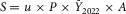
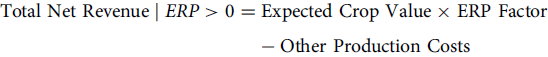 \begin{align}{{\rm Total\ Net\ Revenue} \mid ERP \gt 0} &= {\rm Expected\ Crop\ Value} \times {\rm ERP\ Factor}\\
&\quad - {\rm Other\ Production\ Costs}\end{align}
\begin{align}{{\rm Total\ Net\ Revenue} \mid ERP \gt 0} &= {\rm Expected\ Crop\ Value} \times {\rm ERP\ Factor}\\
&\quad - {\rm Other\ Production\ Costs}\end{align}
Equation 4 implies that given a non-zero ERP payment, total net revenue is always maximized at the 80 and 85% coverage levels because these two coverage levels have the highest (and identical) ERP Factors (Table 1), and Expected Crop Value and Other Production Costs are the same regardless of coverage level choice. In areas where the likelihood of receiving an ERP payment is high, this relationship may influence producer choices. Equation 4 does not imply, however, that producers should always choose 80 and 85% coverage levels. This would imply (1) that the producer is certain ex ante that future causes of loss will be in the set of ERP-eligible losses and (2) that an ERP payment is triggered simultaneously.
Consider the same under WHIPP. As mentioned, WHIPP incorporated only the gross crop insurance indemnity in the payment calculation. Modifying equation 4, total net revenue given WHIPP payments was then
 \begin{align}\eqalign{ {\rm{Total}}\;{\rm{Net}}\;{\rm{Revenue}}\mid {\rm{WHIPP}}\gt 0 &= {\rm{Expected}}\;{\rm{Crop}}\;{\rm{Value}} \times {\rm{WHIPP}}\;{\rm{Factor}}\\
&\quad - {\rm{Crop}}\;{\rm{Insurance}}\;{\rm{Premium}}\\
&\quad - {\rm{Other}}\;{\rm{Production}}\;{\rm{Costs}}}\end{align}
\begin{align}\eqalign{ {\rm{Total}}\;{\rm{Net}}\;{\rm{Revenue}}\mid {\rm{WHIPP}}\gt 0 &= {\rm{Expected}}\;{\rm{Crop}}\;{\rm{Value}} \times {\rm{WHIPP}}\;{\rm{Factor}}\\
&\quad - {\rm{Crop}}\;{\rm{Insurance}}\;{\rm{Premium}}\\
&\quad - {\rm{Other}}\;{\rm{Production}}\;{\rm{Costs}}}\end{align}
WHIPP Factors were identical to ERP Factors at the 75% coverage level and above. Therefore, given a non-zero WHIPP payment, an 80% coverage level is always preferred to an 85% because the premium at the 85% is larger. However, the preference is unclear for coverage levels below 85% coverage level. The total net revenue may be larger under the lower coverage level(s) than under the 80% coverage level depending on the relative magnitudes of the various WHIPP Factors and crop insurance premiums. The higher the coverage level, the higher the WHIPP Factor and the higher the crop insurance premium. Given the differences between ERP and WHIPP, they will have different effects on producers’ crop insurance choices.
4. Data and Methods
We conduct stochastic simulations of future market and crop yield outcomes for many representative farm operations and assume that they employ a modified expected utility approach to optimize over available coverage levels for both a baseline (no ERP) scenario and for an alternative scenario in which ERP is provided. These simulations are complex and are based on numerous data sources as described in the following subsections.
4.1. Historical Yields and Prices
For each representative farm we simulate, we require a yield history which will be used to characterize the joint distribution of crop yields, ERP payments, and crop price realizations. For the yields, we use the National Agricultural Statistics Service (NASS) county yield data as a starting point and use a similar methodology as Goodwin (Reference Goodwin2009) to construct individual representative producer yields for determining production history for each state-county-crop-type-practice (SCCTP) combination. Goodwin (Reference Goodwin2009) assumes that crop yields follow a linear trend and the deviations from trend are proportional to the trends. Specifically, we regress NASS county yields on a time trend and recover the predicted values, Ⓨ
t
, and associated residuals, ε
t
for year t. Then, we use RMA’s 2022 reference yield ${\bar Y}$
2022 for the relevant SCCTP combination to recenter the yields.Footnote
2
${\bar Y}$
2022 for the relevant SCCTP combination to recenter the yields.Footnote
2
It is widely accepted that farm-level yields present more variability than county-level yields (Claassen and Just, Reference Claassen and Just2011; Cooper et al., Reference Cooper2012; Gerlt et al., Reference Gerlt, Thompson and Miller2014; Goodwin, Reference Goodwin2009; Maisashvili et al., Reference Maisashvili, Bryant, Kpnakep and Raulston2019; Schnitkey et al., Reference Schnitkey, Sherrick and Irwin2002; Ubilava et al., Reference Ubilava, Barnett, Coble and Harri2011). Therefore, when generating a random historical representative producer’s yield, we follow Goodwin (Reference Goodwin2009) by adding an additional, zero-mean, normally distributed shock to the recentered county yields. We specify a standard deviation for this additional shock equal to 75% of that of the residuals recovered from detrending county yields (0.75σ ε ). The complete process for generating a random representative historical realized yield (Y t ) for time t is then
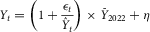 $$ Y_t = \left (1 + {\epsilon _t \over \hat{Y}_t}\right ) \times \bar{Y}_{2022} + \eta $$
 $$ \eta _t \sim N(0, 0.75 \sigma _\epsilon ) $$
For each SCCTP combination, two types of historical price series were constructed in accordance with the current Commodity Exchange Price Provisions guidelines (USDA Risk Management Agency, 2022b). Projected price (P) values were obtained as the average daily settlement price from the harvest futures contract during the projected price discovery period. Harvest price (H) values were obtained as the average daily settlement price from the harvest futures contract during the harvest price discovery period. The relevant underlying historical futures prices were purchased from CME Group. For recent years, pre-calculated P and H values were collected directly from RMA’s Actuarial Data Master (USDA Risk Management Agency, 2022a).
4.2. Starting Wealth
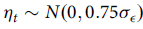
Starting wealth is an important determinant of the magnitude of ending wealth values, and consequently, the extent of curvature of the utility function in the neighborhood is relevant for evaluating simulation outcomes. Given that data are unavailable for a producer’s starting wealth, we follow Maisashvili et al. (Reference Maisashvili, Bryant and Jones2020) in obtaining estimates of starting wealth using USDA’s Agricultural Resource Management Survey Farm Financial and Crop Practices data (USDA Agricultural Resource Management Survey, 2021). Based on reported income statements and balance sheets for years 2015 through 2018, and using farm equity values as a proxy for initial wealth, they found that the value of farm equity generally was between 3.8 to 5.2 times higher than expected crop value (the product of the county reference yield, the insured price, and number of acres, A). We follow this same approach and draw a random wealth parameter for each representative farmer for a given SCCTP combination using a uniform distribution. That is, starting wealth S is given as
 $$ S= u \times P\times \bar{Y}_{2022} \times A$$
where u is a stochastic wealth parameter that is uniformly distributed over the interval [3.8,5.2].
4.3. Production Costs
Individual production costs are nearly impossible to obtain from publicly available data. Some studies have simply excluded the cost data from their analysis (Maisashvili et al., Reference Maisashvili, Bryant and Jones2020; Paulson et al., Reference Paulson, Schnitkey and Kelly2016; Ubilava et al., Reference Ubilava, Barnett, Coble and Harri2011). Goodwin (Reference Goodwin2009) argues that production costs are important factors influencing production decisions.
We collected, where available, state-level crop production costs published by the respective state extension services. If production cost data were unavailable from an extension service for a given state, we consulted USDA’s Economic Research Service commodity cost and return aggregated data for an approximation (USDA Economic Research Service, 2021).
We acknowledge that production costs are highly likely to substantially vary across individual producers and using state-level, and when necessary region-level, data can substantially deviate from the true fixed and variable expenses at the individual level. What is more, these budgets are usually prepared for a “representative” producer using recommended production practices and, as discussed by Goodwin (Reference Goodwin2009), crop budget and production costs are difficult to measure considering they are subject to individual judgment on the part of the specialist constructing the measures. However, considering that the individual cost of production data is unavailable, using state-level extension service data is a reasonable approach. We acknowledge that many individual producers have cost advantages and use varying production practices. We therefore follow Goodwin (Reference Goodwin2009) in assuming that costs are 60% of the levels implied by enterprise budgets.
We calculate crop insurance premiums using RMA’s official 2022 Actuarial Data Master (USDA Risk Management Agency, 2022a) and in accordance with the M-13 handbook (USDA Risk Management Agency, 2022c) for each SCCTP.Footnote
3
By construction of the historical yield series (as described in subsection 4.1), a representative producer’s approved yield ${\bar Y}$
used in premium calculations will be equal to the county reference yield
${\bar Y}$
used in premium calculations will be equal to the county reference yield ${\bar Y}$
2022.
${\bar Y}$
2022.
Because this research aims to explain potential changes in coverage level choices, for tractability, hypothetical corn, and soybean farms are assumed to buy revenue protection (RP). That is, we do not analyze the choice of policy type. In 2021, more than 95% of insured corn and soybean acres were insured with RP on an individual farm basis (USDA Risk Management Agency, 2021b).
4.4. ERP Related Losses
To conduct the analysis, we rely on the publicly available Cause of Loss (COL) database, which is maintained by RMA (USDA Risk Management Agency, 2021a). We collected the COL annual data from 1991 to 2021, which contains 932,084 and 808,963 total entries over 1,881 and 1,737 counties for corn and soybeans, respectively. In addition, the COL data are disaggregated by type of cause, which is determined by a claims adjuster. In total, we observe up to 50 reported causes. From the list of reported causes from the COL database, the following causes could potentially qualify for the ERP payments: cyclone, excess moisture, drought, freeze, fire, flood, hurricane/tropical depression, storm surge, tidal wave/tsunami, tornado, and volcanic eruption.Footnote 4 Figure 1 presents the distribution of indemnities by cause of loss for corn and soybeans during the 1991-2021 period. For brevity, we use a similar representation as described by Perry et al. (Reference Perry, Yu and Tack2020).

Figure 1. Crop insurance indemnity payment shares by cause of loss, 1991–2021.
For both crops, the three largest causes of indemnity payments are drought, excess moisture, and decline in price. In the case of corn, drought, excess moisture and decline in price accounted for about 38, 30 and 8.5% of payments, respectively. For soybeans, drought, excess moisture, and decline in price accounted for 33, 37, and 7.5% of payments, respectively. Considering that in a given county not all drought categories qualify for ERP, and given that the COL data do not provide further details when the specific cause is cited as drought, we queried data from the National Drought Mitigation Center at the University of Nebraska-Lincoln (2022) to categorize the COL drought data as ERP-eligible only if it was categorized as D2 for eight consecutive weeks or D3 or higher at any time during the calendar year. Specifically, the drought data identify general areas of drought and labels them by intensity, with D0 being the least intense level and D4 the most intense. The source also allows users to filter specific drought levels by consecutive weeks or by specific time spans. By merging the drought monitor data with the COL data, Figure 2 shows combined historical corn and soybean drought-related indemnities among the five drought levels (D0 through D4) in those periods when the COL was reported as drought. The figure shows that over 60% of historical corn and soybean drought-related indemnities are at the level of D2 or above.
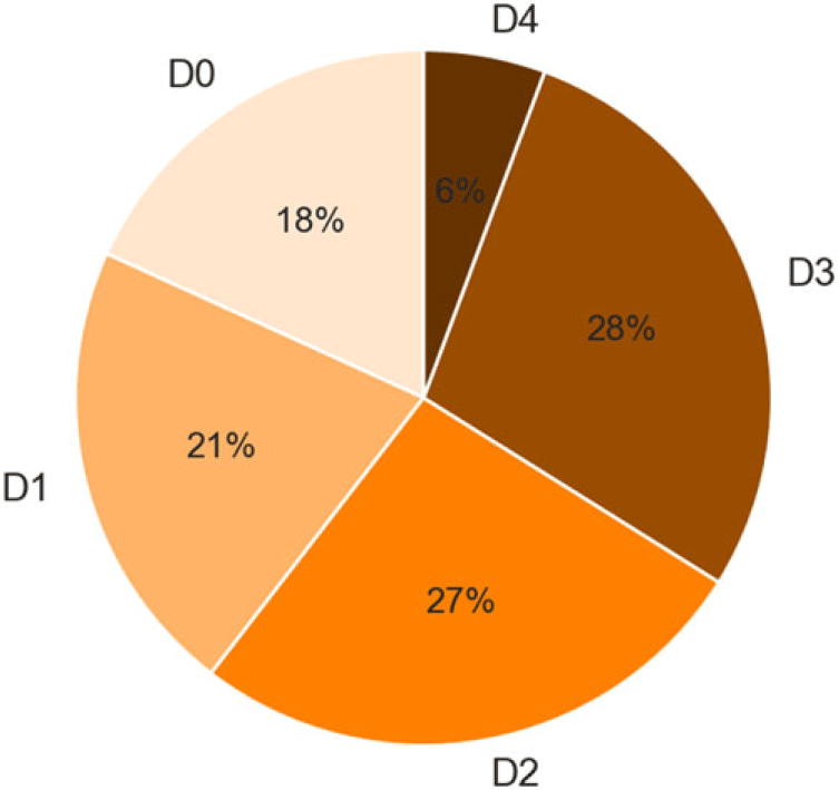
Figure 2. Drought-related combined historical corn and soybean crop insurance indemnity payment shares by drought intensity level.
For each SCCTP combination, we calculate, for 1991 through 2021, the share of the indemnified acres that could qualify for ERP payments compared to the total insured acres by creating a new variable, ranging in value between 0 and 1 for each SCCTP in given year (hereafter x q ).Footnote 5 In the simulations, this x q is employed as a directly drawn stochastic variable, as described in the following subsection.
4.5. Simulation and Dependence of Random Variables
We assume that producers optimize over probabilistic forecasts of harvest time market outcomes, which we characterize using stochastic simulation. In each simulation, we draw stochastic values for the natural log changes of harvest price with respect to observed projected prices, x p . We thus use the relation
 $$ \ln \left ( {H \over P} \right ) = x_p $$
to recover a stochastic value for the harvest time price H given the observed (at planting time) value for the known projected price P and a random draw for x p .
For crop yields, we stochastically draw x y , the natural logarithm of the realized yield relative to the producer’s approved yield. We therefore recover simulated realized yields Y using the relation
 $$ \ln \left ( {Y \over \bar{Y}} \right ) = x_y $$
given the known value ${\bar Y}$
of the approved yield and a stochastic draw for x
y
.Footnote
6
We constrain random yield draws at 0 and 150% of the RMA’s reported reference yield for relevant SCCTP combinations, similar to the approach in Goodwin (Reference Goodwin2009).
${\bar Y}$
of the approved yield and a stochastic draw for x
y
.Footnote
6
We constrain random yield draws at 0 and 150% of the RMA’s reported reference yield for relevant SCCTP combinations, similar to the approach in Goodwin (Reference Goodwin2009).
We use a multivariate kernel density estimation (MVKDE) approach to generate stochastic draws for x q , x p , and x y . This approach accommodates both arbitrary marginal densities and arbitrary non-linear relationships among variables. The multivariate kernel density estimate is
 $$ \hat{f}({\bf{{x}}}|{{\bf{B}}}, {\bf{\breve{{X}}}}) = {1 \over M} \sum _{m=1}^M \vert {{\bf{B}}} \vert ^{-1/2} \kappa \left ( {{\bf{B}}}^{-1/2} \left ( {{\bf{x}}} - \bf{\breve{{X}}}_m \right ) \right ) $$
where ${{\bf{x}}}$
is a vector of values associated with the three random variables,
${{\bf{x}}}$
is a vector of values associated with the three random variables, ${{\bf{B}}}$
is a 3 × 3 symmetric, positive definite bandwidth matrix,
${{\bf{B}}}$
is a 3 × 3 symmetric, positive definite bandwidth matrix, $\bf{\breve{{X}}}$
is a sample of M historical observations for the three variables, κ is a symmetric multivariate density function whose mean is a vector of three zeros, and
$\bf{\breve{{X}}}$
is a sample of M historical observations for the three variables, κ is a symmetric multivariate density function whose mean is a vector of three zeros, and ${\bf{\breve{{X}}}}_m$
reflects the m
th observation in the data sample.
${\bf{\breve{{X}}}}_m$
reflects the m
th observation in the data sample.
We use a Gaussian PDF for κ, and the kernel density then becomes
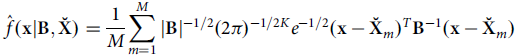 $$ \hat{f}({{\bf{x}}}|{{\bf{B}}}, {\bf{\breve{{X}}}}) = {1 \over M} \sum _{m=1}^M \vert {{\bf{B}}} \vert ^{-1/2} (2\pi )^{-1/2K} e^{-1/2} ({\bf{x}} - {\bf{\breve{{X}}}}_m)^T {{\bf{B}}}^{-1} ({{\bf{x}}} - {\bf{\breve{{X}}}}_m) $$
where ${{\bf{B}}}$
in this context would be the covariance matrix for a multivariate (non-standard) normal distribution. Consistent with Gerlt et al. (Reference Gerlt, Thompson and Miller2014), we apply Silverman’s rule for the bandwidth selection (Silverman, Reference Silverman1986), where the off-diagonal elements of
${{\bf{B}}}$
in this context would be the covariance matrix for a multivariate (non-standard) normal distribution. Consistent with Gerlt et al. (Reference Gerlt, Thompson and Miller2014), we apply Silverman’s rule for the bandwidth selection (Silverman, Reference Silverman1986), where the off-diagonal elements of ${{\bf{B}}}$
are zero and the k
th diagonal element is, for this three variable application, given by
${{\bf{B}}}$
are zero and the k
th diagonal element is, for this three variable application, given by
 $$ \sqrt{{{\bf{B}}}_{kk}} = \sigma _k \left ({{4M \over 5}}\right )^{-1/ 7} $$
where σ k is the sample standard deviation for the k th variable.Footnote 7 Alternatively, we could have employed copula-based methods, which provide a means to model dependency among random variables with mixed marginal distributions. Copula-based models have been used in various applications (Fei et al., Reference Fei, Vedenov, Stevens and Anderson2021; Nadolnyak and Vedenov, Reference Nadolnyak and Vedenov2013; Power et al., Reference Power, Vedenov, Anderson and Klose2013; Woodard et al., Reference Woodard, Paulson, Vedenov and Power2011), including crop insurance (Goodwin and Hungerford, Reference Goodwin and Hungerford2015; Ramsey et al., Reference Ramsey, Goodwin and Ghosh2019). We chose to use the MVKDE approach, however, due to its ability to represent any arbitrary multivariate dependence structure.
4.6. Indemnity Calculations
Given stochastic realizations for the harvest price, H, and a representative producer’s individual yield, Y, we follow RMA’s procedures (USDA Risk Management Agency 2022d) for crop insurance indemnity (I) calculations:
 $$ I_C = max\{0, [(C \times \bar{Y} \times max\{P, H\}) - Y\times H]\} \times A$$
where C is a crop insurance coverage level for a given scenario, between 50 and 85% in 5% increments, and A is the insured acreage.
4.7. Ending Wealth
For the baseline scenario, a producer’s ending wealth E for trial i for a given coverage level C is calculated as follows:
 $$ E_{C, i} = S+ (H_i \times Y_i + I_{C, i} - R_C - V) \times A$$
where S is producer’s starting net worth (as described in subsection 4.2), H i is the stochastic harvest time price, Y i is the stochastic realization of the crop yield; I C, i is crop insurance indemnity (a function of Y, H, and C), R C is the producer premium for coverage level C, V is deterministic variable expenses other than insurance premiums (as described in subsection 4.3), and A is insured acreage. Here, we abstract from basis considerations, so that market revenue is simply H × Y.
For counterfactual scenarios that include an ERP payment, ending net worth is
 $$ E_{C, i} = S+ (H_i \times Y_i + I_{C, i} - R_C - V+ x_{q, i} \times W) \times A$$
where W is a per-acre ERP payment per equation 1.
4.8. Modified Expected Utility Framework
To analyze the impacts of the ERP program on coverage level decisions, we assume that producers’ decisions are dependent on the distribution of ending net worth (E). An expected utility approach for ranking risky alternatives has been used widely in the crop insurance literature (Babcock, Reference Babcock2015; Coble et al., Reference Coble, Knight, Pope and Williams1996; Du et al., Reference Du, Ifft, Lu and Zilberman2015, Reference Du, Feng and Hennessy2017; Du et al., Reference Du, Feng and Hennessy2017; Goodwin, Reference Goodwin1993; Goodwin, Reference Goodwin2009; Hardaker, Reference Hardaker2004; Hennessy, Reference Hennessy1998; Mahul, Reference Mahul1999; Maisashvili et al., Reference Maisashvili, Bryant and Richardson2016; Maisashvili et al., Reference Maisashvili, Bryant and Jones2020; Paulson et al., Reference Paulson, Schnitkey and Kelly2016; Richardson et al., Reference Richardson, Herbst, Outlaw and Gill2007; Ubilava et al., Reference Ubilava, Barnett, Coble and Harri2011).
Preliminarily, suppose that producers exhibit constant relative risk aversion (CRRA) (following Goodwin, Reference Goodwin2009; Paulson et al., Reference Paulson, Schnitkey and Kelly2016; Ubilava et al., Reference Ubilava, Barnett, Coble and Harri2011). There is mounting evidence directly supporting CRRA under the basic expected utility framework (Brunnermeier and Nagel, Reference Brunnermeier and Nagel2008; Chiappori and Paiella, Reference Chiappori and Paiella2011; Sahm, Reference Sahm2012). CRRA implies an isoelastic utility function:
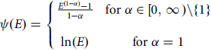 \begin{align}\psi (E) = \left\{ {\matrix{
{{{{E^{(1 - \alpha )}} - 1} \over {1 - \alpha }}} & {{\rm{for}}\;\alpha \in [0,\infty )\backslash \{ 1\} } \cr
{\ln (E)} & {{\rm{for}}\;\alpha = 1} \cr
} } \right.\end{align}
\begin{align}\psi (E) = \left\{ {\matrix{
{{{{E^{(1 - \alpha )}} - 1} \over {1 - \alpha }}} & {{\rm{for}}\;\alpha \in [0,\infty )\backslash \{ 1\} } \cr
{\ln (E)} & {{\rm{for}}\;\alpha = 1} \cr
} } \right.\end{align}
where α is a producer’s coefficient of CRRA.
Then, a producer’s certainty equivalent income across N simulated trials for a given coverage level C is:
 $$ \psi _\alpha ^{-1} \left ( {1 \over N} \sum _{i=1}^N \psi _\alpha (E_{C, i}) \right ) $$
where ψ α −1 is the inverse utility function conditioned on the CRRA coefficient α.
However, our preliminary investigation revealed that a basic expected utility approach cannot reasonably reproduce producers’ observed crop insurance choices. In many instances, under the modeling approach laid out above, no non-negative coefficient of CRRA will result in lower coverage levels, such as 75%, having the highest certainty equivalent, even though we observe a non-trivial proportion of producers choosing 75% coverage. Therefore, simple producer heterogeneity cannot salvage the basic expected utility framework under our modeling approach. Many previous studies have observed this shortcoming of the basic expected utility approach, as applied to producers’ crop insurance choices (Babcock and Hart, Reference Babcock and Hart2005; Babcock, Reference Babcock2015; Du et al., Reference Du, Hennessy and Feng2013; Du et al., Reference Du, Feng and Hennessy2017; Luckstead and Devadoss, Reference Luckstead and Devadoss2019; Michaud, Reference Michaud2021). This motivates us to pursue either an alternative theory of decision-making under risk or modifications to the expected utility approach.
We do, however, wish to acknowledge that producers are likely heterogeneous. The SOB data show that for a given SCCTP combination, even though there may be a dominant coverage level which producers mostly purchase, a non-trivial portion of farmers opt to purchase other coverage levels. As an example, the 2021 RMA Summary of Business (SOB) data show that in Boone County, Iowa, a large portion of corn and soybean acres were insured under 80 and 75% coverage levels, even though the 85% coverage level is the most popular (Figure 3). Likewise, in many counties where 70 and 75% coverage levels are the most popular choices, a non-trivial portion of producers buy 80 and 85% coverage. We require our approach to accommodate this feature of the observed data.
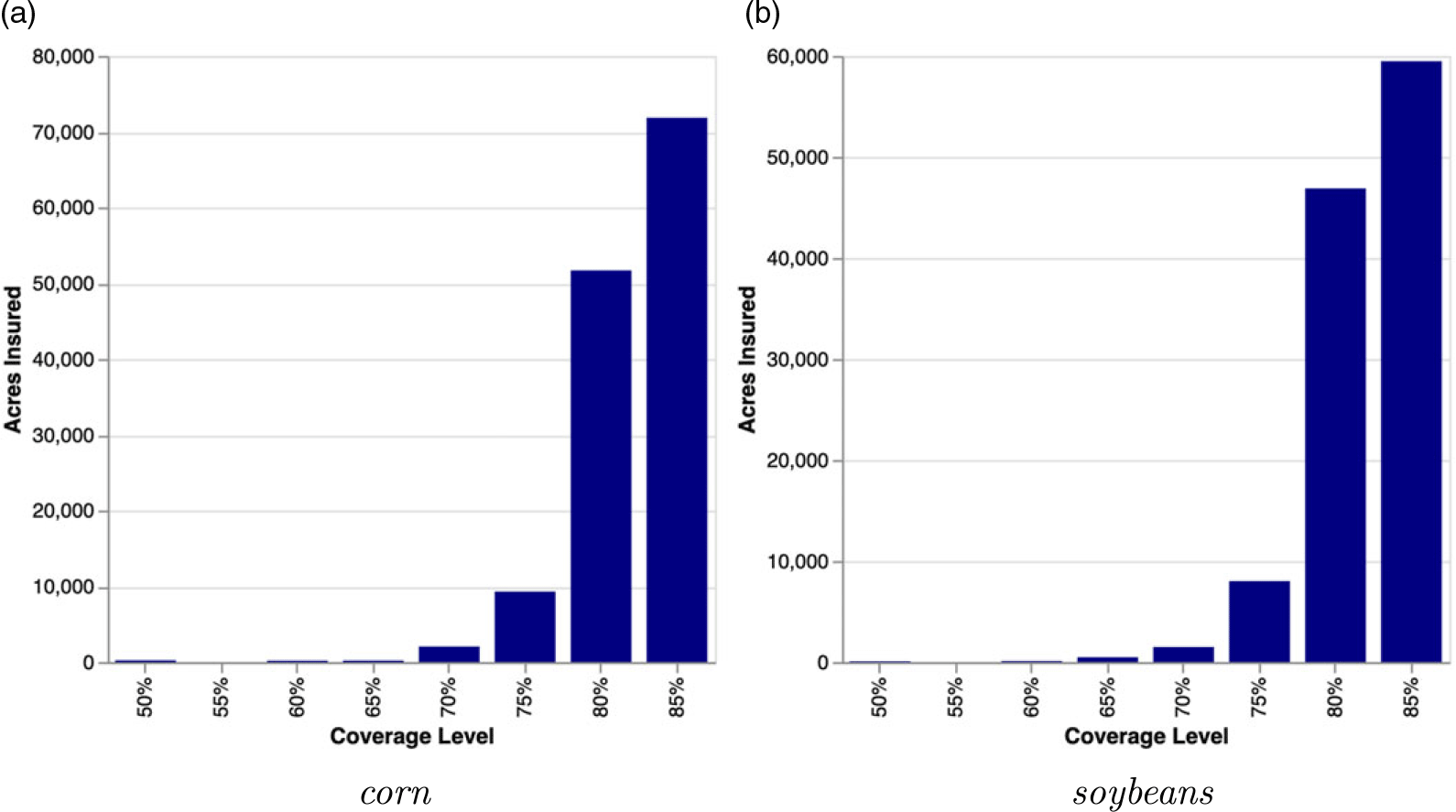
Figure 3. Actual coverage level choices observed in 2021 for corn and soybean producers in Boone County, Iowa.
Du et al., (Reference Du, Feng and Hennessy2017) suggest that farmer preferences for crop insurance coverage might be captured by cumulative prospect theory initially proposed by Tversky and Kahneman (Reference Tversky and Kahneman1992). Babcock (Reference Babcock2015) found that cumulative prospect theory does explain coverage level choices that are consistent with the observed SOB choices only if crop insurance is a lottery considered in isolation. Babcock finds, however, that if a producer’s overall portfolio (market revenue, in addition to crop insurance premiums and indemnities) is the lottery under consideration, then the optimal choices suggested by cumulative prospect theory are not consistent with observed choices. Optimal choices for producers’ overall portfolios are exactly the problem we consider here, and we therefore do not apply cumulative prospect theory.
If farmers do not make choices according to straight expected utility or cumulative prospect theory, one potential explanation could be that they select the coverage level that is simply “good enough.” This may be due to one or more of several possible reasons: cognitive constraints (Simon, Reference Simon1955, Reference Simon1956; Tversky and Kahneman Reference Tversky2013), non-negligible computational burden (Newell and Simon, Reference Newell and Simon1972; Simon, Reference Simon1997; Van Rooij Reference Van Rooij2008; Lieder and Griffiths, Reference Lieder and Griffiths2020), or information acquisition costs (Bogacz et al., Reference Bogacz2006; Gabaix et al., Reference Gabaix, Laibson, Moloche and Weinberg2006; Sims, Reference Sims2003; Sims, Reference Sims2006). Analysis whereby agents select alternatives that are “good enough” has been conducted in the economic literature as well (see Dickhaut et al., Reference Dickhaut, Rustichini and Smith2009; Gabaix et al., Reference Gabaix, Laibson, Moloche and Weinberg2006; Sims, Reference Sims2003; Verrecchia, Reference Verrecchia1982; Vulkan, Reference Vulkan2000; Woodford, Reference Woodford2014).
The challenge in implementing such an approach is defining what “good enough” is, and how an agent chooses among a set of multiple options that are good enough. We adopt a simple and intuitive approach. First, we assume a fixed reasonable value for the relative risk aversion parameter. Then, we specify a neighborhood of certainty equivalent values that are approximately maximal (including the one exactly maximal certainty equivalent). We then define the coverage level choices corresponding to the certainty equivalents in this neighborhood as the satisficing set. We then assume that producers choose from this set at random.
Many different values for the relative risk aversion coefficient have been employed in the literature. For example, Anderson and Dillon (Reference Anderson and Dillon1992) propose the values between 0 and 4, where 0 implies a risk-neutral individual and 4 corresponds to an extremely risk-averse agent. Hennessy (Reference Hennessy1998) used values in the range of 4.1 and 9.7. Goodwin (Reference Goodwin2009) employed values from 0 to 15. Paulson et al. (Reference Paulson, Schnitkey and Kelly2016) selected coefficients between 0 and 12; McSweeny and Kramer (Reference McSweeny and Kramer1986) selected values between 2.5 and 11.5. Michaud (Reference Michaud2021) used a coefficient of 0.12 to represent a mildly risk-averse individual. Here, we employ a relative risk aversion coefficient of 2.5 to represent a moderately risk-averse decision maker, as suggested by some of the aforementioned literature, in addition to other studies (Lien and Hardaker, Reference Lien and Hardaker2001; Lusk and Coble, Reference Lusk and Coble2005; Maisashvili et al., Reference Maisashvili, Bryant and Jones2020; Ubilava et al., Reference Ubilava, Barnett, Coble and Harri2011).
For each SCCTP combination, the specific steps in our approach are as follows.
-
Step 1: We generate 20 representative producers, each with a random starting wealth (per subsection 4.2).
-
Step 2: For each representative producer, we simulate ending wealth and calculate certainty equivalents for each of the eight available coverage levels using equation 17 with α = 2.5.
-
Step 3: For each representative producer, we randomly draw a satisficing threshold parameter between 0 and 2% from a uniform distribution. We then determine the set of coverage level choices with certainty equivalent values that are less than the maximum certainty equivalent by no more than this percentage. This is the satisficing set.
-
Step 4 (baseline scenario): In the context of no ERP, for each coverage level in the satisficing set, we assume that producers select at random, with probabilities equal to the relative proportions of acres covered at that level in the SOB data for the relevant SCCTP.
-
Step 4 (ERP scenario): For the counterfactual scenario, we assume that a representative producer changes to a new coverage level if that coverage level both newly enters (vis-à-vis the baseline scenario) the satisficing set and has a certainty equivalent that is greater than their previous choice.
This last rule regarding changing coverage level choice under the ERP scenario is clearly not the only criterion that could be specified. Indeed, one might argue that this rule violates the spirit of the satisficing set. We also considered an alternative rule whereby producers changed coverage level only if their original choice fell out of the satisficing set. This resulted in very nearly zero changes in coverage level choice across all SCCTPs we consider. Even though there is little point in presenting those results in detail, we acknowledge that essentially zero changes in crop insurance choices may indeed be reasonably interpreted as the correct answer. We present results below that reflect the change rule presented above and interpret the resulting projected changes as the maximum extent of coverage level changes that might reasonably be expected to result from permanent authorization of the ERP program.
4.9. Model Validation
To validate the model, we ran the baseline scenario (no ERP) and compared it with observed choices in the SOB data. In total, we analyzed 67 million acres of dryland corn and 63 million acres of dryland soybeans. Results for 3,622 individual SCCTP combinations were aggregated and are summarized in Figure 4, which shows coverage level choices, measured in acres.

Figure 4. Validation results (simulated vs. summary of business) for the baseline scenario.
The two most popular coverage levels for both crops are 75 and 80%, whereas using a direct expected utility maximization framework would have over-selected an 85% coverage level in a substantial portion of counties for the reasons described above.
The validation result shows that the model slightly under-selects 85% coverage levels and moderately over-selects the 80% coverage levels. The simulation results showed that combined insured acres for corn and soybeans under the 75, 80, and 85% coverage levels were 58 and 53 million acres, when compared to the SOB data of 56 and 54 million acres, respectively.
5. Results
For each of the 3,622 SCCTP combinations, we conducted 500 trials of the simulation described in the previous section for both the baseline and alternative ERP scenarios. The results are decomposed into several regions, with the states included in each regional division being presented in Table 2. Before discussing the main results, we briefly describe Spearman’s rank correlation statistics that resulted from the MVKDE procedure among the three random variables, x p , x y , and x q . The average regional values, along with interquartile ranges, for corn and soybeans are presented in Tables A1 and A2 in the appendix. We find strong negative dependencies between x p and x y in major corn and soybean production areas, including the Corn Belt and Central Plains, under both crops. Although negative, on average, the regional rank correlation between x p and x y is relatively weak in the other areas. The dependence between x q and x y is negative, and quite strong, across all regions for both crops. The higher the share of ERP-related losses with respect to the insured acres, the lower the realized yield with respect to the approved yield. The dependencies are stronger in the Corn Belt, Central Plains, and Lake States regions. With regard to the rank correlation between x p and x q , we observe, on average, a positive relationship across all regions. The higher the share of ERP-related losses, the higher the harvest price with respect to observed projected price. The average values are larger in the Corn Belt, Central Plains, and Northern Plains regions than in other areas. The dependencies are weak in the Lake States, South East, and Southern Plains and Other regions.
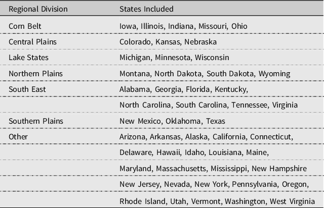
Table 2. Regional division and corresponding states
Aggregated changes in total crop insurance premiums collected (sum of the producer premiums and subsidies), expected ERP payments, and expected per-acre payments from the program are presented in Table 3.Footnote 8 As discussed in the methodology section, because of the decision rule applied to determine if a representative producer changes coverage levels, we interpret the results presented here as the maximum extent of crop insurance choice changes that might reasonably be expected due to a permanent authorization of the ERP program.Footnote 9
Table 3. Change in total premiums, expected per-acre and total ERP payments

5.1. Coverage Level Changes
The nature of changes in farmer choices for corn and soybeans for the 8 coverage levels are presented in Figure 5. The results for both crops are similar. For corn producers, aggregate insured acres under the 85% coverage level are projected to decline from 13.3 million to 13.2 million. Aggregate insured acres under the 80% coverage level are projected to increase from 22 million to 22.5 million. Aggregate acres insured under the 75 and 70% levels are projected to decline from 30.6 million to 30.3 million. Aggregate acres insured under the coverage levels below 70% are projected to have negligible changes.

Figure 5. Simulation results of baseline and counterfactual scenarios for corn and soybean.
For soybeans, the magnitude of changes in insured acres is slightly larger than that of corn. Simulation results indicate that aggregate insured acres under the 85% coverage level are expected to decrease from 11.2 million to 10.8 million, while aggregate acres insured under the 80% level are projected to increase from 20.5 million to 21.5 million. Aggregate acres insured under the 75 and 70% levels are projected to decline from 29.4 million to 28.8 million. Similar to corn, negligible changes are projected below the 70% coverage level.
Therefore, for both crops, the ERP program is unlikely to influence the optimal coverage level choices for most producers. However, a small number of producers who currently purchase the highest coverage level (85%) may be compelled to move toward the 80 and 75% coverage levels, while a small number of producers who currently opt for the 70 and 75% coverage levels may be incentivized to move towards the 80% coverage level.
There are two forces contributing to these results. First, expected ERP payments account for a small share of total farm revenue, which includes crop sales, crop insurance indemnities, and other government payments. Thus, the actual impact of ERP payments on producer decisions is likely to be modest. Second, the 75, 80 and 85% crop insurance coverage levels map to very similar ERP factors (a 95% ERP Factor for the 80 and 85% coverage levels and a 92.5% ERP Factor for the 75% coverage level), meaning that additional utility gains from the ERP program due to higher coverage levels are not large enough to entice a significant number of producers in the 70 and 75% coverage level to buy up further. Indeed, our results suggest that the free protection provided by the ERP program may make some producers currently at the (85%) coverage level comfortable in somewhat relaxing that protection.
5.2. ERP Payments and Crop Insurance Premiums
Changes in collected total insurance premiums and expected ERP payments by region and nationally are presented in Table 3. We project that permanently authorizing the ERP program would result in an increase in total premiums collected of up to $10.6 million across both crops. For perspective, collected premiums for non-irrigated corn and soybeans combined exceeded $6.6 billion in 2021 (USDA Risk Management Agency, 2021b), implying that permanently authorizing the ERP program is projected to result in a very small percentage change in collected crop insurance premiums. Combined expected ERP payments for both crops are projected to be $1.28 billion ($835 million in case of corn and $446 million for soybeans). The magnitude of projected payments is higher than they would likely have been in the previous years because of the historically high projected crop prices for year 2022 (USDA Risk Management Agency, 2022e).
The largest ERP payments for corn and soybeans would be in the Corn Belt region, where 46% of corn acres and 45% of soybeans acres are insured. What is more, excessive moisture and qualifying drought account for more than 50% of insurance indemnities when a loss is declared (Figure 1), which further increases the magnitude of total projected ERP payments when compared to the other regions. Total projected ERP payments in the region are $437 million for corn and $212 million for soybeans.
The projected decrease in total premiums collected for the Corn Belt is estimated to be $1.8 million for both crops combined. While this change is modest, it is the only region where the projected change is negative. The reason behind this is that many Corn Belt producers purchase the highest coverage level (85%), where the incentive to “buy-down” to lower coverage levels (80 and 75%) is slightly greater. In other regions, a larger portion of acres are insured under the 70 and 75% coverage levels.
The Lake States and Northern Plains regions are projected to have relatively large ERP payments for both crops annually, totaling $243 million and $128 million, respectively. However, the combined projected changes in collected total premiums are modest considering that producers mostly purchase mid-range coverage (70 and 75%) for the baseline scenario, and the ERP Factor schedule, except for a small number of producers, provides limited incentive to buy up to higher coverage levels but does discourage switching to lower coverage levels.
Similar results are found in the South East and Southern Plains regions as well. The total ERP payment in both regions for both crops combined is projected to be over $89 million, but relatively trivial changes are observed in terms of collected total premiums.
5.3. ERP Program and Expected Per-acre Payments
The distributions of county per-acre ERP payments are illustrated in Figures 6 and 7. The histograms characterize the dispersion of payments across counties for each crop, grouped by region.
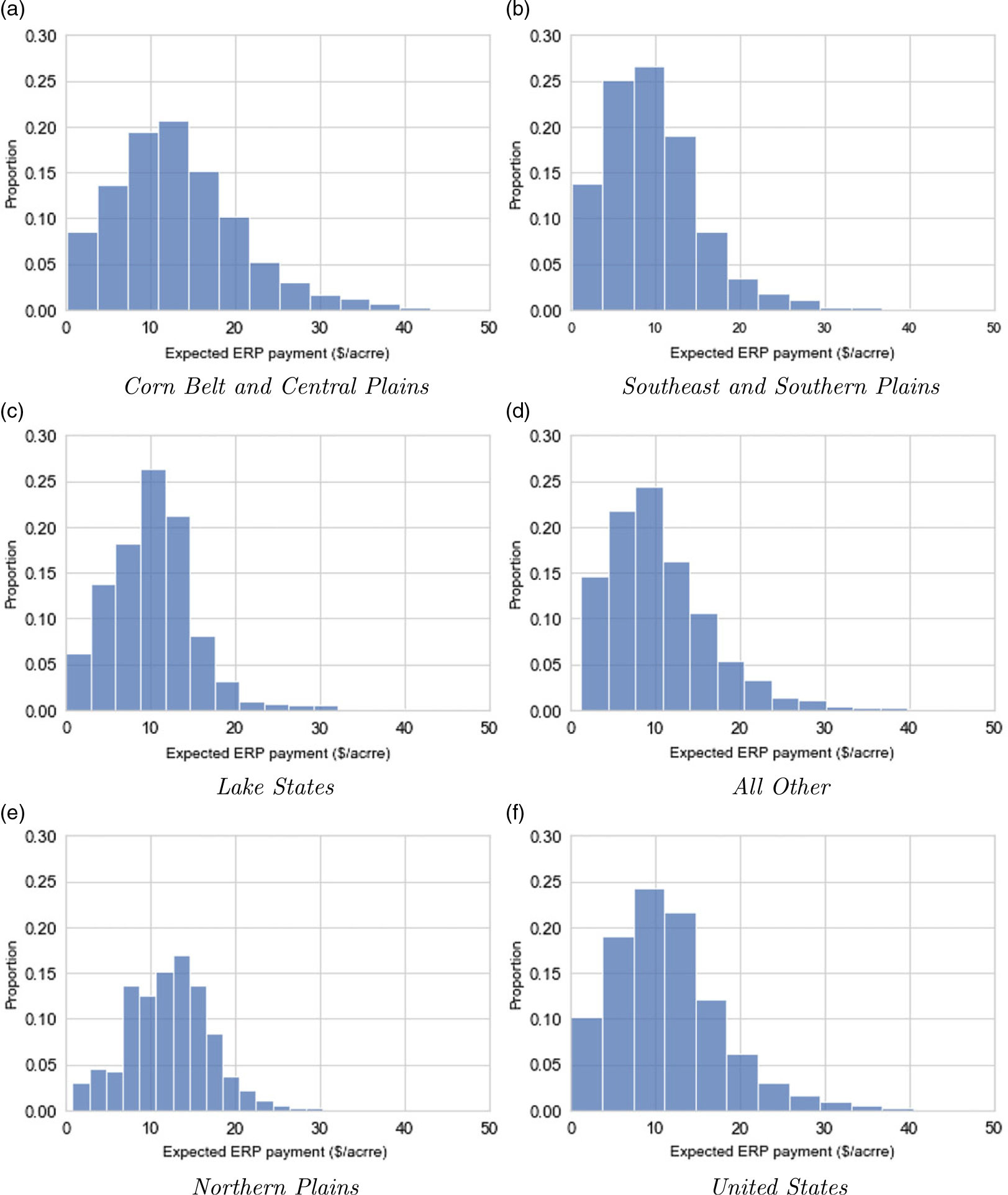
Figure 6. Distributions of county expected ERP payments for corn ($ per acre).
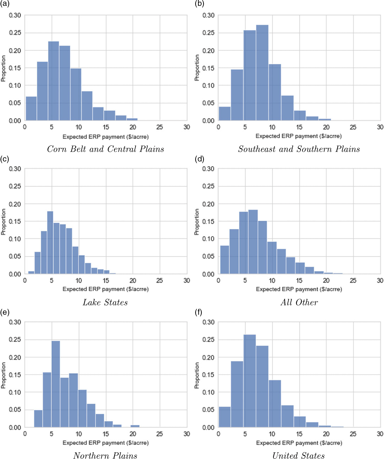
Figure 7. Distributions of county expected ERP payments for soybeans ($ per acre).
Expected per-acre payments (averages of simulated values across 500 trials) for corn and soybeans are projected to total $11.4 and $7.3, respectively, for the United States. The distributions of the ERP simulated payments have a strong positive skew, where the median value for the majority of the SCCTP combinations is $0. That is, the 50th percentile of ERP payments has $0 per-acre payments for the majority of SCCTP combinations. Although the national expected payment for corn is around $11.4 per acre, the average value is larger in the Corn Belt region, at around $15.3 per acre. The same is true for soybeans in the Corn Belt and Northern Plains regions, where expected per-acre payments are projected to be $7.5 and $7.8 per acre, respectively, compared to the average national value of $7.3 per acre. This is mainly because expected crop values, at least in the case of corn, which is one of the main components of the ERP calculation formula, are relatively large in the Corn Belt region because of higher expected yields when compared to the other regions (see equation 1).
6. Implications and Limitations
We analyzed the interaction of the ERP program with crop insurance coverage level decisions. We simulated prices, representative producer yields, and historical shares of the program-related losses for non-irrigated corn and soybean farmers. Although nationwide average ERP payments per acre could be as high as $11.4 and $7.3 for corn and soybeans, respectively, we find that the program payments will have, at most, a modest effect on optimal crop insurance coverage level decisions. A small number of producers currently purchasing the highest coverage could be compelled to move toward mid-range coverage levels. Expected ERP payments, on average, are relatively small when compared to expected crop revenues, other government payments, and crop insurance indemnities. In high-production areas (e.g. the Corn Belt and Central Plains), the program yields the greatest utility when the coverage level is either 75 or 80%, but most of the corn and soybean acres are insured under these levels already. Because ERP Factors increase as a producer’s coverage level increases, the introduction of ERP into their coverage level optimization problem implies competing additional incentives: an incentive to decrease their coverage level because of new free loss protection from the government, but also an incentive to increase their coverage level to increase ERP payments in the event of a covered loss. As a result, the actual effect of ERP payments on producer crop insurance coverage level decisions will be modest. Specifically, for both crops combined, the maximum change in total premiums collected that might reasonably be expected is approximately $10.6 million.
Climate-related natural disasters have long plagued production agriculture around the world, but they are becoming more frequent and costly (World Meteorological Organization, 2021). It should come as no surprise, then, that the U.S. Congress has funded WHIP, WHIPP, and ERP for five consecutive years in response to a number of natural disasters. While these programs have helped producers respond to disasters, the aid is uncertain and is delivered long after the natural disaster has come and gone. Beyond the natural disasters, fluctuations in the availability and cost of agricultural inputs due to ongoing supply chain disruptions and unrest in Eastern Europe have led to additional calls for assistance for agricultural producers. While this assistance could come in many forms – for example, additional income support via the next farm bill or increases to crop insurance coverage levels and premium support – some are calling for disaster programs like ERP to be permanently authorized. For policy makers, that naturally raises questions about interactions with existing programs. Given the prominence of crop insurance, most policy makers are sensitive about doing no harm. This study shows that ERP in its current form – if it were permanently authorized – would have a negligible effect on crop insurance. With that said, Congress may still opt for improvements to crop insurance in lieu of permanently authorizing disaster assistance, in part (1) producers share in the cost of crop insurance and (2) permanently authorizing disaster assistance is costly (i.e. an estimated $1.28 billion per year for corn and soybeans alone).
Our study reflects important limitations. First, the modified expected utility framework we employed arguably suggests coverage level changes under overly permissive circumstances, leading to us interpreting our results regarding coverage level changes as an upper bound on what might occur. Second, ERP includes excessive moisture as one of the main qualifying disaster events, but the program documentation provides limited details regarding the conditions that trigger an event declaration. Therefore, we assumed a direct correspondence between the ERP excess moisture determination and that reflected in RMA’s Cause of Loss data. As seen in Figure 1, excessive moisture accounts for a large share of all reported occurrences, and the fine details of which events qualify will certainly affect the results. Future research could incorporate a more nuanced representation of excessive moisture.
Data Availability Statement
Data are retrieved from public domain resources.
Author Contributions
Conceptualization, A.M., B.F., H.B.; Data Curation, A.M.; Formal Analysis, A.M., B.F., H.B.; Funding Acquisition, B.F.; Methodology, A.M. and H.B.; Software, A.M. and H.B.; Visualization, A.M., B.F., and H.B.; Writing-Original Draft, A.M.; Writing-review & editing, B.F. and H.B.
Funding statement
This research was supported in part by USDA cooperative agreement 58-0111-21-006.
Competing Interests
Aleksandre Maisashvili, Bart Fischer, and Henry Bryant declare none.


 Open access