


1. Introduction
Particulate systems involving long-range interactions are difficult to study, especially with the presence of inhomogeneity. In the field of multiphase flows, numerical simulations have been performed by many researchers (e.g. Patankar & Joseph Reference Patankar and Joseph2001; Zhang & Prosperetti Reference Zhang and Prosperetti2005; Wang et al. Reference Wang, Peng, Guo and Yu2016; Subramanian & Balachandar Reference Subramanian and Balachandar2017; Theofanous & Chang Reference Theofanous and Chang2018; Yao & Capecelatro Reference Yao and Capecelatro2018). Most, if not all, of them are limited to homogeneous systems. The assumption of statistical homogeneity is needed in many numerical calculations not only for convenience in the post-processing of the numerical results, but for the validity of the numerical methods in dealing with the long-range interactions among the particles. For instance, the use of periodic boundary conditions in numerical simulations and the treatment (O'Brien Reference O'Brien1979) of the surface integral at infinity in Stokesian dynamics (Brady & Bossis Reference Brady and Bossis1988) all require the absence of volume fraction gradient because of the long-range hydrodynamic interactions. Similar situations also exist in other fields of physics. For instance, numerical simulations of charged particles often rely on the Ewald sum (Nestler, Pippig & Pott Reference Nestler, Pippig and Pott2015; Rackers et al. Reference Rackers, Liu, Ren and Ponder2018; Yao & Capecelatro Reference Yao and Capecelatro2018) in a periodic domain and the assumption of charge neutrality to avoid divergent integrals caused by Coulomb forces among the particles. To study an inhomogeneous particulate system, one inevitably needs to consider interactions between the macroscopic length scale at which the mean fields change and the scale of mean particle separation. The long-range interactions cannot be categorized into either of the scales. This difficulty is reflected in the calculation of mean properties, where divergent integrals are often encountered. It will be useful to have a method capable of calculating averages without the difficulties of the divergent integrals.
The main objective of this work is to rigorously establish a relation between the ensemble average and the nearest particle statistics. Because of the rapid far-field decay of the nearest particle probability density function, the integral relating the ensemble average and the average conditional on the nearest particle converges absolutely; therefore it is potentially a powerful method to study long-range particle interactions without the difficulty of a divergent integral, especially in processing data from numerical simulations.
The nearest particle probability is an old concept (Hertz Reference Hertz1909; Chandrasekhar Reference Chandrasekhar1943). Its use to study effective properties in multiphase flows has also been proposed (Drew & Mandyam Reference Drew and Mandyam1997). Without a rigorously derived relation between the ensemble average and the nearest particle statistics, there are many questions regarding the legitimacy of its use. These questions include the effect of other nearby particles and the order of the asymptotes of the average quantities at the limit of a small particle volume fraction  $\theta _p$. For instance, the typical distance between particles scales as $\theta _p^{-1/3}$. For a method based on the interparticle distance, does this imply that the primary effect of the volume fraction to an average quantity, such as the drag force, is of order $\theta _p^{1/3}$? For a particle, between the typical distance to its nearest particle and the distance twice of that, often there are ten or more particles. How can one account for the effects of these particles?
These questions will be answered at the end of the next section after deriving the relation between the ensemble phase average and the nearest particle statistics and by the example in § 3. As an application of the relation, in § 3, the Stokes drag and the particle sedimentation velocity are calculated following the steps of Batchelor (Reference Batchelor1972) for a flow with a dilute particle phase, but without using the renormalization techniques. In this way the new method is compared with the renormalization method.
Although the particle sedimentation velocity is a half-century-old problem, and the theory of multiphase flows has progressed considerably beyond the work of Batchelor (Reference Batchelor1972). For instance, it is now known that the relative motion between the particle and the fluid phases results in microstructures of the particles affecting the sedimentation velocity (Ham & Homsy Reference Ham and Homsy1988; Cichocki & Sadlej Reference Cichocki and Sadlej2005; Felderhof Reference Felderhof2008). The divergent nature associated with long-range particle interactions and their treatments is still a subject of modern research (Piazza Reference Piazza2014; Rackers et al. Reference Rackers, Liu, Ren and Ponder2018). The work of Batchelor (Reference Batchelor1972) is still viewed as a significant reference point because of the physical insights, despite the simplification assumptions used. We revisit this sedimentation problem with the new relation to understand the physics contained in the quantities conditionally averaged on the nearest particle. In the process, we also learn how the new relation avoids the need for the difficult renormalizations, and how the effects of the particles other than the nearest one are included. For this purpose, before applying the relation to more complex realistic systems (Fiore, Wang & Swan Reference Fiore, Wang and Swan2018), we choose to start with the simplified system studied by Batchelor (Reference Batchelor1972), assuming a statistically homogeneous and isotropic particle distribution.
In § 4, we show that the correlation product of the nearest particle distance and the fluid force on a particle is a stress tensor containing information of particle interactions at the interparticle length scale. This stress is similar to the potential part of the virial stress in a molecular system. Its divergence is a force density important for statistically inhomogeneous flows. This application shows that the nearest particle statistics cannot only recover classical results, but can also be used to study new physics. Furthermore, the renormalization technique is limited to linear problems, while the new relation is rather general. Without the divergence difficulty, the nearest particle statistics can be used to study a large variety of long-range particle interactions, such as charged particles in plasma and colloidal systems (Allen & Tildesley Reference Allen and Tildesley2017) and gravitational effects on galaxies.
2. Ensemble phase average and nearest particle statistics
2.1. Average for the continuous phase
Let  $\mathscr {P}$ be the probability measure (Ash Reference Ash1972) defined on subsets of a collection (ensemble, or sample space) of disperse multiphase flows, and $\mathscr {F}$ be a multiphase flow in the sample space, which is often represented by a list of variables, including the fields of particle positions, shapes, velocities, boundary values, etc., that uniquely and completely describes the multiphase flow. To allow for generality while simplifying our notation, here we use the abstract concept (Ash Reference Ash1972) of probability $\mathscr {P}$. If flow $\mathscr {F}$ can be represented by a finite set of parameters ( $\lambda$), then $\mathscr {F} = \{\lambda _1, \lambda _2, \ldots , \lambda _n\}$ and $\textrm {d} \mathscr {P} = P(\lambda _1, \lambda _2, \ldots , \lambda _n) \,\textrm {d}\lambda _1 \,\textrm {d} \lambda _2 \ldots \textrm {d}\lambda _n$, with $P(\lambda _1, \lambda _2, \ldots , \lambda _n)$ being the probability density in the $n$-dimensional phase space formed by the parameters. Unfortunately, most multiphase flows cannot be described simply by a finite number of parameters because of the degrees of freedom associated with the continuous phase. The only exceptions are the Stokes and potential flows with boundary conditions specified without uncertainties.
The indicator function  $\chi _c(\boldsymbol {x}, t, \mathscr {F})$ for the continuous phase is defined such that $\chi _c(\boldsymbol {x}, t, \mathscr {F}) =1$, if at time $t$ position $\boldsymbol {x}$ is occupied by the continuous phase in flow $\mathscr {F}$, and $\chi _c(\boldsymbol {x}, t, \mathscr {F}) =0$, otherwise. The volume fraction of the continuous phase is defined as (Zhang & Prosperetti Reference Zhang and Prosperetti1994, Reference Zhang and Prosperetti1997; Zhang et al. Reference Zhang, VanderHeyden, Zou and Padial-Collins2007)
 \begin{equation} \theta_c(\boldsymbol{x}, t) = \int \chi_c(\boldsymbol{x}, t, \mathscr{F}) \,\textrm{d} \mathscr{P}. \end{equation}
For a generic continuous phase quantity  $q_c (\boldsymbol {x}, t, \mathscr {F})$ in flow $\mathscr {F}$ at position $\boldsymbol {x}$ and time $t$, its ensemble phase average is defined as
 \begin{equation} \langle q_c \rangle(\boldsymbol{x}, t) = \frac{1}{\theta_c(\boldsymbol{x}, t)} \int \chi_c(\boldsymbol{x}, t, \mathscr{F}) q_c(\boldsymbol{x}, t, \mathscr{F}) \,\textrm{d} \mathscr{P}. \end{equation}
These definitions are extensions of the ensemble average of Batchelor (Reference Batchelor1972). For Stokes flows containing  $N$ identical particles, we can write $d \mathscr {P} = P(\mathscr {C}_N) \,\textrm {d}\mathscr {C}_N/N!$ if the notation of Batchelor (Reference Batchelor1972) is used, where $\mathscr {C}_N$ is the particle configuration. Besides the advantage of simplified notations, direct use of the probability $\mathscr {P}$ implies that our results are independent of the description for the physical system.
To consider the nearest particle statistics, we introduce a function,
 \begin{equation} h_i(\boldsymbol{x}, t, \mathscr{F}) = \frac{1}{N_x(\boldsymbol{x}, t, \mathscr{F}) } \prod_{j} H(|{\boldsymbol{\xi}_j(t, \mathscr{F}) } - \boldsymbol{x}| - |{\boldsymbol{\xi}}_i(t, \mathscr{F}) - \boldsymbol{x}| ), \end{equation}
where  ${\boldsymbol {\xi }}_i(t, \mathscr {F})$ is the location of the $i$-th particle centre in flow $\mathscr {F}$ at time $t$,
$t$,  $H(\cdot )$ is the Heaviside function ( $H(x) =0$ for $x<0$; $H(x) =1$ for $x \geqslant 0$) and
 \begin{equation} N_x (\boldsymbol{x}, t, \mathscr{F}) = \sum_i \prod_{j} H(|{\boldsymbol{\xi}_j(t, \mathscr{F}) } - \boldsymbol{x}| - |{\boldsymbol{\xi}}_i(t, \mathscr{F}) - \boldsymbol{x}| ) \geqslant 1. \end{equation}
Indices  $i$ and $j$ in both (2.3) and (2.4) run through all the particles in flow $\mathscr {F}$. The products of the Heaviside functions in (2.3) and (2.4) are unity if and only if particle $i$ is the nearest (from the particle centre ${\boldsymbol {\xi }}_i$) to spatial position $\boldsymbol {x}$, and are zero otherwise. Function $h_i(\boldsymbol {x}, t, \mathscr {F})$ is non-zero if and only if particle $i$ is one of the nearest particles to $\boldsymbol {x}$. In (2.4), $N_x$ is the number of the nearest particles to a spatial point $\boldsymbol {x}$ at time $t$ in flow $\mathscr {F}$. Here $N_x (\boldsymbol {x}, t, \mathscr {F}) \geqslant 1$, because for a given position $\boldsymbol {x}$ in a disperse multiphase flow, there is always at least one the nearest particle. For a dispersion of randomly placed particles, $N_x = 1$ in almost all flows and all $\boldsymbol {x}$ and $t$. With a probability of zero, a position $\boldsymbol {x}$ has two or more nearest particles at the same distance away. For ordered systems, $N_x$ can be greater than 1. One example is a simple cubic array of particles. If $\boldsymbol {x}$ is the centre of the cube, $N_x = 8$.
For a spatial point  ${\boldsymbol {y}}$ using the property $\int \delta [{\boldsymbol {\xi }}_i(t, \mathscr {F}) -{\boldsymbol {y}}]\,\textrm {d}^3y = 1$ of the $\delta$-function, and then exchanging the order of the integral and the summation over $i$, we have
 \begin{equation} \int \sum_i h_i (\boldsymbol{x}, t, \mathscr{F}) \delta [{\boldsymbol{\xi}}_i(t, \mathscr{F}) -{\boldsymbol{y}}]\,\textrm{d} ^3y = \sum_i h_i (\boldsymbol{x}, t, \mathscr{F}) = \frac{N_x (\boldsymbol{x}, t, \mathscr{F})}{N_x (\boldsymbol{x}, t, \mathscr{F})} = 1. \end{equation}
The mathematical steps in (2.5) may appear trivial, but the left-hand side provides a useful way of performing the integral. For a given position  $\boldsymbol {x}$ and flow $\mathscr {F}$, one can choose any position ${\boldsymbol {y}}$, surround it with an infinitesimal differential volume (with the value of the volume) $\textrm {d}^3 y$, and calculate $\sum _i h_i (\boldsymbol {x}, t, \mathscr {F}) \delta [{\boldsymbol {\xi }}_i(t, \mathscr {F}) -{\boldsymbol {y}}]\,\textrm {d}^3y$. For most of the choices of ${\boldsymbol {y}}$, the value is zero. The non-zero value appears only when the differential volume around ${\boldsymbol {y}}$ contains one of the nearest particle centres ( ${\boldsymbol {\xi }}_i$) to $\boldsymbol {x}$ in the flow $\mathscr {F}$, otherwise $h_i (\boldsymbol {x}, t, \mathscr {F})= 0$. There are only $N_x(\boldsymbol {x}, t, \mathscr {F})$ of them. The key point here is that one can freely choose a position ${\boldsymbol {y}}$ first and then ask whether this position is the centre of the nearest particle to $\boldsymbol {x}$ in the flow. Relation (2.5) states that after integrating contributions from all ${\boldsymbol {y}}$ in the entire space, every flow is accounted for 100 % and only 100 %. This property ensures that the nearest statistics developed in the following does not miscount or overcount any flow in the ensemble.
Multiplying the left-hand side of (2.5) with the right-hand side of (2.2) and then exchanging the order of the integrations, one finds a major conclusion of this work, the relation between the ensemble phase average and the nearest particle statistics,
 \begin{equation} \langle q_c \rangle(\boldsymbol{x}, t) = \int \langle q_c\rangle_{nst}(\boldsymbol{x}, \boldsymbol{y}, t) P^c_{nst}(\boldsymbol{y}|\boldsymbol{x}, t) \,\textrm{d}^3y, \end{equation}
where
 \begin{align} \langle q_c\rangle_{nst}(\boldsymbol{x}, \boldsymbol{y}, t) &= \frac{1}{\theta_c(\boldsymbol{x}, t)P^c_{nst}(\boldsymbol{y}|\boldsymbol{x}, t) } \int q_c(\boldsymbol{x}, t, \mathscr{F}) \chi_c(\boldsymbol{x}, t, \mathscr{F}) \nonumber\\ &\quad \sum_i h_i(\boldsymbol{x}, t, \mathscr{F}) \delta[{\boldsymbol{\xi}}_i(t, \mathscr{F}) -{\boldsymbol{y}}]\,\textrm{d}\mathscr{P} \end{align}
and
 \begin{equation} P^c_{nst}(\boldsymbol{y}|\boldsymbol{x}, t) = \frac{1}{\theta_c(\boldsymbol{x}, t)} \int \chi_c(\boldsymbol{x}, t, \mathscr{F}) \sum_{i = 1} h_i(\boldsymbol{x}, t, \mathscr{F}) \delta[{\boldsymbol{\xi}}_i(t, \mathscr{F}) -{\boldsymbol{y}}]\,\textrm{d}\mathscr{P}, \end{equation}
defined such that when  $q_c(\boldsymbol {x}, t, \mathscr {F}) = 1$, $\langle q_c\rangle _{nst}(\boldsymbol {x}, \boldsymbol {y}, t) =1$.
Similar to the discussion above, in (2.7) and (2.8) for a chosen  ${\boldsymbol {y}}$, the $\delta$-function $\delta [{\boldsymbol {\xi }}_i(t, \mathscr {F}) -{\boldsymbol {y}}]$ restricts that the contributions are only from the flows in which there is a particle centred at position $\boldsymbol {y}$ at time $t$. Function $h_i(\boldsymbol {x}, t, \mathscr {F})$ in the integrals then ensures that the particle at $\boldsymbol {y}$, which is particle $i$, is the nearest to spatial point $\boldsymbol {x}$ at time $t$. Finally, the indicator functions $\chi _c(\boldsymbol {x}, t, \mathscr {F})$ restrict that the contributions to the integrals only come from the flows in which position $\boldsymbol {x}$ is occupied by the continuous phase at time $t$. Since in the sense of ensemble average, the volume fraction $\theta _c(\boldsymbol {x}, t)$ defined in (2.1) is the probability of finding position $\boldsymbol {x}$ being occupied by the continuous phase, the quantity defined in (2.8) is then the probability density of finding the nearest particle to $\boldsymbol {x}$ at position $\boldsymbol {y}$, conditional on position $\boldsymbol {x}$ being occupied by the continuous phase at time $t$. Similarly, the quantity defined in (2.7) is the continuous phase quantity $q_c$ at position $\boldsymbol {x}$ and time $t$ averaged conditionally on the particle at ${\boldsymbol {y}}$ being the nearest particle to $\boldsymbol {x}$. It is important to note that $q_c(\boldsymbol {x}, t, \mathscr {F})$ in definition (2.7) is the quantity at position $\boldsymbol {x}$ in flow $\mathscr {F}$ at time $t$, containing effects from all the particles, including, but not only, the nearest one centred at ${\boldsymbol {y}}$. Furthermore, using (2.1) and (2.5) in (2.8), one finds
 \begin{equation} \int P^c_{nst}(\boldsymbol{y}|\boldsymbol{x}, t) \,\textrm{d}^3 y =1, \end{equation}
as required for a probability density. This normalization property of  $P^c_{nst}$ implies that for any bounded function $\langle q_c\rangle _{nst}$, the ensemble phase average calculated from integral (2.6) converges absolutely since $P^c_{nst}(\boldsymbol {y}|\boldsymbol {x}, t) \geqslant 0$ as defined in (2.8). We are then free of the difficulties of divergent integrals, even for long-range particle interactions.
Relation (2.6) states that the ensemble average of a continuous phase quantity at position  $\boldsymbol {x}$ and time $t$ can be calculated in two steps. The first step is to average over all the flows in which the nearest particle is centred at position $\boldsymbol {y}$. This average is $\langle q_c\rangle _{nst}$ defined in (2.7), containing effects from all the particles in the flow. The second step is to average over all possible positions of the nearest particle centres ( $\boldsymbol {y}$). The ensemble phase average is then the expected value of $\langle q_c\rangle _{nst}$ calculated using (2.6) based on the probability density $P^c_{nst}(\boldsymbol {y}|\boldsymbol {x}, t)$ of the nearest particle.
2.2. Average for the particle phase
The simple derivation above can also be performed for quantities associated with particles. We now list the steps in this subsection. In an ensemble average, the particle number density is defined as (Irving & Kirkwood Reference Irving and Kirkwood1950; Zhang & Prosperetti Reference Zhang and Prosperetti1994; Zhang, Ma & Rauenzahn Reference Zhang, Ma and Rauenzahn2006)
 \begin{equation} n_p(\boldsymbol{x}, t) = \int \sum_i \delta[ {\boldsymbol{\xi}}_i(t, \mathscr{F})-\boldsymbol{x}] \,\textrm{d}\mathscr{P}. \end{equation}
The ensemble average for a particle quantity  $q_i(t, \mathscr {F})$ is defined as
 \begin{equation} \bar{q}_p(\boldsymbol{x})= \frac{1}{n_p(\boldsymbol{x})} \int \sum_i q_i(t, \mathscr{F}) \delta[ {\boldsymbol{\xi}}_i (t, \mathscr{F})-\boldsymbol{x}]\,\textrm{d} \mathscr{P}. \end{equation}
Similar to the procedures for the continuous phase above, to relate the ensemble average to the nearest particle statistics, we introduce a function
 \begin{equation} h_{ij}(t, \mathscr{F}) = \frac{1}{N_i(t, \mathscr{F})}\prod_{k{\neq} i, k {\neq} j} H\left[|{\boldsymbol{\xi}}_k(t, \mathscr{F}) - {\boldsymbol{\xi}}_i(t, \mathscr{F}) | - |{\boldsymbol{\xi}}_j(t, \mathscr{F}) -{\boldsymbol{\xi}}_i(t, \mathscr{F}) |\right], \end{equation}
where
 \begin{equation} N_i (t, \mathscr{F})=\sum_{j {\neq} i} \prod_{k{\neq} i, k {\neq} j} H\left[|{\boldsymbol{\xi}}_k(t, \mathscr{F}) - {\boldsymbol{\xi}}_i(t, \mathscr{F}) | - |{\boldsymbol{\xi}}_j(t, \mathscr{F}) -{\boldsymbol{\xi}}_i(t, \mathscr{F}) |\right] \geqslant 1, \end{equation}
is the number of the nearest particles to particle  $i$. The products in (2.12) and (2.13) are unity if and only if particle $j$ is one of the nearest particles to particle $i$. Otherwise the products are zero. Similar to (2.5), using the property of $\delta$-function, for any flow $\mathscr {F}$ and particle $i$ we have
 \begin{equation} \int \sum_{j {\neq} i} \delta[ {\boldsymbol{y}}-{\boldsymbol{\xi}}_j (t, \mathscr{F})] h_{ij}(t, \mathscr{F}) \,\textrm{d}^3 y = \sum_{j {\neq} i}h_{ij}(t, \mathscr{F}) = \frac{N_i}{N_i} = 1. \end{equation}
Multiplying the left-hand side of (2.14), with the right-hand side of (2.11) and then exchanging the order of the integrations, similar to (2.6) one finds
 \begin{equation} \bar{q}_p (\boldsymbol{x}, t) = \int \bar{q}_{p,nst}(\boldsymbol{x}, \boldsymbol{y}, t) P_{nst}^p(\boldsymbol{y}|\boldsymbol{x}, t) \,\textrm{d}^3y, \end{equation}
where
 \begin{equation} P_{nst}^p(\boldsymbol{y}|\boldsymbol{x}, t) = \frac{1}{n_p(\boldsymbol{x}, t)} \int \sum_{i} \delta[{\boldsymbol{\xi}}_i(t, \mathscr{F})-\boldsymbol{x}] \sum_{j {\neq} i} \delta[{\boldsymbol{\xi}}_j(t, \mathscr{F})- {\boldsymbol{y}}] h_{ij}(t, \mathscr{F}) \,\textrm{d}\mathscr{P}, \end{equation}
is the probability density of finding the nearest particle at  $\boldsymbol {y}$ given a particle already in $\boldsymbol {x}$, and
 \begin{align} \bar{q}_{p,nst}(\boldsymbol{x}, {\boldsymbol{y}}, t) &= \frac{1}{n_p(\boldsymbol{x}, t) P_{nst}^p(\boldsymbol{y}|\boldsymbol{x}, t) } \int \sum_{i} q_i(t, \mathscr{F}) \delta[{\boldsymbol{\xi}}_i(t, \mathscr{F})-\boldsymbol{x}] \nonumber\\ &\quad \sum_{j {\neq} i} h_{ij}(t, \mathscr{F}) \delta[{\boldsymbol{\xi}}_j(t, \mathscr{F})- {\boldsymbol{y}}] \,\textrm{d}\mathscr{P} \end{align}
is the particle value  $q$ on the particle at $\boldsymbol {x}$ averaged conditionally on the particle at $\boldsymbol {y}$ being the nearest to the particle at $\boldsymbol {x}$. Again, this conditionally averaged quantity includes effects from all particles in the flow, not only the pair interaction between the nearest neighbours. Similar to (2.9), integrating (2.16) over $\boldsymbol {y}$, and noting (2.14) and (2.10), we have
 \begin{equation} \int P_{nst}^p(\boldsymbol{y}|\boldsymbol{x},t) \,\textrm{d}^3 y = 1, \end{equation}
as required for a probability density function. Similar to the ensemble average for the continuous phase, this relation implies the absolute convergence of integral (2.15) for any bounded  $\bar {q}_{p, nst}$.
In an ensemble average, the pair distribution function  $P_2(\boldsymbol {x}, {\boldsymbol {y}}, t)$ can be expressed as
 \begin{equation} P_2(\boldsymbol{x}, \boldsymbol{y}, t) = \int \sum_{i} \delta[{\boldsymbol{\xi}}_i(t, \mathscr{F})-\boldsymbol{x}] \sum_{j {\neq} i} \delta[{\boldsymbol{\xi}}_j(t, \mathscr{F})- {\boldsymbol{y}}] \,\textrm{d}\mathscr{P}. \end{equation}
Let  $q_{ij}(t, \mathscr {F})$ be a quantity pertaining to a pair of particles $i$ and $j$. For pairs located at $\boldsymbol {x}$ and ${\boldsymbol {y}}$, the average of the pair quantity can be defined as
 \begin{align} \bar{q}_2(\boldsymbol{x}, \boldsymbol{y}, t) = \frac{1}{P_2(\boldsymbol{x}, \boldsymbol{y}, t)} \int \sum_{i} \delta[{\boldsymbol{\xi}}_i(t, \mathscr{F})-\boldsymbol{x}] \sum_{j {\neq} i} \delta[{\boldsymbol{\xi}}_j(t, \mathscr{F})- {\boldsymbol{y}}] q_{ij}(t, \mathscr{F}) \,\textrm{d}\mathscr{P}. \end{align}
This is an average conditional on a pair of particles located at  $\boldsymbol {x}$ and ${\boldsymbol {y}}$. Letting the pair quantity $q_{ij} = h_{ij}$, denoting the corresponding average $\bar {q}_2$ as $\bar {h}_2$ in (2.20), and comparing the relation with (2.16) we find
 \begin{equation} \bar{h}_2(\boldsymbol{x}, \boldsymbol{y}, t) = \frac{P_{nst}^p(\boldsymbol{y}|\boldsymbol{x}, t) n_p(\boldsymbol{x}, t)}{P_2(\boldsymbol{x}, \boldsymbol{y}, t) } . \end{equation}
For  $q_{ij} = h_{ij}$ in (2.20), the integrand is non-zero if and only if $\boldsymbol {x}$ is occupied by a particle ( $i$),
$i$),  ${\boldsymbol {y}}$ is occupied by another ( $\,j$), and particle $j$ is the nearest neighbour to particle $i$, otherwise $h_{ij} =0$. Such calculated $\bar {h}_2$ is the probability of finding the particle at ${\boldsymbol {y}}$ being the nearest neighbour to the particle at $\boldsymbol {x}$, conditional on knowing a pair of particles at $\boldsymbol {x}$ and ${\boldsymbol {y}}$. In other words, under the condition that a particle pair locates at positions $\boldsymbol {x}$ and ${\boldsymbol {y}}$, $\bar {h}_2(\boldsymbol {x}, \boldsymbol {y}, t)$ is the probability that no particle, other than the one at $\boldsymbol {x}$, is inside the spherical region centred at $\boldsymbol {x}$ with radius $|{\boldsymbol {y}} - \boldsymbol {x}|$.
The relations and equations shown so far are exact. They only rely on the assumptions that the probability  $\mathscr {P}$ exists and that the related functions are well-behaved, so that the order of integrations can be exchanged freely. There is no assumption about the volume fraction or the nature of the particle interactions; therefore, the relations are applicable in general particulate systems.
Probability densities  $P_{nst}^c(\boldsymbol {y}|\boldsymbol {x}, t)$ and $P_{nst}^p(\boldsymbol {y}|\boldsymbol {x}, t)$ are different. In the former, the position $\boldsymbol {x}$ is occupied by the continuous phase, and in the latter, the position $\boldsymbol {x}$ is occupied by a particle centre. In the rest of this work, we mainly focus on the spatial part of the particle distributions. For simplicity, we now drop the variable $t$ for time in the rest of the text.
2.3. Dilute particle phase
We now use (2.21) to calculate  $P_{nst}^p(\boldsymbol {y}|\boldsymbol {x})$. In a dilute dispersion of randomly distributed hard spheres of radii $a$, correct to the leading order of the particle number density $n_p$, $P_2(\boldsymbol {x}, {\boldsymbol {y}}) = 0$, if $r= |{\boldsymbol {y}} - \boldsymbol {x}| <2 a$, and $P_2(\boldsymbol {x}, {\boldsymbol {y}}) = n_p^2$, if $r= |{\boldsymbol {y}} - \boldsymbol {x}| >2 a$ (Batchelor Reference Batchelor1972). The probability $\bar {h}_2(\boldsymbol {x}, \boldsymbol {y})$ of no particle centre other than $\boldsymbol {x}$ inside the spherical region $|{\boldsymbol {z}} - \boldsymbol {x}| < r$ can be calculated as the follows. For hard spheres, the probability is the same as the probability of no particle centre in the spherical shell $2a<|{\boldsymbol {z}} - \boldsymbol {x}| < r$, since no particle centre other than $\boldsymbol {x}$ can be inside of the spherical region $|{\boldsymbol {z}} - \boldsymbol {x}| < 2a$ as shown in figure 1. The volume of the shell is $V=4{\rm \pi} [r^3 - (2a)^3]/3$. We now divide this volume into $N$ equal small volumes. Each of them has a volume $v = V/N$. The probability of finding a particle centre in such a small volume is $n_pv$, and the probability of no particle centre in it is $1-n_pv$. For suspensions of randomly distributed particles with a small particle volume fraction $\theta _p$, the probability of particle overlap is of $O(\theta _p^2)$ and can be neglected. Under this assumption, the probability of no particle in all the $N$ small volumes (i.e. the entire shell) is $(1-n_p v)^N$. As the number $N$ of the small volumes increases, we have
 \begin{equation} \bar{h}_2 = \lim_{N \to \infty} (1-n_p v)^N =\lim_{N \to \infty} \left(1-\frac{n_pV}{N}\right)^N = \textrm{e}^{{-}n_pV}. \end{equation}
Substituting this relation into (2.21) we find
 \begin{equation} P^p_{nst}({\boldsymbol{y}}|\boldsymbol{x}) = \left\{ \begin{aligned} &n_p\exp({-4{\rm \pi} n_p[r^3 -(2a)^3]/3}) & \,\mbox{if }\, r = |{\boldsymbol{y}} - \boldsymbol{x}| \geqslant 2a;\\ &0 & \,\mbox{if }\, r= |{\boldsymbol{y}} - \boldsymbol{x}| <2 a.\end{aligned} \right. \end{equation}
The nearest-neighbour distribution function  $H(r)$ of Torquato, Lu & Rubinstein (Reference Torquato, Lu and Rubinstein1990b) can be expressed as $4{\rm \pi} r^2P^p_{nst}({\boldsymbol {y}}|\boldsymbol {x})$. With (2.23), such calculated $H(r)$ agrees with (7) of Torquato et al. (Reference Torquato, Lu and Rubinstein1990b) at the limit of a small particle volume fraction.

Figure 1. Calculation of  $\bar {h}_2 (\boldsymbol {x}, {\boldsymbol {y}})$. Black dots are particle centres.
In cases where position  $\boldsymbol {x}$ is occupied by the continuous phase instead of a particle, particle centres are allowed to be as close as one radius $a$ away from $\boldsymbol {x}$. The radius of the inner spherical region in figure 1 becomes $a$, and the shell volume becomes $4{\rm \pi} (r^3- a^3)/3$. Similar to (2.23), we then have
 \begin{equation} P^c_{nst}({\boldsymbol{y}}|\boldsymbol{x}) = \left\{ \begin{aligned} &n_p \exp({-4{\rm \pi} n_p(r^3 -a^3)/3}) & \,\mbox{if } r = |{\boldsymbol{y}} - \boldsymbol{x}| \geqslant a;\\ &0 & \,\mbox{if } r= |{\boldsymbol{y}} - \boldsymbol{x}| < a.\end{aligned} \right. \end{equation}
It is easy to verify that probability densities (2.23) and (2.24) satisfy the normalization conditions (2.18) and (2.9).
A relation similar to (2.6) is (2.10) of Batchelor (Reference Batchelor1972), which can be written in our notations as
 \begin{equation} \langle q_c\rangle(\boldsymbol{x})= \int_{|{\boldsymbol{y}} - \boldsymbol{x}|> a} q_c^1(\boldsymbol{x}, {\boldsymbol{y}}) n_p({\boldsymbol{y}}) \,\textrm{d}^3 y + O(\theta_p^2), \end{equation}
where  $q_c^1$ is the contribution from a single particle at ${\boldsymbol {y}}$ to quantity $q_c$ at position $\boldsymbol {x}$. This equation is valid if $q_c^1(\boldsymbol {x}, {\boldsymbol {y}})$ decays faster than $1/r^{3+\varepsilon }$ ( $\varepsilon > 0$). There are conceptual differences between this relation and relation (2.6). In (2.25), $n_p({\boldsymbol {y}}) \,\textrm {d}^3 y$ is the probable number of particles in the volume element $\textrm {d}^3 y$. The integral sums over individual contributions from all the particles in the flow. An implied assumption in the relation is that the average $\langle q_c\rangle$ can be calculated by adding contributions from all the particles in the flow; therefore, relation (2.25) is only valid for linear problems, if the integral converges. Since in (2.25) $q_c^1$ is the contribution from a single particle, to calculate the ensemble average, one cannot only account for the contribution from the nearest particle by simply replacing $n_p({\boldsymbol {y}})$ with the nearest particle probability density $P^c_{nst}({\boldsymbol {y}}|\boldsymbol {x})$. In contrast, the starting point of the nearest particle statistics is that the quantity $q_c$ is well-defined in all the flows, including effects from all the particles and possible boundary and initial conditions. In (2.6) $\langle q_c\rangle _{nst}(\boldsymbol {x}, {\boldsymbol {y}})$ is the value of $q_c$ conditionally averaged on ${\boldsymbol {y}}$ being the nearest particle to $\boldsymbol {x}$, as defined in (2.7). In (2.6), $P^c_{nst}\textrm {d}^3y$ is the probability of having a nearest particle to $\boldsymbol {x}$ in the volume element $\textrm {d}^3 y$ around ${\boldsymbol {y}}$. The integral sums over all such probabilities, instead of over the individual particle contributions as in (2.25).
In the case of a dilute particle phase, particles are far apart. If  $q_c$ is the particle contribution to a continuous phase quantity, such as the fluid velocity caused by particle sedimentation, intuitively we have $\langle q_c \rangle _{nst} \approx q_c^1$, but the order of this approximation cannot be determined easily from the intuition. More rigorously, one can obtain $\langle q_c \rangle _{nst}$ by solving the equation conditionally averaged on the nearest particle as done by Hinch (Reference Hinch1977) for the equation conditionally averaged on a particle, (not necessarily the nearest one), fixed at a given position. It is shown in the following section that the solution to the conditionally averaged equation for the fluid velocity can indeed be approximated this way, resulting an error of $O(\theta _p^{1/3})$ in the ensemble average, because of the long-range hydrodynamic effect of the particles.
For short-range interactions, using  $\langle q_c \rangle _{nst} =q_c^1 + O(n_p^2)$ in (2.6) and using (2.24), we find
 \begin{equation} \langle q_c\rangle(\boldsymbol{x}) = \int_{|{\boldsymbol{y}} - \boldsymbol{x}|> a} q_c^1(\boldsymbol{x}, {\boldsymbol{y}}) n_p({\boldsymbol{y}}) \exp({-4{\rm \pi} n_p(r^3 -a^3)/3}) \,\textrm{d}^3 y + O(\theta_p^2). \end{equation}
For cases of small particle volume fractions,  $n_p$ is also small and $\exp ({-4{\rm \pi} n_p(r^3 -a^3)/3}) \approx 1$. This relation reduces to (2.25), which is the result of Batchelor (Reference Batchelor1972). In other words, for short-range particle interactions, the new relation (2.6) yields the same first order (in $\theta _p$) result as that from relation (2.10) of Batchelor (Reference Batchelor1972). For long-range particle interactions, the exponential decay in (2.26) becomes important to ensure the convergence of the integral, while the error from (2.26) is not necessarily $O(\theta _p^2)$. The calculation of the Stokes drag in the next section encounters such an example.
3. Drag in dilute Stokes suspension
Let us consider a dispersion of rigid spherical particles with radii  $a$ in a Stokes flow with the fluid viscosity $\mu$. We assume the flow is statistically homogeneous with constant average fluid and particle velocities and with a random particle distribution. This system is studied by Batchelor (Reference Batchelor1972) using the renormalization technique.
Using the Faxén theorem, following the notation of Batchelor (Reference Batchelor1972), the drag on a sphere at  $\boldsymbol {x}$ moving at velocity ${\boldsymbol {v}}_p$ in flow $\mathscr {F}$ can be calculated as
 \begin{equation} {\boldsymbol{f}}_p(\boldsymbol{x}, \mathscr{F}) ={-}6{\rm \pi} a\mu [{\boldsymbol{v}}_p - {\boldsymbol{V}}'(\boldsymbol{x}, \mathscr{F})-{\boldsymbol{V}}''(\boldsymbol{x},\mathscr{F}) -{\boldsymbol{W}}(\boldsymbol{x},\mathscr{F}) ], \end{equation}
where  ${\boldsymbol {V}}'(\boldsymbol {x}, \mathscr {F})$ is the fluid velocity ${\boldsymbol {v} }_c (\boldsymbol {x}, \mathscr {F}')$ in flow $\mathscr {F}'$ with the particle at $\boldsymbol {x}$ replaced by the fluid while keeping locations of other particles unaltered compared with flow $\mathscr {F}$,
 \begin{gather} {\boldsymbol{V}}'(\boldsymbol{x}, \mathscr{F}) = {\boldsymbol{v} }_c (\boldsymbol{x}, \mathscr{F}'), \end{gather}
 \begin{gather}{\boldsymbol{V}}''(\boldsymbol{x},\mathscr{F}) = \tfrac{1}{6} a^2\nabla^2 {\boldsymbol{V}}'(\boldsymbol{x},\mathscr{F}')= \tfrac{1}{6}a^2 \nabla^2 {\boldsymbol{v}}_c(\boldsymbol{x},\mathscr{F}') \end{gather}
and  ${\boldsymbol {W}}$ accounts the reflection from the surrounding particles caused by the Stokeslet of the particle at $\boldsymbol {x}$.
The particle drag  ${\boldsymbol {f}}_p$ and velocities in (3.1) can be considered as quantities pertaining to the particle at $\boldsymbol {x}$. By definition (2.11) the ensemble average force on the particle is calculated by averaging over all other particle positions given one of them at $\boldsymbol {x}$ as follows:
 \begin{equation} \bar{\boldsymbol{f}}_p(\boldsymbol{x}) ={-}6{\rm \pi} a \mu (\bar{\boldsymbol{v}}_p -\overline{ {\boldsymbol{V}}'} - \overline{{\boldsymbol{V}}''}- \bar{\boldsymbol{W}}). \end{equation}
Using relation (2.15) between the ensemble phase average and the nearest particle statistics, we have
 \begin{equation} \overline{{\boldsymbol{V}}'} = \int \overline{{\boldsymbol{V}}'}_{nst} (\boldsymbol{x}, {\boldsymbol{y}}) P_{nst}^p({\boldsymbol{y}}|\boldsymbol{x}) \,\textrm{d}^3y \end{equation}
and similar relations for velocities  $\overline {{\boldsymbol {V}}''}$ and $\bar {\boldsymbol {W}}$.
Let  ${\boldsymbol {y}}$ be the centre of the nearest particle to $\boldsymbol {x}$ in both $\mathscr {F}$ and $\mathscr {F}'$, then $|{\boldsymbol {y}} - \boldsymbol {x} |\geqslant 2a$ because $\boldsymbol {x}$ is occupied by a particle in flow $\mathscr {F}$. Under the assumption (Batchelor Reference Batchelor1972) that for flows containing a large number of particles the difference by one particle has little effect on their averages, after averaging over positions of all other particles, we have
 \begin{align} \overline{{\boldsymbol{V}}'}_{nst} (\boldsymbol{x}, {\boldsymbol{y}}) = \langle{\boldsymbol{v}}_c \rangle_{nst} (\boldsymbol{x},{\boldsymbol{y}}), \quad \overline{{\boldsymbol{V}}''}_{nst}(\boldsymbol{x},{\boldsymbol{y}}) = \frac{a^2}{6}\langle \nabla^2 {\boldsymbol{v}}_c\rangle_{nst}(\boldsymbol{x},{\boldsymbol{y}}), \quad |{\boldsymbol{y}} - \boldsymbol{x} |\geqslant 2a. \end{align}
Here, we write  $\langle \nabla ^2 {\boldsymbol {v}}_c\rangle _{nst}$ instead of $\nabla ^2 \langle {\boldsymbol {v}}_c\rangle _{nst}$ because the Laplacian is taken in (3.3) before the average. Generally for an ensemble phase average, the differentiation and the average operators do not commutate (Zhang & Prosperetti Reference Zhang and Prosperetti1994; Zhang et al. Reference Zhang, VanderHeyden, Zou and Padial-Collins2007). The same is also true for quantities conditionally averaged on the nearest particle as (A 7) in appendix A.
The velocity  $\langle {\boldsymbol {v}}_c \rangle _{nst} (\boldsymbol {x},{\boldsymbol {y}})$ can be obtained by averaging over all the configurations as shown in figure 2, in which position $\boldsymbol {x}$ is occupied by the fluid, the nearest particle to $\boldsymbol {x}$ is centred at ${\boldsymbol {y}}$. After averaging over all such configurations, one finds an effective medium as shown on the right-hand side of the figure. In the effective medium, there is no particle inside the spherical region of radius $r = |{\boldsymbol {y}} - \boldsymbol {x}|$ centred at $\boldsymbol {x}$. To study the particle drag, an external force field is needed to drive the motion. We now assume the force is gravity. Other forces can be considered similarly. The density of the particle-free region is the fluid density $\rho _c$. Outside of the particle-free region, the mixture density becomes $\theta _p\rho _p + (1-\theta _p) \rho _c$, where $\rho _p$ is the particle density. This is similar to the problem of a lighter viscous droplet, the particle-free region, immersed in a heavier fluid outside (assuming $\rho _p > \rho _c$). Far away from the particle-free region, the gravity $[\theta _p\rho _p + (1-\theta _p) \rho _c]{\boldsymbol {g}}$ is balanced by the pressure gradient. With the lighter particle-free region, the buoyancy causes a back (against the gravity) flow velocity ${\boldsymbol {v}}_b$. The total buoyancy is proportional to $\frac {4}{3}{\rm \pi} r^3\theta _p{\rm \Delta} \rho {\boldsymbol {g}}$, where ${\rm \Delta} \rho = \rho _p - \rho _c$; while the total drag on the surface of the particle-free region is proportional to $\mu r {\boldsymbol {v}}_b$. The resulting back flow velocity is ${\boldsymbol {v}}_b = O (\theta _p r^2 {\rm \Delta} \rho {\boldsymbol {g}}/\mu )$. This back flow velocity can also be obtained by the more rigorous averaged equation approach in appendix B.

Figure 2. Effective medium formed by particles outside the particle-free region.
Let  ${\boldsymbol {v}}_0$ be the velocity of the mixture far away from the spherical particle-free region. Correct to the zeroth order of the particle volume fraction $\theta _p$, the presence of the nearest particle at ${\boldsymbol {y}}$ induces a fluid velocity
 \begin{equation} {\boldsymbol{v}}_c^1 (\boldsymbol{x}, {\boldsymbol{y}})= (\bar{\boldsymbol{v}}_p - {\boldsymbol{v}}_0-{\boldsymbol{v}}_b') \left(\frac{3a}{4r}+\frac{a^3}{4r^3} \right) + \frac{\boldsymbol{r}}{r} \left[\frac{\boldsymbol{r}}{r}\boldsymbol{\cdot}(\bar{\boldsymbol{v}}_p -{\boldsymbol{v}}_0-{\boldsymbol{v}}_b')\right] \left(\frac{3a}{4r}- \frac{3a^3}{4r^3} \right), \end{equation}
at  $\boldsymbol {x}$, where ${\boldsymbol {r}} = \boldsymbol {x}-{\boldsymbol {y}}$, and ${\boldsymbol {v}}_b'= O(\theta _p r^2)$ is the back flow velocity at ${\boldsymbol {y}}$, similar to ${\boldsymbol {v}}_b$. Velocity (3.7) is the solution of a sphere in the Stokes flow with the background velocity ${\boldsymbol {v}}_0+{\boldsymbol {v}}_b'$ without consideration of other particles. The fluid velocity at the centre of the particle-free region is then
 \begin{equation} \overline{{\boldsymbol{V}}'}_{nst} (\boldsymbol{x}, {\boldsymbol{y}}) = \langle{\boldsymbol{v}}_c\rangle_{nst} (\boldsymbol{x}, {\boldsymbol{y}}) = {\boldsymbol{v}}_0 +{\boldsymbol{v}}_c^1 (\boldsymbol{x}, {\boldsymbol{y}}) + {\boldsymbol{v}}_b(\boldsymbol{x}, {\boldsymbol{y}}) . \end{equation}
Since  ${\boldsymbol {v}}_b'$ appears with the factor $a/r$ in (3.7), it causes an $O(\theta _p a r)$ effect on the velocity $\overline {{\boldsymbol {V}}'}_{nst}$, which is small compared with ${\boldsymbol {v}}_b = O(\theta _p r^2)$, and hence negligible as shown below.
A divergent integral is encountered if (3.7) (without  ${\boldsymbol {v}}_b'$) is used in (2.25) to calculate $\overline {{\boldsymbol {V}}'}$. The first renormalization method is then used by Batchelor (Reference Batchelor1972). In the present method, instead of using (2.25), we substitute (3.8) into (2.15) or (3.5) and then use (2.23) to find
 \begin{equation} \overline{{\boldsymbol{V}}'} = {\boldsymbol{v}}_0 +\theta_p^{1/3}\varGamma_{inc}\left(\tfrac{2}{3}, 8\theta_p\right) [\bar{\boldsymbol{v}}_p - {\boldsymbol{v}}_0+ O(\theta_p^{1/3})] + \int {\boldsymbol{v}}_b(\boldsymbol{x}, {\boldsymbol{y}}) P_{nst}^p({\boldsymbol{y}}|\boldsymbol{x}) \,\textrm{d}^3y, \end{equation}
where  $\varGamma _{inc}$ is the incomplete $\varGamma$-function, defined as
 \begin{equation} \varGamma_{inc}(s,\eta) = \int_\eta^\infty t^{s-1} \,\textrm{e}^{{-}t} \,\textrm{d}t, \end{equation}
and the  $O(\theta _p^{1/3})$ term results from ${\boldsymbol {v}}_b'$. By noting ${\boldsymbol {v}}_{b} = O(\theta _p r^2)$, and $\int \theta _p r^2 P_{nst}^p \,\textrm {d}^3y = O(\theta _p^{1/3})$, the last term in (3.9) is of $O(\theta _p^{1/3})$. At this point, it might seem that $\theta _p^{1/3}$ is the leading-order effect on the drag if the nearest particle statistics is used, in contradiction to the result of Batchelor (Reference Batchelor1972). This issue is resolved by noting that ${\boldsymbol {v}}_0$ is not the average fluid velocity. Using (3.8) and (2.24) in (2.6) one finds the average fluid velocity
 \begin{equation} \langle {\boldsymbol{v}}_c\rangle ={\boldsymbol{v}}_0 + \theta_p^{1/3} \varGamma_{inc}\left(\tfrac{2}{3}, \theta_p\right) [\bar{\boldsymbol{v}}_p -{\boldsymbol{v}}_0+ O(\theta_p^{1/3})] + \int {\boldsymbol{v}}_b (\boldsymbol{x}, {\boldsymbol{y}}) P_{nst}^c({\boldsymbol{y}}|\boldsymbol{x}) \,\textrm{d}^3y. \end{equation}
Similar to (3.9), the  $O(\theta _p^{1/3})$ term comes from ${\boldsymbol {v}}_b'$, and the last term above is of $O(\theta _p^{1/3})$. Subtracting (3.11) from (3.9), we find
 \begin{align} \overline{{\boldsymbol{V}}'} &= \langle{\boldsymbol{v}}_c\rangle- \theta_p^{1/3}\left[\varGamma_{inc}\left(\tfrac{2}{3}, \theta_p\right) - \varGamma_{inc}\left(\tfrac{2}{3}, 8\theta_p\right) \right] [\bar{\boldsymbol{v}}_p -{\boldsymbol{v}}_0+ O(\theta_p^{1/3})] \nonumber\\ &\quad + \int {\boldsymbol{v}}_b (P_{nst}^p- P_{nst}^c) \,\textrm{d}^3y \nonumber\\ &=\langle {\boldsymbol{v}}_c \rangle- \tfrac{9}{2}\theta_p(\bar{\boldsymbol{v}}_p - \langle{\boldsymbol{v}}_c\rangle)+ O(\theta_p^{4/3}). \end{align}
The last identity holds because  $\varGamma _{inc}(\frac {2}{3}, \theta _p) - \varGamma _{inc}(\frac {2}{3}, 8\theta _p) \approx \frac {9}{2} \theta _p^{2/3}$, and ${\boldsymbol {v}}_0$ can be replaced by $\langle {\boldsymbol {v}}_c\rangle$ after using (3.11). The integral can be calculated in regions with $r = |{\boldsymbol {y}} -\boldsymbol {x}|< 2a$ and $r > 2a$. In the finite region ( $r < 2a$) using (2.24) and (2.23) $P_{nst}^p = 0$ and $P_{nst}^c = O(\theta _p)$. The integral in this region is then of $O(\theta _p^2a^2)$, since ${\boldsymbol {v}}_b = O(n_p r^2)$. In the infinite region ( $r> 2a$) with (2.24) and (2.23), we find $P_{nst}^p- P_{nst}^c = (\textrm {e}^{7\theta _p }-1) P_{nst}^c$, and then the integral is of $O(\theta _p^{4/3})$, after noting $\int _{r> 2a}^\infty n_p r^2 P_{nst}^c \,\textrm {d}^3y = O(\theta _p^{1/3})$.
This calculation of  $\overline {{\boldsymbol {V}}'}$ avoids the need for the first renormalization of Batchelor (Reference Batchelor1972). The leading-order effect of the particle phase is $\theta _p^{1/3}$ relative to the reference velocity ${\boldsymbol {v}}_0$. This also explains the reason for the divergence difficulty in using (2.25). Had the integral converged, the effect of the particle phase relative to ${\boldsymbol {v}}_0$ would be of $O(\theta _p)$. The particle phase also causes an $O(\theta _p^{1/3})$ change in the average fluid velocity $\langle {\boldsymbol {v}}_c\rangle$. These two $O(\theta _p^{1/3})$ changes cancel each other when the velocity $\overline {{\boldsymbol {V}}'}$ is expressed in terms of the physically more meaningful average velocity $\langle {\boldsymbol {v}}_c\rangle$ of the fluid phase, instead of ${\boldsymbol {v}}_0$. The effect of a particle at ${\boldsymbol {y}}$ to the particle at $\boldsymbol {x}$ is either considered explicitly through velocity ${\boldsymbol {v}}_c^1$, if the particle is the nearest to $\boldsymbol {x}$, or considered as a part contributing to the background field ${\boldsymbol {v}}_b$. As the distance to the nearest particle increases, the probability for the particle at ${\boldsymbol {y}}$ needing the explicit consideration is reduced because of the rapid decay of the nearest particle density. This shields the calculation from the slow decay of the Stokes interaction and avoids the need for renormalization.
To calculate  $\overline {{\boldsymbol {V}}''}$, Batchelor (Reference Batchelor1972) used
 \begin{equation} \nabla^2 {\boldsymbol{v}}^1_c = (\bar{\boldsymbol{v}}_p - {\boldsymbol{v}}_0) \frac{3a}{2r^3} -(\bar{\boldsymbol{v}}_p -{\boldsymbol{v}}_0)\boldsymbol{\cdot} \frac{\boldsymbol{r}}{r} \frac{\boldsymbol{r}}{r}\frac{9a}{2r^3}. \end{equation}
The integral converges only conditionally by using this in (2.25). The second renormalization is then used. Without the renormalization in the present method,  $\overline {{\boldsymbol {V}}''}$ is calculated by using the new relation between the ensemble average and the nearest particle statistics. Using (3.6b) in (3.5) (with ${\boldsymbol {V}}'$ replaced by ${\boldsymbol {V}}''$), one finds
 \begin{equation} \overline{{\boldsymbol{V}}''} =\frac{ a^2}{6} \int \langle \nabla^2 {\boldsymbol{v}}_c\rangle_{nst}(\boldsymbol{x}, \boldsymbol{y}) P_{nst}^p(\boldsymbol{y}|\boldsymbol{x}) \,\textrm{d}^3 y. \end{equation}
With this relation, there is not convergence difficulty, but we cannot calculate  $\langle \nabla ^2 {\boldsymbol {v}}_c\rangle _{nst}$ by directly taking the Laplacian of (3.8) and then using (3.13) because $\langle \nabla ^2 {\boldsymbol {v}}_c\rangle _{nst} \neq \nabla ^2 \langle {\boldsymbol {v}}_c\rangle _{nst}$. To calculate $\overline {{\boldsymbol {V}}{''}}$, we note the similarity of the $\overline {{\boldsymbol {V}}{''}}$ and the corresponding average $\langle \nabla ^2 {\boldsymbol {v}}_c\rangle$ for the continuous phase. By adding and subtracting ${a^2}/{6} \langle \nabla ^2 {\boldsymbol {v}}_c\rangle$ to (3.14) and then using (2.6) with $q_c = \nabla ^2 {\boldsymbol {v}}_c$ we have
 \begin{equation} \overline{{\boldsymbol{V}}^{''}} = \frac{ a^2}{6} \int \langle \nabla^2 {\boldsymbol{v}}_c\rangle_{nst}(\boldsymbol{x}, \boldsymbol{y}) [P_{nst}^p(\boldsymbol{y}|\boldsymbol{x}) - P_{nst}^c(\boldsymbol{y}|\boldsymbol{x})]\,\textrm{d}^3 y + \frac{a^2 }{6} \langle \nabla^2 {\boldsymbol{v}}_c\rangle(\boldsymbol{x}) . \end{equation}
Similar to the discussion after (3.12) we have  $P_{nst}^p(\boldsymbol {y}|\boldsymbol {x}) - P_{nst}^c(\boldsymbol {y}|\boldsymbol {x})= (\textrm {e}^{7\theta _p }-1) P_{nst}^c$ for $|{\boldsymbol {y}} -\boldsymbol {x}| > 2a$. The integral in (3.15) converges absolutely and can be integrated in any order over the solid angle or radial direction. Applying (A 7) in appendix A twice for the Laplacian and then using (3.8) and (3.7), we have
 \begin{align} \langle \nabla^2 {\boldsymbol{v}}_c\rangle_{nst} = \nabla^2 \langle {\boldsymbol{v}}_c\rangle_{nst}+ O(n_p r^2) = (\bar{\boldsymbol{v}}_p - {\boldsymbol{v}}_0) \frac{3a}{2r^3} -(\bar{\boldsymbol{v}}_p -{\boldsymbol{v}}_0)\boldsymbol{\cdot} \frac{\boldsymbol{r}}{r} \frac{\boldsymbol{r}}{r}\frac{9a}{2r^3} + O(n_p r^2). \end{align}
After integrating (3.16) over the solid angle we find that the first two terms integrate to zero. Relation (3.15) then becomes
 \begin{equation} \overline{{\boldsymbol{V}}^{''}} = \tfrac{1}{6} a^2 \langle \nabla^2 {\boldsymbol{v}}_c \rangle + O(\theta_p^{4/3}), \end{equation}
where the  $O(\theta _p^{4/3})$ term comes from the last term of (3.16) after its integration in (3.15). Using relation (2.13) of Zhang & Prosperetti (Reference Zhang and Prosperetti1997) with $f_c = \nabla {\boldsymbol {v}}_c$, one finds
 \begin{equation} \overline{{\boldsymbol{V}}''} = \frac{1}{6} a^2 \boldsymbol{\nabla} \boldsymbol{\cdot} \langle \boldsymbol{\nabla} {\boldsymbol{v}}_c \rangle -\frac{n_p a^2}{6\theta_c} \int_{|\boldsymbol{x}-{\boldsymbol{z}}| = a} [\langle \boldsymbol{\nabla }{\boldsymbol{v}}_c \rangle_1({\boldsymbol{z}}|\boldsymbol{x}) - \langle \boldsymbol{\nabla} {\boldsymbol{v}}_c \rangle({\boldsymbol{z}})] \boldsymbol{\cdot} {\boldsymbol{n}}\,\textrm{d}S_z + O(\theta_p^{4/3}), \end{equation}
where  $\langle \boldsymbol {\nabla } {\boldsymbol {v}}_c \rangle _1({\boldsymbol {z}}|\boldsymbol {x})$ is the average of $\boldsymbol {\nabla } {\boldsymbol {v}}_c$ at ${\boldsymbol {z}}$ on the surface of the particle centred at $\boldsymbol {x}$. The last term of (2.13) of Zhang & Prosperetti (Reference Zhang and Prosperetti1997) vanishes because the field is uniform. For the same reason, the first term of (3.18) is also zero, and the last term in the square bracket, $\langle \boldsymbol {\nabla } {\boldsymbol {v}}_c\rangle ({\boldsymbol {z}})$, is a constant (independent of ${\boldsymbol {z}}$) and integrates to zero. We then have
 \begin{equation} \overline{{\boldsymbol{V}}''} ={-}\frac{n_p a^2}{6\theta_c} \int_{|\boldsymbol{x}-{\boldsymbol{y}}| = a} \langle \boldsymbol{\nabla} {\boldsymbol{v}}_c\rangle_1({\boldsymbol{y}}|\boldsymbol{x}) \boldsymbol{\cdot} {\boldsymbol{n}}\,\textrm{d}S_y + O(\theta_p^{4/3}).\end{equation}
Noting that  $\langle \boldsymbol {\nabla } {\boldsymbol {v}}_c\rangle _1 = \boldsymbol {\nabla }\langle {\boldsymbol {v}}_c\rangle _1 + O(\theta _p)$ (Zhang & Prosperetti Reference Zhang and Prosperetti1997) and that $\langle {\boldsymbol {v}}_c\rangle _1$ can be approximated by ${\boldsymbol {v}}_c^1 +{\boldsymbol {v}}_0$ with ${\boldsymbol {v}}_b'$ set to zero and ${\boldsymbol {r}} = {\boldsymbol {y}} -\boldsymbol {x}$ in (3.7), with an error of $O(\theta _p^{4/3})$, one can then calculate the integral directly to find
 \begin{equation} \overline{{\boldsymbol{V}}''} ={-}\frac{n_p a^2}{6\theta_c} \int_{|\boldsymbol{x}-{\boldsymbol{y}}| = a} \boldsymbol{\nabla} {\boldsymbol{v}}_c^1 \boldsymbol{\cdot} {\boldsymbol{n}}\,\textrm{d}S_y ={-}\frac{n_p a^2}{6\theta_c} \int_{r = a}\frac{\partial {\boldsymbol{v}}_c^1 }{\partial r} \,\textrm{d}S_y = \frac{\theta_p}{2} (\bar{\boldsymbol{v}}_p - {\boldsymbol{v}}_0 ). \end{equation}
This calculation of  $\overline {{\boldsymbol {V}}''}$ shows again that the ensemble average calculated using the nearest particle statistic includes the effects from particles other than the nearest one; otherwise, we would have $\langle \nabla ^2 {\boldsymbol {v}}\rangle _{nst} =\nabla ^2 {\boldsymbol {v}}_c^ 1$, the Laplacian of the velocity around a single particle, and erroneously find $\overline {{\boldsymbol {V}}''} = {\boldsymbol {0}}$ by directly using (3.14).
To calculate  $\bar {\boldsymbol {W}}$, Batchelor (Reference Batchelor1972) linearly superposed the solution of Stimson & Jeffery (Reference Stimson and Jeffery1926) for two spheres aligned in the flow direction and the solution of Goldman, Cox & Breebber (Reference Goldman, Cox and Breebber1966) for two spheres aligned perpendicular to the flow. It is found that $\bar {\boldsymbol {W}}_{nst}(\boldsymbol {x}, {\boldsymbol {y}})$ decays as $1/| {\boldsymbol {y}} - \boldsymbol {x}|^4$ in the far field, and can be calculated using (2.25) without the convergence difficulty. In our new method, using (3.5) (with $\overline {{\boldsymbol {V}}'}$ replaced by ${\boldsymbol {W}}$) and (2.23) we have
 \begin{align} \bar{\boldsymbol{W}} \!=\! \int \bar{\boldsymbol{W}}_{nst}(\boldsymbol{x}, {\boldsymbol{y}}) P_{nst}^p ({\boldsymbol{y}}|\boldsymbol{x}) \,\textrm{d}^3y = n_p \int _{r > 2a} \bar{\boldsymbol{W}}_{nst}(\boldsymbol{x}, \boldsymbol{x}+\! {\boldsymbol{r}}) \exp({-4{\rm \pi} n_p[r^3 \!-(2a)^3]/3})\,\textrm{d}^3 r. \end{align}
As mentioned in § 2.3, for a fast-decaying  $\bar {\boldsymbol {W}}_{nst}$, the exponential function can be approximated as one. The integral can then be calculated using (2.25), which is (5.7) of Batchelor (Reference Batchelor1972). The integration is performed by dividing the region into a near-field (lubrication) part with $2\leqslant r/a \leqslant 8$ and a far-field part with $r/a> 8$. The result is
 \begin{equation} \bar{\boldsymbol{W}}={-} 1.55\theta_p (\bar{\boldsymbol{v}}_p -{\boldsymbol{v}}_0 ) + O(\theta_p^2). \end{equation}
With (3.4), (3.12), (3.20) and (3.22), the average Stokes drag can be expressed in terms of relative velocity between the phases as follows:
 \begin{equation} \bar{\boldsymbol{f}}_p ={-}6{\rm \pi} a\mu(1+5.55\theta_p) (\bar{\boldsymbol{v}}_p- \langle{\boldsymbol{v}}_c\rangle) + O(\theta_p^{4/3}). \end{equation}
In the calculation above, the procedures of Batchelor (Reference Batchelor1972) are followed to compare our new method with the renormalization method. Since the renormalization technique is based on the zero mixture velocity in the particle sedimentation problem, the use of the mixture velocity is avoided intentionally here to show no renormalization is needed in this new calculation. To calculate the average particle sedimentation velocity in the frame of reference in which the mixture velocity  $\theta _c \langle {\boldsymbol {v}}_c\rangle + \theta _p \bar {\boldsymbol {v}}_p =0$, we set $\bar {\boldsymbol {f}}_p = 4{\rm \pi} a^3 (\rho _p - \rho _c) {\boldsymbol {g}}/3$, the difference between the gravity and buoyancy in (3.23) and find the same result as Batchelor (Reference Batchelor1972), namely
 \begin{equation} \bar{\boldsymbol{v}}_p = (1-6.55\theta_p) \frac{2a^2}{9\mu} (\rho_p - \rho_c){\boldsymbol{g}}. \end{equation}
In this calculation, it is assumed (Batchelor Reference Batchelor1972) that the particle distribution is random and uniform. Experiments of Ham & Homsy (Reference Ham and Homsy1988) suggest that at the stationary state particles form microstructures. This subject is further studied by Cichocki & Sadlej (Reference Cichocki and Sadlej2005) and Felderhof (Reference Felderhof2008). The presence of particle microstructures affects the nearest particle probability densities. Relations (2.23) and (2.24) need to be modified to consider them. Since the main objective of this work is not to calculate the sedimentation velocity, but to study the average method using the nearest particle statistics and to compare it with the renormalization technique, Batchelor's assumption is adapted above. Since the time is absent in the momentum and continuity equations for an incompressible Stokes flow, the instantaneous average particle sedimentation velocity can only depend on the particle distribution and the boundary conditions. Despite the transient nature of a uniform and random particle distribution in the sedimentation process, the average sedimentation velocity under this particle distribution calculated by Batchelor (Reference Batchelor1972) is a well-defined and important quantity. It could be interesting to study the average velocity change caused by the microstructure evolution during the sedimentation process.
4. Particle–fluid–particle stress
In addition to obtaining the classical result of sedimentation velocity in the last section, we now show that the nearest particle statistics introduces a new method to explore particle–fluid and particle–fluid–particle (PFP), or three-way, interactions (Fox Reference Fox2012), in a multiphase flow. A new PFP stress is introduced.
Let  $q_{p,nst}(\boldsymbol {x}, \boldsymbol {y})$ in (2.15) be the fluid force $\bar {\boldsymbol {f}}_{nst}(\boldsymbol {x}, {\boldsymbol {y}})$, such as the drag, or the added mass force, etc., acting on the particle at $\boldsymbol {x}$ conditional on the nearest particle at ${\boldsymbol {y}}$. Using (2.15) and (2.21), we can calculate the ensemble average of the fluid force ${\boldsymbol {f}}_p$ on the particle at $\boldsymbol {x}$ as
 \begin{equation} n_p(\boldsymbol{x})\, \bar{\boldsymbol{f}}_p(\boldsymbol{x}) = \int \bar{\boldsymbol{f}}_{nst}(\boldsymbol{x}, {\boldsymbol{y}}) \bar{h}_2(\boldsymbol{x}, {\boldsymbol{y}}) P_2(\boldsymbol{x}, {\boldsymbol{y}}) \,\textrm{d}^3 y = \int {\boldsymbol{F}}(\boldsymbol{x}, {\boldsymbol{r}}) \,\textrm{d}^3r, \end{equation}
where  ${\boldsymbol {r}} = {\boldsymbol {y}}-\boldsymbol {x}$, and ${\boldsymbol {F}}(\boldsymbol {x}, {\boldsymbol {r}}) = \bar {\boldsymbol {f}}_{nst}(\boldsymbol {x}, \boldsymbol {x}+{\boldsymbol {r}}) h_2(\boldsymbol {x}, \boldsymbol {x} + {\boldsymbol {r}}) P_2(\boldsymbol {x}, \boldsymbol {x}+ {\boldsymbol {r}})$ is the force density in the six-dimensional space $(\boldsymbol {x}, {\boldsymbol {r}})$. In this form, $\boldsymbol {x}$ is the centre of the particle on which the fluid force is applied, while its nearest neighbour is at distance ${\boldsymbol {r}}$ away. To explore the statistical effect of the nearest particle on the force, it is natural to study the Pearson correlation between the nearest particle distance ${\boldsymbol {r}}$ and the force. It turns out that the Pearson product moment
 \begin{equation} {\boldsymbol{\varSigma}}_{pfp}(\boldsymbol{x}) = \frac{1}{2}\int {\boldsymbol{r}} {\boldsymbol{F}}(\boldsymbol{x}, {\boldsymbol{r}}) \,\textrm{d}^3 r = \frac{n_p(\boldsymbol{x})}{2}\int ({\boldsymbol{y}}- \boldsymbol{x}) \,\bar{\boldsymbol{f}}_{nst}(\boldsymbol{x}, {\boldsymbol{y}}) P^p_{nst}({\boldsymbol{y}}| \boldsymbol{x}) \,\textrm{d}^3 y, \end{equation}
has a significant meaning. In this definition the factor  $1/2$ is for convenience that will be soon clear. In cases where $\bar {\boldsymbol {f}}_{nst}$ is independent of the nearest particle position ${\boldsymbol {y}}$, for an isotropic particle distribution this quantity is zero. This quantity contains information about particle interaction and distribution around $\boldsymbol {x}$. According to Torquato, Lu & Rubinstein (Reference Torquato, Lu and Rubinstein1990a) and Torquato et al. (Reference Torquato, Lu and Rubinstein1990b), for systems with finite particle volume fractions, the nearest particle probability density $P^p_{nst}({\boldsymbol {y}}| \boldsymbol {x})$ also decays as $\exp ({-4{\rm \pi} n_p r^3/3})$ in the far field; the integral in (4.2) then converges absolutely. If the nearest probability density $P^p_{nst}$ in (4.2) is replaced with $P({\boldsymbol {y}}|\boldsymbol {x})$, the probability density of having a particle (not necessarily the nearest) at ${\boldsymbol {y}}$ conditional on a particle at $\boldsymbol {x}$, the integral diverges strongly for long-range interaction forces; therefore, a similar quantity cannot be defined using the classical kinetic theory for multiphase flows. The quantity defined in (4.2) has the dimension of stress, and the second identity is similar to the definition of the potential part of the virial stress in molecular systems (Irving & Kirkwood Reference Irving and Kirkwood1950). We now call it the PFP stress. These observations motivate the following Taylor expansion of the force density ${\boldsymbol {F}}(\boldsymbol {x}, {\boldsymbol {r}})$:
 \begin{equation} \boldsymbol{F}\left(\boldsymbol{x} - \frac{\boldsymbol{r}}{2}, \boldsymbol{r}\right) = \boldsymbol{F}(\boldsymbol{ x}, \boldsymbol{r}) - \frac{ \boldsymbol{r}}{2} \boldsymbol{\cdot} \boldsymbol{\nabla}_x\boldsymbol{F} (\boldsymbol{x}, \boldsymbol{r}) + O(\ell_p^2/L^2), \end{equation}
where  $\ell _p$ is the typical particle separation and $L$ is the length scale of the physical problem. The subscript $x$ in $\boldsymbol {\nabla }$ above emphasizes that gradient is taken on the first variable $\boldsymbol {x}$, not on the second variable ${\boldsymbol {r}}$. Using this in (4.1), we have
 \begin{equation} n_p(\boldsymbol{x}) \bar{\boldsymbol{f}}_p(\boldsymbol{x}) = \int \boldsymbol{F}\left(\boldsymbol{x} - \frac{\boldsymbol{r}}{2}, \boldsymbol{r}\right) \textrm{d}^3r + \boldsymbol{\nabla} \boldsymbol{\cdot} {\boldsymbol{\varSigma}}_{pfp}(\boldsymbol{x})+ O(\ell_p^2/L^2), \end{equation}
after exchanging the integration and the gradient operator in the second term. This exchange is legitimate because the integration variable is  ${\boldsymbol {r}}$, while the gradient is on $\boldsymbol {x}$. By changing integration variables ${\boldsymbol {r}} \to -{\boldsymbol {r}}'$, the integral in (4.4) can also be calculated as $\int {\boldsymbol {F}}(\boldsymbol {x}+{\boldsymbol {r}}'/2, -{\boldsymbol {r}}') \,\textrm {d}^3r'$. Noting that the integral is independent of the integration variables, we can rewrite the first term in (4.4) as
 \begin{equation} n_p(\boldsymbol{x}) {\boldsymbol{f}}_{pm} (\boldsymbol{x}) = \int\frac{{\boldsymbol{F}}\left(\boldsymbol{x}-\dfrac{{\boldsymbol{r}}}{2}, {\boldsymbol{r}}\right) + {\boldsymbol{F}}\left(\boldsymbol{x}+\dfrac{{\boldsymbol{r}}}{2}, -{\boldsymbol{r}}\right)}{2} \,\textrm{d}^3r \end{equation}
and then write (4.4) as
 \begin{equation} n_p(\boldsymbol{x})\bar{\boldsymbol{f}}_p(\boldsymbol{x}) = n_p(\boldsymbol{x}) {\boldsymbol{f}}_{pm}(\boldsymbol{x}) + \boldsymbol{\nabla} \boldsymbol{\cdot} {\boldsymbol{\varSigma}}_{pfp}(\boldsymbol{x})+ O(\ell_p^2/L^2). \end{equation}
 In the first term of the numerator in (4.5), the fluid force is on the particle centred at  $\boldsymbol {x} - {\boldsymbol {r}}/2$ with the nearest particle at $\boldsymbol {x} + {\boldsymbol {r}}/2$, while in the second term, the roles of these two particles are reversed. The integrand of (4.5) represents the pair-mean field interaction for a pair of particles on the both sides ( ${\pm }{\boldsymbol {r}}/2$) of $\boldsymbol {x}$. The force ${\boldsymbol {f}}_{pm}$ in (4.5) is then the average particle-mean field interaction force. The forces resulting from PFP interactions, such as the repulsion and attraction forces between the pair, (e.g. Bernoulli effects), have no contribution to this particle-mean field interaction force. These types of forces are antisymmetric (equal in magnitude and opposite in direction on the particles) and are the only contribution in the PFP stress. By decomposing ${\boldsymbol {F}}(\boldsymbol {x}, {\boldsymbol {r}})$ into the symmetric part ${\boldsymbol {F}}_s(\boldsymbol {x}, {\boldsymbol {r}})$, satisfying ${\boldsymbol {F}}_s(\boldsymbol {x}, -{\boldsymbol {r}}) = {\boldsymbol {F}}_s(\boldsymbol {x}, {\boldsymbol {r}})$, and the antisymmetric part, ${\boldsymbol {F}}_a(\boldsymbol {x}, {\boldsymbol {r}})$, satisfying ${\boldsymbol {F}}_a(\boldsymbol {x}, - {\boldsymbol {r}}) = -{\boldsymbol {F}}_a(\boldsymbol {x}, {\boldsymbol {r}})$, from definition (4.2), one can see that only the antisymmetric part contributes to the stress ${\boldsymbol {\varSigma }}_{pfp}$.
Since the stress appears in (4.6) under the divergence operator, these types of PFP interactions only contribute to the particle–fluid force in statistically inhomogeneous systems. In statistically homogeneous systems,  ${\boldsymbol {f}}_{pm} = \bar {\boldsymbol {f}}_p$. The force has been studied extensively (e.g. Patankar & Joseph Reference Patankar and Joseph2001; Zhang & Prosperetti Reference Zhang and Prosperetti2005; Wang et al. Reference Wang, Peng, Guo and Yu2016; Subramanian & Balachandar Reference Subramanian and Balachandar2017). Since most current numerical simulations are performed in homogeneous flows, this new PFP stress has not been studied. Clearly, more work is needed.
If we introduce a concept similar to the local thermal dynamic equilibrium in a molecular system, for cases where  $L \gg \ell _p$, the PFP stress can be calculated in statistically homogeneous systems as a good approximation to a statistically inhomogeneous system. In other words, models for this stress can be developed using the studies of homogeneous systems. By adding the divergence of this stress to the well-studied phase interaction force ${\boldsymbol {f}}_{pm}$, the force density calculated using (4.6) could be a good approximation to multiphase flows with gradients of mean fields.
Suppose we have results from particle-scale-resolved numerical simulations for a homogeneous system. Let  $N_p$ be the number of particles in the system and ${\boldsymbol {f}}_i$ be the force on particle $i$. The volume average of the PFP stress can be calculated as
 \begin{equation} \boldsymbol{\varSigma}_{pfp} = \frac{1}{2V} \sum_{i=1}^{N_p}\frac{1}{N_i} \sum_{j=1}^{N_i} {\boldsymbol{r}}_{ij} \,\boldsymbol{f}_i, \end{equation}
where  $V$ is the volume of the computational domain, $N_i$ is the number of the nearest neighbours of particle $i$, and ${\boldsymbol {r}}_{ij}$ is the vector distance from particle $i$ to its $j$-th nearest neighbour. In most of the cases with moving (or randomly placed) particles, each particle has only one nearest neighbour ( $N_i = 1$). Time average can also be performed for this stress if the system is statistically steady.
A decomposition of the particle–fluid force similar to (4.6) and a particle phase stress has been found by Nott, Guazzelli & Pouliquen (Reference Nott, Guazzelli and Pouliquen2011) for Stokesian suspensions using the volume averaging method. Both the particle phase stress of Nott et al. (Reference Nott, Guazzelli and Pouliquen2011) and the PFP stress defined here describe the particle interactions at the interparticle length scale. In the definition of the particle phase stress, the effect of multi-particle interactions is expressed explicitly by the summation over particle pairs as in (66) of Nott et al. (Reference Nott, Guazzelli and Pouliquen2011), taking advantage of the linearity of the Stokes flow. In the PFP stress definition (4.2), the multi-particle interactions are considered in the force  $\bar {\boldsymbol {f}}_{nst}(\boldsymbol {x}, {\boldsymbol {y}})$, which is the average force acting on the particle at $\boldsymbol {x}$ conditional on the nearest particle at ${\boldsymbol {y}}$. This force includes nonlinear effects and contributions from all particles, including, but not only the nearest pair. This important point is also contained in (4.7) for the volume average of the PFP stress. The force ${\boldsymbol {f}}_i$ on particle $i$ is a function of all particles. In the case of a Stokesian suspension, ${\boldsymbol {f}}_i$ can be calculated using (58) and (59) of Nott et al. (Reference Nott, Guazzelli and Pouliquen2011). However, the force decomposition ((58) of Nott et al. (Reference Nott, Guazzelli and Pouliquen2011)) is generally not available for nonlinear cases as pointed out by the authors. Clearly, the PFP stress defined here and the particle phase stress are closely related, at least for Stokesian suspensions. Their relations need to be studied more carefully.
5. Conclusion
A new relation between the ensemble average and the average conditional on the nearest particle is derived rigorously. This relation is exact and is valid for linear and nonlinear problems with finite particle volume fractions. Because of the rapid far-field decay of the nearest particle probability density function, the integral for calculating the ensemble average converges absolutely and can be used to study long-range particle interactions.
As an example of its application, the Stokes drag in a dilute particle dispersion is calculated following the steps of Batchelor (Reference Batchelor1972), but without using the difficult renormalizations. The first renormalization is avoided by using the new relation to directly calculate the would-be fluid velocity at the particle centre if the particle is replaced by the same volume fluid. The difference between this velocity and the average fluid velocity is found to be of the first order in the particle volume fraction and is proportional to the relative velocity between the two phases, after noting that the motion of the particles causes a change in the average fluid velocity. The second renormalization is bypassed because the average of the velocity Laplacian is not the same as the Laplacian of the average velocity due to the effects from other particles. The commutator of the ensemble phase average operator and the differentiation operator from Zhang & Prosperetti (Reference Zhang and Prosperetti1997) is used to calculate the average of the velocity Laplacian. The Stokes drag from these calculations is then used to calculate the particle sedimentation velocity. The result agrees with that of Batchelor (Reference Batchelor1972). This example shows that the nearest particle statistics considers multi-particle effects correctly.
As an application of the nearest particle statistics, a new concept of PFP stress is developed for general multiphase flows. With the stress, results from numerical simulations with particle-scale resolved can be further interrogated to extract physics other than traditional particle–fluid interaction forces. This stress could have an interesting implication for hyperbolicity of the averaged equations fundamentally important for multiphase flow theories (Ndjinga Reference Ndjinga2007; Fox Reference Fox2012; Theofanous & Chang Reference Theofanous and Chang2018; Fox Reference Fox2019).
Acknowledgements
The financial support is provided by the Advanced Simulation and Computing (ASC) program and the Exascale Computing Program (ECP) under the auspices of the United States Department of Energy.
Declaration of interests
The author reports no conflict of interest.
Appendix A
We calculate the gradient of an average conditional on the nearest particle.
A.1. For a continuous phase quantity
Let  ${\boldsymbol {r}}_i= {\boldsymbol {\xi }}_i (\mathscr {F})- \boldsymbol {x}$, $r_i = |{\boldsymbol {\xi }}_i - \boldsymbol {x}|$, then $\boldsymbol {\nabla } r_i = -\hat {\boldsymbol {r}}_i$, where $\hat {\boldsymbol {r}}_i= {\boldsymbol {r}}_i/r_i$. We calculate
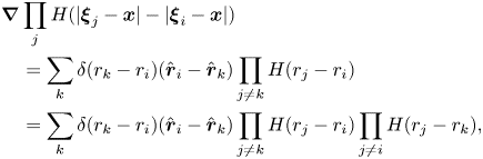 \begin{align} &\boldsymbol{\nabla} \prod_{j} H(|{\boldsymbol{\xi}}_j - \boldsymbol{x}| - |{\boldsymbol{\xi}}_i - \boldsymbol{x}| ) \nonumber\\ &\quad = \sum_k \delta(r_k - r_i) (\hat{\boldsymbol{r}}_i - \hat{\boldsymbol{r}}_k)\prod_{j {\neq} k} H(r_j- r_i) \nonumber\\ &\quad = \sum_k \delta(r_k - r_i) (\hat{\boldsymbol{r}}_i - \hat{\boldsymbol{r}}_k)\prod_{j {\neq} k} H(r_j- r_i) \prod_{j {\neq} i} H(r_j- r_k), \end{align}
where the last identity comes from the fact that  $\prod _{j {\neq} i} H(r_j- r_k)$ and $\prod _{j {\neq} i} H(r_j- r_i)$ are either 0 or 1, and $\prod _{j {\neq} i} H(r_j- r_k) = \prod _{j {\neq} k} H(r_j- r_i)$ for given $i$ and $k$, since $r_i = r_k$ as required by the $\delta$-function. Using (2.4), we have
 \begin{equation} \boldsymbol{\nabla} N_x(\boldsymbol{x}, \mathscr{F}) = \sum _i \sum_k (\hat{\boldsymbol{r}}_i - \hat{\boldsymbol{r}}_k)\delta(r_k - r_i) \prod_{j {\neq} k} H(r_j- r_i) \prod_{j {\neq} i} H(r_j- r_k) = 0, \end{equation}
the last identity comes from the exchange of indices  $i$ and $k$. This relation is in confirmation that $N_x(\boldsymbol {x}, \mathscr {F}) = 1$ almost everywhere (with the exception only in a set of zero probability). Using the first line of (A 1), the gradient of $h_i$ defined in (2.3) is
 \begin{equation} \boldsymbol{\nabla} h_i(\boldsymbol{x}, \mathscr{F}) = \sum_k \delta(r_k - r_i) (\hat{\boldsymbol{r}}_i - \hat{\boldsymbol{r}}_k) \boldsymbol{\cdot} \prod_{j {\neq} k} H(r_j- r_i). \end{equation}
Using (2.8) we have
 \begin{equation} \boldsymbol{\nabla} [\theta_c(\boldsymbol{x})P^c_{nst}(\boldsymbol{y}|\boldsymbol{x})] = \int \boldsymbol{\nabla} \left\{\chi_c(\boldsymbol{x}, \mathscr{F}) \sum_i h_i(\boldsymbol{x}, \mathscr{F}) \delta[{\boldsymbol{\xi}}_i(\mathscr{F})-{\boldsymbol{y}}] \right\} \textrm{d}\mathscr{P}. \end{equation}
Using (2.7) we have
 \begin{align} &\langle q_c\rangle_{nst}(\boldsymbol{x}, \boldsymbol{y}) \boldsymbol{\nabla} [\theta_c(\boldsymbol{x})P^c_{nst}( \boldsymbol{y}|\boldsymbol{x}) ] +\theta_c(\boldsymbol{x})P^c_{nst}(\boldsymbol{y}|\boldsymbol{x}) \boldsymbol{\nabla} \langle q_c\rangle_{nst}(\boldsymbol{x}, \boldsymbol{y}) \nonumber\\ &\quad =\int \boldsymbol{\nabla} q_c(\boldsymbol{x}, \mathscr{F}) \chi_c(\boldsymbol{x}, \mathscr{F}) \sum_i h_i(\boldsymbol{x}, \mathscr{F}) \delta({\boldsymbol{\xi}}_i-{\boldsymbol{y}})\,\textrm{d}\mathscr{P} \nonumber\\ &\qquad + \int q_c(\boldsymbol{x}, \mathscr{F}) \boldsymbol{\nabla} \left[\chi_c(\boldsymbol{x}, \mathscr{F}) \sum_i h_i(\boldsymbol{x}, \mathscr{F}) \delta({\boldsymbol{\xi}}_i-{\boldsymbol{y}})\right] \textrm{d}\mathscr{P} . \end{align}
Using (A 3), (A 4) and definition (2.7), one finds
 \begin{align} &\theta_c(\boldsymbol{x})P^c_{nst}(\boldsymbol{y}|\boldsymbol{x}) \boldsymbol{\nabla} \langle q_c\rangle_{nst}(\boldsymbol{x}, \boldsymbol{y}) = \theta_c(\boldsymbol{x})P^c_{nst}(\boldsymbol{y}|\boldsymbol{x}) \langle \nabla q_c\rangle_{nst}(\boldsymbol{x}, \boldsymbol{y}) \nonumber\\ &\quad + \int [q_c(\boldsymbol{x}, \mathscr{F}) - \langle q_c\rangle_{nst}(\boldsymbol{x}, {\boldsymbol{y}}) ] \sum_i h_i(\boldsymbol{x}, \mathscr{F}) \delta({\boldsymbol{\xi}}_i-\boldsymbol{y}) \boldsymbol{\nabla} \chi_c(\boldsymbol{x}, \mathscr{F}) \,\textrm{d}\mathscr{P} \nonumber\\ &\quad + \int [q_c(\boldsymbol{x}, \mathscr{F}) - \langle q_c\rangle_{nst}(\boldsymbol{x}, {\boldsymbol{y}}) ] \chi_c(\boldsymbol{x}, \mathscr{F}) \sum_i \delta({\boldsymbol{\xi}}_i -{\boldsymbol{y}}) \nonumber\\ &\qquad \sum_k (\hat{\boldsymbol{r}}_i - \hat{\boldsymbol{r}}_k) \delta(r_k - r_i) \prod_{j {\neq} k} H(r_j - r_i ) \,\textrm{d}\mathscr{P} . \end{align}
For the last term to be non-zero, a particle ( $k$) other than the one at ${\boldsymbol {y}}$ has to be at the same distance $r_i = |{\boldsymbol {y}} - \boldsymbol {x}|$ away from $\boldsymbol {x}$. The last term is then caused by multi-particle interactions. For randomly distributed particles with a small particle volume fraction, the particle locations are independent of each other. The probability density of having both particles $i$ and $k$ as the nearest particles to $\boldsymbol {x}$ at distance $r_k = r_i$ is proportional to $4{\rm \pi} r_k^2 P^c_{nst}(\boldsymbol {y}|\boldsymbol {x}) n_p(\boldsymbol {x}+{\boldsymbol {r}}_k)$. Furthermore, for a dispersion of identical spherical particles with radii $a$, when $|{\boldsymbol {y}} - \boldsymbol {x}| > a$, $\chi _c(\boldsymbol {x}, \mathscr {F}) = 1$, $\boldsymbol {\nabla } \chi _c(\boldsymbol {x}, \mathscr {F}) = 0$, since ${\boldsymbol {y}}$ is the nearest particle centre to position $\boldsymbol {x}$. The second term on the right-hand side then vanishes. Under these conditions, using (2.24) we have
 \begin{equation} \boldsymbol{\nabla} \langle q_c\rangle_{nst}= \langle \boldsymbol{\nabla} q_c\rangle_{nst} + O ( q_c'4 {\rm \pi}r^2 n_p ), \quad \mbox{when} \ r = |{\boldsymbol{y}}- \boldsymbol{x}|> a, \end{equation}
where  $q_c' = q_c(\boldsymbol {x},\mathscr {F}) - \langle q_c\rangle _{nst}(\boldsymbol {x}, {\boldsymbol {y}})$ is the fluctuation component of $q_c$.
A.2. For a particle quantity
Using (2.17) and noting that probability  $\mathscr{P} $ is a function of ${\boldsymbol \xi}_i$ as mentioned in § 2.1, one finds
 \begin{align} &\boldsymbol{\nabla} [n_p(\boldsymbol{x}) P_{nst}^p(\boldsymbol{y}|\boldsymbol{x}) \bar{q}_{p,nst}(\boldsymbol{x}, {\boldsymbol{y}}) ] \nonumber\\ &\quad = \int \sum_{i} q_i(\mathscr{F}) \boldsymbol{\nabla} \delta[{\boldsymbol{\xi}}_i(\mathscr{F})-\boldsymbol{x}] \sum_{j {\neq} i} h_{ij}(\mathscr{F}) \delta[{\boldsymbol{\xi}}_j(\mathscr{F})- {\boldsymbol{y}}] \,\textrm{d}\mathscr{P} \nonumber\\ &\quad={-}\int \sum_{i} q_i(\mathscr{F}) \nabla_{{\xi}_i} \delta[{\boldsymbol{\xi}}_i(\mathscr{F})- \boldsymbol{x}] \sum_{j {\neq} i} h_{ij}(\mathscr{F}) \delta[{\boldsymbol{\xi}}_j(\mathscr{F})- {\boldsymbol{y}}] \,\textrm{d}\mathscr{P} \nonumber\\ &\quad = \int \sum_{i}[ \nabla_{{\xi}_i} q_i(\mathscr{F}) ] \delta[{\boldsymbol{\xi}}_i(\mathscr{F})-\boldsymbol{x}] \sum_{j {\neq} i} h_{ij} (\mathscr{F}) \delta[{\boldsymbol{\xi}}_j(\mathscr{F})- {\boldsymbol{y}}] \,\textrm{d}\mathscr{P} \nonumber\\ &\qquad + \int \sum_{i} q_i(\mathscr{F}) \delta[{\boldsymbol{\xi}}_i(\mathscr{F})-\boldsymbol{x}] \nabla_{{\xi}_i} \left\{\sum_{j {\neq} i} h_{ij}(\mathscr{F}) \delta[{\boldsymbol{\xi}}_j(\mathscr{F})- {\boldsymbol{y}}]\,\textrm{d}\mathscr{P}\right\}. \end{align}
 Setting  $q_i = 1$, then $\bar {q}_{p,nst}(\boldsymbol {x}, {\boldsymbol {y}}) =1$, we have
 \begin{equation} \boldsymbol{\nabla} [n_p(\boldsymbol{x}) P_{nst}^p(\boldsymbol{y}|\boldsymbol{x}) ] = \int \sum_{i} \delta({\boldsymbol{\xi}}_i -\boldsymbol{x}) \nabla_{{\xi}_i} \left\{\sum_{j {\neq} i} h_{ij}(\mathscr{F}) \delta({\boldsymbol{\xi}}_j -{\boldsymbol{y}})\,\textrm{d}\mathscr{P}\right\}.\end{equation}
Multiplying this equation by  $\bar {q}_{p,nst}(\boldsymbol {x}, {\boldsymbol {y}})$ and subtracting the result from (A 8), after using (2.17) we find
 \begin{align} &n_p(\boldsymbol{x}) P_{nst}^p(\boldsymbol{y}|\boldsymbol{x}) \boldsymbol{\nabla} \bar{q}_{p,nst}(\boldsymbol{x}, {\boldsymbol{y}}) = n_p(\boldsymbol{x}) P_{nst}^p(\boldsymbol{y}|\boldsymbol{x}) \overline{\nabla_{{\xi}_i} q_i}(\boldsymbol{x}, {\boldsymbol{y}}) \nonumber\\ &\quad + \int \sum_{i} [q_i(\mathscr{F}) - \bar{q}_{p,nst}(\boldsymbol{x}, {\boldsymbol{y}})] \delta({\boldsymbol{\xi}}_i -\boldsymbol{x}) \sum_{j {\neq} i} h_{ij}(\mathscr{F}) \delta({\boldsymbol{\xi}}_j - {\boldsymbol{y}}) \nabla_{{\xi}_i} \,\textrm{d}\mathscr{P} \nonumber\\ &\quad + \int \sum_{i} [q_i(\mathscr{F}) - \bar{q}_{p,nst}(\boldsymbol{x}, {\boldsymbol{y}})] \delta({\boldsymbol{\xi}}_i -\boldsymbol{x}) \delta({\boldsymbol{\xi}}_j - {\boldsymbol{y}}) \nabla_ {{\xi}_i}\sum_{j {\neq} i} h_{ij}(\mathscr{F}) \,\textrm{d}\mathscr{P}. \end{align}
For finite size particles, the second term  $ \delta ({\boldsymbol {\xi }}_j- {\boldsymbol {y}})\nabla_{\xi_i}\,\textrm{d} \mathscr{P}$ represents the effect of particle $i$ position on particle $j$ position. For a dilute particle dispersion this terms is of order $n_p^2$. Similar to (A 8) the last term represents multi-particle effects, and is also of order $n_p^2$ in a dilute particle dispersion. Noting that on the left-hand side $n_pP_{nst}^p$ is also of order $n_p^2$; therefore, for a particle quantity, we have $\boldsymbol {\nabla } \bar {q}_{p,nst} - \overline {\nabla _{{\xi }_i} q_i} = O(1)$, in contrast to (A 7) for a continuous phase quantity.
Appendix B
In this appendix, we consider Stokes flows in particle suspensions driven by body forces acting on the particles and the fluid. Since Stokes flow equations are linear, different types of forces can be considered separately. Their combined effect can be obtained easily by superposition. Without loss of generality, we can only consider the gravity.
We calculate the conditionally averaged velocity  $\langle {\boldsymbol {v}}_c\rangle _{nst}(\boldsymbol {x}, {\boldsymbol {y}})$ in the effective medium shown on the right-hand side of figure 2. According to definition (2.7), $\langle {\boldsymbol {v}}_c\rangle _{nst}(\boldsymbol {x}, {\boldsymbol {y}})$ is the velocity of the continuous phase at $\boldsymbol {x}$ averaged under the condition that $\boldsymbol {x}$ is in the fluid phase and that ${\boldsymbol {y}}$ is the nearest particle centre to $\boldsymbol {x}$. To calculate the velocity, we now introduce the pressure $\langle p\rangle _{nst}({\boldsymbol {z}}|\boldsymbol {x}, {\boldsymbol {y}})$ and the mixture velocity $\langle {\boldsymbol {v}}_m\rangle _{nst}({\boldsymbol {z}}|\boldsymbol {x}, {\boldsymbol {y}})$ at a generic point ${\boldsymbol {z}}$, as shown on the right-hand side of figure 2, averaged under the condition that $\boldsymbol {x}$ is occupied by the fluid and that ${\boldsymbol {y}}$ is the centre of the nearest particle to $\boldsymbol {x}$. Clearly, $\langle {\boldsymbol {v}}_c\rangle _{nst}(\boldsymbol {x}, {\boldsymbol {y}}) = \langle {\boldsymbol {v}}_m\rangle _{nst}(\boldsymbol {x}|\boldsymbol {x}, {\boldsymbol {y}})$, because $\boldsymbol {x}$ is in the particle-free region.
Let  $\rho _p$ and $\rho _c$ be densities of the particle and the fluid. Outside the particle-free region ( $|{\boldsymbol {z}} - \boldsymbol {x}| > R = |{\boldsymbol {y}} - \boldsymbol {x}|$), the medium has an effective density $\theta _p\rho _p +(1-\theta _p) \rho _c$. In this medium, particle velocity fluctuations (Guazzelli & Hinch Reference Guazzelli and Hinch2011) are not restricted by external mechanisms. The Stokes equation for the mixture becomes
 \begin{align} &-\boldsymbol{\nabla} \langle p\rangle_{nst}({\boldsymbol{z}}|\boldsymbol{x}, {\boldsymbol{y}}) + \mu \nabla^2 \langle{\boldsymbol{v}}_m\rangle_{nst}({\boldsymbol{z}}|\boldsymbol{x}, {\boldsymbol{y}}) \nonumber\\ &\quad = H(R-|{\boldsymbol{z}} - \boldsymbol{x}|) \theta_p (\rho_p-\rho_c){\boldsymbol{g}} -[\theta_p\rho_p +(1-\theta_p) \rho_c]{\boldsymbol{g}}, \end{align}
where  ${\boldsymbol {g}}$ is the acceleration due to gravity. In this equation, we have only considered force monopoles and neglected other $O(\theta _p)$ terms because these force monopoles are the leading contributors of the long-range effects. This equation is (7.4) of Hinch (Reference Hinch1977) with only the first three terms on the left-hand side kept, and $3a$ in the fourth terms replaced by $R$. This difference in terms only cause an $O(\theta _p)$ correction to the velocity solution (Hinch Reference Hinch1977), while for our purpose, as shown in the main text, only the velocity correct to $O(1)$ is needed. We consider these $O(\theta _p)$ terms in (B 1) to ensure they do not cause a larger $O(1)$ effect on the averaged velocities ${\boldsymbol {V}}'$ and $\langle {\boldsymbol {v}}_c\rangle$, since an $O(\theta _p)$ term in the equation does not necessarily result in the same order contributions to the average velocities. As shown in the main text, the contributions to the velocities from these terms are $O(\theta _p^{1/3})$.
The last term on the right-hand side of (B 1) can be accommodated by a constant pressure gradient without a consequence for the velocity. The velocity contribution from the first term on the right-hand side of (B 1) can be calculated as
 \begin{equation} {\boldsymbol{v}}_b ({\boldsymbol{z}}|\boldsymbol{x}, {\boldsymbol{y}}) = \theta_p {\rm \Delta} \rho {\boldsymbol{g}}\boldsymbol{\cdot} \int_{|\boldsymbol{x}' - \boldsymbol{x}|<|{\boldsymbol{y}} - \boldsymbol{x}| } {\boldsymbol{S}} ({\boldsymbol{r}}') \,\textrm{d}^3x', \quad {\boldsymbol{r}}' = \boldsymbol{x}' - {\boldsymbol{z}}, \end{equation}
where  ${\rm \Delta} \rho = \rho _p-\rho _c$, the integration volume is the particle-free region centred at $\boldsymbol {x}$ as shown in figure 2, and ${\boldsymbol {S}} ({\boldsymbol {r}})$ is the Stokeslet,
 \begin{equation} {\boldsymbol{S}} ({\boldsymbol{r}}) ={-}\frac{1}{8 {\rm \pi}\mu}\left( \frac{\boldsymbol{I}}{r} + \frac{{\boldsymbol{r}} {\boldsymbol{r}} }{r^3}\right). \end{equation}
For a specified  ${\boldsymbol {y}}$ at a large $r = |{\boldsymbol {z}}-\boldsymbol {x}|\gg R= |{\boldsymbol {y}}-\boldsymbol {x}|$, ${\boldsymbol {v}}_b ({\boldsymbol {z}}|\boldsymbol {x}, {\boldsymbol {y}})$ decays as $O(n_pR^3/r)$. At the centre of the particle free region, with ${\boldsymbol {z}} = \boldsymbol {x}$, ${\boldsymbol {v}}_b (\boldsymbol {x}, {\boldsymbol {y}}) = {\boldsymbol {v}}_b (\boldsymbol {x}|\boldsymbol {x}, {\boldsymbol {y}})= -({R^2}/{3\mu })\theta _p{\rm \Delta} \rho {\boldsymbol {g}}$.
With solution (B 2), the approximation of the conditionally averaged velocity for a generic position  ${\boldsymbol {z}}$ can be constructed as
 \begin{align} \langle {\boldsymbol{v}}_m\rangle_{nst} ({\boldsymbol{z}}|\boldsymbol{x}, {\boldsymbol{y}}) &= {\boldsymbol{v}}_0 +\left[\bar{{\boldsymbol{v}}}_p - {\boldsymbol{v}}_0-{\boldsymbol{v}}_b ({\boldsymbol{y}}|\boldsymbol{x}, {\boldsymbol{y}}) \right] \left(\frac{3a}{4r}+\frac{a^3}{4r^3} \right) \nonumber\\ &\quad + \frac{\boldsymbol{r}}{r} \left\{\frac{\boldsymbol{r}}{r}\boldsymbol{\cdot}\left[\bar{{\boldsymbol{v}}}_p -{\boldsymbol{v}}_0 -{\boldsymbol{v}}_b ({\boldsymbol{y}}|\boldsymbol{x}, {\boldsymbol{y}})\right]\right\}\left(\frac{3a}{4r}- \frac{3a^3}{4r^3} \right) \nonumber\\ &\quad + {\boldsymbol{v}}_b ({\boldsymbol{z}}|\boldsymbol{x}, {\boldsymbol{y}}) , \quad {\boldsymbol{r}} = {\boldsymbol{z}} - {\boldsymbol{y}}, \end{align}
since the first three terms with the corresponding solution for the pressure satisfy the Stokes equation, ((B 1) with the right-hand side set to zero), and  ${\boldsymbol {v}}_b ({\boldsymbol {z}}|\boldsymbol {x}, {\boldsymbol {y}})$ is obtained from (B 2) satisfying (B 1) because of the Stokeslet. At the centre of the particle free region, ${\boldsymbol {z}} = \boldsymbol {x}$, this relation becomes (3.8) with ${\boldsymbol {v}}_b (\boldsymbol {x}, {\boldsymbol {y}}) = {\boldsymbol {v}}_b (\boldsymbol {x}|\boldsymbol {x}, {\boldsymbol {y}})$ and ${\boldsymbol {v}}_b' = {\boldsymbol {v}}_b ({\boldsymbol {y}}|\boldsymbol {x}, {\boldsymbol {y}})$ in (3.7).
This approximation implies the nearest particle at  ${\boldsymbol {y}}$ experiences the background fluid velocity ${\boldsymbol {v}}_0+{\boldsymbol {v}}_b ({\boldsymbol {y}}|\boldsymbol {x}, {\boldsymbol {y}})$ while satisfying the boundary condition $\langle {\boldsymbol {v}}_m\rangle _{nst} (\infty |\boldsymbol {x}, {\boldsymbol {y}}) = {\boldsymbol {v}}_0$. On the surface ${\boldsymbol {z}} = {\boldsymbol {y}} + a {\boldsymbol {n}}$ of the particle at ${\boldsymbol {y}}$, where ${\boldsymbol {n}}$ is the unit outward normal, there is an error ${\boldsymbol {v}}_b ({\boldsymbol {y}}+ a {\boldsymbol {n}}|\boldsymbol {x}, {\boldsymbol {y}}) - {\boldsymbol {v}}_b ({\boldsymbol {y}}|\boldsymbol {x}, {\boldsymbol {y}}) = O(a \boldsymbol {\nabla }{\boldsymbol {v}}_b ({\boldsymbol {y}}|\boldsymbol {x}, {\boldsymbol {y}})) = O(n_p aR)$ in satisfying the no-slip boundary condition, since $\nabla$ is of $O(1/R)$. This error is small compared with ${\boldsymbol {v}}_b ({\boldsymbol {y}}|\boldsymbol {x}, {\boldsymbol {y}}) = O(n_p R^2)$, since $a < R$.
Although only the gravity is considered above, the calculation can be generalized if other uniform external force fields are used to maintain a specified average particle velocity. For instance, for electric fields, densities  $\rho _p$ and $\rho _c$ above can be regarded as the charge densities, and ${\boldsymbol {g}}$ can be replaced with the electric field ${\boldsymbol {E}}$. In this case, solution (B 4) remains valid; therefore, the force (3.23) in the main text is independent of the external force acting on the dilute dispersion.


 Open access