


1. Introduction
The manuscript considers unsteady and turbulent channel flows of non-Newtonian viscoelastic and elastoviscoplastic fluids. The dynamics of non-Newtonian turbulence has attracted a growing interest due to numerous industrial applications dealing with non-Newtonian fluids. Real industrial and natural fluids often present several non-Newtonian effects at the same time, such as plasticity (yield stress) and elasticity. Turbulent flows of yield-stress fluids are found in several industries such as petroleum, paper, mining and sewage treatment (Hanks Reference Hanks1963, Reference Hanks1967; Maleki & Hormozi Reference Maleki and Hormozi2018). Highly inertial flows of elastoviscoplastic fluids can also be found in geophysical applications, such as mudslides and the tectonic dynamics of the Earth (Oishi, Martins & Thompson Reference Oishi, Martins and Thompson2017).
Yield-stress fluids behave like solids below a local stress threshold, and flow like liquids above this threshold. Assuming that the material is a rigid solid at stresses lower than the yield stress, purely viscoplastic models are obtained, such as the Bingham model (Bingham Reference Bingham1922), where the solvent viscosity of the yielded fluid flow follows a Newtonian law, and the Herschel–Bulkley model (Herschel & Bulkley Reference Herschel and Bulkley1926), where the yielded fluid flow is shear thinning. However, many yield-stress fluids deform like elastic solids in the unyielded state and behave as viscoelastic liquids in the yielded state, displaying elastic ( $E$), viscous (
 $V$) and plastic (
 $P$) properties.
A simple dynamic elastoviscoplastic (EVP) constitutive model that can be integrated with direct numerical simulations was proposed by Saramito (Reference Saramito2007). The model has proven to capture viscoplastic and elastic effects (Cheddadi et al. Reference Cheddadi, Saramito, Dollet, Raufaste and Graner2011; Fraggedakis, Dimakopoulos & Tsamopoulos Reference Fraggedakis, Dimakopoulos and Tsamopoulos2016) and to properly match experimental results and observations (Holenberg et al. Reference Holenberg, Lavrenteva, Shavit and Nir2012) (common materials used to study this type of EVP fluids are Carbopol solutions and liquid foams Firouznia et al. Reference Firouznia, Metzger, Ovarlez and Hormozi2018; Zade et al. Reference Zade, Shamu, Lundell and Brandt2020). The model was extended by the same author to account for shear-thinning effects (Saramito Reference Saramito2009), combining the Oldroyd viscoelastic model with the Herschel–Bulkley viscoplastic model, with a power-law index that allows a shear-thinning behaviour in the yielded state. When the index is equal to unity, the model reduces to the one proposed in his previous work, i.e. Saramito (Reference Saramito2007). Apart from the models proposed by Saramito, many other EVP models exist in the literature. The interested reader is referred to Crochet & Walters (Reference Crochet and Walters1983), Balmforth, Frigaard & Ovarlez (Reference Balmforth, Frigaard and Ovarlez2014), Saramito (Reference Saramito2016) and Saramito & Wachs (Reference Saramito and Wachs2017) for a thorough review of models and numerical methods.
Turbulent flow of purely viscoelastic fluids has gained attention in the drag-reduction and flow control communities, since a tiny amount of polymer (parts per million) has proven efficient in reducing friction drag in pipe flows (Virk Reference Virk1971). Drag reduction by polymers is related to their ability to modify coherent structures in wall-bounded turbulence (Dubief et al. Reference Dubief, White, Terrapon, Shaqfeh, Moin and Lele2004, Reference Dubief, Terrapon, White, Shaqfeh, Moin and Lele2005). Polymers influence the turbulent cycle in two ways: they attenuate near-wall vortices, but at the same time they also increase the streamwise kinetic energy of the near-wall streaks. The net balance of these two opposite actions leads to a self-sustained drag-reduced turbulent flow. More recently, Xi & Graham (Reference Xi and Graham2010, Reference Xi and Graham2012a,Reference Xi and Grahamb) proposed that polymeric drag reduction is a time-dependent process: turbulent flows with polymers spend relatively more time in hibernating phases, where the turbulence is weak, and less time in active phases with strong turbulence. The turbulent coherent structures, streamwise vortices and streaks, were found to differ in appearance depending on whether the flow was in an active or a hibernating phase. Biancofiore, Brandt & Zaki (Reference Biancofiore, Brandt and Zaki2017) examined the secondary instability of streaks in viscoelastic flows, showing that the streaks reach a lower average energy with increasing elasticity due to a resistive polymer torque that opposes the streamwise vorticity and, as a result, opposes the lift-up mechanism. Numerous studies have addressed the topic of polymeric drag reduction and all cannot be reviewed here for brevity; the interested reader is referred to White & Mungal (Reference White and Mungal2008) for a thorough introduction to this subject.
Turbulent flow of yield-stress fluids (plasticity) has been studied much less, despite its relevance for applications. The reason is twofold. Time-resolved measurements in yield-stress fluids are very challenging, even in laminar flows. Most real-life yield-stress fluids are opaque and hence do not provide optical access. The transparent laboratory fluid Carbopol, often used in these experiments, needs careful preparation to achieve well-controlled properties (Dinkgreve, Fazilati & Bonn Reference Dinkgreve, Fazilati, Denn and Bonn2018; Tabuteau, Coussot & De Bruyn Reference Tabuteau, Coussot and De Bruyn2018), and exhibits slip on smooth surfaces that needs to be avoided or carefully controlled (Firouznia et al. Reference Firouznia, Metzger, Ovarlez and Hormozi2018). On the other hand, direct numerical simulations of yield-stress fluids have not been affordable until recently. Rosti et al. (Reference Rosti, Izbassarov, Tammisola, Hormozi and Brandt2018a) first studied the turbulent channel flow of a yield-stress fluid in a near-viscoplastic limit using the Saramito EVP model (Saramito Reference Saramito2007), adding a tiny amount of elasticity to achieve numerical stability (the Weissenberg number was  $Wi=0.01$). When the Bingham number was gradually increased from zero, the flow became less turbulent and more correlated in the streamwise direction, until it completely relaminarised at
  $Bi=2.8$. The velocity correlations revealed that the size and length of the near-wall streaks increased with the Bingham number. The friction factor decreased with the Bingham number in the turbulent regime, while it increased with the same in the laminar regime. Le Clainche et al. (Reference Le Clainche, Izbassarov, Rosti, Brandt and Tammisola2020) analysed further the simulation data of Rosti et al. (Reference Rosti, Izbassarov, Tammisola, Hormozi and Brandt2018a) using high-order dynamic mode decomposition, and compared the modes with those in Newtonian fluids, and also in purely viscoelastic fluids. Their results indicated that elasticity and plasticity have similar effects on the coherent structures; in both cases, the flow is dominated by long streaks disrupted by rapid, localised perturbations. The Newtonian flow, on the other hand, displays short streaks and a more chaotic dynamics. Very recent experiments in a duct flow of Carbopol confirmed that the energy content at low wavenumbers and streamwise anisotropy were higher than in Newtonian turbulence (Mitishita et al. Reference Mitishita, MacKenzie, Elfring and Frigaard2021), indicating that streamwise near-wall structures (streaks) were enhanced in Carbopol. These experiments at higher Reynolds numbers also confirmed the qualitative changes that viscoplasticity causes in mean flow profiles and Reynolds stresses, as observed by Rosti et al. (Reference Rosti, Izbassarov, Tammisola, Hormozi and Brandt2018a).
In addition, many earlier direct numerical simulation studies addressed the turbulence in Bingham pseudoplastic fluids (obtained by regularising the Bingham model by a large viscosity) (Rudman & Blackburn Reference Rudman and Blackburn2006; Guang et al. Reference Guang, Rudman, Chryss, Slatter and Bhattacharya2011; Zhu et al. Reference Zhu, Yu, Shao and Deng2020), and their shear-thinning version, regularised Herschel–Bulkley fluids by Rudman et al. (Reference Rudman, Blackburn, Graham and Pullum2004) and Singh, Rudman & Blackburn (Reference Singh, Rudman and Blackburn2017). Very recently, Zhu et al. (Reference Zhu, Yu, Shao and Deng2020) studied the turbulence of a Bingham pseudoplastic fluid in a vertical channel with particles, at a higher bulk Reynolds number ( $Re_b=8000$) than Rosti et al. (Reference Rosti, Izbassarov, Tammisola, Hormozi and Brandt2018a). They also obtained a drag reduction with an increasing Bingham number, along with an increasing streamwise coherence of the flow structures and observed that the turbulent statistics were asymmetric with respect to the centreline at higher Bingham numbers.
Transitional flows of yield-stress fluids in pipes and channels have been addressed in many studies, both experimentally and computationally. An asymmetric mean flow profile is a characteristic feature observed in pipe flow experiments of yield-stress fluids (Escudier et al. Reference Escudier, Poole, Presti, Dales, Nouar, Desaubry, Graham and Pullum2005; Peixinho et al. Reference Peixinho, Nouar, Desaubry and Théron2005; Esmael & Nouar Reference Esmael and Nouar2008; Guzel, Frigaard & Martinez Reference Guzel, Frigaard and Martinez2009), and for fluids with a Herschel–Bulkley-type rheology (Escudier & Presti Reference Escudier and Presti1996). According to Esmael & Nouar (Reference Esmael and Nouar2008), this was caused by an asymmetric nonlinear coherent structure consisting of two counter-rotating vortices. Experiments on laminar steady flow of a yield-stress fluid in a duct laden with particles were performed recently by Zade et al. (Reference Zade, Shamu, Lundell and Brandt2020). Computational studies on transitional flows have mainly focused on the linear and nonlinear stability of channel flows (Frigaard, Howison & Sobey Reference Frigaard, Howison and Sobey1994; Nouar & Frigaard Reference Nouar and Frigaard2001; Frigaard & Nouar Reference Frigaard and Nouar2003; Nouar et al. Reference Nouar, Kabouya, Dusek and Mamou2007; Metivier, Nouar & Brancher Reference Metivier, Nouar and Brancher2010; Nouar & Bottaro Reference Nouar and Bottaro2010; Bentrad et al. Reference Bentrad, Esmael, Nouar, Lefevre and Ait-Messaoudene2017). Most importantly, within the Bingham model, the central plug regions of a channel flow remain unyielded despite linear perturbations, and hence the flow is always linearly stable. In non-modal analysis, in contrast to Newtonian fluids, the optimal disturbance is found to be an oblique wave (Nouar et al. Reference Nouar, Kabouya, Dusek and Mamou2007), associated with the lift-up effect (Schmid Reference Schmid2007; Brandt Reference Brandt2014). However, Nouar & Bottaro (Reference Nouar and Bottaro2010) found that a slightly perturbed mean flow profile supports exponential amplification of streamwise-travelling waves, indicating another possible transition scenario for the plane channel flow of a yield-stress fluid.
Concluding, all previous studies on EVP turbulence focused on either purely viscoelastic or near-viscoplastic fluids. The questions remain as to what happens when both elasticity and plasticity effects are finite and interact with each other. The recent experimental study by Mitishita et al. (Reference Mitishita, MacKenzie, Elfring and Frigaard2021) also raised the question of how the findings of Rosti et al. (Reference Rosti, Izbassarov, Tammisola, Hormozi and Brandt2018c) would be affected by finite elasticity. The present study focuses on EVP fluids at finite Weissenberg numbers, i.e. fluids with finite viscoelasticity and yield stress.
In this work, we perform direct numerical simulations of turbulent channel flows of an incompressible EVP fluid and extend the one by Rosti et al. (Reference Rosti, Izbassarov, Tammisola, Hormozi and Brandt2018c) by considering a wide range of Weissenberg numbers  $0\le Wi \le 16$ and Bingham numbers
  $0 \le Bi \le 22.4$, all at the bulk Reynolds number
  $Re = 2800$. The non-Newtonian flow is simulated by solving the full unsteady incompressible Navier–Stokes equations coupled with a modified version of the model proposed by Saramito (Reference Saramito2007) for the evolution of the additional EVP stress tensor.
The manuscript is organised as follows. In § 2, we first discuss the flow configuration and the governing equations, and then present the numerical methodology used. The new model with some test cases is reported in § 2.1, while the new results are presented in § 3. In particular, we discuss the role of elasticity and plasticity on a turbulent channel flow. Finally, a summary of the main findings and conclusions are collected in § 5.
2. Formulation
We consider the laminar and turbulent flows of an incompressible EVP fluid through a plane channel with two impermeable rigid walls. Figure 1(a) shows a sketch of the geometry and the Cartesian coordinate system, where  $x$,
$x$,  $y$ and
  $z$ (
$z$ ( $x_1$,
  $x_2$ and
  $x_3$) denote the streamwise, wall-normal and spanwise coordinates, while
  $u$,
$u$,  $v$ and
  $w$ (
$w$ ( $u_1$,
  $u_2$ and
  $u_3$) denote the respective components of the velocity field. The lower and upper stationary impermeable walls are located at
  $y=0$ and
  $2h$, respectively, where
  $h$ represents the channel half-height.

Figure 1. Sketch of the computational domain. The  $XY$ and
  $ZY$ planes in the middle of the domain show instantaneous streamwise velocity contours with the scale ranging from 0 (blue) to 1.27
 $U_b$ (red), where
  $U_b$ denotes the bulk velocity. Green structures represent unyielded regions.
The fluid motion is governed by the conservation of momentum and the incompressibility constraint
 $$\begin{gather} \frac{\partial u_i}{\partial t} + \frac{\partial u_i u_j}{\partial x_j} = \frac{1}{\rho} \frac{\partial \sigma_{ij}}{\partial x_j}, \end{gather}$$
 $$\begin{gather}\frac{\partial u_i}{\partial x_i} = 0, \end{gather}$$
where  $\rho$ is the fluid density and
  $\sigma _{ij}$ the total Cauchy stress tensor, which is written as
  $\sigma _{ij} = -p \delta _{ij} + 2 \mu _f D_{ij} + \tau _{ij}$, where
  $p$ is the pressure,
  $\mu _f$ the fluid molecular dynamic viscosity (also called solvent viscosity),
  $\delta$ the Kronecker delta and
  $D_{ij}$ the strain rate tensor defined as
  $D_{ij}=( \partial u_i / \partial x_j + \partial u_j / \partial x_i )/2$. The additional EVP stress tensor
  $\tau _{ij}$ accounts for the non-Newtonian behaviour of the fluid, here described by a modified version of the model proposed by Saramito (Reference Saramito2007). In the original model, when the stress
  $\sigma$ is below the yield stress
  $\tau _0$, the system predicts only recoverable Kelvin–Voigt viscoelastic deformations, while when the stress exceeds the yield value
  $\tau _0$, the fluid behaves as an Oldroyd-B viscoelastic fluid. Thus, the total strain rate
  $\dot {\varepsilon }$ is shared between an elastic contribution
  $\dot {\varepsilon }_e$ and a plastic one
  $\dot {\varepsilon }_p$ (Cheddadi et al. Reference Cheddadi, Saramito, Dollet, Raufaste and Graner2011). Since the Oldroyd-B model assumes infinitely stretched dumbbells, the range of application of the model is limited to low elasticity. To overcome this drawback, we instead use the finite extensible nonlinear elastic-Peterlin (FENE-P) model. Thus, the instantaneous values of all the components of the stress tensor
  $\tau _{ij}$ are found by solving the following transport equation:
 \begin{align} &\lambda \left( \frac{\partial \tau_{ij}}{\partial t} + \frac{\partial u_k \tau_{ij}}{\partial x_k} - \tau_{kj}\frac{\partial u_i}{\partial x_k} - \tau_{ik}\frac{\partial u_j}{\partial x_k} \right) + F f \tau_{ij} \nonumber\\ &\quad -\left(\frac{\partial \ln F}{\partial t}+\frac{\partial u_k \ln F}{\partial x_k}\right)(\lambda \tau_{ij}+\mu_m\delta_{ij})= 2 \mu_m D_{ij}, \end{align}
where
 \begin{equation} F=1+ \frac{\left(3+ \dfrac{\lambda}{\mu_m}\tau_{ii}\right)}{L^2}, \quad f=\max \left(0, \frac{ \vert \tau_d \vert - \tau_0}{\vert \tau_d \vert} \right). \end{equation}
Here,  $\lambda$ is the relaxation time,
  $\mu _m$ is an additional viscosity,
  $L$ is the maximum polymer extensibility,
  $\tau _0$ the yield stress and
  $\vert \tau _d \vert$ represents the second invariant of the deviatoric part of the added stress tensor. The EVP parameters
  $\mu _f$,
  $\mu _m$,
  $\lambda$ and
  $\tau _0$ can be obtained by experimental data following the procedure detailed by Fraggedakis et al. (Reference Fraggedakis, Dimakopoulos and Tsamopoulos2016), based on the determination of the linear material functions, i.e. the storage modulus
  $G'$ and the loss modulus
  $G''$. The above constitutive equation gives a Kelvin–Voigt solid in the limit
  $F\approx 1$, which is the case in the unyielded state, and a behaviour like a FENE-P fluid in the yielded state. The previous equation can be rewritten in terms of the conformation tensor
  $C_{ij}$ as
 \begin{equation} \frac{\partial C_{ij}}{\partial t} + \frac{\partial u_k C_{ij}}{\partial x_k} - C_{kj}\frac{\partial u_i}{\partial x_k} - C_{ik}\frac{\partial u_j}{\partial x_k} ={-}\frac{f}{\lambda} (F C_{ij} - \delta_{ij}), \end{equation}
where the EVP stress tensor  $\tau _{ij}$ is related to the conformation tensor by the relation
 \begin{equation} \tau_{ij}=\frac{\mu_m}{\lambda}(F C_{ij} - \delta_{ij}). \end{equation}
We use the log conformation method to overcome the well-known high Weissenberg number problem (Fattal & Kupferman Reference Fattal and Kupferman2004; Hulsen, Fattal & Kupferman Reference Hulsen, Fattal and Kupferman2005; Izbassarov & Muradoglu Reference Izbassarov and Muradoglu2015; De Vita et al. Reference De Vita, Rosti, Izbassarov, Duffo, Tammisola, Hormozi and Brandt2018). In this approach, (2.4) is rewritten in terms of the logarithm of the conformation tensor through an eigen-decomposition, i.e.  $\boldsymbol {\varPsi }=\log \boldsymbol {C}$, which ensures the positive definiteness of the conformation tensor. The core feature of the formulation is the decomposition of the gradient of the divergence free velocity field
  $\partial u_j / \partial x_i$ into two anti-symmetric tensors,
  $\varOmega _{ij}$ (pure rotation) and
  $N_{ij}$, and into a symmetric tensor,
  $B_{ij}$, which commutes with the conformation tensor, i.e.
 \begin{equation} \frac{\partial u_j}{\partial x_i} = \varOmega_{ij} + B_{ij} + N_{ij}C_{ji}. \end{equation}
The modified transport equation to be solved is thus
 \begin{equation} \frac{\partial \varPsi_{ij}}{\partial t} + \frac{\partial u_k \varPsi_{ij}}{\partial x_k} - (\varOmega_{ik} \varPsi_{kj} - \varPsi_{ik} \varOmega_{kj}) - 2B_{ij} = \frac{f}{\lambda} ((\textrm{e}^{-\varPsi})_{ij} - F \delta_{ij} ). \end{equation}
Once this equation is solved, the conformation tensor can be obtained using the inverse transformation  $\boldsymbol {C} = \textrm {e}^{\boldsymbol {\varPsi }}$.
Finally, the full system of equations can be rewritten in a non-dimensional form as
 $$\begin{gather} Re \left( \frac{\partial u_i}{\partial t} + \frac{\partial u_i u_j}{\partial x_j} \right) = \frac{\partial}{\partial x_j} ({-}p \delta_{ij} + 2 \beta D_{ij} + \tau_{ij}), \end{gather}$$
 $$\begin{gather}\frac{\partial u_i}{\partial x_i} = 0, \end{gather}$$
 $$\begin{gather}\frac{\partial \varPsi_{ij}}{\partial t} + \frac{\partial u_k \varPsi_{ij}}{\partial x_k} - \left( \varOmega_{ik} \varPsi_{kj} - \varPsi_{ik} \varOmega_{kj} \right) - 2B_{ij} = \frac{f}{Wi} ((\textrm{e}^{-\varPsi})_{ij} - F \delta_{ij}), \end{gather}$$
 $$\begin{gather}F =1+ \frac{\left(3+ \dfrac{Wi}{1-\beta}\tau_{ii}\right)}{L^2}, \quad f =\max \left(0, \frac{ \vert \tau_d \vert - Bi}{\vert \tau_d \vert} \right), \end{gather}$$
 $$\begin{gather}\tau_{ij}=\frac{(1-\beta)}{Wi}(F(\textrm{e}^{\varPsi})_{ij} - \delta_{ij}),\end{gather}$$
where we have used the same symbols to define the non-dimensional variables for simplicity. Four non-dimensional numbers appear in the previous set of equations: the Reynolds number  $Re$, the Weissenberg number
  $Wi$, the Bingham number
  $Bi$ and the viscosity ratio
  $\beta$, defined as
  $Re = \rho U \mathcal {L} / \mu _0$,
  $Bi = \tau _0 \mathcal {L} / \mu _0 U$,
  $Wi = \lambda U / \mathcal {L}$ and
  $\beta =\mu _f/\mu _0$, where
  $U$ and
  $\mathcal {L}$ are a characteristic velocity and length scales of the flow,
  $\rho$ the fluid density and
  $\mu _0$ the total viscosity, i.e.
  $\mu _0=\mu _f+\mu _m$.
The equations of motion are solved with an extensively validated in-house code (Rosti & Brandt Reference Rosti and Brandt2017; De Vita et al. Reference De Vita, Rosti, Izbassarov, Duffo, Tammisola, Hormozi and Brandt2018; Izbassarov et al. Reference Izbassarov, Rosti, Niazi Ardekani, Sarabian, Hormozi, Brandt and Tammisola2018; Rosti et al. Reference Rosti, Izbassarov, Tammisola, Hormozi and Brandt2018c; Alghalibi, Rosti & Brandt Reference Alghalibi, Rosti and Brandt2019; Shahmardi et al. Reference Shahmardi, Zade, Ardekani, Poole, Lundell, Rosti and Brandt2019). The governing equations are discretised with the second-order centred finite difference scheme on a staggered uniform grid, except for the advection term in (2.7) where the fifth-order WENO (weighted essentially non-oscillatory) scheme is adopted (Shu Reference Shu2009; Sugiyama et al. Reference Sugiyama, Ii, Takeuchi, Takagi and Matsumoto2011). The time integration is performed with a fractional-step method (Kim & Moin Reference Kim and Moin1985) and a third-order explicit Runge–Kutta scheme except for the EVP stress term which is advanced with the Crank–Nicolson method.
In all the simulations, periodic boundary conditions are used in the streamwise and spanwise directions, while the no-slip and no-penetration boundary conditions are enforced on the solid walls. For all the turbulent cases considered hereafter with a bulk Reynolds number equal to  $Re_b=2800$, the equations of motion are discretised by using
  $1728 \times 576 \times 864$ grid points on a computational domain of size
  $6h \times 2h \times 3h$ in the streamwise, wall-normal and spanwise directions, with the resolution satisfying the constraint
  $\Delta x^{+} = \Delta y^{+} = \Delta z^{+} < 0.6$, where the superscript
  $^+$ indicates the wall units. The spatial resolution has been chosen equal to the one used in a previous work (Rosti et al. Reference Rosti, Izbassarov, Tammisola, Hormozi and Brandt2018a) in order to properly resolve the turbulent scales as well as the unyielded plug regions which form intermittently in the domain, and verified a posteriori with a grid refinement study. In the low Reynolds fully laminar cases, the spatial resolution was relaxed and the domain size in the homogeneous directions reduced. Finally, all the turbulent cases are initialised with a fully developed channel flow with zero EVP stress (
 $\tau _{ij}=0$); after the flow and stresses have reached a statistically steady state, the calculations are continued for an interval of approximately
  $500$ bulk time units, during which the statistics are computed.
2.1. Validations of the FENE-P-based EVP model
The present implementation for single and multiphase flows of an EVP fluid has been extensively validated in the past; here, we report further test cases of the new FENE-P-based EVP model also to present its rheological behaviour.
First, we consider a three-dimensional uniaxial elongational flow, with a constant elongational rate  $\dot {\epsilon }_0$: the Weissenberg number
  $Wi=\lambda \dot {\epsilon }_0$ and extensibility parameter
  $L^2$ are varied in the range of
  $0.25 \le Wi \le 0.75$ and
  $10\le L^2 \le \infty$, respectively, while the Bingham number
  $Bi=\tau _0/(\mu _0 \dot {\epsilon _0})=1$ and the viscosity ratio
  $\beta =0$. The fluid flow is assumed to have a constant velocity gradient
  $\partial u_i / \partial x_j = \text {diag} \lbrace 1, -1/2, 1/2 \rbrace$ and (2.2) can be simplified as
 $$\begin{gather} Wi \frac{\mathrm d \tau_{11}}{\mathrm d t} + (f F -2Wi) \tau_{11} -\frac{\mathrm d \ln F}{\mathrm d t}\left(Wi\tau_{11}+1-\beta \right)= 2 (1-\beta), \end{gather}$$
 $$\begin{gather}Wi \frac{\mathrm d \tau_{22}}{\mathrm d t} + (f F + Wi) \tau_{22} -\frac{\mathrm d \ln F}{\mathrm d t}\left(Wi\tau_{22}+1-\beta \right) = \beta - 1, \end{gather}$$
 $$\begin{gather}Wi \frac{\mathrm d \tau_{33}}{\mathrm d t} + (f F + Wi) \tau_{33}-\frac{\mathrm d \ln F}{\mathrm d t}\left(Wi\tau_{33}+1-\beta \right) = \beta - 1, \end{gather}$$
with  $\tau _{ii}(0) = 0$ for
  $i=1, 2$ and
  $3$. The time evolution of
  $\tau _{11} - \tau _{22}$ (the normal stress difference) is reported in figure 2; we observe that, initially, the stress components grow linearly, but when the stress level is above a threshold, i.e. the yield stress, the Saramito model (
 $L^2=\infty$) predicts an unbounded growth for
  $Wi>0.5$, while the FENE-P-based model exhibits a limited growth with the stress difference reaching a plateau. This example easily explains the reason why the FENE-P-based model is chosen for the current work, where we aim to investigate the effect of finite elasticity.

Figure 2. Time evolution of  $\tau _{11}-\tau _{22}$ in an uniaxial elongation for
  $Bi=1$ and
  $\beta =0$: (a) the effect of
  $Wi$ for
  $L^2=\infty$ (Oldroyd-B model) and (b) the effect of
  $L^2$ (FENE-P model) for
  $Wi=0.75$. The stress components are normalised with
  $\mu _0\dot {\epsilon _0}$.
Next, we consider a simple constant shear flow, with shear rate  $\dot {\gamma }_0$; the Weissenberg number is varied
  $Wi=\lambda \dot {\gamma }_0$ in the range
  $0.01 \le Wi \le 100$, while the Bingham number
  $Bi=\tau _0/(\mu _0 \dot {\gamma })$ assumes 4 distinct values and the viscosity ratio
  $\beta =0$. We consider two cases, with
  $L^2=100$ and
  $L^2=\infty$ to study the properties of the two models. For this two-dimensional problem, we have
  $\partial u_i / \partial x_j=\left [ \begin {smallmatrix} 0 & 1\\ 0 & 0 \end {smallmatrix}\right ]$ and (2.2) can be rewritten as
 $$\begin{gather} Wi \frac{\mathrm d \tau_{11}}{\mathrm d t} - 2Wi \tau_{12} + f F \tau_{11} -\frac{\mathrm d \ln F}{\mathrm d t}\left(Wi\tau_{11}+1-\beta \right) = 0, \end{gather}$$
 $$\begin{gather}Wi \frac{\mathrm d \tau_{22}}{\mathrm d t} + f F \tau_{22}-\frac{\mathrm d \ln F}{\mathrm d t}\left(Wi\tau_{22}+1-\beta \right) = 0, \end{gather}$$
 $$\begin{gather}Wi \frac{\mathrm d \tau_{12}}{\mathrm d t} - Wi \tau_{22} + f F \tau_{12} -\frac{\mathrm d \ln F}{\mathrm d t}\left(Wi\tau_{12} \right) = 1-\beta, \end{gather}$$
with 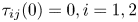 $\tau _{ij}(0) = 0, i=1,2$. The dimensionless steady shear viscosity
  $\mu _s/\mu _0 = \beta + \tau _{12}/\dot {\gamma }$ as a function of
  $Wi$ is reported in figure 3. As expected, both models exhibit a shear-thinning behaviour: in particular, for
  $L^2=\infty$ the model tends to a plateau at both low (
 $Wi \lesssim 0.1$) and high (
 $Wi \gtrsim 10$) Weissenberg numbers, while for
  $L^2=100$ the steady shear viscosity reaches a plateau at low
  $Wi$ but it decreases monotonically at high
  $Wi$. Note that the shear-thinning effect is controlled by
  $Bi$, which modifies the plateau value at low
  $Wi$.
$Wi$.

Figure 3. Steady shear viscosity for  $\beta =0$ and (a)
  $L^2=\infty$ (Oldroyd-B model); (b)
  $L^2=100$ (FENE-P model).
3. Results
3.1. Laminar flow
Our first analysis considers the laminar flow of an EVP fluid. All laminar cases are fixed at  $\beta =0.9$,
  $Re=2800$ and
  $L^2=3600$, while the Weissenberg and the Bingham numbers are varied in the range of
  $0.01 \le Wi \le 16$ and
  $0.1 \le Bi \le 100$, respectively. Note that the domain size in the homogeneous directions was kept very small to avoid the development of a turbulent flow and that no perturbations were added to the zero initial condition.
First, we consider the combined effects of the Bingham and the Weissenberg numbers on the frictional resistance of the flow quantified by the Fanning friction factor  $f$, defined as
  $2 \tau _w/\rho U_b^2$ with
  $\tau _w$ the total wall shear stress including both the viscous and EVP contributions. Figure 4(a) shows the Fanning friction factor
  $f$ as a function of the Weissenberg number for various Bingham numbers. In particular, the cyan, brown, purple and green lines are used for
  $Bi=0.1$,
  $2.8$,
  $11.2$ and
  $100$, respectively. The friction factor
  $f$ decreases nearly linearly with
  $Wi$ (in log scale). However, at
  $Bi=0.1$ the factor
  $f$ is constant, which is consistent with the viscoelastic flows in the laminar regime. Results clearly show that the elastic effects become more prominent with
  $Bi$, leading to a steeper decay with
  $Wi$.
$Wi$.

Figure 4. Fanning factor as a function of (a) the Weissenberg number for  $Bi=0.1,2.8,11.2$ and
  $100$ and (b) the Bingham number for
  $Wi=0.01,0.1,2$ and
  $16$.
$16$.
Next, we consider the reverse case, where we study the effects of Bingham number at a fixed  $Wi$, as shown in figure 4(b). We find that
  $f$ increases nonlinearly with the Bingham number
  $Bi$, and that the dependency on
  $Bi$ decreases with the Weissenberg number
  $Wi$. The increase of
  $f$ can be explained by subtle changes in the mean streamwise velocity profile. The non-dimensional streamwise velocity profile u/U b is shown in figure 5(a) at
  $Wi=0.01$ and
  $Bi=0.1,2.8,11.2,100$ as a function of the wall-normal distance
  $y/h$. It can be seen that the solid plug in the middle of the channel increases with the Bingham number. The plug moves with a uniform velocity, and its velocity decreases with
  $Bi$ due to mass conservation, leading to an increase in the wall shear stress.

Figure 5. Mean streamwise velocity profile  $u$ as a function of (a) the Bingham number for
  $Bi=0.1,2.8,11.2$ and 100 at
  $Wi=0.01$ and (b) the Weissenberg number for
  $Wi=0.01,0.1,2$ and
  $16$ at
  $Bi=22.4$.
The variations of the non-dimensional mean velocity profile  $u/U_b$ at
  $Bi=22.4$ with the Weissenberg number, see figure 5(b), demonstrate that the solid plug in the middle of the channel decreases with
  $Wi$. Indeed, the total stress magnitude in a channel flow increases with elasticity, leading to earlier yielding (Chaparian & Tammisola Reference Chaparian and Tammisola2019). To further quantify these observations, the volume of the solid region is shown in figure 6 for various combinations of
  $Wi$ and
  $Bi$. The results are consistent with the observations in figure 4, since the solid volume
  $Vol_s$ is proportional to the friction factor
  $f$.
$f$.

Figure 6. Percentage of the unyielded volume  $Vol_s$ as a function of (a) the Weissenberg number for
  $Bi=0.1,2.8,11.2$ and
  $100$ and (b) the Bingham number for
  $Wi=0.01,0.1,2$ and
  $16$.
$16$.
3.2. Turbulent flow
We examine turbulent channel flows of an EVP fluid, together with the baseline Newtonian ( $Bi=0$ and
  $Wi \approx 0$), viscoelastic (
 $Bi=0$) and almost viscoplastic (
 $Wi \approx 0$) cases. All simulations have been performed until statistically steady state (at least 500 non-dimensional units). Hence, in the turbulent flow cases, the turbulence is always fully developed. However, for some parameter values the flow is not turbulent, because it has laminarised by increasing elasticity or plasticity.
The flow rate is constant in all simulations, so that the flow Reynolds number based on the bulk velocity is fixed, i.e.  $Re=\rho U_b h/\mu _0=2800$, where the bulk velocity
  $U_b$ is the average value of the mean velocity computed across the whole domain and
  $\mu _0$ is the total zero-shear viscosity. In the turbulent regime, this bulk Reynolds number corresponds to a nominal friction Reynolds number
  $Re_\tau =\rho u_\tau h/ \mu _0=180$ for a Newtonian fluid,
  $u_\tau$ being the friction velocity. A wide range of elasticity and plasticity is investigated: the Weissenberg number
  $Wi=\lambda U_b/h$ is varied in the range
  $0\le Wi \le 16$ to study the role of fluid elasticity, while the Bingham number
  $Bi=\tau _0 h/ \mu _0 U_b$ is varied between
  $0$ and
  $22.4$. The viscosity ratio and the extensibility parameter are fixed to
  $\beta =\mu _f / \mu _0 =0.9$ and
  $L^2=3600$.
The viscous units used above are indicated by the superscript  $^+$, and are built using the friction velocity
  $u_\tau$ as the velocity scale and the viscous length
  $\delta _\nu = \nu / u_\tau$ as the length scale. Here, we define the friction velocity as
 \begin{equation} u_\tau = \sqrt{ \left. \left( \frac{1}{Re_b} \frac{\textrm{d} \bar{u}}{\textrm{d} y} + \bar{\tau}_{12} \right) \right\vert_{y=0}}, \end{equation}
where we have taken into account also the EVP shear stress at the wall. Note that the actual value of the friction velocity in our simulations is computed from the friction coefficient, obtained with the driving streamwise pressure gradient, rather than from its definition.
We first discuss the qualitative flow characteristics for various combinations of  $Wi$ and
  $Bi$. A qualitative overview of the resulting flow regimes as functions of
  $Wi$ and
  $Bi$ is presented in figure 7.

Figure 7. Combined effects of elasticity and plasticity. A flow regime map is shown by symbols:  $\square$ – turbulent,
  $\blacksquare$ – laminar. Colour scale shows drag reduction compared with the Newtonian case. (a) Colour scale:
  $DR =[1-(Re_\tau /Re_{\tau ,Wi=0})^2] \times 100\,\%$ spanning
  $\pm 65$ from red (drag reduction) to violet (drag increase). (b) Colour scale:
  $DR_2 =[1-f_{EVP} /f_{N}] \times 100\,\%$ where
  $f_{EVP}$ and
  $f_N$ denote skin friction for EVP and Newtonian cases, respectively.
The empty and filled symbols in figure 7 represent turbulent and laminar regimes, respectively. As expected, the flow becomes laminar and steady with an increasing Bingham number. The critical  $Bi_c$ can be defined as the lowest value of
  $Bi$ where laminarisation occurs, at each
  $Wi$. At
  $Wi=0.01$, the flow is near viscoplastic and fully laminarises at the relatively low critical
  $Bi_{c}=2.8$ (Rosti et al. Reference Rosti, Izbassarov, Tammisola, Hormozi and Brandt2018c). (Note that results for viscoplastic cases used in this work are taken from our previous work Rosti et al. (Reference Rosti, Izbassarov, Tammisola, Hormozi and Brandt2018c).) Laminarisation of the viscoplastic flow with increasing Bingham number is closely related to the increase of the core unyielded region which grows from the centreline towards to the walls, and damps out turbulent fluctuations in the core. As described in Rosti et al. (Reference Rosti, Izbassarov, Tammisola, Hormozi and Brandt2018c), the near-wall streaks were intensified and became more coherent. The low-speed streaks, usually associated with positive wall-normal fluctuations, reach higher wall-normal distances than the high-speed streaks, thus inducing the flow to yield at higher wall-normal distances if the local stress reaches the yield-stress threshold. Indeed, the unyielded regions preferentially form above high-speed streaks. Overall, the flow becomes more and more correlated in the streamwise direction when increasing the Bingham number, with high levels of flow anisotropy close to the wall, similarly to what observed in other drag-reducing flows. Differently from the other flows, however, both the streamwise and spanwise correlations grow with the Bingham number also away from the wall, due to the growth of the unyielded region.
As the flow becomes more elastic, the critical  $Bi_{c}$ shows a non-monotonic behaviour; it first increases with
  $Wi$, then decreases. The reason for this non-monotonic behaviour is attributed to the fact that the coherent structures are highly influenced by the relative width of the plug compared with the yielded regions around it, as will be described later.
The colours in figure 7 represent a measure of drag reduction compared with a Newtonian fluid. Panel (a) shows  $DR =[1-(Re_\tau /Re_{\tau ,Wi=0})^2] \times 100\,\%$. For flows in the turbulent regime,
  $DR$ increases with
  $Bi$ for all
  $Wi$ studied in this work. In the laminar regime, however, at low
  $Wi=0.01$, the
  $DR$ changes sign, showing drag increase, whereas for higher
  $Wi\ge 2$ values, the
  $DR$ only slightly decreases with
  $Bi$. This is consistent with the results for the Fanning factor shown in figure 8. It is well known that a finite viscoelasticity reduces drag compared with a Newtonian flow, and this has been exploited in many previous studies and in the industry. The figure seems to show that a combination of finite
  $Wi$ and
  $Bi$ results in a much greater drag reduction than a finite
  $Wi$ alone. However, a closer inspection shows that the very high drag reduction
  $DR>70\,\%$ occurs when the flow laminarises, because we compare with the drag in the Newtonian flow in the turbulent regime. We wanted to eliminate the effect of laminarisation on drag reduction, and also try to exclude the effects of shear thinning. Therefore, in (b), we show another measure of drag reduction which excludes the influence of shear thinning (Housiadas & Beris Reference Housiadas and Beris2003):
  $DR_2 =[1-f_{EVP} /f_{N}] \times 100\,\%$, where
  $f_{EVP}$ and
  $f_N$ denote skin friction for EVP and Newtonian cases, respectively. Following Dean (Reference Dean1978)
 \begin{equation} f_N = \begin{cases}
12/Re_w & {laminar}\\ 0.073 Re_w^{{-}0.25} & {turbulent},
\end{cases} \end{equation}
\begin{equation} f_N = \begin{cases}
12/Re_w & {laminar}\\ 0.073 Re_w^{{-}0.25} & {turbulent},
\end{cases} \end{equation}
where  $Re_w=\rho U 2h/\mu _w$ and
  $\mu _w=\tau _w/\dot {\gamma _w}$, and subscript
  $w$ denotes wall quantities. Using
  $DR_2$ as a measure, the highest drag reduction is achieved either at high
  $Wi$, or in EVP flow when
  $Wi$ and
  $Bi$ are both moderate, in the same region where laminarisation is delayed to higher
  $Bi$. In general, the drag-reduction values remain very similar for these two measures in the turbulent regime, indicating that shear thinning has no major influence on drag reduction at the studied parameter values. Despite this, the viscosity profiles (figure 8) show shear thinning for VE, EVP and VP cases. Apparently, plasticity plays a strong role on shear thinning, as both VP and EVP show stronger shear thinning. For the EVP case at
  $Wi=4$ and
  $Bi=5.6$, we are approaching results of VP at
  $Bi=1.4$, thus elasticity seems to decrease shear thinning.

Figure 8. The shear effective viscosity  $\mu _e$ for (a) VE, (b) VP and (c) EVP cases. (a) VE case: the green, magenta, black and blue colours are used for
  $Wi = 2$, 4, 8 and 16. (b) VP case: the red, orange, cyan and violet colours are used for
  $Bi = 0$, 0.28, 0.7 and 1.4, respectively (c) EVP case is at fixed
  $Wi=4$ and the green, red and black colours are used for
  $Bi = 0$, 2.8 and 5.6, respectively.
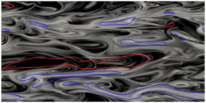
The main area responsible for the non-monotonic trends is the unyielded region of the flow. The unyielded regions show a non-trivial and complex trend with  $Bi$ and
  $Wi$, with significant differences also between the laminar and turbulent regimes. In order to better understand the flow, we start by showing visualisations of the instantaneous distributions of the yielded and unyielded regions in figure 9. In particular, the figure shows instantaneous cross-stream planes (
 $x$–
$x$– $y$ plane) where the unyielded regions are coloured in brown; in the yielded regions we report colour contours of the spanwise vorticity,
  $\omega _z$. At
  $Bi=0$ and
  $Wi \approx 0$ we recognise the classic vorticity field of turbulent channel flows, with high vorticity levels at the walls, and the footprints of the classical turbulent streaky structures. As
  $Wi$ increases, the flow becomes smoother, the flow structures seem to be more elongated and the streamwise coherency of the flow increases, as is typical of drag-reducing flows.

Figure 9. Contours of the instantaneous spanwise vorticity  $-\omega _z$ in a
  $x$–
$x$– $y$ plane As a function of the Bingham and Weissenberg numbers. Colour scale ranges from
  $-3U_b/h$ (blue) to
  $3U_b/h$ (red). The brown areas represent the instantaneous regions where the flow is not yielded.
Note that, although the turbulence activity is reducing with  $Wi$, the purely viscoelastic flow does not laminarise. On the other hand, for every
  $Wi$, the flow returns to laminar for a sufficiently high Bingham number (
 $Bi > Bi_c$). In particular, we observe that as
  $Bi$ increases, the amount of fluid which is unyielded grows, eventually forming a fully connected plug spanning the whole streamwise and spanwise lengths, thus leading to the decay of turbulence and the return to a fully laminar regime. However, at intermediate
  $Wi$, we observe that a higher
  $Bi_c$ is required to laminarise the flow than at low or high
  $Wi$. At intermediate
  $Wi$, the equilibrium solutions indicate that the unyielded region is narrower than in the viscoplastic flow (Chaparian & Tammisola Reference Chaparian and Tammisola2019), and we propose that this allows instabilities to be sustained in the yielded regions. In the present simulation at intermediate
  $Wi$, a plug was formed initially and the flow seemed to laminarise, but soon a large-scale roll-up motion developed at the edges of the unyielded region, recreating the unsteadiness and turbulence. On the other hand, at higher values (
 $Wi>4$) this effect does not occur thus leading to lower
  $Bi_c$. This phenomenon could be attributed to the fact that the unyielded region becomes too thin to create any instability. Moreover, the yielded region becomes smoother at high
  $Wi$ enhancing laminarisation.
It is not obvious what drives the instability leading to the roll-up motion, because the laminar flow profile is not inflectional. A sharp viscosity contrast can lead instabilities in channel and shear flows. The unyielded region could play a similar role as a high-viscosity fluid in the centre of the channel, a configuration which can be unstable at high Reynolds numbers (Hooper & Boyd Reference Hooper and Boyd1987; Govindarajan & Sahu Reference Govindarajan and Sahu2013). On the other hand, a channel flow of Bingham fluid is known to be linearly stable at all Reynolds numbers. Although the linear stability of EVP flow has not been studied, the transition that we observe could be subcritical, like for Bingham fluids. However, the roll-up structure we observe does not resemble the optimal non-modal instabilities in Bingham fluid: streamwise-travelling waves (Nouar et al. Reference Nouar, Kabouya, Dusek and Mamou2007) or oblique waves (Nouar & Bottaro Reference Nouar and Bottaro2010).
For laminar flows ( $Bi>Bi_c$), a further increase of
  $Bi$ leads to a growth of the unyielded region, which induces an increase of the wall shear stress and a consequent drag increase, as previously observed in figure 8. This is different from observations in the turbulent regime, where the drag reduces with both
  $Wi$ and
  $Bi$ (Rosti et al. Reference Rosti, Izbassarov, Tammisola, Hormozi and Brandt2018c).
3.3. Flow statistics
Here, we discuss the turbulent statistics for EVP flows. To facilitate comparisons, we provide results for the two limiting cases: near-viscoplastic and viscoelastic flows, and then compare these with the flows with finite elasticity and plasticity. The near-viscoplastic flow was presented in our earlier work (Rosti et al. Reference Rosti, Izbassarov, Tammisola, Hormozi and Brandt2018c), and was computed using the Saramito model at  $Wi=0.01$,
  $\beta =0.95$, and varying
  $Bi$. The viscoelastic flow is computed at varied Weissenberg number
  $0 \le Wi \le 16$ and fixed Bingham number
  $Bi=0$, and the FENE-P model parameters are
  $\beta =0.9$ and
  $L^2=3600$, unless indicated otherwise.
We first discuss the mean streamwise velocity profiles in relation to drag reduction shown in figure 7. In figure 10, the velocity profiles are shown in wall units. The profiles for viscoplastic flow in figure 10(a) are similar to the Newtonian case for  $Bi<1.4$. For
  $Bi=1.4$, the difference becomes more significant with zero-shear region at the centreline. At
  $Bi=2.8$, the flow becomes laminar with a large zero-shear region, leading to drag increase as observed in figure 7. We can observe that the flow remains unyielded mostly in the logarithmic and outer layer, while it is always yielded in the viscous sublayer.

Figure 10. Mean streamwise velocity profile  $\bar {u}$ as a function of the wall-normal distance
  $y$ in wall units. (a) Near-viscoplastic flow (
 $Wi=0.01$). (b) Viscoelastic flow (
 $Bi=0$). The dashed line and symbols in the figure correspond to the Virk curve at maximum drag reduction (Virk Reference Virk1975) and the results of Kim, Moin & Moser (Reference Kim, Moin and Moser1987), respectively.

Figure 11. EVP flow: (a) drag reduction as a function of  $Bi$ and (b) mean streamwise velocity profile
  $\bar {u}$ as a function of the wall-normal distance
  $y$ in wall units. The Weissenberg number
  $Wi$ and the extensibility parameter
  $L^2$ are fixed and equal to
  $4$ and
  $3600$, respectively (FENE-P model).

Figure 12. Wall-normal profiles of components of the Reynolds stress tensor, normalised with  $u_\tau ^2$. The first column shows
  $u'u'$, the second column
  $v'v'$. (a,b) VE flow at various
  $Wi$ and fixed
  $Bi=0$. (c,d) VP flow at various
  $Bi$ and fixed
  $Wi=0.01$. (e,f) EVP flow at various
  $Bi$ and fixed
  $Wi=4$. The extensibility parameter
  $L^2$ is fixed and equal to
  $3600$. The
  $\bullet$, blue symbols indicate the direct numerical simulation (DNS) data of Kim et al. (Reference Kim, Moin and Moser1987).

Figure 13. Wall-normal profiles of components of the Reynolds stress tensor, normalised with  $u_\tau ^2$. The first column shows
  $w'w'$, the second column
  $u'v'$. (a,b) VE flow at various
  $Wi$ and fixed
  $Bi=0$. (c,d) VP flow at various
  $Bi$ and fixed
  $Wi=0.01$. (e,f) EVP flow at various
  $Bi$ and fixed
  $Wi=4$. The extensibility parameter
  $L^2$ is fixed and equal to
  $3600$. The
  $\bullet$, blue symbols indicate the DNS data of Kim et al. (Reference Kim, Moin and Moser1987).
For viscoelastic flows,  $DR \%$ increases monotonically with
  $Wi$ in the range of
  $Wi={O}(1)$ and start to saturate at
  $Wi>10$. The maximum drag reduction is close to
  $40\,\%$ at
  $Wi=16$. Figure 10(b) shows the mean streamwise velocity profiles in wall units. It can be seen that increasing
  $Wi$ the velocity profiles collapse in the viscous sublayer, however, shift upward in the buffer region (thickening of the buffer layer) and are parallel to the Newtonian profile. Note that we do not reach Virk's maximum drag-reduction (MDR) asymptote (Virk Reference Virk1975), which is out of scope of the present study. The shift in the velocity profile is consistent with results in the literature (Xi & Graham Reference Xi and Graham2010; Shahmardi et al. Reference Shahmardi, Zade, Ardekani, Poole, Lundell, Rosti and Brandt2019).
We next consider the EVP flow. The drag-reduction values and the corresponding mean streamwise velocity profiles for  $Wi=4, \beta =0.9, L^2=3600$ and
  $Bi=0$, 2.8, 5.6, 11.2 and
  $22.4$ are shown in figure 11. Similarly to the viscoplastic flow, the
  $DR \%$ increases with
  $Bi$ in the turbulent regime. Unlike pure viscoelastic case, plasticity enhances the
  $DR$ going from low-drag reduction (LDR,
  $DR\lesssim 40$) at
  $0 \le Bi < 5.6$ to high drag-reduction (HDR,
  ${40< DR\lesssim 60}$) at
  $Bi=5.6$. Moreover, the laminar regime delays to larger
  $Bi>5.6$, which may be attributed to the dramatic effects due to the polymer dynamics. Unlike the viscoplastic case,
  $DR \%$ only slightly decreases in the laminar case as shown also earlier in figure 7. The change of mean streamwise velocity profile with
  $Bi$ is more significant than in figure 10(a) and more similar to figure 10(b) for
  $Bi\le 5.6$, i.e. the velocity profile collapse in the viscous sublayer, and shift upward in the buffer and log-law layer approaching Virk's asymptote. In contrast, for
  $Bi>5.6$ the flow fully laminarises and becomes similar to the case in figure 10(a), with the zero-shear region at the centreline.
Next, we analyse the wall-normal distribution of the Reynolds stress components  $\overline {u'u'}$ and
  $\overline {v'v'}$, shown in figure 12 together with the Newtonian case by Kim et al. (Reference Kim, Moin and Moser1987) (blue symbol). The profiles are normalised with
  $u_\tau ^2$. The results for the viscoelastic case (a,b) show that the
  $\overline {u'u'}$ increases while
  $\overline {v'v'}$ decreases with
  $Wi$. In general, the shape of the profiles is similar to the corresponding Newtonian one, but the magnitude changes with
  $Wi$. Moreover, all the peaks move towards the channel centre, in agreement with the thickening of the buffer layer observed in the mean velocity profile. A similar behaviour has been noticed in the literature for drag-reducing turbulent viscoelastic flows (White & Mungal Reference White and Mungal2008; Dallas, Vassilicos & Hewitt Reference Dallas, Vassilicos and Hewitt2010). The VP case (
 $Wi=0.01$) is depicted in (c,d) to examine the effects of the Bingham number in the range
  $0\le Bi \le 2.8$. We clearly observe that the peak of the streamwise component
  $\overline {u'u'}$ increases with
  $Bi$, while it decreases for
  $\overline {v'v'}$. A similar trend is observed for the EVP case (
 $Wi=4$) as depicted in (e,f).
Although the overall trends are similar, the combined effects of elasticity and plasticity in the EVP flows result in larger deviations from the Newtonian flow than for the two limiting cases, particularly for the peak in the  $\overline {u'u'}$ profile. It is also interesting to note that in the EVP flow the peak moves non-monotonically, unlike in the VE and VP cases: it first moves away from the wall as
  $Bi$ increases (
 $Bi\le 5.6$), and then moves slightly back towards the wall. The stress components
  $\overline {u'v'}$ and
  $\overline {w'w'}$ show similar trends as
  $\overline {v'v'}$, and are shown in figure 13 for completeness.
Figure 14 shows  $P_s$, the probability of the fluid being unyielded in a given vertical position, and
  $Vol_s$, the percentage of the volume that was unyielded on average, for VP (
 $Wi=0.01$) and EVP (
 $Wi=4$ and 8) cases. The probability
  $P_s$ is displayed against the wall-normal distance
  $y$, whereas the volume percentage is depicted in the legend. The probability
  $P_s$ ranges from 0 (always fluid) to 1 (always elastic solid).

Figure 14. Probability of the fluid being unyielded  $P_s$ in: (a) VP flow at
  $Wi=0.01$ and EVP cases at (b)
  $Wi=4$ and (c)
  $Wi=8$. The percentage of the unyielded volume
  $Vol_s$ is presented in the legends. For the (a) VP case, the red, orange, cyan, violet and green colours are used for
  $Bi=0$,
  $0.28$,
  $0.7$,
  $1.4$ and
  $2.8$, respectively. For the (b,c) EVP cases, green, red, black and orange colours are used for
  $Bi=0$,
  $2.8,5.6$ and
  $11.2$, respectively. The extensibility parameter for the EVP cases is
  $L^2=3600$.
For the laminar case, as expected,  $P_s$ sharply changes along the interface between the unyielded and yielded region. For turbulent cases, the probability
  $P_s$ increases smoothly across the channel with a maximum in the vicinity of the centreline and a minimum near the wall. This happens due to the time-dependent nature of the turbulent flow.
For the VP case,  $P_s$ and
  $Vol_s$ increase with
  $Bi$, reaching the maximum (
 $Vol_s=54\,\%$) at
  $Bi=2.8$, when the flow is fully laminar. The volume of the unyielded region further increases when
  $Bi$ increases in the laminar regime, as illustrated in figure 5(a). Let us now consider the EVP cases. A careful inspection of figure 14 reveals that the unyielded volume
  $Vol_s$ is smaller in EVP flows than in VP flows, in both laminar and turbulent states. Also,
  $Vol_s$ further decreases as
  $Wi$ increases, from
  $30\,\%$ at
  $Wi=4$ to
  $26\,\%$ at
  $Wi=8$, as seen in figure 14(b,c). The reason is that the elastic stress in channel flows increases with
  $Wi$, resulting in a smaller unyielded volume. Moreover, the
  $Vol_s$ increases monotonically with
  $Bi$ also for the EVP case, as long as
  $Bi< Bi_c$. However, when the flow laminarises (
 $Bi \ge Bi_c$),
  $Vol_s$ decreases owing to a narrow plug region. An explanation to the decrease can be found by comparing the laminar and turbulent mean flow profiles. In laminar VE channel flows, the elastic stress is known to be proportional to both the local shear and
  $Wi$, and therefore, the elastic stress forms the largest part of the total stress at moderate
  $Wi$. In laminar flows, the shear is finite almost everywhere across the channel. In turbulent flows, however, the mean flow shear is small in the central region, and hence the elastic stresses are smaller on average, with the Reynolds stresses becoming more important in yielding the material.
We now present the statistics of the polymer conformation tensor for VE, VP and EVP cases. The mean profiles of the polymer stretching  $\sqrt {\textrm {Tr}(\bar {C})}/L$ are shown in figure 15(a) for the VE case at
  $Wi=2,4,8$ and 16, where the dashed line in the figure indicates the case of coiled polymers (conformation tensor equal to identity). As expected, the polymer stretching increases monotonically with the Weissenberg number
  $Wi$. The mean polymer stretching first increases with maximum in the vicinity of the wall, then decreases with minimum at the centre. The observed near-wall peak is mostly due to the interaction between polymers and near-wall vortices (Xi & Graham Reference Xi and Graham2010; Dubief, Terrapon & Soria Reference Dubief, Terrapon and Soria2013). Viscoelastic effects become more prominent throughout the domain when increasing
  $Wi$ and the peak values move away from the wall.
The mean polymer extension for the VP cases at  $0\le Bi \le 2.8$ is shown in figure 15(b). For
  $Bi \lesssim 2$, corresponding to the turbulent regime, the stress profile is nearly constant except in the near-wall region where it is maximum. Note that, for the laminar case, the stress monotonically decreases along the wall-normal direction. Finally, the results pertaining the EVP flows at
  $0\le Bi \le 11.2$ and
  $Wi=$4
  $\&$ 8 are presented in figure 15(c,d). For the turbulent EVP cases (
 $Bi<11.2$), the stress profiles are qualitatively similar to the VE ones. The maximum values are in the vicinity of the wall and the minimum at the centreline (
 $y=h$). Moreover, the minimum values increase with
  $Bi$ while peaks are not sensitive to
  $Bi$ at
  $Bi< Bi_c$. For the laminar flows, the profile is qualitatively similar to the viscoplastic one, with maximum and minimum values at the wall and centreline, respectively.

Figure 15. Mean polymer extension in: (a) VE ( $Bi=0$), (b) VP (
 $Wi=0.01$), EVP for (c)
  $Wi=4$ and (d)
  $Wi=8$. The undeformed polymer stretching (
 $\sqrt {\textrm {Tr}({{I}})}/L$ and
  $\sqrt {\textrm {Tr}({{I}})}$) is represented by the black dashed line. The extensibility parameter is
  $L^2=3600$.

Figure 16. VE case: wall-normal profiles of (a) the turbulent kinetic energy  $\mathcal {K}=( u'^2 + v'^2 + w'^2 )/2$ and of (b) the turbulent production
  $\mathcal {P}=-\overline {\rho u'v'} \,\textrm {d}\bar {u}/{\textrm {d} y}$, (c) the turbulent dissipation
  $\varepsilon =\mu \overline {\partial u'_i/\partial x_j \partial u'_i/\partial x_j}$ and (d) average contributions to the energy balance from
  $\mathcal {P}, \varepsilon$ and dissipation due to the polymers
  $\varPi =\overline {\partial u'_i/\partial x_j \tau '_{ij} }$, all normalised with the friction velocity
  $u^3_\tau$. The symbols in the figure correspond to results of Kim et al. (Reference Kim, Moin and Moser1987) for the Newtonian case.
3.4. Energy and stress balance
To further characterise the flow, we study the energy and shear stress budget for the viscoelastic and EVP cases. We first consider how the energy stress budgets evolve with Weissenberg number, at zero Bingham number.
An overall view of the velocity fluctuations is obtained from the turbulent kinetic energy  $\mathcal {K}=( u'^2 + v'^2 + w'^2 )/2$, normalised with
  $u^2_\tau$ (figure 16a). Following Dallas et al. (Reference Dallas, Vassilicos and Hewitt2010), the budget of turbulent kinetic energy integrated over the whole domain can be written as follows:
 \begin{equation} \int\limits_{\mathcal{V}} \mathcal{P}\,\textrm{d}\mathcal{V}= \int\limits_\mathcal{V} \varepsilon \,\textrm{d}\mathcal{V}+\int\limits_\mathcal{V} \varPi \,\textrm{d}\mathcal{V}, \end{equation}
where  $\mathcal {V}$ is the volume of the domain,
  $\mathcal {P}=-\overline {\rho u'v'} \,\textrm {d}\bar {u}/{\textrm {d} y}$ is the turbulent production,
  $\varepsilon =\mu \overline {\partial u'_i/\partial x_j \partial u'_i/\partial x_j}$ is the turbulent dissipation and
  $\varPi =\overline {\partial u'_i/\partial x_j \tau '_{ij} }$ is the dissipation due to the polymers.
The turbulent kinetic energy increases with  $Wi$, and its profile is similar to the streamwise velocity fluctuation in figure 12(a), as the streamwise velocity is of larger magnitude than the other velocity components. On the other hand, the turbulent production by the Reynolds shear stress
  $\mathcal {P}=-\overline {u'v'} \,\textrm {d}\bar {u}/{\textrm {d} y}$ is continuously reduced when increasing
  $Wi$. The peak values occur in the buffer layer, moving towards the channel centre with increased
  $DR$ consisted with thickening of the buffer layer. We also computed the turbulent dissipation
  $\varepsilon =\mu \overline {\partial u'_i/\partial x_j \partial u'_i/\partial x_j}$ of the fluctuating velocity field
  $u_i'$. The dissipation
  $\varepsilon$ also attenuates with
  $Wi$, while the profile maintains its shape with maximum value at the wall and minimum at the centreline. Volume-averaged quantities of
  $\int \mathcal {P}\, {\textrm {d} y}, \int \varepsilon \,{\textrm {d} y}$ and dissipation due to polymers
  $\int \varPi \,{\textrm {d} y}$ are shown in figure 16(d). It can be seen that the average turbulent production and viscous dissipation decrease with
  $Wi$, while the polymeric dissipation increases with
  $Wi$. The decrease in
  $\mathcal {P}$ and
  $\varepsilon$ with
  $Wi$ is consistent with the observed drag reduction. Note that
  $\varPi$ first increases with
  $Wi$, but slightly decreases at
  $Wi=16$, which could be due to the fact that we are approaching the HDR regime. Dallas et al. (Reference Dallas, Vassilicos and Hewitt2010) observed a similar non-monotonic trend with
  $Wi$ for
  $\varPi$ i.e. the polymeric dissipation increases in LDR while it decreases in HDR and MDR. Overall, our viscoelastic results are in agreement with the literature for turbulent flow with polymer additives (Warholic, Massah & Hanratty Reference Warholic, Massah and Hanratty1999; Dallas et al. Reference Dallas, Vassilicos and Hewitt2010; Xi & Graham Reference Xi and Graham2010).
Next, we show the mean viscous ( $\bar {\tau }_{V}$) and viscoelastic stress (
 $\bar {\tau }_{E}$) profiles as a function of the Weissenberg number, see figure 17. The viscous stress profiles coincide close to the wall and in the vicinity of the channel core but increase slightly in the buffer layer. The viscoelastic stress profile has a peak in the vicinity of the wall and minimum in the centre. The
  $\bar {\tau }_{E}$ changes non-monotonically, it first increases reaching maximum in the buffer layer and then decreases reaching a minimum at the centreline. With increase in
  $Wi$ the peak moves towards the core region.
To gain further understanding, the shear stress budget is shown in figure 18 for the VE cases with  $Wi=2$ and
  $Wi=16$, normalised with the corresponding wall stress. The total shear stress
  $\bar {\tau }_{T}$ can be written as
  $\bar {\tau }_{T}=\bar {\tau }_{V}+\bar {\tau }_{E}+\bar {\tau }_{R}=(1-y/h)\tau _w$ where the viscous stress
  $\bar {\tau }_{V}=\mu \,\textrm {d}\bar {u}/{\textrm {d} y}$, the Reynolds stress
  $\bar {\tau }_{R}=-\rho \overline {u'v'}$ and viscoelastic stress
  $\bar {\tau }_{E}$ tensor. Note that, unlike the Newtonian case, the total wall shear stress is sum of the viscous and viscoelastic contributions. For
  $Wi=2$, the behaviour is similar to the Newtonian case with the viscous stress dominating close to the wall and the Reynolds stress in the core. The viscoelastic effects become more pronounced at
  $Wi=16$, in that the viscous and viscoelastic stresses increase, while the Reynolds stresses diminish.

Figure 17. VE case: shear component of the mean (a) viscous stress  $\bar {\tau }_{V}$ and (b) viscoelastic stress tensor
  $\bar {\tau }_{E}$ as a function of the wall-normal distance
  $y$. The extensibility parameter
  $L^2$ is fixed and equal to
  $3600$.

Figure 18. VE case: normalised shear stress balance across the channel, for (a)  $Wi=2$ and (b)
  $Wi=16$. The total shear stress varies linearly across the channel height.

Figure 19. EVP case: wall-normal profiles of (a) the turbulent kinetic energy 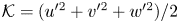 $\mathcal {K}=( u'^2 + v'^2 + w'^2 )/2$ and of (b) the turbulent production
  $\mathcal {P}=-\overline {\rho u'v'} \,\textrm {d}\bar {u}/{\textrm {d}y}$, (c) the turbulent dissipation
 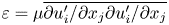 $\varepsilon =\mu \overline {\partial u'_i/\partial x_j \partial u'_i/\partial x_j}$ and (d) average contributions to the energy balance due to
  $\mathcal {P}, \varepsilon$ and dissipation due to fluctuation of the EVP stresses
 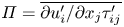 $\varPi = \overline {\partial u'_i/\partial x_j \tau '_{ij} }$, all normalised with the friction velocity
  $u_\tau$. The Weissenberg number
  $Wi$ and the extensibility parameter
  $L^2$ are fixed and equal to
  $4$ and
  $3600$, respectively (FENE-P model). The symbols in the figure correspond to results of Kim et al. (Reference Kim, Moin and Moser1987) for the Newtonian case.
Finally, we perform the same energy and momentum budget analysis to consider the combined effects of elasticity and plasticity. The energy budget is shown in figure 19 at fixed Weissenberg number  $Wi=4$, while varying the Bingham number in the range
  $0 \le Bi \le 11.2$. Qualitatively, the effect of Bingham number on the energy budget is similar to the viscoplastic case in Rosti et al. (Reference Rosti, Izbassarov, Tammisola, Hormozi and Brandt2018a), the peak of
  $\mathcal {K}$ increases with
  $Bi$, while the peak values for
  $\mathcal {P}$ and
  $\varepsilon$ decrease. The volume-averaged viscous dissipation decreases, while EVP dissipation increases with
  $Bi$. Surprisingly, however, the turbulent production slightly increases with
  $Bi$ at this finite Weissenberg number, in contrast with the viscoplastic flow. The shear components of the mean viscous and EVP stress tensors are shown in figure 20. In viscoplastic flows, we observed that the shear component of the EVP stress tensor increased everywhere across the channel. In the combined case, however, (figure 20b) its value at the wall remains constant in the turbulent regime. In the laminar regime, as expected, the shear component changes linearly in the liquid region and is zero in the solid region. The EVP stress continuously increases with
  $Bi$ towards the centre of the channel. Finally, we report in figure 21 the shear stress budget for the cases with
  $Bi=0$ and
  $Bi=5.6$, normalised with the corresponding wall stress. With increasing
  $Bi$, the EVP and viscous stresses grow more across the channel, further reducing the Reynolds stresses, and hence the combined case deviates even more from the Newtonian flow than the viscoelastic case does.

Figure 20. EVP case: shear component of the mean (a) viscous stress  $\bar {\tau }_{V}$ and (b) EVP stress tensor
  $\bar {\tau }_{E}$ as a function of the wall-normal distance
  $y$. The Weissenberg number
  $Wi$ and the extensibility parameter
  $L^2$ are fixed and equal to
  $4$ and
  $3600$, respectively (FENE-P model).

Figure 21. EVP case: normalised shear stress balance across the channel, for (a)  $Bi=0$ and (b)
  $Bi=5.6$. The total shear stress varies linearly across the channel height. The Weissenberg number
  $Wi$ and the extensibility parameter
  $L^2$ are fixed and equal to
  $4$ and
  $3600$, respectively (FENE-P model).

Figure 22. Time series for hibernation phenomenon. Left column: the  $Re_{\tau}$ evolution in time; right column: mean streamwise velocity at time instants i–v defined in the left column, for VE flow (a,b), VP flow (c,d) and EVP flow (e,f). The parameters are:
  $Wi=16$ and
  $Bi=0$ for VE flow,
  $Wi=8$ and
  $Bi=2.8$ for EVP flow and
  $Wi=0.01$ and
  $Bi=1.4$ for VP flow.
3.5. Intermittent dynamics
Finally, we compare the intermittent dynamics for purely viscoelastic, viscoplastic and EVP cases. Previously, Xi & Graham (Reference Xi and Graham2010, Reference Xi and Graham2012b) observed two distinct time intervals, denoted as hibernating and active, for viscoelastic turbulent flow in minimal channel geometry. During the hibernating intervals, drag reduction is high and turbulence is partly attenuated, whereas the active intervals represent active turbulence similar to the Newtonian turbulent flow.
Figure 22(a) shows the time evolution of the friction Reynolds number  $Re_\tau$ for the viscoelastic flow. We choose five time instants (i–v) defined in figure 22(a): (iii) is in the active regime, whereas (i and v) are in the hibernation regime. The instantaneous velocity profiles at these times are shown in figure 22(b). Note that velocity profiles are shown in inner units based on the instantaneous friction velocity. For convenience, data for the Newtonian case (Kim et al. Reference Kim, Moin and Moser1987), represented by blue symbols, are also shown. As expected from previous work mentioned above, the profile changes between the Newtonian and the Virk profile, approaching the latter one at the lowest
  $Re_\tau$ (instant v).
The time evolution of the friction Reynolds number for the viscoplastic flow is shown in figure 22(c). Viscoplastic flow does not hibernate, so we choose four time instants in the turbulent regime. A more limited range of friction Reynolds numbers is observed, i.e. 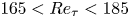 $165< Re_\tau <185$. Indeed, the instantaneous velocity profile figure 22(d) at the chosen times only slightly deviates from the Newtonian flow, represented by blue symbols in the figure.
Let us now consider the EVP flow where both elastic and plastic effects are significant. It is remarkable to see that the EVP flow (figure 22e) behaves like the VE flow, with significant drag reduction in the hibernation regime. Interestingly, the elastic characteristics of the intermittent turbulent dynamics are even stronger for the EVP flow than for the VE flow as also observed in the velocity profiles. The profiles near the active regime (instants i and v) are similar to LDR profiles, whereas the ones under hibernation are more like a HDR, with instant (iv) being very close to the Virk profile. Correspondingly, since the EVP flow hibernates longer periods, we observe a more significant drag reduction (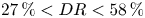 $27\,\%< DR <58\,\%$) than for the purely viscoelastic flow. It is worth noting that we observed and compared several hibernation cycles in VE and EVP flows, in addition to the ones shown in the figure.
We also examine the instantaneous profiles of the mean polymer extension, wall-normal and shear components of the conformation tensor for VE and EVP flow in figure 23. The polymer extension is maximal in the active regime (black and red lines), while it is minimal in the hibernation phase (orange and green lines). The same was observed in viscoelastic turbulent flow in a minimal channel (Xi & Graham Reference Xi and Graham2010, Reference Xi and Graham2012b). While the qualitative picture is the same for VE and EVP, they do present some differences. It appears that at hibernation, the EVP flow has larger polymer extension and higher values of the wall-normal component than the VE flow, while the shear component of the EVP flow is lower, which explains drag reduction. On the other hand, the VE flow presents higher values of both components in the active turbulence regime. (We recognise that these profiles are only snapshots and may not represent accurately the whole dynamics.) EVP stresses are lowest in the hibernation state, and consequently, the probability  $P_s$ of the fluid to be unyielded is highest in the hibernation state, as shown in figure 24. The
  $P_s$-curves neatly divide into two distinct groups in active vs hibernating state, as characterised by
  $Re_{\tau }$, and also by the wall-normal component of the confirmation tensor
  $C_{22}$.

Figure 23. Hibernation phenomenon of VE and EVP fluids, at the same time instants as in figure 22. Mean polymer extension, wall-normal  $\bar {C}_{22}$ and shear
  $\bar {C}_{12}$ components of the mean conformation tensor for VE (
 $Wi=16$ and
  $Bi=0$, a,c,e) and EVP (
 $Wi=8$ and
  $Bi=2.8$, b,d,f) cases.

Figure 24. Probability of the fluid being unyielded in EVP flow ( $Wi=8$ and
  $Bi=2.8$), at the same time instants as in figures 22 and 23.
4. Flow structures
The EVP character of the flow affects the near-wall turbulent structures, and this is visually confirmed in figure 25. In the figure we identify the low- (blue) and high-speed (red) near-wall streaks with isosurfaces of the streamwise velocity fluctuations  $u'$ corresponding to the levels
  $u'^+ = \pm 0.25 U_b$ for the values of
  $Bi$ and
  $Wi$ pertaining all the turbulent cases we have studied. In the Newtonian case (
 $Bi=0$ and
  $Wi=0$), we recognise in the shape of the streamwise velocity fluctuations the typical footprints of the near-wall streaks and quasi-streamwise vortices that characterise the near-wall turbulence and that are responsible for the wall cycle that can sustain turbulence in classical wall-bounded flows (Jiménez & Pinelli Reference Jiménez and Pinelli1999). In VE flows (the leftmost column in figure 25), as the elasticity increases, the low- and high-speed streaks become less fragmented, are correlated over longer distances in the streamwise direction and grow in size. This behaviour has been recognised in the past by several authors (Warholic et al. Reference Warholic, Massah and Hanratty1999; Escudier, Nickson & Poole Reference Escudier, Nickson and Poole2009; Shahmardi et al. Reference Shahmardi, Zade, Ardekani, Poole, Lundell, Rosti and Brandt2019; Le Clainche et al. Reference Le Clainche, Izbassarov, Rosti, Brandt and Tammisola2020) who consistently reported that the inclusion of the polymers in the flow strongly modifies the near-wall structures, by overall enhancing the streamwise coherence of the flow and by increasing the size of the low- and high-speed streaks, thus also moving the quasi-streamwise vortices away from the wall.

Figure 25. Isosurfaces of instantaneous streamwise velocity fluctuation  $u'$ for different Bingham and Weissenberg numbers. The flow goes from left to right and the colour scale ranges from
  $-0.25U_b$ (blue) to
  $0.25U_b$ (red). The green planes in all the figures represent the rigid wall.

Figure 26. The  $x$–
$x$– $z$ planes at
  $y=0.15h$ showing contours of the polymer extension
  $\sqrt {\textrm {Tr}(\bar {C})}/L$ (the colour scale goes from black to white). The blue and red isolines shows the streamwise velocity fluctuations
  $\pm 0.25U_b$. The top row shows cases with increasing
  $Wi=2,4,8$ and 16 from left to right at fixed
  $Bi=0$, while the bottom row cases with increasing
  $Bi=0,2.8$ and 5.6 at fixed
  $Wi=2$. In the figures, the flow is from bottom to top.
A similar modification of the near-wall structures was found by Rosti et al. (Reference Rosti, Izbassarov, Tammisola, Hormozi and Brandt2018c) for the near-viscoplastic case with  $Wi \approx 0$ when increasing the Bingham number. Indeed, the figure clearly shows that the structures in the buffer layer are less fragmented and more elongated in the streamwise direction, as the Bingham number increases. Increase in
  $Wi$ and
  $Bi$ both result in the growth in size of the larger scale structures, which is consistent with an attenuation of the small-scale features of the flow and the consequent reduction of the turbulent dissipation previously observed. This results in a reduction of the friction Reynolds number
  $Re_\tau$, i.e. drag reduction, similarly to what observed in other drag-reducing flows, such as riblets and anisotropic porous walls (Choi, Moin & Kim Reference Choi, Moin and Kim1993; Rosti, Brandt & Pinelli Reference Rosti, Brandt and Pinelli2018b). Although the modifications of the flow structures with
  $Wi$ and
  $Bi$ are similar, some differences are present. Indeed, plasticity alone in VP flows reduces the wall-normal fluctuations less than elasticity because the hibernating turbulent phases are reduced; this results in stronger ejection events and in turbulent structures that penetrate deeper in the bulk of the channel for high values of
  $Bi$. This difference is related to the presence of the unyielded region in the plastic cases, which is inherently intermittent and induces larger values of EVP dissipation rates
  $\varPi$ than in the viscoelastic cases (figures 16d and 19d). Because of this, the drag reduction due to the plasticity is able to laminarise the flow while the one of elasticity is not. The two effects mix in a non-trivial way when both finite elasticity and plasticity are considered. In the EVP cases, the flow structures continue to become less fragmented and more streamwise coherent, with their wall-normal size depending on the relative magnitudes of
  $Wi$ and
  $Bi$. Indeed, as also shown in figure 9, the unyielded region shows a complex trend with
  $Wi$ and
  $Bi$, and this might influence the size of the flow structures. The flow always laminarises at high enough Bingham numbers. However, the VP flow is laminar at
  $Bi>2.8$, showing purely plastic turbulence, while the EVP flow at
  $Wi=2$ becomes laminar only at
  $Bi>5.6$, and hence the turbulence shows combined elastic and plastic characteristics. At high
  $Wi$ (
 $Wi=16$), the trend is reversed and the flow laminarises again at
  $Bi=2.8$, and the effect of plasticity on the turbulent viscoelastic flow is not large due to an early relaminarisation. This non-monotonic trend can be observed in figure 7.
The different effect of elasticity and plasticity on the turbulent flow can be better appreciated in figure 26 where we show wall-parallel contours of the instantaneous polymer extension  $\sqrt {\textrm {Tr}(\bar {C})}/L$ at
  $y \approx 0.15h$, together with the footprints of the low- and high-speed streamwise velocity streaks on the plane. In the top row of the figure we consider the viscoelastic cases with
  $Bi=0$ and growing Weissenberg number
  $Wi$ from
  $2$ to
  $16$. The figure confirms that as
  $Wi$ grows, the polymer extension is enhanced, resulting in more elongated and streamwise coherent structures. Also, it is evident from the figure that the flow structures grow in size, especially the low-speed ones. The second row depicts the results for a fixed Weissenberg number (
 $Wi=2$) and growing Bingham number from
  $0$ to
  $5.6$. Again, we note that as
  $Bi$ increases in the EVP flow, the flow becomes more ordered and streamwise coherent, however, from the figure we can also appreciate the different effect of elasticity and plasticity on the EVP flow: plasticity reduces the turbulent dissipation and the fragmentation of the turbulent structures, acting on both the low- and high-speed streaks equally. Indeed, both appear more elongated in the streamwise direction as
  $Bi$ increases, with only a small growth in their spanwise dimension. On the other hand, elasticity affects mostly the low-speed streaks, while the high-speed ones remain fragmented despite growing in size. A common feature between the two flows is the tendency of the low-speed streaks to appear in regions where the polymers are highly elongated, while the high-speed streaks mostly appear in regions where polymers are not stretched.
5. Conclusions
The combined effect of finite Weissenberg and Bingham numbers in EVP flows has been investigated by direct numerical simulations in this work, and compared with the two limiting cases of VE and VP flows, where VP refers to the near-viscoplastic limit ( $Wi=0.01$) analysed in our previous work Rosti et al. (Reference Rosti, Izbassarov, Tammisola, Hormozi and Brandt2018a). We study both laminar and turbulent flows, where the turbulent case has
  $Re_{\tau }=180$ in the Newtonian limit. A wide range of Weissenberg and Bingham numbers is investigated in this work:
  $Wi=0 - 16$ and
  $Bi=0 - 24$.
Previously, we observed that the VP flow has a moderate drag reduction compared with Newtonian flow at intermediate Bingham numbers, while at higher Bingham numbers the flow relaminarises and drag increases. However, the EVP flow at finite Weissenberg numbers achieves higher drag-reduction values, up to 70 $\%$, than both viscoplastic and viscoelastic flows at the same
  $Re$ and
  $Wi$. Moreover, the drag of EVP flow keeps decreasing after relaminarisation at high Bingham numbers.
The VP flow became laminar at  $Bi \ge 2.8$. The EVP flow is still turbulent at
  $Bi=5.6$ at moderate
  $Wi$, but becomes laminar at
  $Bi=5.6$ for higher
  $Wi$ (
 $Wi\ge 8$). The moderate value of
  $Wi$ triggers instabilities that reinstate turbulence, since the thickness of the unyielded central plug region is considerably reduced compared with the viscoplastic case. At higher
  $Wi$, the central plug region becomes too thin to create instabilities leading to laminarisation.
When analysing the flow statistics, the streamwise component of Reynolds stress tensor increases while the other components decrease compared with the Newtonian flow. This effect is seen for EVP, VE and VP flows. However, it is strongest for the EVP flow. At  $Wi=4$,
  $Bi=5.6$ the components of the EVP flow deviate more from the Newtonian case than VE flow at
  $Wi=16$, or any of the turbulent VP cases.
To characterise the intermittent dynamics relating to the drag-reducing property of polymeric flows (Xi & Graham Reference Xi and Graham2010, Reference Xi and Graham2012b), we divided each flow into hibernating time intervals and periods of active turbulence. The VE flow at  $Wi=16.0$ and
  $Bi=0$, EVP flow at
  $Wi=8.0$ and
  $Bi=2.8$ and VP flow at
  $Wi=0.01$ and
  $Bi=1.4$ were considered. The VP flow showed hibernation phenomenon with small drag-reduction variation. However, the EVP flow hibernates more than any of the others, with the velocity profile reaching close to the Virk profile. All EVP stress components were highest in active turbulence and lowest in hibernation stages. The probability of the fluid to be unyielded was clearly divided into two stages: low probability in active stages and high probability in hibernation.
Finally, we analysed the spatial flow structures and related them to the local elongation of the polymers. As previously noted, both elasticity and plasticity increase the streamwise coherence in the flow. In the EVP flows, we observed that polymer elongation increases with increasing Bingham number, again showing that elastic effects are stronger at finite Bingham numbers than in a purely elastic flow. In both VE and EVP flows, low-speed streaks appear in regions where polymers are more stretched, and high-speed streaks in regions where polymers are less stretched. However, plasticity in EVP flows reduces the turbulent dissipation and hence the fragmentation of both the low- and high-speed streaks equally, while in VE flows high-speed streaks remain fragmented.
Funding
D.I. and O.T. were supported by the European Research Council Grant no. ERC-2019-StG-852529, MUCUS, and by the Swedish Research Council grants No. VR2013-5789 and No. VR2017-0489. L.B. was supported by the European Research Council Grant no. ERC-2013-CoG-616186, TRITOS and by the Swedish Research Council Grant no. VR 2014-5001. L.B. and O.T. also acknowledge the support from the Swedish Research Council via the multidisciplinary research environment INTERFACE, Hybrid multiscale modelling of transport phenomena for energy efficient processes and the Grant No. 2016-06119. The authors acknowledge computer time provided by SNIC (Swedish National Infrastructure for Computing).
Conflict of interest
The authors report no conflict of interest.
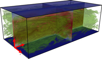


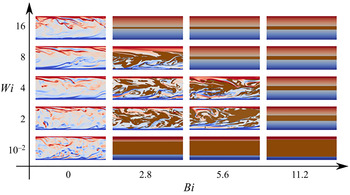


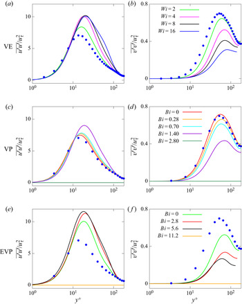


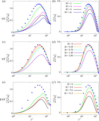


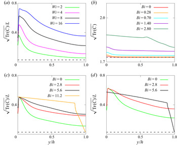


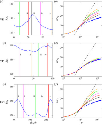


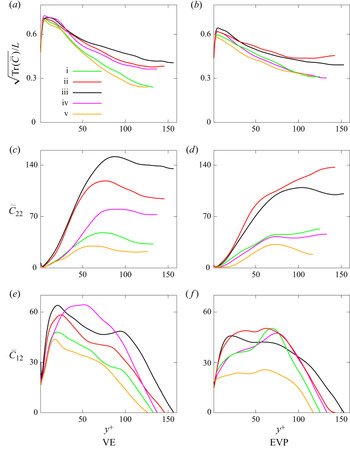


 Open access