


Introduction
Dry permafrost, defined as ground that never warms > 0°C and has a negligible ice content, is rare on Earth. In the high elevations of the Antarctic Dry Valleys, there is dry permafrost with no ice below (Campbell & Claridge Reference Campbell and Claridge2006, Bockheim et al. Reference Bockheim, Campbell and McLeod2007), as well as dry permafrost overlying ice-cemented ground (McKay et al. Reference McKay, Mellon and Friedmann1998, Campbell & Claridge Reference Campbell and Claridge2006, Bockheim et al. Reference Bockheim, Campbell and McLeod2007). Year-round atmospheric and subsurface temperature measurements by McKay et al. (Reference McKay, Mellon and Friedmann1998) at Linnaeus Terrace in Upper Wright Valley at an elevation of 1600–1650 m indicated dry permafrost extending from 12.5 cm below the surface to the top of the ice-cemented ground at 45 cm. Dry permafrost over ice-cemented ground has also been reported near Mount Dolence in Ellsworth Land (Schaefer et al. Reference Schaefer, Michel, Delpupo, Senra, Bremer and Bockheim2017, McKay et al. Reference McKay, Balaban, Abrahams and Lewis2019).
Dry permafrost results when the average frost point at the surface is lower than the average frost point of ice-cemented ground below the surface while the temperature remains < 0°C year-round. This causes any ice that is already present to sublime into the atmosphere and retreat deeper, leaving a dry permafrost soil layer; or conversely ice cannot deposit into these soils as it is unstable. The frost point decreases with depth (McKay Reference McKay2009), and the ice table will stabilize at a deeper level. Initial assessments of the stability of the ice table in the upper Dry Valleys assumed that the atmospheric boundary condition determined the stability of the ice. However, recent work has shown that the effective frost point of the top of the soil column can be different from the atmosphere due to the presence of frost and snow or due to increased moisture content. The temperature and moisture conditions at the surface determine the depth and stability of the ice; the surface conditions are controlled by but not equal to the atmospheric values (Hagedorn et al. Reference Hagedorn, Sletten and Hallet2007, McKay Reference McKay2009, Liu et al. Reference Liu, Sletten, Hagedorn, Hallet, McKay and Stone2015, Fisher et al. Reference Fisher, Lacelle, Pollard, Davila and McKay2016, McKay et al. Reference McKay, Balaban, Abrahams and Lewis2019).
University Valley (77°52'S, 160°45'E; ~1700 m above sea level), one of the upper valleys in the Quatermain Range in the Dry Valleys, is of particular interest in the study of dry permafrost because observations there indicate that the average depth to ice-cemented ground increases linearly across the length of the valley floor (~1.5 km) from near zero to over 1 m (McKay Reference McKay2009, Marinova et al. Reference Marinova, McKay, Pollard, Heldmann, Davila and Andersen2013). This provides a natural experiment regarding the environmental conditions that determine the ice content and temperature regime of dry permafrost. The conditions that allow for ice-cemented ground to reach the surface in these arid and dry locations are not well understood.
In this paper, we report on the climate conditions at University Valley as determined by 3 continuous years of observations of the atmosphere, surface and subsurface dry permafrost and underlying ice-cemented ground. The data were collected from one full meteorological station and three smaller permafrost stations, with the four data collection sites distributed in the Valley (Fig. 1) and having different depths to ice-cemented ground. We also compare this site to other locations in the Dry Valleys for which extensive environmental data exist.

Fig. 1. a. Location of University Valley, Antarctica. b. Aerial photograph of University Valley and the locations of the meteorological weather station (W) and smaller stations over locations of deep (D), medium-depth (M) and shallow (S) ice-cemented ground; yellow bars show elevations in metres. North is up. c. The meteorological station setup.
Lacelle et al. (Reference Lacelle, Lapalme, Davila, Pollard, Marinova, Heldmann and McKay2016) incorporated this University Valley dataset in a comparison of the relations between solar radiation and air and ground temperatures in University Valley and nearby Beacon Valley with those in ice-free Victoria Land and Arctic Canada, focusing their analysis on thermal offset factors.
In this analysis, we develop a detailed energy balance model and use the observational data to constrain the model parameters. Key energy balance model parameters such as albedo and emissivity, but especially thermal diffusivity and roughness length scales, are not well known for the high-elevation Dry Valleys, and this modelling approach develops a way to predict and study surface and subsurface conditions based on limited (past or future) datasets. The model uses atmospheric (temperature, humidity, wind) and solar insulation inputs to determine the surface and subsurface temperature profiles in University Valley. The model can be validated by comparing its results to the measured ground temperatures. The model is used to explore the sensitivity of surface and subsurface conditions to varying environmental properties, corresponding with the natural variability observed within a single valley and at nearby locations. In addition, we examine the changes to the environmental conditions and parameters that would be required to reach key inflection points where the environmental regime changes, such as temperatures above freezing occurring and allowing the presence of liquid water. The presence of liquid water specifically has key implications for habitability and weathering processes.
The model is analogous to that developed by Hunt et al. (Reference Hunt, Fountain, Doran and Basagic2010) for the lower elevations in the Dry Valleys. Hunt et al. (Reference Hunt, Fountain, Doran and Basagic2010) developed an energy balance model for soil temperature and water percolation on the valley floor of Taylor Valley patterned after standard approaches for bare soils without significant vegetation (Matthias Reference Matthias1990). The water balance included snowmelt, freezing/thawing of soil water, soil capillary flow and vapour flows. By computing the surface fluxes of sensible heat exchange between the atmosphere and ground surface, subsurface heat conduction and shortwave and longwave radiation, the model could account for 96–99% of the variation in soil temperature. A significant simplification compared to the model of Hunt et al. (Reference Hunt, Fountain, Doran and Basagic2010) is that, unlike the floor of Taylor Valley, liquid water movement or freezing in the soil column is not important at University Valley. Ice and water vapour are present and exchange by sublimation and condensation (e.g. Lacelle et al. Reference Lacelle, Davila, Fisher, Pollard, DeWitt and Heldmann2013). A complexity of our problem compared to that of Hunt et al. (Reference Hunt, Fountain, Doran and Basagic2010) is determining the properties of the dry permafrost layer, in particular the thermal diffusivity as the temperature and moisture content vary.
University Valley is of special interest as an analogue for Mars environmental and habitability studies. While dry permafrost is rare on Earth, it is widespread on Mars, where dry permafrost begins at the surface and is underlain by ice-cemented ground (Mellon & Jakosky Reference Mellon and Jakosky1993, Mellon et al. Reference Mellon, Arvidson, Sizemore, Searls, Blaney and Cull2009, Smith et al. Reference Smith, Tamppari, Arvidson, Bass, Blaney and Boynton2009, Mellon & Sizemore Reference Mellon and Sizemore2021). The Antarctic Dry Valleys represent one of the driest and coldest places on Earth, and as such they provide an interesting comparison point to conditions in the Martian subsurface. We make this comparison based on the temperature and water activity limits defined for Special Regions on Mars (Rummel et al. Reference Rummel, Beaty, Jones, Bakermans, Barlow and Boston2014).
Methods
Meteorological measurements
A full meteorological station and three smaller permafrost stations were deployed in University Valley on 11 December 2009, including air, surface and subsurface instruments. Data were collected through 31 January 2013. The overall site and the specific locations of the stations are shown in Fig. 1. As can be seen in Fig. 1, all four stations are between 1650 and 1700 m elevation on rocky ground on the valley floor.
The meteorological station is at 77°51.729'S, 160°42.606'E, elevation 1677 m, and it is based on a Campbell CR1000 data logger operated by solar-recharged batteries. The air temperature and relative humidity (RH) were measured 1.2 m above the surface with a Campbell 207 probe in a ventilated radiation shield, as can be seen in Fig. 1. Wind was recorded using an RM Young 05103 wind anemometer (wind speed and direction, 1.08 m above ground) and solar insolation was recorded using a LI-COR sky radiation pyranometer (LI200X, 1.27 m above ground). In the (sub)surface, Campbell 107 temperature probes were placed at the surface (covered with a thin layer of soil), at 10 cm depth, at the top boundary of the ice-cemented ground (42 cm depth) and at 7 cm into the ice-cemented ground (49 cm depth from soil surface). Three Onset U23 Pro v2 External Temperature/Relative Humidity loggers were also placed at the meteorological station site to measure temperature and humidity at the surface (covered with a thin layer of soil), at 20 cm depth and at the ice-cemented ground interface at 42 cm depth. All Campbell instruments were sampled every 30 min, while all Onset sensors were sampled every 60 min (due to limitations in memory capacity). The deep, medium-depth and shallow ice-cemented ground stations were placed in locations with ice depths of 36, 22 and 8 cm, respectively. Their respective locations are 77°51.946'S, 160°43.720'E (elevation 1697 m), 77°51.773'S, 160°43.527′E (elevation 1661 m) and 77°51.584′S, 160°43.019′E (elevation 1684 m). Each site has a combination of an Onset 4 channel smart logger (U12-008) and U23 Pro v2 External Temperature/Relative Humidity loggers with sensors at/close to the surface, halfway to the ice-cemented ground and at the ice-cemented ground interface.
The complete processed datasets are archived at the National Snow and Ice Data Center.
The placement of the probes aimed to minimally disturb the soil and ensure good thermal connectivity with the soil. A narrow hole was manually dug at each site. The surface sensors were placed ~30 cm from the hole, slightly depressed into the ground and covered with a thin layer of soil, aiming to ensure that the surface albedo was maintained. As will be discussed later, the removal of this overlying material by wind and exposing the probe surface directly to the sun may contribute to some non-representative temperature measurements. Sensors in the dry permafrost were inserted 5–10 cm into the side of the dug hole, aiming to minimize the soil disturbance. For the probe in the ice-cemented ground, a hole was drilled using a drill bit with the same diameter as the sensor; the sensor was then snuggly inserted into the hole, ensuring good thermal contact.
The operating temperature range for the Campbell system is -50°C to 50°C, which encompasses the experienced temperature range. The error in the temperature measurement of the 207 and the 107 probes is ±0.2°C. The error in the humidity measurement is < 10%. An important caveat is that the Campbell 207 RH sensor has high errors for RH values < 15%, usually tending to systematically overestimate values; the measured humidity, however, rarely drops to < 30%. The LI-COR LI200X is a solar pyranometer that is sensitive between 400 and 1100 nm with an absolute error in natural daylight of ±5% maximum (±3% typical). The RM Young 05013 Wind Monitor has a stated measurement range of 0–100 m s-1 with a threshold of 1 m s-1 and an error in speed of ±0.3 m s-1 or 1% of the value. The range of directions is 0–360°, with an error of ±3°.
For the Campbell data, the weather station battery value stayed within working limits, including through the winter, reaching a low of 12.2 V and increasing to 14.5 V in summer, supporting the integrity of the data. Full datasets, spanning from 5 December 2009 to 31 January 2013, are available for air temperature and humidity, solar insolation, wind speed and direction and temperatures at 10, 42 and 49 cm depths. The surface temperature is only available for 11 December 2009 to 8 December 2010 and from 26 April 2012 to 11 December 2012; this is the temperature sensor used in all cases in this paper when surface temperature is reported.
For the Onset U23 Pro v2, which is a combined humidity and temperature probe, the operating range is -40°C to 70°C. The error estimates for the temperature sensor are listed as ±0.25°C from -40°C to 0°C and ±0.2°C from 0°C to 70°C. The resolution of the temperature data is 0.04°C. Drift is < 0.01°C per year. Because the temperature-sensing element is a 10 kΩ thermistor, we assume that the main source of error is due to systematic offsets and not random noise. Hence, the error in average values is not significantly decreased with increased sample size. The accuracy of the RH sensor is ±2.5% in the 10–90% RH range and ±5% at < 10% or > 90% RH. The resolution of the sensor is 0.05% and its expected drift is < 1% per year. At temperatures < -20°C or > 95% RH, an additional error of 1% may be present.
For the Onset data, battery information is available for the first year of operation and stays within an appropriate operational range of 3.21–3.56 V. Full datasets, spanning from 5 December 2009 to 31 January 2013, are available for 20 cm depth temperature and humidity and 42 cm depth temperature and humidity. For the surface temperature and humidity, data are available from 10 December 2009 to 4 December 2010 plus some additional short periods of data near the end of the recorded period. The surface humidity data measured by this Onset sensor are used in all cases reported here.
The temperature data at the surface and 42 cm depth were recorded by both the Campbell and Onset sensors. For the surface data, during sunny summer times, the Onset sensor recorded a temperature on average 0.19°C lower than the Campbell sensor, while in winter, the Onset sensor recorded a temperature on average 0.14°C higher than the Campbell sensor. The standard deviations were 0.10°C and 0.13°C, respectively. The maximum differences in temperature were notably higher during the sunny summer times. This is attributed to either or both sensors becoming partially or fully uncovered at the surface by wind moving the thin layer of soil that was placed over the sensors and the Campbell probe having a shiny metallic sensor tip while the Onset sensor has a white tape tip. At 42 cm depth, at the ice-cemented ground interface, on average the Onset sensor recorded a temperature 0.24°C higher than the Campbell sensor, with a standard deviation of 0.13°C. The minimum and maximum deviations were -0.17°C and 0.61°C, respectively.
At the deep (36 cm), medium-depth (22 cm) and shallow (8 cm) ice-cemented ground stations, we also used the Onset U12-008 four-channel outdoor/industrial data logger with the Onset TMCx-HD temperature sensors. The U12 logger has a listed operating range of -20°C to 70°C, but previous experience had demonstrated its operation at lower temperatures. The temperature probes themselves have a measurement range of -40°C to 50°C in soil. The TMCx-HD probe used with the U12 logger has an accuracy of ±0.25°C at 20°C, a drift of < 0.1°C per year and a resolution of 0.03°C at 20°C.
The collected data were checked for integrity. The most notable deviation is periods of missing data, the cause of which is not well understood. Additionally, the Campbell data were corrected for ~5 or fewer points out of a total dataset of > 55 000 data points per sensor. These errant values were probably due to cosmic ray strikes. An exception was the surface temperature, which had ~5% of data points removed due to unrealistically high values (e.g. > 20°C, where this cannot be explained by surface property variation such as rocks) and also had extensive stretches of missing data.
For minimum and maximum temperatures and thaw depths, the instantaneous readings are reported. For the modelling, a time step of 1–2 min was used.
Relative humidity correction and drift
The sensor in contact with the ice table provides a useful test of the response of the humidity sensor, as it is expected to show a constant 100% humidity. McKay et al. (Reference McKay, Balaban, Abrahams and Lewis2019) used similar sensors to define the correction needed to determine the humidity values at temperatures below freezing. Anderson (Reference Anderson1994, Reference Anderson1995) and Koop (Reference Koop2002) assumed that RH sensors record the RH with respect to liquid water even for temperatures < 0°C, and previous work (e.g. Doran et al. Reference Doran, McKay, Clow, Dana, Fountain, Nylen and Lyons2002, Hagedorn et al. Reference Hagedorn, Sletten and Hallet2007, Andersen et al. Reference Andersen, McKay and Lagun2015, Liu et al. Reference Liu, Sletten, Hagedorn, Hallet, McKay and Stone2015) used this assumption in correcting Antarctic data. The RH data from the University Valley Campbell 207 probe are corrected this way. However, McKay et al. (Reference McKay, Balaban, Abrahams and Lewis2019) found that the results from the Onset sensors at the ice table indicated a correction of
 $$RH_i = RH_w- 2 - 0.65T$$
where RHi is the RH over ice, RHw is the sensor reading (approximately the RH over water) and T is the temperature in degrees Celsius. When corrected using this method, our data for the ice table are consistent with a RH of 100% within approximately ±1% (see Appendix).
The 3 year duration of our dataset with the RH sensors undisturbed allows for an assessment of the drift of the sensors over time. We find that the sensor drift is an increase in the indicated reading of < 1% per year (see Appendix). Nair et al. (Reference Nair, McCarthy, Heusch and Patz2015) tested the response of humidity sensors stored for 7 months at room temperature and tested at RH values from 30% to 70%. They reported errors of 0.4% ± 0.2% RH (n = 5 sensors). If the sensing film is stable, then the primary cause of sensor ageing when exposed to air is the accumulation of contaminant particles on the sensor material, changing its properties and response time (Nair et al. Reference Nair, McCarthy, Heusch and Patz2015 and references therein). The constant low-temperature environment of the ice table, with little or no airborne particulates, may minimize sensor drift.
Ground energy model
The energy balance model uses as inputs the local environmental conditions and calculates the surface and subsurface temperatures, which can then be compared to the measured values. The model can be forced using flux boundary conditions at the top and bottom or with enforced temperature boundary conditions to calculate the temperature profile in the in-between layers. In the case of a flux forcing at the top, we nominally use the values measured at the site; however, the flux can also be calculated using representative theoretical values (such as expected solar insolation based on the location of the site and air temperature based on an average temperature and idealized diurnal and yearly fluctuations). The values used for all constants are described here and in more detail later.
The flux of heat at the surface is given by:
 $$F_{surf} = Solar + Longwave + Sensible + Latent-Blackbody$$
where Fsurf is the net flux at the surface (W m-2), Solar is the net incident solar radiation, Longwave is the net longwave sky radiation, Sensible heating is due to turbulent heat transfer between the surface and air, Latent heating is due to turbulent heat flux from the movement of water vapour between the surface and air and Blackbody is the blackbody radiation from the surface. We set downwelling radiation (i.e. energy that is added to the surface) as positive, except in the case of Blackbody, which is always positive and denotes energy radiated from the surface. In solving for the subsurface temperatures, Fsurf sets the upper boundary condition, and the lower boundary condition is set to no net flux.
Solar is given by the solar flux (Ssurf) measured by the weather station (W m-2) or as calculated by the sun model and adjusted for the surface albedo, or reflectivity, A, at the site of interest:
 $$Solar = ( {1-A} ) S_{surf}$$
Longwave is given by (as used by Mölg & Hardy Reference Mölg and Hardy2004):
 $$Longwave = \sigma T_{air}^4 ( {C_1 + C_2E_{air}} ) ( {1 -shadow} ) $$
where σ is the Stefan-Boltzmann constant (5.67 × 10⁻⁸ W m-2 K-4), Tair is the air temperature (K), C1 and C2 are fitting parameters, which are set to 0.585 and 6.2 × 10⁻⁴ Pa-1, respectively, following Mölg & Hardy (Reference Mölg and Hardy2004), and Eair is the water vapour partial pressure (Pa). A shadowing term, shadow, takes into account that the surrounding valley walls limit the surface from seeing the full sky.
The sensible heat flux, Sensible (W m-2), is given by:
 $$Sensible = C_{\,p, air}\rho _0\displaystyle{P \over {P_0}}\displaystyle{{K^2v( {T_{air}\;-\;T_{surf}} ) } \over {ln\left({\displaystyle{{z_m} \over {z_{0m}}}} \right)ln\left({\displaystyle{{z_h} \over {z_{0h}}}} \right)}}$$
where Cp,air is the heat capacity of air (J kg-1 K-1), ρ0 is the density of air at standard temperature and pressure (kg m-3), P is the local air pressure (Pa), P0 is the air pressure at STP (Pa), K is the von Kármán constant, v is the wind velocity (m s-1), which is taken from the measured wind velocity at the weather station, Tair is the air temperature (K), Tsurf is the surface temperature (K), zm is the height at which the wind measurement is taken (m), z0m is the momentum roughness length scale (m), zh is the height of the air temperature measurement (m) and z0h is the roughness length scale of temperature (m). The atmospheric pressure is assumed (not measured) to be constant and proportional to the altitude: P = 82.8 kPa for University Valley.
The latent heat flux, Latent (W m-2), is calculated using:
 $$Latent = 0.623L_{sublime}\rho _0\displaystyle{1 \over {P_0}}\displaystyle{{K^2v( {E_{air}\;-\;E_{surf}} ) } \over {ln\left({\displaystyle{{z_m} \over {z_{0m}}}} \right)ln\left({\displaystyle{{z_v} \over {z_{0v}}}} \right)}}$$
where Lsublime is the latent heat of sublimation from the ice in the subsurface to vapour in the atmosphere (J kg-1), Eair is the vapour pressure in the air (Pa), Esurf is the vapour pressure at the surface (Pa), zv is the height at which the humidity measurement was taken (m) and z0v is the roughness length scale of water vapour (m). The vapour pressure in the air is calculated using the measured RH. For the surface, the water vapour pressure is calculated using the measured surface humidity when depth of ice-cemented ground (dice) > 20 cm. However, in the case where the ice depth is 3 cm or less, the surface humidity is set to 100%, as the surface is effectively in contact with the ice. For ice depths between 3 and 20 cm, the surface humidity is linearly interpolated so that it equals 100% when dice = 3 cm and it equals the measured surface RH when dice = 20 cm.
The blackbody radiation is given by:
 $$Blackbody = \varepsilon \sigma T_{surf}^4 ( {1 -shadow} ) $$
where ɛ is the emissivity of the surface and Tsurf is the surface temperature (K). The shadowing by the surrounding cliffs, shadow, as also used in the equation for Longwave radiation, accounts for the surface not radiating to the cold sky in all 2π steradians due to the surrounding valley walls. The temperature of the surface of the cliffs is assumed to be close to that of the measurement site. Only in the case of Blackbody does a positive value denote energy being lost by the surface; note that Solar and Blackbody always have positive or null values. For all other terms in the energy balance equation, positive values denote energy being deposited into the ground.
When fitting parameters or determining how well a certain modelling run fits the data, we use as input the measured solar flux, calculate the longwave radiation from the measured temperature and air humidity, calculate the sensible and latent heat fluxes using the measured air properties and the calculated surface properties and calculate the blackbody radiation from the calculated surface properties.
Numerical method
Below the surface, we solve the thermal diffusion equation (Eq. (13) in the Appendix) using the Crank-Nicolson method (Acton Reference Acton1970). This numerical method is a combination of the forward Euler and the backward Euler methods, is implicit in both the time and spatial variables and is generally stable for diffusion equations. The radiative, convective and conductive fluxes together specify the upper boundary condition. The lower boundary condition is a zero-flux condition (∂T/∂x = 0). We can also set the upper or lower boundary condition to specified temperature values over time, which can be set to the measured values. The key parameter that combines the physical properties of the soil and the numerical spacing of the time and spatial variables is α:
 $$\alpha = \displaystyle{1 \over 2}\displaystyle{k \over {\rho C_p}}\displaystyle{{\Delta t} \over {\;\Delta x^2}}$$
where k is the thermal conductivity (W m-1 K-1), ρ is the density (kg m-3), Cp is the heat capacity (J kg-1 K-1), Δt is the time step that is used (s) and Δx is the thickness of each of the modelled subsurface layers (m). The values of k, ρ and Cp are specific to each layer and can change with depth in the simulated subsurface. We thus simulate the dry soil using the designations of ksoil, ρsoil and Cp,soil and the ice-cemented ground using the designations kicy-soil, ρicy-soil and Cp,icy-soil. The smaller the value of α, the more stable the result. The time step used is nominally 120 s, although in some cases it is decreased to 60 s to reduce the possibility of the model developing numerical instabilities. The layer thickness was set to 1 cm.
The model can also be run by enforcing temperature boundary conditions; that is, forcing the top and bottom boundary conditions with specified temperatures rather than setting a flux condition. The model then solves for the in-between temperatures. This approached was used in trying to solve for the soil thermal diffusivity, as will be described below.
Parameters used in the model
One of the benefits of collecting in situ data is the ability to extract or at least confirm that the parameters being used in associated models reasonably represent the environment. The ability to do this is determined by limitations in the collected dataset (number of sensors available, disturbing the site during placement and sensor capabilities and failures) and the challenge of using one or a few measurement locations to meaningfully describe and characterize the complex and varying natural environment. In choosing the environmental parameters to represent the University Valley site, we use a multi-pronged approach: attempting to extract these parameters from the available data, reviewing the literature and using other analytical and empirical fits that have been developed. It should be noted that a first attempt was made to do a large parameter space search in order to determine what combination of values would provide the best fit to the data. This approach did not yield useful results for a number of reasons. Primarily, the limitations of the collected data affect the fitting statistics that are calculated. Additionally, the idea of ‘best fit’ is ambiguous, with there being several statistical measures that could be minimized, including mean absolute error, mean error, median error or ensuring no significant overshoots in summer warm periods (the period arguably of most interest). Each of these criteria leads to a different set of fitting parameters that produce a ‘best fit’. Because of ambiguity in which statistical measure is most important to minimize, we chose to use the combination of targeted fitting and environmental parameter values and methods from the literature. The parameters used in the model are summarized in Table I.
Table I. Nominal model parameters and values used.

Surface albedo
The best fit surface albedo is determined by fitting the surface warming rate during sunny, cloudless and low-wind days. The high solar insolation results in the Solar component of the energy balance equation dominate, while the low wind reduces the sensible and latent heat fluxes. Additionally, fitting the shape of the rise in surface temperature specifically focuses on the solar warming rather than requiring an overall accurate fit. The snow albedo is fit using a similar methodology; we infer that the surface is snow-covered when the surface humidity is high (> 90%) and concurrently the atmospheric humidity is low (< 80%). There are few periods appropriate for snow albedo fitting because snow is not common in summer when solar insolation is high.
Using this methodology and fitting three separate summer periods, the surface albedo at the weather station site is determined to be ~0.33. This albedo is overall consistent with published values (e.g. An et al. Reference An, Hemmati and Cui2017), although it is towards the higher end. Overall, significant variability in albedo values is apparent in the published data. For snow, we determine the albedo to be 0.86, which is a bit low but close to the range of reported values (e.g. Wiscombe & Warren Reference Wiscombe and Warren1980). However, this value has less of an overall impact as snow is not common during high-insolation and warmer summer periods, which are of most interest for this work.
While we do not have a direct measurement of snow cover at University Valley, we infer that snow-like albedo and emissivity should be used when the measured air humidity is < 80% but the surface humidity is > 90% at the weather station site. It is unclear how well this criterion applies to the dark winter months and how often surface frost rather than snow may produce a similar response in humidities; our modelling and the data cannot provide further insight on this point.
Surface emissivity
The surface emissivity was found by fitting winter surface temperatures as the surface is warmed by katabatic winds but then cools during a period of low wind. The low wind as the surface cools minimizes the latent and sensible heat flux contributions and the winter darkness eliminates the solar insolation term. The energy balance equation reduces to a relationship between the blackbody outgoing radiation, which is a function of surface emissivity and dominates, and the incident longwave radiation. The properties of the subsurface also play a role, as they set the rate at which energy diffuses from or into the surface; however, this term did not appear to appreciably affect the best fit emissivity. We find best fit values of ɛsoil = 0.92 (from three fit periods), and we chose ɛsnow = 0.97 to be consistent with the literature (Hunt et al. Reference Hunt, Fountain, Doran and Basagic2010), as the overall low blackbody signal during the cold winter months made fitting snow emissivity challenging.
Shadowing
The shading at the weather station was measured in 10° radial increments using an inclinometer (valley wall profile shown in Fig. 2). The sky fraction (i.e. the fraction of the hemisphere that is sky) is calculated using the equation for the normalized area of a spherical cap: Acap = 2π(1 - sinα), where α is the angle from the horizontal to the horizon. For a hemisphere, α = 0°, and this reduces to Acap = 2π steradians, as expected. To calculate the sky fraction with a valley wall profile that is not at a constant angle, we sum over the measured profile:
 $$Sky = \mathop \sum \limits_{0^\circ \;< \;\theta \;< \;360^\circ } 2{\rm \pi }( {1\;-\;\sin \alpha_\theta } ) \left[{\displaystyle{{\Delta \theta } \over {2{\rm \pi }}}} \right]$$
where θ is the radial angle and Δθ is the radial increment over which the angle α was measured. We then get shadow = 1 - Sky. Using the valley wall profiles shown in Fig. 2, we find the shadowing at the weather station site to be 35.5%.

Fig. 2. Profile of the valley walls from the weather station site in University Valley: 35% of the sky is obscured by the valley walls.
Thermal diffusivity
The parameter that appears directly in the diffusion equation (Eq. (13)) is the thermal diffusivity, κ, which depends on fundamental soil properties: ρ (soil density), C (heat capacity) and k (thermal conductivity) as κ = k/ρC. We derive values of the thermal diffusivity considering several different numerical approaches, as discussed by Pringle et al. (Reference Pringle, Dickinson, Trodahl and Pyne2003), and using direct fitting with the model. These approaches are described in detail in the Appendix. Importantly, we find that the thermal diffusivity is a function of temperature, where κsoil = 6.9 × 10⁻⁷ m2 s-1 for -5°C ≤ T ≤ -25°C and rises from κsoil = 6.9 × 10⁻⁷ to 1.0 × 10⁻⁶ m2 s-1 for T = -25°C to -45°C. The increase in κsoil at low temperatures is probably due to frost cementation of the dry grains, as described in the Appendix, with a smaller effect due to the change in thermal conductivity and heat capacity of mineral grains and ice with temperature. This is directly seen by the strong correlation of thermal diffusivity with humidity increasing to ~100% for temperatures < -25°C and concurrently the thermal diffusivity increasing below this temperature. Using a representative soil density of 1630 kg m-3 and a heat capacity of 800 J kg-1, as per McKay et al. (Reference McKay, Mellon and Friedmann1998), this gives a soil thermal conductivity (ksoil) of 0.9 W m-1 K-1 for -5°C ≤ T ≤ -25°C, and ksoil rises from 0.9 to 1.3 W m-1 K-1 for T = -25°C to -45°C.
For the ice-cemented ground, we use the values published in McKay et al. (Reference McKay, Mellon and Friedmann1998) of κicy_soil = 1.0 × 10⁻⁶ m2 s-1, using their representative density (2022 kg m-3), heat capacity (1200 J kg-1) and thermal conductivity (2.5 W m-1 K-1).
Latent and sensible heat fluxes
The latent and sensible heat fluxes require as input the roughness length scales for momentum, temperature and water vapour. These length scales in effect characterize the turbulent flow that is generated by the surface features at the site: rocks, boulders and vegetation. These values are accordingly specific to the site and can differ by orders of magnitude between sites (e.g. between a smooth glacier surface and a forested area).
The momentum roughness length scale is a measure of the aerodynamic roughness of the surface, while the temperature and water vapour roughness length scales represent the surface height below which the representative surface value is reached for the respective quantity. No measurements of these values, either by profile measurements or sublimation measurements (e.g. Denby & Snellen Reference Denby and Snellen2002, Wagnon et al. Reference Wagnon, Sicart, Berthier and Chazarin2003), have been made for University Valley. We also did not find measurements for surfaces that are similar to the rough and rocky surface of the study site. Mölg & Hardy (Reference Mölg and Hardy2004), in their modelling of the glaciers on Kilimanjaro, used a value of 0.001 m for all three roughness length scales based on measurements at Canada Glacier, Antarctica (Lewis et al. Reference Lewis, Fountain and Dana1999).
Both theoretical and field evidence suggests that the momentum, temperature and water vapour length scales should not be expected to be the same (e.g. Andreas Reference Andreas1987, Greuell & Smeets Reference Greuell and Smeets2001), and generally the temperature and water vapour length scales are similar and one to three orders of magnitude smaller than the momentum roughness length scale (Mölg & Hardy Reference Mölg and Hardy2004). In the case of University Valley, we expect the length scales to be larger than those measured at the glaciers due to the greater roughness of the surface.
The surface of University Valley is covered by material ranging from sand grains to boulders approaching 1 m in height (Fig. 1; also see fig. 3 in Heldmann et al. Reference Heldmann, Pollard, McKay, Marinova, Davila and Williams2013) and patterned ground with polygons that range in size from 10 to 25 m in diameter (Mellon et al. Reference Mellon, McKay and Heldmann2014). Most of the published studies of turbulent heat and momentum transfer in the Antarctic are over ice or snow surfaces that are relatively smooth compared to University Valley.
In the context of aeolian transport of sand, Lancaster (Reference Lancaster2004) conducted a systematic field study of roughness length in a variety of Dry Valley surfaces ranging from flat sand to rocky moraines. For the smoothest surface he derived values of z0m = 0.0009 m, while for the roughest surface he obtained z0m = 0.0360 m. Liu et al. (Reference Liu, Li, Yang, Wang, Wang, Li and Gao2019) computed z0m at Zhongshan Station at a rocky site (see fig. 1 in Liu et al. Reference Liu, Li, Yang, Wang, Wang, Li and Gao2019), inferring a momentum (aerodynamic) roughness length of z0m = 0.0036 m. They computed the thermal roughness length from the momentum roughness length using the approach of Andreas (Reference Andreas1987), obtaining a value of z0h = 0.00012 m and a ratio of z0m/z0h = 30.
For our modelling, we use the rockiest site in Lancaster (Reference Lancaster2004) to set z0m = 0.0360 m. We follow Liu et al. (Reference Liu, Li, Yang, Wang, Wang, Li and Gao2019) in using a ratio of 30 between z0m and z0h, and we follow Andreas (Reference Andreas1987) in setting the temperature and water vapour roughness length scales equal to each other: z0h = z0v = 0.0012 m.
We also tried to independently determine the roughness length scales at University Valley by fitting the data during relevant times. Specifically, after determining the surface albedo, emissivity and subsurface thermal diffusivity, we looked for low-insolation periods with strong winds and sudden changes in wind speeds. This increased the relative importance of the latent and sensible heat fluxes in the energy balance equation. Searching the plausible parameter space, this fitting supported the assumption that the temperature and water vapour roughness length scales are approximately equal and that the values of the roughness length scales selected above are approximately in the middle of the range of well-fitting values.
von Kármán constant
For the von Kármán constant, we use the traditionally accepted value of 0.4 (e.g. Högström Reference Högström1985), but more recently Andreas et al. (Reference Andreas, Claffey, Jordan, Fairall, Guest, Persson and Grachev2006) have suggested that a value of 0.387 may be more accurate. We proceed with using a value of K = 0.4, but note that the lower value will decrease both the latent and sensible heat fluxes by 6.8%. The resulting effects are explored in the sensitivity studies described below.
Longwave radiation
The longwave radiation parameterization that we used is only one of the possible parameterizations. In particular, significant work has been done on the change in longwave radiation parameterization depending on whether the sky conditions are clear or cloudy. In the case of our dataset, we can use apparent atmospheric optical depth to determine cloudy conditions during the sunny months; however, this is not possible for the long, dark winter, when longwave radiation is a more significant component of the radiation budget.
The nominal values used in the modelling are shown in Table I. These values are primarily determined using the methods described above. Where the more general fit suggests a range of values, the ones that preferentially show a good fit during the warm summer days are chosen, as it is during the warm summer days that the question of the availability of water is most important and the surface temperatures peak.
Results
Collected weather data
We recorded 3 complete years of data (2010–2013) at the weather station site (marked with a ‘W’ in Fig. 1). The averages and extrema of temperature and RH are shown in Table II. For each location, the frost point is calculated based on averaging the water vapour density computed from individual values of the temperature and RH (e.g. McKay Reference McKay2009). Table III lists the average sunlight and wind speed, which are important parameters for comparison with other meteorological stations throughout the Dry Valleys. Figure 3 provides an overview of the entire dataset, showing the daily average air temperature, sunlight, RH and wind speed.

Fig. 3. Daily averages for a. air temperature, b. sunlight, c. air relative humidity and d. wind speed at 1.2 m above the surface for the University Valley weather station site. Numerical values are in the Supplemental Material.
Table II. Summary of temperature and humidity data (2010–2013).

a The surface and frost point data could not be calculated for the 2010–2013 dataset directly because of missing data, as described earlier. The reported values are calculated by taking the continuous 358 days of surface temperature and humidity data that was collected using the Onset U23 Pro v2 temperature/relative humidity sensor from December 2009 to December 2010 and repeating the last 7 days again to make a complete 1 year (365 day) dataset. Additional surface temperature data from the Campbell T107 temperature probe are available; however, as these data do not provide full-year datasets, they are not reported in this table.
b A maximum surface temperature of 12.3°C was recorded using the Campbell T107 temperature probe in the summer of 2012.
Table III. Sunlight and wind speed for each year (2010, 2011, 2012).

From the peak temperatures at 10 and 20 cm depths in Table II, we estimate that the depth of the active layer (the maximum depth of the 0°C isotherm) is ~15 cm. Given the variability in conditions across University Valley, this active layer depth is only applicable locally to the weather station site. This compares well to the value of 12.5 cm determined for a similar site (Linnaeus Terrace in Wright Valley; McKay et al. Reference McKay, Mellon and Friedmann1998). Considering all four summers of the dataset, the depth of the active zone varied by 4 cm and the mean was 13.2 ± 2.2 cm.
As can be seen in Table II, the frost point of the surface and the frost point of the ice table 42 cm below the surface are identical, providing direct confirmation that the surface conditions are the relevant boundary conditions for ground-ice stability and not atmospheric conditions measured at 1–2 m above ground height.
Table IV lists the summer monthly averages and extrema of temperature for those summer months for which the data are complete. Figure 4 shows the average wind speed as a function of wind direction and also shows the correlation between air temperature and RH with wind direction and the frequency of wind directions.

Fig. 4. Distributions of a. wind velocity and c. relative humidity (RH) with wind direction, as well as b. frequency of wind directions for the weather station site.
Table IV. Monthly summer air temperature values.

Model validation
We tested the model for fit against the continuous 358 days of surface temperature and humidity data from the Onset temperature/RH sensor from December 2009 to December 2010. Comparing the model and measured surface temperatures, the mean error is 1.3°C, the median error is 1.7°C and the mean absolute error is 2.1°C. By tuning the parameters noted in Table I within their realistic range, this error could be considerably reduced. For example, by reducing the momentum roughness length scale to 0.018 m (from 0.036 m) and setting the temperature and water vapour length scales to be 100 times smaller, the mean error reduces to 0.9°C, the median error reduces to 1.2°C and the mean absolute error reduces to 1.6°C. These possible corrections notwithstanding, we proceed with the values as given in Table I, as they still provide a reasonable fit for surface and subsurface temperatures for the whole year and a very good fit for the summer time period used for the further sensitivity studies, as described next.
We use a reference sunny and warm summer period to assess the fit of the model to the surface and subsurface temperature data (Fig. 5). As described later, this same time period is used to look for the effects of changes of parameters on the surface and subsurface temperatures. In this as in the other cases described, the model uses the atmospheric conditions (air temperature and humidity and wind velocity) and solar insolation as inputs to the energy balance, and the surface and subsurface temperatures are the calculated outputs. The reference period is 7–17 November 2010 (days 310–320). This period is unusual and particularly interesting as it includes multiple days of above-freezing surface temperatures, with a maximum surface temperature of 5°C. The model fits the data for this period quite well, as can be seen in Fig. 5, where the surface temperature has a mean error of -0.4°C, a median error of -0.12°C and a mean absolute error of 1.6°C. The peak temperatures are fit within 1°C. The largest errors are due to small offsets in the rise and fall rate during each day. As the temperature changes sharply when the sun rises or sets behind the valley walls, an offset of just half an hour in the response can produce errors of 5°C in the modelled vs measured temperature. The response time of the temperature sensors may also play a role in these cases. The overall close fit to the data allows for meaningful conclusions to be drawn about temperature changes as a result of varying environmental parameters.

Fig. 5. Reference warm period used for assessing the sensitivity of the environment to changing parameters; data collected at the weather station site. The model fits the data to within a few degrees Celsius, which allows for meaningful assessment of temperature changes when the environmental parameters are varied.
It is important to note, however, that this period does not have the warmest surface temperatures recorded during the 3 years of data collected from the site; the maximum recorded surface temperature was 12°C compared to 5°C in the reference warm period. From the available data, this is also seen in the 10 cm depth temperature measurement; for the period being analysed (up to day 341, as described later), the maximum temperature is -5.5°C, while the overall highest temperatures recorded at this depth during the summers of 2010–2011, 2011–2012 and 2012–2013 are +2.7°C, +2.8°C and +2.5°C, respectively. Thus, the results below should be interpreted specifically regarding the warm period being analysed, but they do provide a useful test of the ability of the model to match warm surface temperatures.
The model is initialized with a subsurface profile approximating this time of the year (confirmed by the subsurface temperature measurements), starting 50 days preceding the start of the reference warm period shown in Fig. 5 (day 260). This ensures that the model has equalized and the subsurface profile is expected to accurately represent the subsurface temperatures. The 50 day damping depth is 97 cm, which extends significantly past the 42 cm dry soil to the ice-cemented ground interface. The model is also run for 21.6 days after the end of the period of interest to allow for the thermal wave to propagate to the ice and for a more accurate maximum ice temperature to be obtained. For 21.6 days, the damping depth is 64 cm; however, the peak of the thermal wave is not expected to reach 42 cm in this timeframe. A longer timeframe is not simulated as this is the last data point that is available for the surface humidity dataset, and running the model further would require extrapolating the humidity data.
Sensitivity of surface and subsurface temperatures to environmental variations
The warm, sunny 10 day period described above (Fig. 5) is used to assess the sensitivity of the surface and subsurface conditions to changing environmental factors (Tables V & VI), with the goal of understanding both the effect of natural variability seen in the local University Valley environment (e.g. surface optical properties and textures) and the effect of variations from year to year and between neighbouring local valleys (e.g. wind profiles and air humidity). In the former case, the fitting parameters, such as albedo, emissivity and roughness length scales, are varied within the reasonable range and assessed uncertainty of the values, capturing the natural variability in the area (as described earlier for each parameter in the ‘Methods’ section). In the latter case, we vary the parameters within a plausible range of year-to-year and local inter-valley variability. The sensitivity studies also point to what parameters are especially important to determine with more certainty in future studies in order to more accurately model local conditions.
Table V. Modelling of the sunny, warm period in November 2010 and how changing local conditions and environmental parameters modifies the surface and subsurface temperatures. Unless otherwise noted, the environmental and subsurface parameters are those described in Table I. In all cases, z0h = z0v. Thaw depth is the depth to which the subsurface is warmed above freezing, regardless of water content.

Table VI. Effect of changing the depth of ice-cemented ground. Unless otherwise noted, the environmental and subsurface parameters are those described in Table I. In all cases, z0h = z0v.

Four quantitative metrics were used to compare the system response to parameter variations: maximum surface temperature, maximum ice temperature, the depth to which the subsurface is warmed above freezing regardless of water content (thaw depth) and the degree days above freezing at the surface (integral of the temperature-time curve for when the surface is above freezing). These quantitative metrics are evaluated as follows: maximum surface temperature and degree days above freezing for days 310–320 and maximum ice temperature and thaw depth during days 310–341.6 (Table V).
For this time period, the baseline model, using the best fit and as-measured environmental properties summarized in Table I, gives a maximum surface temperature of 5.8°C, a thaw depth of 4 cm and a maximum ice temperature (at 42 cm) of -18.9°C. These values are in close agreement with the measured values. The very shallow thaw depth demonstrates how the low thermal diffusivity of the warm, dry soil quickly dampens out the thermal wave. However, as noted earlier, this modelling run is more specific to the timeframe being analysed, and the thaw depth computed here is not to be confused with the depth of the active layer. The depth of the active layer is the maximum thaw depth achieved over the entire summer and, as discussed above, it averages 13.2 cm.
The variation in parameters that may be expected at the site has a moderate effect on the surface temperatures. Specifically, the variations in albedo, emissivity, thermal diffusivity of the soil, wind variability, roughness length scales and solar variability result in up to ~3.5°C warming in the surface temperature and ~1°C warming of the ice-cemented ground at 42 cm, keeping it well below the freezing point. The thaw depth varies by only a few centimetres. The warmest surface results from increasing the solar insolation by ~20%, which is at the upper limit of what may be plausible (i.e. effectively a significant decrease in cloud cover). The highest ice temperature occurs as a result of increasing the thermal diffusivity of the soil, which then allows more of the surface heat to be carried to depth.
The sensitivity to surface albedo is approximately ±1.3°C of the surface temperature for a corresponding change of approximately ±0.05 in albedo. The albedo value is expected to be most strongly affected by the surface material properties, grain size and presence of rocks, with a probably insignificant effect of whether pore-filling ice reaches the surface.
Emissivity changes of ±0.02 result in corresponding surface temperature changes of ±0.2°C.
Wind changes of ±25% result in corresponding surface temperature changes of approximately ±1.8°C, with higher winds making the ground colder. Higher winds result in a stronger coupling between the air and surface temperature, cooling the ground to the air temperature in summer and warming the ground in winter.
Solar flux changes of ±10% result in corresponding surface temperature changes of approximately ±1.9°C.
Changes in the roughness length scales have an effect that is comparable to the values discussed above. Thus, roughness length scales may be important in comparing results between sites with different surface characteristics.
There is an observed change in depth to ice-cemented ground down the length of University Valley. We noted that when the ice-cemented ground is exposed at the surface there was no melting observed during the three summer field visits. In using the model to simulate different ice depths, with all other parameters being as described in Table I, we find a similar result (Table VI): ice-cemented ground at the surface does not melt in the summer. There is some ambiguity in these results as the observation period during a field visit is brief, the modelling does not use the warmest period recorded in the 3 years of data and the warmest temperatures recorded at 10 cm at the weather station site were ~2.5°C, although the data from an ice-cemented ground depth of 42 cm cannot be directly related to temperature profiles when the ice reaches the surface.
Changing the depth of the ice in the model changes the computed subsurface temperature profile dramatically, as expected. Modelling ground ice all the way to the surface gives a maximum surface/ice temperature of approximately -2.5°C. Our measured temperature at the shallowest ice site (depth to ice of 8 cm) gave a maximum ice temperature of -16°C during this same timeframe and a maximum ice temperature for the year of -4°C. Modelling an ice depth of 8 cm at the weather station site gives a maximum ice temperature of -7°C during the modelled timeframe. These results are overall consistent, and some discrepancy is expected as the narrowness of University Valley results in rapidly varying shadowing and solar insolation throughout the valley floor; other environmental factors are expected to vary as well, changing the thermal environment.
It should be noted that to model intermediate depths of ice we must specify a surface humidity value. This is done as described earlier after Eq. (7). As there is uncertainty in how to treat the surface humidity for shallow ice depths, the latent heat component of the energy balance is more uncertain.
Shallower depths to ice-cemented ground increase the thermal diffusivity, which enables heat from the surface to be more easily conducted into the subsurface. In addition, the higher thermal heat capacity of ice-cemented ground results in the same heat input resulting in a smaller bulk temperature increase. Thus, even when ice is present close to what is normally expected to be a warm surface from solar heating, the presence of the ice modifies the subsurface properties in such a way that the ice is still kept below freezing and no melting occurs. This general observation is expected to hold during average years, but exceptional weather excursions can still result in conditions that may melt subsurface ice, particularly for shallower ice. This is discussed further in the ‘Discussion’ section.
Discussion
Climate comparison
To place the climate of University Valley and the conclusions we draw from our data and modelling into the broader context of climate in the Dry Valleys, we compare the overall climate of University Valley to the extensive datasets that exist for other locations in the Dry Valleys. These include early datasets (Keys Reference Keys1980, Clow et al. Reference Clow, McKay, Simmons and Wharton1988), the Long-Term Ecological Research (LTER) network (Doran et al. Reference Doran, McKay, Clow, Dana, Fountain, Nylen and Lyons2002), the stations of the Soil Climate Monitoring Project (Seybold et al. Reference Seybold, Harms, Balks, Aislabie, Paetzold, Kimble and Sletten2009) and the stations established at high elevations to study the cryptoendolithic colonization in the Beacon Sandstone (Friedmann et al. Reference Friedmann, Druk and McKay1994, McKay Reference McKay2015).
The average air temperature at University Valley is -23.4°C, comparable to the values for similar elevations in Wright Valley (Friedmann et al. Reference Friedmann, Druk and McKay1994), and this is only a few degrees colder than the average at some of the low-altitude lake sites near the coast. For example, Doran et al. (Reference Doran, McKay, Clow, Dana, Fountain, Nylen and Lyons2002) report an average temperature at Lake Fryxell of -20.2°C. Comparing University Valley to Lake Fryxell, the long, cold winters at University Valley are not much colder than at Lake Fryxell, but the summer months are much colder. This is due mainly to the effect of elevation on summer air temperature. Lake Fryxell has a peak summer air temperature of 9.2°C and an average of 25.5 degree days above freezing (integrated time during which the air temperature is above freezing). At University Valley, the peak summer air temperature effectively never gets above zero; there are no summer degree days above freezing. Over the 3 year data period, one temperature point (an average over 30 min) was +0.4°C with a measurement uncertainty, as discussed in the ‘Methods’ section, of ±0.25°C. The value of degree days above freezing has been shown to be an important indicator of meltwater production from glaciers in the Dry Valleys (Wharton et al. Reference Wharton, McKay, Clow, Andersen, Simmons and Love1992, Doran et al. Reference Doran, McKay, Fountain, Nylen, McKnight, Jaros and Barrett2008). Wharton et al. (Reference Wharton, McKay, Clow, Andersen, Simmons and Love1992) showed that increases in the lake level of Lake Hoare tracked the degree days above freezing over the summer. At University Valley, the lack of degree days above freezing also correlates with the observed lack of melt.
Many features of the climate in the Dry Valleys are determined by the wind patterns. The winds vary between mild coastal winds that bring cold, moist air up the valleys and strong downslope winds that create warm and dry conditions (Keys Reference Keys1980, Clow et al. Reference Clow, McKay, Simmons and Wharton1988, Doran et al. Reference Doran, McKay, Clow, Dana, Fountain, Nylen and Lyons2002, Nylen et al. Reference Nylen, Fountain and Doran2004, Fountain et al. Reference Fountain, Nylen, Monaghan, Basagic and Bromwich2010). Figure 4a shows the average wind speed as a function of direction at University Valley. The distribution includes strong winds coming down the valley (90°) and milder winds moving up the valley (270°). Figure 4c complements the data in Fig. 4a, showing the variation of RH with wind direction. In the lower valleys, the winds show a strong correlation between humidity and direction (e.g. Clow et al. Reference Clow, McKay, Simmons and Wharton1988). This is less evident in University Valley. For example, the strong downslope winds at University Valley have relatively high humidity compared to the corresponding downslope winds at Lake Hoare and Lake Fryxell. This is because as they descend from the Polar Plateau the winds follow an approximately adiabatic trajectory through the valleys with constant absolute water content. Thus, the further down the valleys, the warmer these winds become and the lower the RH. At the high elevation of University Valley, the effect is smaller.
Doran et al. (Reference Doran, McKay, Clow, Dana, Fountain, Nylen and Lyons2002) suggested a relationship between summer temperatures at stations in the Dry Valleys of the form:
 $$\Delta T = 0.09\Delta d-10\Delta z$$
where ΔT is the difference in mean annual air temperature between any two stations, Δd is the difference in distance from the coast (km) and Δz is the difference in elevation (km). Doran et al. (Reference Doran, McKay, Clow, Dana, Fountain, Nylen and Lyons2002) showed that the temperature difference between sites correlated with the cold coastal winds that pick up more heat as they move inland. Thus, the inland stations are cooled less than the coastal stations and thus the temperature was correlated with the shortest direct distance from the coast. The second term on the right-hand side of Eq. (11) is the reduction of air temperature moving upward with elevation by the dry adiabatic lapse rate (rounded to 10°C km-1). McKay (Reference McKay2015) showed that Eq. (11) predicts the temperature at high-altitude stations in Wright Valley, including stations as high as 2178 m, and 80 km distant from the coast.
Table VII compares the summer monthly average air temperatures at University Valley to two LTER stations: Beacon Valley and Lake Hoare. The Beacon Valley station was located at 77°49.681′S, 160°38.422′E, elevation 1176 m. This station is 500 m lower and 4 km distant from our University Valley station, which we take as the values of Δz and Δd, respectively. The Lake Hoare station was the first of what is now the LTER stations (Clow et al. Reference Clow, McKay, Simmons and Wharton1988) and is located at 77°37.523′S, 162°53.999′E, elevation 73 m, and at a distance to the coast of 15 km (Doran et al. Reference Doran, McKay, Clow, Dana, Fountain, Nylen and Lyons2002). The summer monthly averages generally follow the Doran et al. (Reference Doran, McKay, Clow, Dana, Fountain, Nylen and Lyons2002) rule given the spread in the data.
Table VII. Comparing monthly average air temperatures to the predictions of Doran et al. (Reference Doran, McKay, Clow, Dana, Fountain, Nylen and Lyons2002).

LTER = Long-Term Ecological Research.
From these comparisons, we can conclude that the meteorological conditions at University Valley follow the expected trend of elevation vs temperature change as seen in high-elevation stations in other valleys and given the published correlations between stations at low and high elevations.
The correlation of temperatures between University Valley and other stations can be used to estimate maximum air temperatures over an extended period. The measured maximum air temperature at Lake Hoare from 1985 to 2018 was 10°C and the maximum air temperature at the LTER Beacon Valley station from 2000 to 2012 was 2.8°C (Obryk et al. Reference Obryk, Doran, Fountain, Myers and McKay2020). Using the observed and predicted temperature differences between these two stations and University Valley (listed in Table VII), the maximum air temperature at University Valley is < 0°C based on the Beacon Valley data and +0.1°C (observed) and +1.4°C (predicted) based on the Lake Hoare data. This analysis suggests that over the instrumental record from 1985 to 2018 University Valley did not have maximum summer air temperatures > 0°C, which is within the uncertainty of the measurements and extrapolations.
Ice stability
Ice-cemented ground under dry permafrost occurs when the depth to ground ice exceeds the depth of the active zone: the depth at which the peak temperatures reach 0°C. As discussed before (e.g. McKay Reference McKay2009, Fisher et al. Reference Fisher, Lacelle, Pollard, Davila and McKay2016, McKay et al. Reference McKay, Balaban, Abrahams and Lewis2019), the depth to ground ice is determined by the frost point temperature of the surface. As illustrated in fig. 1 of McKay (Reference McKay2009), the frost point temperature of ice-cemented ground is maximal at the surface and decreases with depth until it becomes equal to the mean annual temperature at depths below ~2–3 damping depths. If the frost point temperature of the surface is lower than the mean annual temperature of the surface, then ice is unstable at all depths. If the frost point of the surface is equal to or above the frost point corresponding to the depth of the active zone, then the top of the ground ice is in the active region and melts in the summer. For our weather station site, the frost point of the surface is -22.5°C and the mean annual temperature of the subsurface is -24.1°C. A reduction in the absolute water content of the surface by a factor of 0.86, as measured by the surface humidity sensor, would lower the frost point of the surface from -22.5°C to -24.1°C and ice would not be stable at any depth. Similarly, an increase in the absolute water content of the surface by a factor of 1.12 would raise the frost point temperature of the ice table from -22.5°C to -21.3°C (the frost point temperature at the bottom of the active zone at ~15 cm if the RH at that level is set to 100% all year; see the last column in Table II) and the top of the ice table would just reach the melting point in the summer.
In University Valley, depth to ground ice varies significantly along the valley (Marinova et al. Reference Marinova, McKay, Pollard, Heldmann, Davila and Andersen2013), which we suggest is primarily due to reduced surface moisture. At the upper end of the valley, ice-cemented ground is present at the surface due to lower surface temperatures resulting from reduced sunlight in the narrow semicircle of the valley headwalls; this area may also receive additional snow cover from snow blown in from the Polar Plateau. Throughout the valley floor, the depth to ground ice in and across polygons varies considerably, which we suggest is due to surface moisture variations associated with snow that preferentially persists in the cracks between polygons, as is evident in fig. 2 of Mellon et al. (Reference Mellon, McKay and Heldmann2014).
Ice melting and habitability insights from the modelling
The previously discussed sunny days are also used to explore a related question of interest: what conditions are required for ice melting to occur or, conversely, what is the sensitivity of water availability to changing environmental conditions? The same period of sunny, warm days is used (days 310–320 in 2010), as was already discussed in the ‘Results’ section and shown in Fig. 5. The effects of varying the environmental conditions and whether they resulted in ice melt are summarized in Table VIII. It should be noted again that the 10 days used for the modelling here represent one of the warmest periods for which we have a complete dataset from the 3 years of collected data; however, it is not the single warmest period. This period was used due to its data completeness and suitability for the intended modelling.
Table VIII. Climate sensitivity study. Unless otherwise noted, the environmental and subsurface parameters are those described in Table I. In all cases, z0h = z0v. Elevation changes use a dry adiabatic lapse rate of 9.8°C km-1 (McKay Reference McKay2015) with a reference elevation of 1677 m (University Valley). Parameter changes that are not realistic for the current environment are intended to be illustrative of the change required for ice-cemented ground melting to occur.

The modelling showed that the expected magnitude of local variation in environmental conditions (e.g. ice depth, wind speed, etc.) does not seem to be sufficient to allow shallow (surface) ice to melt in University Valley (Tables V & VI). This is consistent with the presence of soluble salts and clay-sized particles preferentially concentrated near the surface (Tamppari et al. Reference Tamppari, Anderson, Archer, Douglas, Kounaves and McKay2012) and isotope data that indicate that the uppermost ice layers formed by condensation-diffusion of water vapour (Lacelle et al. Reference Lacelle, Davila, Fisher, Pollard, DeWitt and Heldmann2013). The consistent modelling and observations speak to the extremely dry nature of this environment. For liquid water to be present in the soil, large temperature excursions are required. Such warm events are expected to be relatively rare, although we do not have the data to quantify their frequency. The conditions required to melt the ice are discussed below.
It should be noted that the model does not take into account the heat of fusion required for the ice to melt, and thus the temperatures of the ice-cemented ground that are slightly above freezing probably represent thin water films or an ice-water mixture rather than full melting and further temperature increase.
The air temperature has a strong effect on the subsurface temperature through its sensible heat flux contribution: the air and surface temperatures are coupled by the wind and mixing length scales. The air temperature, which is cooler than the sun-warmed surface, effectively cools the ground when there are strong winds and/or short mixing length scales. Conversely, slow winds and larger mixing length scales mean that the air and surface temperature are effectively decoupled and the surface can warm up significantly to above the air temperature. Specifically, modelling an increase in air temperature by 5°C and 10°C give increases in thaw depth of 4 and 9 cm, respectively, for ice depths of 42 cm. In the case where the ice-cemented ground reaches to the surface, an air temperature increase of 5°C allows the ice to reach melting. This suggests that during the warmest recorded periods, when surface temperatures at the weather station site were up to 7°C warmer, in areas where the ice reaches the surface a melting temperature may have been reached. We do not have comparison data for this time period at the shallow ice site to make a further assessment. Interestingly, the model results show that if the ice-cemented ground is even 5 cm below the surface, an air temperature increase of even 10°C means a thaw depth of 3 cm and a maximum ice temperature of -1.1°C, suggesting that the ice is not melting. For the warmest times in the dataset, when above-freezing temperatures are reached at the 10 cm depth in dry permafrost (dice = 42 cm), it is unclear whether above-freezing temperatures would reach the 10 cm depth if the ice was at 10 cm.
Wind plays an important role in the maximum temperature reached by the surface, as both the sensible and latent heat fluxes scale with the wind velocity. Through the sensible heat flux, in summer, stronger winds cool the surface to the air temperature, while weaker winds allow the surface to warm significantly in sunny conditions. In winter, stronger winds warm the surface. During the modelled reference warm period (Fig. 5), the wind speed varies from ~0 to 7.7 m s-1. Dividing all wind speeds by a factor of 2 changes the maximum surface temperature from 5.8°C to 10.8°C for the nominal ice depth. This effect on the surface temperature is similar to increasing the air temperature by 5°C. With an ice depth of 5 cm, the maximum surface temperature using half the wind speed is 3.5°C and the maximum ice temperature is -4.6°C. With ice-cemented ground to the surface and half the wind speed, the surface temperature reaches just above freezing, at ~0.5°C.
Changing the mixing length scales within what is considered to be the reasonable range for the location does not result in the surface reaching freezing when the ice-cemented ground reaches the surface.
To evaluate the variability in conditions in the broader Dry Valleys area, we examine the expected surface and subsurface ice temperatures at a valley at 500 m elevation and its summer air temperature that correspondingly increases by 11.5°C (using a dry adiabatic lapse rate of 9.8°C km-1); this elevation is equivalent to Pearse Valley, where we also have observational data that can be compared to these results. The modelling results, which use the University Valley climate conditions except for the increase in air temperature by 11.5°C (corresponding to the elevation change), show that the thaw depth reaches a depth of 14 cm when the ice-cemented ground depth is 42 cm. Bringing the ice-cemented ground depth to the surface clearly results in melting (notional, but overestimated, ground/ice temperature of 4.9°C). The maximum depth at which melting occurs is ~5 cm, although this depth is affected by at least a few centimetres based on surface humidity and soil thermal diffusivity, as well as the other surface properties, which may be different from those in University Valley. These results are consistent with observations at Pearse Valley, which show yearly melting of near-surface ice (Heldmann et al. Reference Heldmann, Marinova, Williams, Lacelle, McKay and Davila2012).
Looking at the importance of the subsurface thermal diffusivity on the thermal wave, we note that the model results for the reference warm period give a maximum surface temperature of ~5.8°C, while when the ice-cemented ground depth is set to 10, 5 and 0 cm, which overall increase the effective thermal diffusivity of the subsurface column, the maximum surface temperatures decrease to 1.9°C, -0.4°C and -2.5°C, respectively. The modelling shows that increasing the ice table depth beyond 10 cm has little effect on the peak soil temperature. This is not surprising, as the daily damping depth in dry permafrost is ~14 cm. Essentially, dry permafrost dampens the thermal wave quickly, inhibiting heat from the warm surface from propagating to any significant depth, while ice-cemented ground conducts the surface heat very efficiently, not allowing the surface and near-surface ice to warm as much. These two effects make it difficult for ice melting to occur in these extremely cold environmental conditions.
These sensitivity studies show that significant excursions in temperature and/or other environmental conditions are required for melting to occur at University Valley. This has important implications for both geological processes, such as weather and salt transport in the soil, and for habitability. In the latter case, the work by Goordial et al. (Reference Goordial, Davila, Lacelle, Pollard, Marinova and Greer2016) has shown that the lack of available liquid water due to melt is severely constraining microbial life, as the culturable and total microbial biomass in University Valley soils is extremely low and microbial activity was undetectable in laboratory assays. This is in stark contrast with reports from the nearby lower-elevation Dry Valleys, where more abundant and metabolically active soil microbial populations are found (Cary et al. Reference Cary, McDonald, Barrett and Cowan2010).
Dry permafrost on Mars
Ice-cemented ground under dry permafrost is widespread on Mars, making University Valley an analogue to Martian conditions. The distribution of subsurface ice on Mars was predicted by models (e.g. Mellon & Jakosky Reference Mellon and Jakosky1993). These predictions were largely confirmed by the orbital data from the Odyssey mission, which indicated widespread subsurface ground ice in the polar regions of both hemispheres on Mars (Feldmann et al. Reference Feldman, Prettyman, Maurice, Plaut, Bish and Vaniman2004). Direct observations by the Phoenix mission, which landed at 68.2°N on Mars, found an ice table below the dry surface with depths ranging from 1.3 to 11 cm and with an average depth of 4.6 cm (Mellon et al. Reference Mellon, Arvidson, Sizemore, Searls, Blaney and Cull2009).
The similarity and comparison between University Valley and Mars extend to the availability of water and hence habitability. The potential for cold, ice-rich regions on Mars to support biological growth has prompted the delineation of Special Regions on Mars. Special Regions are currently defined (Rummel et al. Reference Rummel, Beaty, Jones, Bakermans, Barlow and Boston2014) as follows: ‘Special Regions on Mars continue to be best determined by locations where both of the parameters (without margins added) of temperature (above 255 K) and water activity (aw > 0.6) are attained’. Here, we compare the temperature and water activity of the ice-cemented ground in University Valley to the limits of Special Regions (temperature > -18°C, aw > 0.6). Figure 6 shows the cumulative time spent above a given temperature in the permafrost at 42 cm depth at the University Valley weather station site. Also shown is the water activity of ice computed as the ratio of the vapour pressure of ice divided by the vapour pressure of water (Murphy & Koop Reference Murphy and Koop2005). This plot shows that the water activity at the ice table is always above the limit set for Special Regions on Mars and the temperature exceeds the limit for considerable periods. For example, 129 h were recorded with temperatures > -10°C and 2560 h (~30% of the year) were recorded with temperatures > -18°C. In summary, the temperature and water activity values at the ice-cemented ground are within the limits set for Special Regions on Mars. By contrast, numerical models based on Martian environmental data predict that near-surface ice-rich regions on Mars never cross the limit set for Special Regions (Rummel et al. Reference Rummel, Beaty, Jones, Bakermans, Barlow and Boston2014). This makes University Valley a particularly relevant analogue for the study of Martian habitable regions. While the water activity and temperature conditions in University Valley soils meet the definition of Mars Special Regions for a significant fraction of the year, the work by Goordial et al. (Reference Goordial, Davila, Lacelle, Pollard, Marinova and Greer2016) shows that the soils do not appear to support observable microbial activity and growth, and microbial activity was undetectable in laboratory assays under ambient conditions using techniques that have worked in every other permafrost environment assessed to date.

Fig. 6. Temperature and water activity at the ice table (42 cm deep) at the University Valley weather station site. The black curve is the cumulative time spent above a specified temperature in hours per year. The blue curve is the water activity set by the temperature of ice computed using the formulae in Murphy & Koop (Reference Murphy and Koop2005).
Conclusions
We have recorded the meteorological parameters at University Valley, a high-elevation valley in the Dry Valleys of Antarctica, over 3 years. We have developed a detailed energy balance model of the surface overlying dry permafrost and ice-cemented ground in this valley. Based on the comparison of the observations to other locations in the Dry Valleys and from the comparison of the model to the observational data, we draw the following conclusions.
University Valley's climate follows the trends reported from other Dry Valley stations that are mostly at lower elevations. In particular, we find that the summer temperatures at University Valley scale with elevation using the dry adiabatic lapse rate and distance from the coast. The mean annual air temperature is -23.4°C with virtually no summer degree days above freezing.
Values were obtained for surface and subsurface environmental parameters (e.g. albedo, emissivity, thermal diffusivity, roughness length scales) by fitting data periods where the effect of a parameter was important or dominated the energy flux. Using this method, we can fit a sunny and warm 10 day period to within ~1°C and the full dataset to a mean error of 1.3°C, suggesting that these fitting methods can also be used elsewhere to better characterize surface and subsurface properties.
Thermal diffusivity is fitted using multiple methods for comparison and is found to increase as the temperature decreases, making it time-variable. This correlates with the increase in humidity in the subsurface, and we interpret this as ice condensing on the soil grains and thereby significantly increasing the conductivity of the soil.
The depth to ice-cemented ground plays an important role in modulating the temperature of the surface. With a thick dry soil layer (> 10 cm), the surface can warm up in summer and reach temperatures above freezing (the maximum surface temperature was 7.5°C as measured by the Onset sensor), as the dry soil effectively acts as an insulator. When ice-cemented ground is closer to the surface, including reaching the surface, our modelling shows that its higher thermal diffusivity effectively wicks heat away and limits the warming of the surface. This effect means that when ice reaches the surface it does not experience above-freezing temperatures and does not melt under these conditions. This is supported by observations. Extreme weather events (not seen in our dataset) are required for the ice to melt.
The surface and subsurface temperatures are notably increased by slower winds, lower thermal diffusivity of the subsurface, smoother (less rough) surfaces, larger ratios between the momentum and temperature/water vapour length scales and higher air temperatures (equivalent to lower elevations in the Dry Valleys). However, varying all parameters independently within the plausible range did not result in melting occurring for the simulated time period and the observed ice conditions in University Valley.
The co-occurrence of dry permafrost and ice-cemented ground in University Valley depends on the difference between the frost point of the surface and the frost point at depth in the ground. We confirm previous suggestions that the frost point of the ice table is numerically equal to the frost point of the surface and considerably warmer than the frost point of the atmosphere. We find that a reduction in the absolute water content of the surface by a factor of 0.86 would lower the frost point temperature of the surface and ice would not be stable at any depth. Conversely, an increase in the absolute water content of the surface by a factor of 1.12 would raise the frost point temperature enough that the ice table would be at the depth of the active zone and there would be no dry permafrost. We conclude that this dependence on surface moisture is the main factor in the variation in the average depth to ground ice along the valley floor, and this is also the main factor impacting the variation in the depth to ground ice seen in and around polygons.
The temperature and water activity at the surface of the ground ice are often within the limits that define Special Regions on Mars. University Valley and similar sites in Antarctica thus provide operational analogues on Earth of Mars Special Regions.
Future work that collects extensive environmental information for similar environments will be very beneficial in further tuning these models and allowing for a more thorough investigation of these unusual environments using a combined in situ and modelling approach. In such studies, care should be taken to install subsurface temperature sensors in such a way as to be able to obtain the subsurface diffusivity properties based on the methods described in the Appendix. Additional work to measure the mixing length scales in these environments will significantly reduce the uncertainty in modelling results. Observing the site during the warmest time of the year, January, would provide additional insights on localized melt processes.
Supplemental material
The numerical data for Fig. 3, showing the average daily values for air temperature and humidity, solar insolation and wind speed, can be found at https://doi.org/10.1017/S0954102022000025. The complete dataset is available at the National Snow and Ice Data Center (https://nsidc.org).
Acknowledgements
This work was conducted as part of United States Antarctic Program project B-302. We thank the United States Antarctic Program staff and helicopter crews for their extensive support. We thank the internal NASA and journal reviewers for timely and constructive reviews.
Financial support
Fieldwork and research were supported by the NASA Astrobiology Science and Technology for Exploring Planets (ASTEP) programme, in collaboration with the National Science Foundation (NSF) Office of Polar Programs and the United States Antarctic Program.
Author contributions
CPM proposed the investigation. MMM programmed and deployed the data loggers, retrieved the data and developed the energy balance model. All authors were part of the field team that conducted the investigation and contributed to the writing of the final paper.
Disclaimer
Any use of trade, firm or product names in this publication is for descriptive purposes only and does not imply endorsement by the US Government.
Appendix: thermal diffusivity
The thermal diffusivity of the soil is a key aspect of understanding the thermal conditions in the subsurface, setting the thermal damping depth and thus the depth to which above-freezing conditions may be experienced. The thermal diffusivity of the material is proportional to its thermal conductivity and inversely proportion to its density and heat capacity:
 $$\kappa = k/( {\rho C_p} ) $$
where κ is the thermal diffusivity (m2 s-1), k is the thermal conductivity (W m-1 K-1), ρ is the density (kg m-3) and Cp is the heat capacity (J kg-1 K-1). We do not have independent measurements of the conductivity, density and heat capacity of the soil, and thus we focus on determining the overall thermal diffusivity.
The thermal diffusivity is significantly affected by composition, grain size and water content. To our knowledge, only two other sites in the upper-elevation Dry Valleys have been investigated for their subsurface thermal properties in detail. McKay et al. (Reference McKay, Mellon and Friedmann1998) monitored the temperature at depth at Linnaeus Terrace (elevation 1625 m), with a similar elevation and soil properties to University Valley. They directly determined the apparent thermal diffusivity from fitting the subsurface temperature data using a standard thermal model. They reported conductivities (k) of 0.6 ± 0.1 W m-1 K-1 for the dry soil and 2.5 ± 0.5 W m-1 K-1 for the ice-cemented ground; these were derived from κ by specifying the density and heat capacity, which were measured in the laboratory from returned samples. Pringle et al. (Reference Pringle, Dickinson, Trodahl and Pyne2003) focused on determining the apparent thermal diffusivity in ice-cemented ground at Table Mountain in the Dry Valleys (elevation 1850 m) using a set of closely spaced thermistors. They determined the conductivity to be ~2.5 ± 0.5 W m-1 K-1, but perhaps being as high as 4.1 ± 0.4 W m-1 K-1; a seasonal temperature dependence was also noted due to the temperature-dependent thermal conductivity of mineral grains and of ice and probably the freezing out of vapour.
Measuring thermal diffusivity is difficult for a multitude of reasons: any laboratory measurement necessarily requires the soil to be disturbed while being excavated and transported from the field to the laboratory, the temperature and water content of the soil affect its thermal properties but are very difficult to preserve during transport, there is natural variability in natural soils and thus any collected soil is only approximately representative of the site, the collected sample provides only a snapshot of the properties during that specific time of the year and the measurements themselves are challenging to make for most laboratory setups.
In this work, we attempt to extract the apparent thermal diffusivity at the weather station site from the multi-year measurements of temperature at multiple depths. We explored three methods: 1) a finite difference method based on the heat equation (method III in Pringle et al. Reference Pringle, Dickinson, Trodahl and Pyne2003), 2) differences in amplitude and phase with depth, which were extracted using least squares fitting of the data (per Eriksson Reference Eriksson2014 and similar to method I in Pringle et al. Reference Pringle, Dickinson, Trodahl and Pyne2003) and 3) forcing the thermal model boundary conditions with temperature data to determine the best fit thermal diffusivity at an intermediate depth.
Method 1
Method 1 is based on numerically computing the time derivative and second-order space derivative in the heat conduction equation (Eq. (13)) at each time value. The ratio of the time derivative to the space derivative is equal to D, the apparent thermal diffusivity. Over a period of interest, this is determined graphically by plotting the time derivative vs the space derivative (Fig. 7) (Pringle et al. Reference Pringle, Dickinson, Trodahl and Pyne2003).

Fig. 7. Apparent thermal diffusivity calculations for 6 months in 2011, where the data in each subplot encompass all data points within that month. The red lines are the slope fits for the data as shown, while the orange lines are the slope fits for the inverted fits. The noted Dgeom is the geometric mean apparent thermal diffusivity (see description in text).
The heat equation for conductive, linear heat flow with no latent heat effects or other heat generation is:
 $$\matrix{ {\displaystyle{{\partial T( {z, \;t} ) } \over {\partial t}} = D\displaystyle{{\partial ^2T} \over {\partial z^2}}} \cr } $$
where T(z,t) is the temperature (K) at depth z (m) and time t (s) and D is the apparent thermal diffusivity (m2 s-1).
The finite difference method assumes that the thermal properties are constant with depth and over the time period of interest. To account for the uneven spacing of the temperature probes with depth, the finite difference equations used are:
 $$\matrix{ {\displaystyle{{\partial T( {z, \;t} ) } \over {\partial t}} = \displaystyle{{( {T( {z, \;t + \Delta t} ) -T( {z, \;t-\Delta t} ) } ) } \over {2\Delta t}}} \cr } $$
and
 $$\matrix{ {\displaystyle{{\partial ^2T( {z, \;t} ) } \over {\partial z^2}} = \displaystyle{{\displaystyle{{T( {z + \Delta z_2, \;t} ) -T( {z, \;t} ) } \over {\Delta z_2}}-\;\displaystyle{{T( {z, \;t} ) -T( {z-\Delta z_1, \;t} ) } \over {\Delta z_1}}} \over {\displaystyle{{\Delta z_1 + \Delta z_2} \over 2}}}} \cr } $$
where the layer thickness between the top two sensors is Δz1 and between the deeper two sensors is Δz2. In the case where the sensors are equally spaced, this becomes
 $$\matrix{ {\displaystyle{{\partial ^2T( {z, \;t} ) } \over {\partial z^2}} = \displaystyle{{({T( {z + \Delta z, \;t} ) -2T( {z, \;t} ) + T( {z-\Delta { z}, \;{t}} ) }) } \over {{( {\Delta z} ) }^2}}} \cr } $$
The derivatives are taken at the resolution of the spatial and temporal measurements. In this case, the temperature probes are located at the surface and at 10, 20 and 42 cm depths; due to the uncertainty in the surface temperature measurement (covered/uncovered probe as discussed in the ‘Meteorological measurements’ section) and its more limited dataset, the surface probe is not used. Using the remaining three probes results in a depth range of 32 cm over which the second-order space derivative is evaluated. Temporal measurements are taken at 0.5 and 1.0 h time intervals for the Campbell Station sensors at 10 and 42 cm and the Onset sensor at 20 cm, respectively. We choose to subsample all data to 1 h intervals to avoid interpolating between data points. The data overall have high temporal resolution but low spatial resolution. Because of the high temporal resolution, the variation in thermal diffusivity throughout the year can be extracted with higher fidelity. Figure 7 shows the calculated derivatives and resulting fits for a few months in 2011, while Fig. 8 shows the running 30 day fit and the associated R 2 values for the full 2011 year.

Fig. 8. a. The Dnorm, Dinv and calculated Dgeom fits for 2011. b. The geometric mean apparent thermal diffusivity for the 3 years of weather station data. For both panels, the data are smoothed using a 1 day boxcar.
Due to error in the variables, the apparent thermal diffusivity can be more accurately calculated by considering the best slope fit with both ∂2T/∂z 2 as the x variable (denoted as Dnorm here) and effectively flipping the axes in using ∂T/∂t as the x-axis (the best fit slope denoted as Dinv here). Next, the geometric mean slope, and thereby the apparent thermal diffusivity for the data considered, is calculated using
 $$D_{geom} = ( {D_{norm}D_{inv}} ) ^{0.5}$$
This calculation is described in more detail in appendix A1 of Pringle et al. (Reference Pringle, Dickinson, Trodahl and Pyne2003). Figure 8a illustrates the Dnorm, Dinv and calculated Dgeom fits for 2011.
Method 2
In Method 2, a least squares minimization is used to determine the best fit phase and amplitude of the data at each depth using the equation:
 $$\matrix{ {T( {z, \;t} ) = T_{ave} + A_0\sin \left({P_0 + \displaystyle{{2\pi t} \over {P_{yr}}}} \right)} \cr } $$
where Tave is the average temperature of the dataset (K), A0 is the amplitude (K), P0 is the phase (rad) and Pyr is the 1 year period (s). The resolution of the fit is 0.001 rad in phase and 0.01 K in amplitude.
The difference in phase and amplitude between depths can then be used to determine the thermal diffusivity of that layer:
 $$\matrix{ {\kappa _{amp} = \displaystyle{\omega \over 2}{\left({\displaystyle{{( {z_2-z_1} ) } \over {\ln \left({\displaystyle{{A_1} \over {A_2}}} \right)}}} \right)}^2} \cr } $$
and
 $$\matrix{ {\kappa _{\,phase} = \displaystyle{\omega \over 2}\displaystyle{{{( {z_2-z_1} ) }^2} \over {{( {P_1-P_2} ) }^2}}} \cr } $$
where z is the depth (m), A and P are the amplitude and phase, respectively, determined by the least squares best fit, and the subscript 1 denotes the shallower depth and the subscript 2 denotes the deeper depth.
Eriksson (Reference Eriksson2014) showed that when analysing a series with a length that is an integral multiple of the period, P, this least squares fitting method is equivalent to the Fourier method (e.g. as described in method I of Pringle et al. Reference Pringle, Dickinson, Trodahl and Pyne2003). For these temperature data, the period of interest is 1 year; thus, we divided the data into 1 year-long sets and analysed each independently to assess the repeatability of the results; an analysis of the combined multi-year dataset gives an average of the individual year results.
This method can provide only a single thermal diffusivity value for the entire year and cannot be used to resolve variations in properties with season. The thermal diffusivity values obtained from this method are unrealistically low at ~2 × 10⁻⁷ m2 s-1; by using the representative ρ and Cp values from McKay et al. (Reference McKay, Mellon and Friedmann1998), this would imply k ≈ 0.25 (Fig. 9). Pringle et al. (Reference Pringle, Dickinson, Trodahl and Pyne2003) note that their equivalent method I (Fourier method) may be an oversimplification, as it assumes globally constant thermal properties and cannot account for the changes in thermal diffusivity with depth. This is especially relevant to our case, as the region of interest includes dry soil directly above ice-cemented ground, with the two regions having considerably different thermal properties.

Fig. 9. a. Thermal diffusivity and b. notional thermal conductivity using the density and heat capacity from McKay et al. (Reference McKay, Mellon and Friedmann1998). The three depth data points are computed using the data from 10 and 20 cm, 20 and 42 cm and 42 and 49 cm depths, respectively, of the weather station measurements.
Method 3
For Method 3, we use the thermal model developed for this work with measured values setting the boundary conditions. The temperature measurements at 10 and 42 cm depths are used to set the top and bottom boundary conditions, respectively, and the temperature measured at 20 cm depth is compared to the model result at that depth; the best fit value is that which minimizes the root mean square error between the measured and calculated temperatures at 20 cm depth. Figure 10 shows the thermal diffusivity for all 3 years of data. Years 2010 and 2011 are very consistent, while 2012 reaches higher values. In all cases, however, there is a clear seasonal pattern of thermal diffusivity increasing during the winter (May–November) and decreasing during the summer (December–April). As with the thermal diffusivity determined from the finite difference method (Method 1), 2010 and 2011 show similar values, while 2012 shows a notably higher thermal diffusivity.

Fig. 10. Thermal diffusivity as determined from forcing the model developed for this work with the 10 and 42 cm depth weather station data as the top and bottom boundaries, respectively.
Using both Method 1 and Method 3 results in computed thermal diffusivities that are larger for 2012 than for 2010 and 2012 (Figs 8 & 10). We do not have an explanation for this change. This could be statistical variability or it could reflect a physical change such as compaction of the soil column or an increase in water content. We have no indication from other data that there was a physical change. However, the temperature derivatives computed for 2012 show much larger variability than for 2010 and 2011, and this may be the source of the difference. If so, this provides a good example of the sensitivity of the derived thermal properties to the resolution and placement of the temperature sensors.
We conclude that Method 1 (the direct finite difference method) and Method 3 (forcing the thermal modelling boundary conditions with measured temperatures) are best suited for the physical conditions encountered at the University Valley site and the data that were collected.
An important conclusion from this work is that both Methods 1 and 3 show that thermal diffusivity varies throughout the year. We find that an important effect is the humidity in the soil throughout the year. The dry permafrost overwhelmingly remains dry throughout the year, even when surface temperatures are above freezing, due to the lack of water availability. Data show that the humidity at 20 cm depth (the point about which thermal diffusivity is being calculated) is lower in summer, and as temperature drops, the RH rises, as is shown in Fig. 11a. This is not too surprising given that the temperature drops rapidly and there is a persistent source of water vapour from the ice table. The thermal diffusivity shows a sudden increase as the humidity rises to > 95%, indicating the formation of frost (Fig. 11). Looking at the relationship between thermal diffusivity and temperature, we see a more linear trend. As the frost forms, it provides bridges between grains for heat conduction, thereby increasing the thermal diffusivity. As the temperature drops further, more of the interstitial water vapour condenses and continues to increase the conductive bridges between the grains. To illustrate the importance of this effect, note that at -25°C the vapour pressure of ice is 630 Pa, while at -40°C it is 130 Pa; thus, between when the humidity threshold for frost formation is crossed and the lowest temperature is reached, ~80% of the available water vapour has condensed onto the grains (Fig. 12). If all of the pore space in the soil becomes filled with ice, the thermal diffusivity will approach that of ice-cemented ground. Thermal conductivity, heat capacity and sometimes density are also functions of temperature in the temperature range of interest (e.g. Nicolsky et al. Reference Nicolsky, Romanovsky and Panteleev2009). However, this is probably a secondary effect compared to the increased thermal path and effective conductive cross-section. The sensor's thermal connection to the soil may also change with time. The soil is disturbed when the probe is inserted, and with time some bridging between the soil and the probe due to frost formation or soil settling may occur. The time-dependent thermal diffusivity for the 2010 and 2011 years is very consistent, suggesting that this is probably not a significant effect.

Fig. 11. Fitted thermal diffusivity values (Method 3) for each month of the available weather station dataset as a function of a. relative humidity and b. temperature, both at 20 cm depth. High humidity is seen only when the temperature drops to < -25°C and correlates with high thermal diffusivity values, suggesting the formation of frost between and around the grains, increasing the thermal conductivity.

Fig. 12. As the temperature drops to -25°C, the relative humidity increases. Saturation of the water vapour occurs at approximately -25°C, and it can be seen that below this temperature the humidity remains nearly constant and at saturation.
For the ice-cemented ground, we use the value of k = 2.5 W m-1 K-1, as determined by McKay et al. (Reference McKay, Mellon and Friedmann1998) and Pringle et al. (Reference Pringle, Dickinson, Trodahl and Pyne2003). Using the density and heat capacity from McKay et al. (Reference McKay, Mellon and Friedmann1998), this gives κ = 1.0 × 10⁻⁶ m2 s-1. Our dataset in the ice-cemented ground is limited and does not provide for an improvement over these determinations.
There is scope for improvement in determining the properties of the dry permafrost. In this work, our goal was to more broadly understand the thermal and moisture conditions that occur in the subsurface, and thus the sensors were not placed to optimize the determination of thermal properties. To obtain improved thermal properties, instrumentation should specifically include multiple thermal probes evenly spaced with depth, as was used by Pringle et al. (Reference Pringle, Dickinson, Trodahl and Pyne2003), and 1 or more full year(s) of data. Inclusion of moisture measurements provides important additional information for geochemical and biological applications.
Humidity calibration
The correction used for the Onset U23 Pro v2 combined humidity and temperature probe is that given in McKay et al. (Reference McKay, Balaban, Abrahams and Lewis2019) of RHi = RHw - 2 - 0.65T, where RHw is the RH reading of the sensor and is with respect to liquid water and RHi is the RH with respect to ice, which is the desired output. The sensor is in contact with the ice table, and the data (Fig. 13) show agreement with RHi = 100%, as expected to within approximately ±1%, with an upward drift in response of ~1% per year.

Fig. 13. Relative humidity, RHi, at the ice interface over 3 years.
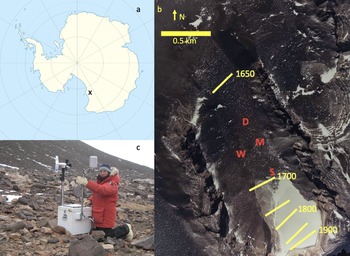


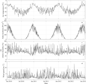


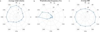

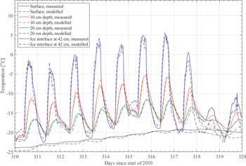


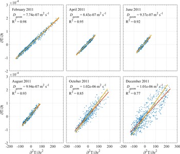
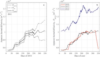


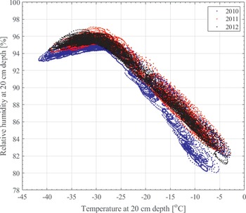
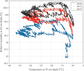


 Open access