2. Experimental data

We use the experimental data of Aussillous et al. (Reference Aussillous, Chauchat, Pailha, Médale and Guazzelli2013) who examined the mobile layer of a granular bed in laminar flows in a rectangular-channel flow. This database yields depth-resolved profiles of particle velocity for a range of fluid heights $h_f$ as the height of the clear-liquid layer above the granular bed and flow rates in the laminar regime.

We summarise below the main features of the experimental apparatus used to obtain this database. Further details can be found in Aussillous et al. (Reference Aussillous, Chauchat, Pailha, Médale and Guazzelli2013). Two batches of particles, consisting respectively of borosilicate spheres having a mean diameter $d_p=1.1\pm 0.1$ mm and a specific density $(\rho _p - \rho _f)/\rho _f=1.1$ and of polymethyl methacrylate (PMMA) spheres having a mean diameter $d_p=2.04\pm 0.03$ mm and a specific density $(\rho _p - \rho _f)/\rho _f=0.1$, were selected, where $\rho _f$ is the fluid density. The particles were immersed in a viscous fluid (mainly composed of Triton X-100 and water) having the same refractive index as the respective particles. A dye (Rhodamine 6G) that fluoresces when illuminated by the laser in the wavelength range greater than 555 nm was added to the fluid. The flow set-up consisted of a horizontal rectangular channel of length $L_x=100$ cm, height $L_y=6.5$ cm and width $L_z=3.5$ cm, where $x$, $y$ and $z$ denote the streamwise, vertical and spanwise coordinates, respectively. To create a sediment bed, the channel was filled up with monodisperse particles and fluid, then turned upside down and tilted to consolidate the sediment bed. Afterwards, the channel was set horizontally and flipped back to its original position and a pressure gradient was applied to generate a small flow rate. This procedure was applied to fill solely the channel entrance with sedimented particles, leaving an empty buffer space near the outlet of the channel. A constant fluid flow rate, $Q_f$, was then applied to erode the sedimented bed of particles into the empty buffer space. In this way, the fluid shear stress at the top of the bed decreased as the fluid–particle interface (upstream from the buffer region) receded (i.e. $h_f$ increased) with time. The fluid–sediment interface is detected by computing the maximum change of slope of the averaged grey level profile (green line in figure 1a,c). Several runs were conducted for each particle type, by varying the imposed flow rate. Data for the velocity profile (particle velocity, $u_p$ and fluid velocity, $u_f$, in solely the pure fluid zone for the PMMA particles) were collected by averaging 10 images over 0.5 s every 5 s. In addition, bulk quantities were deduced such as the time evolution of the particle bed height, $h_p$, and the flow rate per unit width, $q_{f,exp}$, by neglecting the role of the moving granular layer. The experiments were conducted in the viscous regime with a Reynolds number defined as ${{\textit {Re}}}=\rho _f Q_f / \eta _f L_z$ in the range $0.2 <{{\textit {Re}}} < 1.2$. The Stokes number based on the shear rate $\dot {\gamma }$ was $St = \rho _p d_p^{2} \dot {\gamma } / \eta _f \approx 0.01$ on average.

Figure 1. Depth-resolved quantities extracted from the experiments for (a,b) borosilicate particles with $Q_f=2.7\times 10^{-6} \ \textrm {m}^{3}\ \textrm {s}^{-1}$ and $h_f=6.3$ mm and for (c,d) PMMA particles with $Q_f=2.7\times 10^{-6}\ \textrm {m}^{3}\ \textrm {s}^{-1}$ and $h_f=15.3$ mm corresponding to runs 1 and 12 of Aussillous et al. (Reference Aussillous, Chauchat, Pailha, Médale and Guazzelli2013), respectively. (a,c) Averaged images over 10 s having a length scale (a) $0.029\ \textrm {mm}\ \textrm {pixel}^{-1}$ and (b) $0.046\ \textrm {mm}\ \textrm {pixel}^{-1}$ with the corresponding grey-level profile (green curve) and the linear adjustment in the pure fluid zone (yellow straight line). (b,d) Normalised volume-averaged velocity profile, $U/U_{max}$ (red $\circ$), and volume-fraction profile, $\phi /\phi _c$ (blue $\square$). The full line corresponds to the theoretical velocity profile in the pure fluid zone (2.3). The white and grey horizontal dashed lines in (a,c) and (b,d) respectively indicate the fluid–particle interface at $y = h_p$.

The most difficult quantity to extract from the experiments is the particle volume fraction, $\phi$. In Aussillous et al. (Reference Aussillous, Chauchat, Pailha, Médale and Guazzelli2013), the volume-fraction profile for the borosilicate particles was evaluated by using the averaged grey-level profile, $P_I(y)$, of the same images as those utilised to infer the velocity profile and by scaling it by the grey-level profile of the immobile initial bed, which is assumed to be at the constant maximum particle volume fraction $\phi _c= 0.585$. However, the laser intensity was likely to have changed during a run and the maximum packing in the bed measured with this method was found to vary with the fluid height. We thus decided to revisit these data and to consider another method (also based on the averaged grey-level profile) to evaluate the volume fraction. As in Aussillous et al. (Reference Aussillous, Chauchat, Pailha, Médale and Guazzelli2013), we suppose that the grey-level intensity gradient is mainly due to a linear broadening of the laser line due to the use of a laser line generator with a finite fan angle (Dijksman et al. Reference Dijksman, Rietz, Lőrincz, van Hecke and Losert2012). First, we adjust the intensity decay in the pure fluid zone by a linear function, $P_I=P_{0l}(1-y/y_0)$, where $P_{0l}$ and $y_0$ are constants which depend on the laser and the fluid properties, see figure 1(a,c) corresponding respectively to run 1 and run 12 of Aussillous et al. (Reference Aussillous, Chauchat, Pailha, Médale and Guazzelli2013). Second, for the liquid–particle mixture we assume that $P_I(y)=[(1-\phi ) P_{0l}+\phi P_{0s}](1-y/y_0)$ where $P_{0s}$ is related to the particle properties. We then introduce $A=P_I(y)/(1-y/y_0)$, which is averaged over the same box size as that used for the velocity profile. If we suppose that $\phi (h_c)=\phi _c$ and $A(h_c)=A_c$ at the bottom of the mobile granular layer $h_c$, i.e. the height for which particle motion ceases, the volume fraction is given by $\phi =\phi _c [A(y)-1]/(A_c-1)$. In figure 1(b,d), we have plotted the normalised volume fraction, $\phi /\phi _c$, vs the vertical position made dimensionless using the particle diameter, $y/d_p$, for (b) borosilicate particles ($Q_f=2.7\times 10^{-6}\ \textrm {m}^{3}\ \textrm {s}^{-1}$ and $h_f=6.3$ mm) and (d) PMMA particles ($Q_f=2.7\times 10^{-6}\ \textrm {m}^{3}\ \textrm {s}^{-1}$ and $h_f=15.3$ mm). We observe that the volume fraction increases rapidly downward from the fluid–particle interface and reaches quickly a constant value after approximately two sphere diameters.

To examine the rheological behaviour of the sheared sediment bed, we need to infer the depth-resolved shear rate, $\dot {\boldsymbol {\gamma }}$, the mixture shear stress, $\tau$, and the particle pressure, $p_p$, from the particle velocity profile, $u_p$, and the volume-fraction profile, $\phi$. First, we interpolate linearly the velocity and volume-fraction profiles to obtain their value at the fluid–bed interface, $u_{p,in}$ and $\phi _{in}$, see the red $x$ and blue $+$ on the dashed line in figure 1(b,d). The shear rate profile, $\dot {\boldsymbol {\gamma }}(y)=\textrm {d}u_p/{\textrm {d} y}$, is simply deduced numerically from the particle velocity profile using a second-order finite difference approximation. To evaluate the total shear stress and the particle pressure, we use the two-phase modelling developed in Aussillous et al. (Reference Aussillous, Chauchat, Pailha, Médale and Guazzelli2013). In this approach, a flat particle bed of thickness $h_p$ is subjected to a Poiseuille flow driven by a pressure gradient, $\partial p_f/\partial x$, in a horizontal channel. The flow is assumed to be two-dimensional, stationary and uniform in the streamwise direction, also parallel and laminar. From the fluid phase equation (i.e. the Brinkman equation), the volume-averaged velocity in the horizontal $x$-direction is found to be $U = \phi \, u_p + (1-\phi ) \, u_f\approx u_p\approx u_f$ in the bed due to the small permeability. In the laminar regime, the momentum equations for the mixture (particles plus fluid) then write

(2.1)$$\begin{gather} {\tau}({y})={\tau}_f({h}_p)-\frac{\partial p_f}{\partial{x}}({h}_p-{y}), \end{gather}$$

(2.2)$$\begin{gather}\frac{\partial p_p}{\partial y} =\phi(y) \Delta\rho g , \end{gather}$$

where $g$ is the gravitational acceleration and $\Delta \rho =\rho _p-\rho _f$ corresponds to the density difference between the two phases. To compute the particle pressure profile inside the bed, (2.2) is integrated numerically along the vertical $y$-direction. It shows that the pressure of the particle phase is proportional to the apparent weight of the solid phase and increases when penetrating inside the bed. The total stress profile inside the bed is deduced from (2.1), provided the stresses applied by the fluid at the fluid/bed interface, ${\tau }_f(h_p)$, and the imposed fluid pressure gradient, ${\partial {p}_f}/{\partial {x}}$, are given.

Due to the lack of measurements of the fluid velocity in the pure fluid zone for the borosilicate particles, we need to reconstruct the fluid velocity profile for this batch of spheres based on the following assumptions:

1. (i) The fluid velocity, $u_f$, is zero at the top wall ($y=L_y$) and matches the particle velocity, $u_{p,in}$, at the bed height ($y=h_p$).

2. (ii) The fluid velocity profile is parabolic for $y>h_p$ which yields the analytical solution for a mixed Couette–Poiseuille flow

   (2.3)\begin{equation} u_f = \frac{{\partial {p}_f}/{\partial{x}}}{2\eta_f}\left(y^{2}-L_y^{2}\right) - \left[\frac{u_{p,in}}{h_f} + \frac{{\partial {p}_f}/{\partial{x}}}{2\eta_f}\left(h_p + L_y\right)\right](y-L_y) , \end{equation}
   where $h_f = L_y - h_p$ is the height of the clear fluid layer.

3. (iii) The fluid flux, $q_{f,exp}$, is written as

   (2.4)\begin{equation} q_{f,exp} = \int_0^{h_p} (1-\phi) u_p \, \mathrm{d}y + \underbrace{\int_{h_p}^{L_y} u_f \, \mathrm{d}y}_{q_f} , \end{equation}
   considering that the fluid velocity matches the particle velocity inside the bed.

Using the experimental flow rate per unit width, $q_{f,exp}$, and the experimental vertical profiles of $\phi$ and $u_p$, the pure fluid flow rate $q_f$ is deduced from (2.4) by numerical integration and the pressure gradient for the parabolic velocity profile is then obtained as ${\partial {p}_f}/{\partial {x}} = ({6 \eta _f}/{h_f^{3}}) (h_f u_{p,in} - 2 q_f)$. Inserting this value in (2.3), we can calculate the fluid velocity profile in the pure fluid zone, see the black full curves in figure 1(b–d). The agreement with the experimental fluid velocity measurement for the PMMA particles is found to be good, see figure 1(d). This validates the present reconstruction method and its use for the borosilicate particles. Note that this method does not enforce a continuity of stress from the clear fluid phase to the particle phase; the obtained fluid and particle velocity profiles exhibit a change in slope at the fluid/bed interface. The fluid shear stress at the bed interface is then given by $\tau _f(h_p)= \frac {1}{2}({\partial {p}_f}/{\partial {x}})(L_y-h_p )- \eta _f u_{p,in}/h_f$ and the vertical profile of the shear rate is simply given by (2.1).

The extraction and reconstruction methods described above provide all the quantities needed to investigate the rheology of the mobile sediment bed: $\mu (J)$ and $\phi (J)$ or equivalently $\eta _s(\phi )$ and $\eta _n(\phi )$.

3. Simulation data

In the present work, we use the framework described in detail in Biegert et al. (Reference Biegert, Vowinckel and Meiburg2017a,Reference Biegert, Vowinckel, Ouillon and Meiburgb) to execute several simulations in an attempt to compare to the different experimental results of Aussillous et al. (Reference Aussillous, Chauchat, Pailha, Médale and Guazzelli2013) at different flow rates and fluid heights. In order to keep the paper self-contained, we provide a brief summary of the computational approach.

The particle-laden flows of interest require us to solve the Navier–Stokes equation

(3.1)\begin{equation} \rho_f \left[\frac{\partial{\boldsymbol{u}_f}}{\partial{t}}+\boldsymbol{\nabla}\boldsymbol{\cdot}(\boldsymbol{u}_f\boldsymbol{u}_f)\right] = \boldsymbol{\nabla} \boldsymbol{\tau}_f + \boldsymbol{f}_b + \boldsymbol{f}_{IBM}, \end{equation}

where $\boldsymbol {u}_f=(u_f,v_f,w_f)^\textrm {T}$ denotes the fluid velocity vector and $t$ time. The fluid stress tensor is given by $\boldsymbol {\tau }_f = -p_f \boldsymbol {E} + \eta _f [\boldsymbol {\nabla } \boldsymbol {u}_f + (\boldsymbol {\nabla } \boldsymbol {u}_f)^\textrm {T}]$, where $p_f$ represents the fluid pressure with the hydrostatic component subtracted out and $\boldsymbol {E}$ the identity matrix. The right-hand side includes the volume forces $\boldsymbol {f}_b=(\,f_{b,x},0,0)^\textrm {T}$ and $\boldsymbol {f}_{IBM}$. The former is a source term used to create the pressure gradient driving the flow and the latter an immersed boundary force used to enforce the no-slip condition on the particle surface. We discretise the equations of motion for the fluid on a cubic finite difference mesh ($\lambda = \Delta x = \Delta y = \Delta z$).

The numerical treatment is based on the IBM for fluid–particle coupling (Uhlmann Reference Uhlmann2005; Kempe & Fröhlich Reference Kempe and Fröhlich2012a) and the scheme of Biegert et al. (Reference Biegert, Vowinckel and Meiburg2017a) for particle–particle interaction.

We solve for the translational velocity, $\boldsymbol {u}_p$,

(3.2)\begin{equation} m_p\, \frac{\text{d}\boldsymbol{u}_p}{\text{d} t} = \underbrace{\oint_{\varGamma_p} \boldsymbol{\tau}_f \boldsymbol{\cdot} \boldsymbol{n}\, {\text{d}A}}_{=\boldsymbol{F}_{h,p}} + \underbrace{V_p\,(\rho_p-\rho_f )\, \boldsymbol{g}}_{=\boldsymbol{F}_{g,p}} + \boldsymbol{F}_{i,p} , \end{equation}

and the angular velocity, $\boldsymbol {\omega }_p$,

(3.3)\begin{equation} I_p \,\frac{ \text{d}\boldsymbol{\omega}_p}{\text{d} t} = \underbrace{\oint_{\varGamma_p} \boldsymbol{r}_p\times(\boldsymbol{\tau}_f\boldsymbol{\cdot}\boldsymbol{n})\,{\text{d}A}}_{=\boldsymbol{T}_{h,p}} + \boldsymbol{T}_{i,p} , \end{equation}

of spherical particles, where $m_p$ is the particle mass, $I_p$ the particle moment of inertia, $V_p$ the particle volume and $\boldsymbol {g}=(0, -g, 0)^\textrm {T}$ the gravitational acceleration vector. The fluid acts on the particles through the hydrodynamic stress tensor $\boldsymbol {\tau }_f$, where $\boldsymbol {r}_p$ represents the vector from the particle centre to a point on the surface $\varGamma _p$ and $\boldsymbol {n}$ is the unit normal vector pointing outwards from that point. The net force and torque acting on the particle centre of mass due to particle interactions are given by $\boldsymbol {F}_{i,p}$ and $\boldsymbol {T}_{i,p}$, respectively.

We evaluate the particle interaction forces and torques according to Biegert et al. (Reference Biegert, Vowinckel and Meiburg2017a). The resulting collision model involves normal contact forces, $\boldsymbol {F}_{n}$, tangential (frictional) contact forces, $\boldsymbol {F}_{t}$, and short-range hydrodynamic lubrication forces, $\boldsymbol {F}_{l}$, to provide the total collision force

(3.4)\begin{equation} \boldsymbol{F}_{i,p} = \sum_{q,\,q \neq p}^{N_{tot}} \left( \boldsymbol{F}_{l,pq} + \boldsymbol{F}_{n,pq} + \boldsymbol{F}_{t,pq}\right) , \end{equation}

where $N_{tot}$ is the total number of particles and the subscript $pq$ indicates interactions of particle $p$ with particle $q$. According to Cox & Brenner (Reference Cox and Brenner1967), we model the unresolved hydrodynamic component of the lubrication forces in our simulations as

(3.5)\begin{equation} \boldsymbol{F}_{l,pq} = \begin{cases} - \dfrac{6 {\rm \pi}\eta_f R_{eff}^{2}}{\max(\zeta_n,\zeta_{min})} \boldsymbol{g}_n & 0 < \zeta_n \leqslant 2h \\ 0 & \text{otherwise} \end{cases} \end{equation}

where $\zeta _n$ is the gap size, $R_{eff}=R_p R_q/(R_p + R_q)$ the effective radius and $R_p$ and $R_q$ are the radii of the two interacting particles. Furthermore, $\zeta _{min}=3\times 10^{-3}R_p$ is a limiter as calibrated by Biegert et al. (Reference Biegert, Vowinckel and Meiburg2017a) that can be interpreted as the roughness of the particle surface and $\boldsymbol {g}_n$ is the normal component of the relative velocity of the two colliding particles. The repulsive normal component is represented by a nonlinear spring-dashpot model for the normal direction

(3.6)\begin{equation} \boldsymbol{F}_{n,pq} ={-}k_n |\zeta_n|^{3/2} \boldsymbol{n} - d_n \boldsymbol{g}_{n} , \end{equation}

where $k_n$ and $d_n$ represent stiffness and damping coefficients that are adaptively calibrated for every collision/contact to prescribe a restitution coefficient of ${e_{dry}=-u_{o}/u_{i}=0.97}$ (Kempe & Fröhlich Reference Kempe and Fröhlich2012b). Here, $u_{o}$ and $u_{i}$ indicate the normal components of the relative particle speed immediately after and right before the particle contact, i.e. $\zeta _n=0$. The forces in the tangential direction are modelled by a linear spring-dashpot system capped by the Coulomb friction law as

(3.7)\begin{equation} \boldsymbol{F}_{t,pq} = \min \left({-}k_t \boldsymbol{\zeta}_t - d_t \boldsymbol{g}_{t,cp} , ||\mu_f \boldsymbol{F}_n|| \boldsymbol{t} \right) , \end{equation}

where $k_t$ and $d_t$ are stiffness and damping computed according to Thornton, Cummins & Cleary (Reference Thornton, Cummins and Cleary2011) and Thornton, Cummins & Cleary (Reference Thornton, Cummins and Cleary2013), $\mu _f=0.15$ represents the friction coefficient between the two surfaces, $\boldsymbol {\zeta }_t$ is the tangential displacement integrated over the time interval for which the two particles are in contact (Thornton et al. Reference Thornton, Cummins and Cleary2013) and $\boldsymbol {t}$ is a unit vector pointing into the tangential direction. The empirical parameters $e_{dry}=0.97$ and $\mu _f=0.15$ have been taken from experiments involving glass spheres (Gondret, Lance & Petit Reference Gondret, Lance and Petit2002; Joseph & Hunt Reference Joseph and Hunt2004). Using these values, the contact model has been validated in detail by Biegert et al. (Reference Biegert, Vowinckel and Meiburg2017a) against seminal experimental benchmark data involving the same material (Foerster et al. Reference Foerster, Louge, Chang and Allia1994; Gondret et al. Reference Gondret, Lance and Petit2002; Ten Cate et al. Reference Ten Cate, Derksen, Portela and Van Den Akker2004; Aussillous et al. Reference Aussillous, Chauchat, Pailha, Médale and Guazzelli2013). Note that these parameters were not measured for the particles used in the experiments of Aussillous et al. (Reference Aussillous, Chauchat, Pailha, Médale and Guazzelli2013) and may, hence, be different.

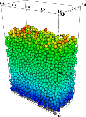
In the present work, we consider a computational set-up very similar to the one presented in Aussillous et al. (Reference Aussillous, Chauchat, Pailha, Médale and Guazzelli2013) (figure 2a). The domain has dimensions ${L_x \times L_y \times L_z = 20d_p \times 30d_p \times 10d_p}$. We discretise the domain with a regular grid that is equidistant in all three directions and has a resolution of 25.6 grid cells per particle diameter, which is a fine enough resolution to obtain results independent of the grid cell size, as shown by Biegert et al. (Reference Biegert, Vowinckel, Hua and Meiburg2018). We generate the bed by allowing 4339 monodisperse particles to settle under gravity, without the influence of the surrounding fluid, onto a layer of 200 fixed particles whose centres randomly vary in height above the bottom wall within a range of $d_p$, providing an irregular roughness (Jain, Vowinckel & Frhlich Reference Jain, Vowinckel and Fröhlich2017). The resulting bed fills the domain to approximately a height of $h_p \approx 20d_p$ from the bottom wall, where $h_p$ is the particle bed height, leaving a gap of approximately $10d_p$ between the top wall and the top of the particle bed. For the simulation runs, we use a particle density $\rho _p/\rho _f=2.1$ and a Galileo number of $Ga=0.85$. A definition of $Ga$ as well as a summary of the relevant simulation parameters is given in table 1. We employ a predefined Poiseuille flow in the clear fluid region above the sediment bed as a reference case for the simulation. For this reference case, we define the reference length $y_{ref} = 10d_p = L_y/3$, the reference velocity of $u_{ref} = -y_{ref}^{2} \,f_{b,x} / (12 \eta _f)$ and the reference stress $\sigma _{ref} = -y_{ref} \,f_{b,x} /2$ to compute the corresponding Reynolds and Shields numbers (cf. table 2).

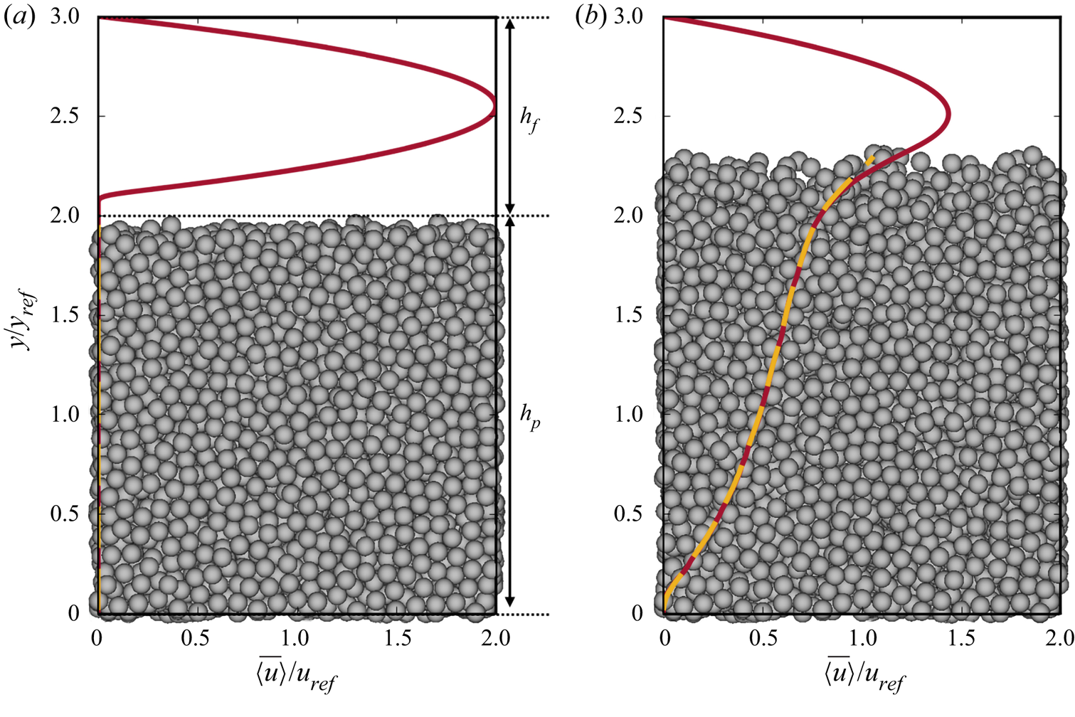
Figure 2. (a) Initial conditions for fluid velocity and bed configuration at $t/t_{base}=0$ and (b) fully developed state at $t/t_{base}=10$ for simulation Re67 as listed in table 2. Lines indicate the average streamwise ($x$-direction) fluid velocity (dark grey, red online) and particle velocity (light grey, yellow online), where the consecutive averaging in the horizontal plane and time is defined by (3.9).

Table 1. Simulation parameters for the pressure-driven flow over a bed of particles. CFL, Courant–Friedrichs–Lewy.

Table 2. Simulation parameters for different runs of the pressure-driven flow over a bed of particles. The Reynolds and Shields numbers based on the reference case (predefined Poiseuille flow above the sediment bed), i.e. $Re_{ref} = \rho _f u_{ref} y_{ref} / \eta _f$ and 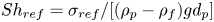$Sh_{ref} = \sigma _{ref}/[(\rho _p-\rho _f) g d_p]$, respectively. The individual simulation is run for the duration $t_{sim}$, and the momentum balance is analysed by using time-averaged data over the interval $t_{avg}$.

We enforce different volumetric flow rates, governed by the volume force $\,f_{b,x}$. As it can take a long time for a simulation to reach a statistically steady state when initialised from rest, we found it to be more efficient to obtain a steady state by initialising the flow with a large pressure gradient that mobilises the entire bed (run Re67 in figure 3(a) and table 2). To allow for a direct comparison among the different runs, we therefore define $u_{base}=u_{ref} (\text {Re67})$, $t_{base} = y_{ref} / (1.5 u_{base})$ and $\sigma _{base} = \sigma _{ref}(\text {Re67})$. By the end of the simulation Re67, the bed has dilated to a height of $h_p/y_{ref} \approx 2.3$ (figure 3b), and the particles just above the fixed layer at the bottom of the domain are moving (figure 2b). After this initialisation phase, the imposed pressure gradient is reduced to produce simulations Re17 and Re33. Re8 is carried out by continuing Re17 with an even lower imposed pressure gradient. This procedure allows us to quickly reach a steady state for runs Re17 and Re8, as can be seen in figure 3(a), whereas Re33 is still in the process of dilation.

Figure 3. Sheared particle bed. (a) Particle volumetric flux $q_p = ({1}/{L_x \, L_z} )\sum _{p=1}^{N_{tot}} V_p u_{p,x}$, for the different simulation runs. Dotted lines indicate the average particle flux over the averaging time interval for each simulation. (b) Bed height, defined at $\left \langle \phi \right \rangle = 0.05$.

To compare the simulation results to rheological models, we have to analyse the discrete information of the particle phase in our simulations, such as particle velocities and forces, from a continuum viewpoint. To this end, we employ the coarse-graining method (CGM) based on the works of Goldhirsch (Reference Goldhirsch2010) and Weinhart et al. (Reference Weinhart, Thornton, Luding and Bokhove2012). This CGM conserves quantities of interest, but additionally smooths out the resulting continuum field. For a given discrete particle quantity $\theta _p$, we define its coarse-grained continuous counterpart, $\theta ^{cg}$, as

(3.8)\begin{equation} \theta^{cg}(\boldsymbol{x},t) = \sum_{p=1}^{N_{tot}} \theta_p \mathcal{W}(\boldsymbol{x} - \boldsymbol{x}_p(t)) , \end{equation}

where $\boldsymbol {x}_p(t)$ is the position of the centre of particle $p$, and $\mathcal {W}(\boldsymbol {r})$ is the conservative coarse-graining function that smears a given local quantity in a spherical volume of radius $|\boldsymbol {r}|$. The main property is that $\int _{\mathbb {R}^{3}} \mathcal {W}(\boldsymbol {r}) \, \text {d}\boldsymbol {r} = 1$. We implemented a coarse-graining function based on the Dirac delta function of Roma, Peskin & Berger (Reference Roma, Peskin and Berger1999), which is the same delta function used in the IBM (Uhlmann Reference Uhlmann2005). The filter $|\boldsymbol {r}|$ has to be as small as possible to fully exploit the highly resolved simulation data for our rheological analysis, but large enough to smooth out the sub-particle scale. Here, we choose $\lvert \boldsymbol {r}\rvert = 1.5 d_p$, which was deemed to be a good compromise to satisfy these requirements.

The steady-state configuration for the moving bed is steady only in a time-averaged sense, because particle collisions and positions continuously fluctuate. We therefore define the time average of a given continuous field $\theta$ to be

(3.9)\begin{equation} \overline{\left\langle \theta\right\rangle}(y) = \frac{1}{t_{avg,2}-t_{avg,1}} \int_{t_{avg,1}}^{t_{avg,2}}\frac{1}{L_x L_z} \int_0^{L_z} \int_0^{L_x} \theta(x,y,z,t) \, \mathrm{d}\kern0.7pt x \, \mathrm{d}z \, \mathrm{d}t , \end{equation}

where the overbar and angular brackets represent averaging in time and space, respectively (Vowinckel, Kempe & Fröhlich Reference Vowinckel, Kempe and Fröhlich2014; Vowinckel et al. Reference Vowinckel, Nikora, Kempe and Fröhlich2017a,Reference Vowinckel, Nikora, Kempe and Fröhlichb). Note that this averaging operator applies for both continuous fluid quantities and coarse-grained particle quantities. We present the values for $t_{avg,1}$ and $t_{avg,2}$ in table 2. These time-averaging windows were chosen to capture the steady-state results, or as large a time span as possible for as similar a particle flux as possible (figure 3). We will show, however, that our results for the rheology are independent of transient behaviour for all Reynolds numbers investigated.

We can use (3.8) to obtain a continuous field of $\phi$ and (3.9) to generate vertical profiles of $\overline {\left \langle \phi \right \rangle }$ and $\overline {\left \langle u_f\right \rangle }$ by computing double-averaged values (in space and time, cf. figure 4). For the analysis of the rheology, we exclude values for $y/y_{ref}<0.68$ to eliminate boundary effects from the artificial bed roughness at the bottom wall. We observe the same evolution for the volume fraction as in the experiments with a rapid increase downward from the fluid–particle interface to reach a constant value after a few sphere diameters. Here, we follow the definition of Biegert et al. (Reference Biegert, Vowinckel and Meiburg2017a) to determine the fluid–sediment interface at $\overline {\left \langle \phi \right \rangle }=0.05$. The oscillations of $\overline {\left \langle \phi \right \rangle }$ in this region reflect the sub-particle scale as the particle are layered within the sediment bed (figure 4a). We therefore apply the coarse-graining radius of $|\boldsymbol {r}|= 1.5 d_p$ to the grid resolved data shown in this figure to smooth out the layered structure in these vertical profiles. Note that figure 4(b) yields $\dot {\gamma }=\partial \overline {\left \langle u_f\right \rangle }/\partial y$ as another rheological quantity. Looking at the double-averaged fluid velocity profiles in figure 4(b), the three cases represent three distinctively different regimes (Jenkins & Larcher Reference Jenkins and Larcher2017). The sediment bed of Re8 reaches a quasi-static regime of the granular suspension, whereas the sediment motion in Re17 and Re33 can be considered ‘layered’ and ‘collisional’, respectively. There is a clear qualitative difference between run Re8, whose velocity profile is concave and goes to zero within the bed at $y/y_{ref} \approx 0.5$, and run Re33, whose velocity profile is convex, goes to zero only at the fixed particles at the lower wall. Note that the fluid velocity is to a good approximation equal to the particle velocity, which is consistent with the observation of Aussillous et al. (Reference Aussillous, Chauchat, Pailha, Médale and Guazzelli2013). The Stokes number is in the range $0.19\leqslant St\leqslant 0.77$, which is 20 to 80 times larger than the values obtained from the experimental data § 2, but still expected to be in the viscous regime (Ness & Sun Reference Ness and Sun2015).

Figure 4. Sheared particle bed: profiles for the different simulation runs averaged horizontally and in time for (a) the particle volume fraction and (b) the streamwise velocity. The average fluid velocity (solid coloured lines) is given by (3.9), while the average coarse-grained particle velocity (circles) is given by (3.8).

While we can readily extract the quantities for $\phi$ and $\dot {\boldsymbol {\gamma }}$ from figure 4, an additional investigation of the total stress balance of the fluid–particle mixture in $x$- and $y$-directions is needed to compute the total shear stress $\tau$ and the granular pressure $p_p$ as will be detailed in the next section.

4. Stress balance of the simulation data

This section presents the analysis of the stress balance for the fluid–particle mixture to compute wall-normal profiles of the rheological quantities $\tau$ and $p_p$. To this end, we follow the argument of the previous numerical work (Biegert Reference Biegert2018; Biegert et al. Reference Biegert, Vowinckel, Hua and Meiburg2018; Vowinckel et al. Reference Vowinckel, Biegert, Luzzatto-Fegiz and Meiburg2019), where the full derivation of the stress balances in both shearing ($x$) and wall-normal ($y$) directions is given from first principles. In addition, a detailed analysis of the present data sets for all components entering the stress balances in the shear and wall-normal directions can be found in Biegert (Reference Biegert2018).

4.1. Stress balance in the $x$-direction to obtain the total stress

To obtain the total shear stress, we consider the momentum balance of the fluid phase, i.e. the Navier–Stokes equations (3.1), over the control volume $\varOmega _{CV}$ in the $x$-direction spanning from the top wall $\varGamma _w$ to some arbitrary height $y$ with the lower boundary being $\varGamma _y$ and involving multiple particles (figure 5). We distinguish the free fluid from the particle interior as exemplified in figure 5 using $\varOmega _{CV}^{+}$ and $\varGamma _y^{+}$ for parts of the domain that are occupied by fluid and the lower boundary, respectively.

Figure 5. Shaded control volume for the averaging involving multiple particles. All of the volumes and surfaces required for (4.1) are indicated.

We can simplify the momentum balance of the fluid phase for the following reasons. Owing to the periodic boundary conditions and the fact that we impose the Poiseuille flow via the volume force $\boldsymbol {f}_b$, the pressure term ($\partial p_f / \partial x$ in (3.1)) does not contribute to the $x$-momentum, since our control volume covers the entire streamwise extent of the domain. At the top wall $\varGamma _w$, the vertical velocity, $v_f$, is zero, so that only $\eta _f \partial u_f/\partial y$ contributes to the fluid stress. At the lower boundary, $\varGamma _y$, the pressure again does not play a role and the convective term vanishes due to the laminar flow conditions, so that the long-range hydrodynamic stress originates from the viscous term. Finally, we include $\,f_{IBM,x}$ as the sum of all hydrodynamic stresses arising from pressure and viscous forces that act on the particle surfaces $L_{CV}$ enclosed in $\varOmega _{CV}$. These assumptions yield

(4.1) \begin{align} \underbrace{\int_{\varGamma_w} \eta_f \frac{\partial u_f}{\partial y} \,\mathrm{d}A + \int_{\varOmega_\mathit{CV}} \,f_{b,x} \,\mathrm{d}V}_{{External\ force}} &= \underbrace{\int_{\varGamma_y^{+}} \eta_f \left(\frac{\partial u_f}{\partial y} + \frac{\partial v_f}{\partial x}\right) \,\mathrm{d}A }_{{Fluid\ force}}\nonumber\\ &\quad \underbrace{-\int_{L_{CV}} \,f_{{IBM,x}}\, {\mathrm{d}V} }_{{Particle\ force}}. \end{align}

The last term Particle force provides the linkage to the momentum balance of the particle phase, which can be obtained by applying the CGM (3.8) to the particle equation of motion (3.2). This yields

(4.2)\begin{equation} \boldsymbol{a}^{cg} = \boldsymbol{F}_h^{cg} + \boldsymbol{F}_g^{cg} + \boldsymbol{F}_i^{cg} , \end{equation}

where $\boldsymbol {a}^{cg}$, $\boldsymbol {F}_h^{cg}$, $\boldsymbol {F}_{g}^{cg}$ and $\boldsymbol {F}_{i}^{cg}$ are the coarse-grained forces due to the particle acceleration, hydrodynamic stress due to the IBM, gravity and particle interactions, respectively. Similar to the fluid momentum balance, we can analyse the coarse-grained particle forces within a control volume spanning the entire domain in the streamwise and spanwise directions and extending from the top wall to an arbitrary height $y$. Integrating (4.2) over this volume, we obtain

(4.3)\begin{equation} \int_{\varOmega_\mathit{CV}} \boldsymbol{a}^{cg} \,\mathrm{d}V = \int_{\varOmega_\mathit{CV}} \left(\boldsymbol{F}_h^{cg} + \boldsymbol{F}_g^{cg} + \boldsymbol{F}_i^{cg} \right) \mathrm{d}V . \end{equation}

If particles are in a steady state, either naturally or through double averaging, then the acceleration term vanishes. Furthermore, our set-up of a horizontal channel yields $F_{g,x}=0$. We can, therefore, use the fact that $\,f_{IBM,x}=F_{h,x}^{cg}=-F_{i,x}^{cg}$ and apply (3.4) to further distinguish between normal and tangential forces due to particle contact and friction ($F_{n,x}^{cg}$ and $F_{t,x}^{cg}$) and short-range hydrodynamic lubrication forces ($F_{l,x}^{cg}$).

Using the averaging operator (3.9) and dividing by the horizontal area of the domain, we can rewrite (4.1) as

(4.4) \begin{align} \underbrace{\eta_f \overline{\left\langle\left.\frac{\partial u_f}{\partial y}\right|_{L_y}\right\rangle} + \bar{f}_{b,x} (L_y - y)}_{{External/total\ stress}}& = \underbrace{\eta_f \overline{\left\langle\gamma\left.\left(\frac{\partial u_f}{\partial y} + \frac{\partial v_f}{\partial x} \right)\right|_y \right\rangle} -\int_y^{L_y} \overline{\left\langle F_{l,x}^{cg}\right\rangle} \,\mathrm{d}y }_{{Hydrodynamic\ stress}}\nonumber\\ &\quad \underbrace{+\,\int_y^{L_y} \left(\overline{\left\langle F_{{n,x}}\right\rangle}+ \overline{\left\langle F_{{t,x}}\right\rangle}\right) {\mathrm{d}y} }_{{Contact\ stress}}, \end{align}

where $\gamma$ is an indicator function for the fluid ($\gamma = 1$ outside the particle and $\gamma = 0$ inside the particle), resulting in double-averaged equations for laminar flows akin to Nikora et al. (Reference Nikora, Ballio, Coleman and Pokrajac2013) and Vowinckel et al. (Reference Vowinckel, Nikora, Kempe and Fröhlich2017a,Reference Vowinckel, Nikora, Kempe and Fröhlichb). We have also used the fact that $\eta _f$, $\rho _f$ and $\,f_{b,x}$ are constant throughout the domain. It is important to note that we are explicitly separating the stresses arising from hydrodynamic interactions and particle contacts, respectively (Gallier et al. Reference Gallier, Lemaire, Lobry and Peters2014; Gallier, Peters & Lobry Reference Gallier, Peters and Lobry2018), which will be analysed in more detail in § 5. The right-hand side of (4.4) comprises the long-range fluid stress due to viscous effects evaluated at height $y$ at the boundaries of the control volumes $\varGamma ^{+}_{CV}$ occupied by fluid as well as the short-range lubrication effects within the control volume $\varGamma ^{+}_{CV}$. The contact stress comprises both, normal contact forces and tangential frictional forces. Note that it was shown in Biegert et al. (Reference Biegert, Vowinckel, Hua and Meiburg2018) and Biegert (Reference Biegert2018) that there is also a viscous and convective stress inside the particles $\varGamma ^{-}_{CV}$ as a by-product of the IBM. For the present study, this effect does not contribute a significant part to the total stress balance. The external stress on the left-hand side of (4.4) consists of the viscous stress at the top wall and the stress from the body force acting throughout the control volume. It is also equal to all other stresses arising from the movement of the fluid and particles and is hence equivalent to the total stress $\tau _f$ needed to compute the rheological quantities $\mu (J)$ and $\eta _s$.

For the analysis of the stress balance of the fluid phase, we focus on runs Re8 and Re33 to get a sense of the results for different flow conditions. Figure 6 shows the momentum balance of the fluid phase, given by (4.4), for runs Re8 (figure 6a) and Re33 (figure 6b), in which we expect the external stress to match the sum of the hydrodynamic and contact stresses. As expected, the external stress at the top wall is close to $\overline {\left \langle \sigma _x\right \rangle }/\sigma _{ref}=-1$. In the upper part of the flow ($y/y_{ref} > 2.15$ and $y/y_{ref} > 2.3$ for Re8 and Re33, respectively), there are no particles, and the hydrodynamic stress matches all of the external stress. Within the particle bed ($y/y_{ref} < 2.3$), however, the majority of the external stress is taken up by particle contact. The total stress comes out to be a linear profile. Hence, the present results support the conceptual model (2.1) proposed by Aussillous et al. (Reference Aussillous, Chauchat, Pailha, Médale and Guazzelli2013) (figure 4(b) in this reference) and we can use these data to compute $\eta _s$ and $\mu$ in the following.

Figure 6. Stress balance of the fluid phase in the $x$-direction for a sheared particle bed according to (4.4). (a) run Re8 and (b) run Re33. The horizontal dashed line marks the height of the particle bed, $h_p$. As shown in (a,b), the sum of the hydrodynamic and contact stresses is in equilibrium with the external stress and consists mostly of the contact stress within the bed and the hydrodynamic stress above the bed.

Naturally, the hydrodynamic stress of the laminar flow is entirely made up of the viscous term alone. Run Re8 differs from Re33 in that the hydrodynamic stress reaches a higher positive value above the particle bed and quickly drops to zero within the particle bed. The hydrodynamic stress for Re33, on the other hand, increases with increasing depth within the particle bed. Since the entire sediment bed is set in motion for this case, the lubrication component makes a significant contribution to the hydrodynamic stress. These results are consistent with the velocity profiles in figure 4(b), where the concavity of the profile for Re8 results in a high shear stress at the fluid/particle bed interface and low stresses within the bed, while the convexity of the profile for Re33 leads to a large shear stress at the lower wall. The total stress, on the other hand, is completely dominated by particle contact within the sediment bed. This result is consistent with the locations of the sharp gradients in the stress balance, so that the hydrodynamic and contact stresses together close the $x$-momentum balance. It also shows that effects from the local acceleration term are negligible and that the unsteady flow conditions (figure 3) are expected to have no impact on the reported results even for cases of dilating and consolidating sediment beds (e.g. Re33).

4.2. Stress balance in the $y$-direction to obtain particle pressure

The rheological quantities $\eta _n$ and $\mu (J)$ require information about the particle pressure $p_p$, which we can obtain by further analysing the particle phase. Another way to interpret the bed particle pressure $p_p$ is to think of it as the total submerged weight of the particles (Vowinckel et al. Reference Vowinckel, Biegert, Luzzatto-Fegiz and Meiburg2019). Indeed, this has been done by Stickel & Powell (Reference Stickel and Powell2005) and Ouriemi et al. (Reference Ouriemi, Aussillous and Guazzelli2009) for continuum modelling. We can demonstrate the validity of this reasoning by analysing the momentum balance for the particle phase in the $y$-direction. To this end, we utilise the coarse-grained momentum balance of the particle phase (4.2) and apply the averaging operator (3.9) to recast (4.3) as a line integral in the wall-normal direction

(4.5)\begin{equation} \int_y^{L_y} \overline{\left\langle\boldsymbol{a}^{cg}\right\rangle} \,\mathrm{d}y = \int_y^{L_y} \left(\overline{\left\langle\boldsymbol{F}_h^{cg}\right\rangle} + \overline{\left\langle\boldsymbol{F}_g^{cg}\right\rangle} + \overline{\left\langle\boldsymbol{F}_i^{cg}\right\rangle}\right) \mathrm{d}y . \end{equation}

Since we are interested in the granular pressure, i.e. the bed weight, we consider only the vertical $y$-component. We again neglect the acceleration term, but keep the gravity term that is acting in the same vertical direction. Furthermore, we subdivide $\boldsymbol {F}_i^{cg}$ into the short-range hydrodynamic lubrication and particle contact component, $\boldsymbol {F}_l^{cg}$ and $\boldsymbol {F}_n^{cg}$ and $\boldsymbol {F}_t^{cg}$, respectively,

(4.6) \begin{align} \underbrace{-\int_y^{L_y} \overline{\left\langle F_{g,y}^{cg}\right\rangle} \,\mathrm{d}y}_{{Bed\ weight}} &= \underbrace{\int_y^{L_y} \overline{\left\langle F_{h,y}^{cg}\right\rangle} \,\mathrm{d}y+ \int_y^{L_y} \overline{\left\langle F_{l,y}^{cg}\right\rangle} \,\mathrm{d}y}_{{Hydrodynamic\ stress}}\nonumber\\ &\quad + \underbrace{\int_y^{L_y} \overline{\left\langle F_{n,y}^{cg}\right\rangle} \,\mathrm{d}y+\int_y^{L_y} \overline{\left\langle F_{t,y}^{cg}\right\rangle} \,\mathrm{d}y}_{{Contact\ stress}}. \end{align}

Since $\boldsymbol {F}_{g,p}= V_p(\rho _p-\rho _f)\boldsymbol {g}$, coarse graining the particle weight yields the left-hand side as the submerged bed weight, which is equivalent to the particle pressure

(4.7)\begin{equation} p_p = (\rho_p - \rho_f) \lvert \boldsymbol{g} \rvert \int_y^{L_y} \overline{\left\langle \phi \right\rangle} \, \mathrm{d}y . \end{equation}

We also note that (4.7) is the integral of (2.2), so that the present derivation provides a direct linkage to the two-phase modelling of Aussillous et al. (Reference Aussillous, Chauchat, Pailha, Médale and Guazzelli2013). Owing to the fact that we obtain full information of the solid volume fraction (cf. figure 4b), we do not need to introduce an artificial pressure at the fluid sediment interface. This was suggested by Houssais et al. (Reference Houssais, Ortiz, Durian and Jerolmack2016) (called $P_0$ in that study), but using such an artificial pressure would neither be in line with the two-phase modelling, nor would it obey the definition of our control volume sketched in figure 5. Hence, omitting $P_0$ naturally yields $J\rightarrow \infty$ for $\phi \rightarrow 0$, because $p_p\rightarrow 0$. This behaviour is consistent with the approach of Boyer et al. (Reference Boyer, Guazzelli and Pouliquen2011).

Figure 7 shows the coarse-grained particle phase stresses, given by the time average of (4.6) for runs Re8 (a) and Re33 (b). In figures 7(a) and 7(b), the bed weight increases almost linearly from the top of the particle bed down to the lower wall, balanced by the sum of the hydrodynamic and collision stresses. Again, this observation confirms the conceptual model of (2.2) of Aussillous et al. (Reference Aussillous, Chauchat, Pailha, Médale and Guazzelli2013). The fact that we have found a linear profile for this physical quantity simplifies the situation from a modelling perspective, i.e. one needs the sediment height and the total submerged weight of the sediment bed to reconstruct depth-resolved profiles of $p_p$. The results for the stress balance in $y$-direction show clear differences between runs Re8 and Re33. Owing to the normalisation, the dimensionless $y$-momentum collision stress is three times larger for Re8 than for Re33. Moreover, the hydrodynamic stress is positive for Re8 and negative for Re33, so that the collision stresses are less than and greater than the bed weight, respectively, for the stress balance to be in equilibrium. These deviations from zero stem from the fact that Re8 and Re33 are in the process of consolidation and dilation, respectively.

Figure 7. Stress balance of the particle phase in the $y$-direction for sheared particle beds according to (4.6). (a) run Re8 and (b) run Re33. The horizontal dashed line marks the height of the particle bed, $h_p$. Panels (a,b) show that the sum of the hydrodynamic and contact stresses is in equilibrium with the bed weight, i.e. $p_p$, with most of the weight supported by the contact stress. The hydrodynamic lift force acting on the particles can be (a) positive or (b) negative.

5. Rheology

We now turn to the examination of the rheological quantities extracted from the experimental measurements in § 2 and from the numerical simulations in §§ 3 and 4. We display these data within the pressure-imposed view by plotting the effective friction coefficient, $\mu =\tau /p_p$, and the bulk volume fraction, $\phi$, as a function of the viscous number, $J=\eta _f \dot {\gamma }/p_p$, in figure 8. The macroscopic friction coefficient, $\mu$, is found to be an increasing function of the viscous number, $J$, whereas the volume fraction, $\phi$, is a decreasing function of the viscous number, $J$, for both the experimental data coming from the two batches of spheres made of borosilicate ($+$) and PMMA ($\times$), where no appreciable differences can be seen between the runs of these two particle materials, and the numerical data coming from the three different runs at different Reynolds numbers.

Figure 8. (a) Effective friction coefficient, $\mu =\tau /p_p$, and (b) bulk volume fraction, $\phi$, vs the viscous number, $J=\eta _f \dot {\gamma }/p_p$. The solid lines are the asymptotic linear regressions in $\sqrt {J}$ (blue for the experiments and green for the simulations).

It is important to note, however, that figure 8 is not meant as a validation of the numerical results by comparing it to the post-processed experimental data of Aussillous et al. (Reference Aussillous, Chauchat, Pailha, Médale and Guazzelli2013) for the following reasons. First, the two data sets represent different conditions. The particle properties $e_{dry}$ and $\mu _f$ chosen for the simulations may not correspond to the (unknown) values of the experiments and the flow conditions expressed by the Stokes number differ by more than one order of magnitude. Second, owing to the difficulty in capturing experimentally the sediment transport layer close to the bed interface of only a few particle diameters thickness, the experimental data present significant scatter. Finally, recall that our data processing in § 2 assumes $u_f=u_{p,in}$ to reconstruct the experimental velocity profile, which slightly underestimates the fluid velocity in the sediment transport layer. On a similar note, the averaging operator using coarse-grained quantities (3.8) for the simulations yields an averaging window of three diameters in height to smooth out the sub-particle scale. For all these reasons, we can observe a rather large discrepancy between the experimental and numerical data for large $J$, i.e. in the sediment transport layer, but the qualitative trend is correctly reproduced.

Despite the discrepancy at large $J$, both data sets show asymptotic behaviour for small $J$ in figure 8(b). The results can therefore be used to deduce the critical parameters $\mu _c$ and $\phi _c$ and provide proper scaling for our rheological analysis. Among the numerical results, only the data for the smallest Reynolds number (run Re8) reach the limit of small $J$, i.e. $J<10^{-2}$ and, hence, small $\dot {\gamma }$. The data coming from run Re8 and from the experiments show that both $\phi$ and $\mu$ tend to finite measurable values, $\phi _c$ and $\mu _c$ respectively, at vanishing $J$, i.e. at the jamming point where the suspension ceases to flow. The critical (or maximum flowable) volume fraction, $\phi _c$, and friction coefficient, $\mu _c$, can be measured by fitting the data using an asymptotic linear regression in $\sqrt {J}$ for small $J$ (for $J<10^{-2}$) as done by Tapia et al. (Reference Tapia, Pouliquen and Guazzelli2019). The critical volume fraction is found to be $\phi _c\approx 0.59$ for both the experiments and simulations and is similar to the value found for suspensions made of spheres having only small surface roughnesses or equivalently having moderate inter-particle sliding friction coefficients (Boyer et al. Reference Boyer, Guazzelli and Pouliquen2011; Dagois-Bohy et al. Reference Dagois-Bohy, Hormozi, Guazzelli and Pouliquen2015; Tapia et al. Reference Tapia, Pouliquen and Guazzelli2019). The critical friction coefficient is found to be $\mu _c \approx 0.18$ for the experiments and $\mu _c\approx 0.27$ for the simulations. These values are smaller than those found previously ($\mu _c \approx 0.30 - 0.37$) in a pressure-imposed rheometry (Boyer et al. Reference Boyer, Guazzelli and Pouliquen2011; Dagois-Bohy et al. Reference Dagois-Bohy, Hormozi, Guazzelli and Pouliquen2015; Tapia et al. Reference Tapia, Pouliquen and Guazzelli2019) but are of the same order of magnitude or even slightly larger than that given ($\mu _c \approx 0.17$) by the correlation of Morris & Boulay (Reference Morris and Boulay1999), which was meant to match experimental results on shear-induced migration.

The critical values $\phi _c$ and $\mu _c$ are not universal parameters but depend on particle properties, i.e. the values of $\phi _c$ and $\mu _c$ depend on the particle size distribution but also on their surface properties. It is thus convenient to plot the data of figure 8 by scaling $\phi$ by $\phi _c$ and $\mu$ by $\mu _c$ for a comparison with pressure-imposed rheological measurements (Boyer et al. Reference Boyer, Guazzelli and Pouliquen2011; Dagois-Bohy et al. Reference Dagois-Bohy, Hormozi, Guazzelli and Pouliquen2015; Tapia et al. Reference Tapia, Pouliquen and Guazzelli2019) and correlations (Morris & Boulay Reference Morris and Boulay1999; Boyer et al. Reference Boyer, Guazzelli and Pouliquen2011). These scaled data shown in figure 9 collapse reasonably well onto the same constitutive curves for the small $J$-range ($J\lesssim 10^{-2}$) but present discrepancies at larger $J$, i.e. low $\phi$. However, the discrepancy at low $\phi$ is not surprising, because the empirical correlations of Boyer et al. (Reference Boyer, Guazzelli and Pouliquen2011) and Morris & Boulay (Reference Morris and Boulay1999) have been derived by fitting to experimental data of volume fractions $\phi /\phi _c>0.5$ for neutrally buoyant particles that are homogeneously distributed in a flow cell. In fact, it is worth noting that there even exist some disparities within the pressure-imposed measurements, as while the data of Dagois-Bohy et al. (Reference Dagois-Bohy, Hormozi, Guazzelli and Pouliquen2015) and Tapia et al. (Reference Tapia, Pouliquen and Guazzelli2019) are rather similar, they differ from the data of Boyer et al. (Reference Boyer, Guazzelli and Pouliquen2011) at large $J$. This is reflected in the correlation of Boyer et al. (Reference Boyer, Guazzelli and Pouliquen2011), which is designed to agree with the experimental measurements of Boyer et al. (Reference Boyer, Guazzelli and Pouliquen2011). This correlation seems to provide a lower bound for the whole collection of data while that of Morris & Boulay (Reference Morris and Boulay1999) is more like an upper bound for the data of $\mu (J)$ reported in figure 9(a). The plotted data, therefore, illustrate the range of uncertainty related to the extrapolation of empirical relations. It is important to stress that these two correlations have different critical values: $\phi _c=0.585$ and $\mu _c=0.32$ for the correlation of Boyer et al. (Reference Boyer, Guazzelli and Pouliquen2011) and $\phi _c=0.68$ and $\mu _c=0.17$ for the correlation of Morris & Boulay (Reference Morris and Boulay1999). Note that value of $\phi _c=0.68$ is rather unrealistic as it exceeds the randomly closed packing fraction.

Figure 9. Scaled (a) effective friction coefficient, $\mu /\mu _c$, and (b) bulk volume fraction, $\phi /\phi _c$, vs the viscous number, $J=\eta _f \dot {\gamma }/p_p$. Legend as in figure 8. Comparison with the experiments of Boyer et al. (Reference Boyer, Guazzelli and Pouliquen2011) with polystyrene (PS, red $\boldsymbol {\triangleleft }$) spheres of diameter $d_p=580 \, \mathrm {\mu }\textrm {m}$ suspended in polyethylene glycol-ran-propylene glycol monobutylether (PEG) as well as poly(methyl methacrylate) (PMMA, red $\boldsymbol {\triangleright }$) spheres of diameter $d_p=1100 \, \mathrm {\mu }\textrm {m}$ suspended in a Triton X-100/water/zinc chloride mixture, of Dagois-Bohy et al. (Reference Dagois-Bohy, Hormozi, Guazzelli and Pouliquen2015) with PS spheres of similar sizes suspended in PEG (purple $\boldsymbol {\Diamond }$), and of Tapia et al. (Reference Tapia, Pouliquen and Guazzelli2019) with similar PS spheres which present small roughnesses (SR, grey $\boldsymbol {\circ }$) and with PS spheres which are highly roughened (HR, grey $\boldsymbol {\square }$). Comparison with the correlations proposed by Morris & Boulay (Reference Morris and Boulay1999) (–$\cdot$–) and Boyer et al. (Reference Boyer, Guazzelli and Pouliquen2011) (——).

We also provide the classical volume-imposed view by plotting the shear, $\eta _s = \tau /\eta _f\dot {\gamma }=\mu /J$, and normal, $\eta _n= p_p/\eta _f\dot {\gamma }=1/J$, viscosities as a function of the scaled volume fraction, $\phi /\phi _c$, in figure 10. The collection of data shows that both viscosities increase with increasing $\phi$ and diverge at $\phi _c$. The data coming from the erosion experiments follow this general trend despite the large scatters. Again, the correlations provide bounds for the whole collection of data of $\eta _s$ (figure 10a), but this time the correlation of Boyer et al. (Reference Boyer, Guazzelli and Pouliquen2011) acts as an upper bound while that of Morris & Boulay (Reference Morris and Boulay1999) as a lower bound. The simulation data are notably lower than the pressure-imposed rheological measurements of Boyer et al. (Reference Boyer, Guazzelli and Pouliquen2011), Dagois-Bohy et al. (Reference Dagois-Bohy, Hormozi, Guazzelli and Pouliquen2015) and Tapia et al. (Reference Tapia, Pouliquen and Guazzelli2019) in particular for the smaller $\phi$-range.

Figure 10. (a) Shear, $\eta _s = \tau /\eta _f\dot {\gamma }$, and (b) normal, $\eta _n = p_p/\eta _f\dot {\gamma }$, viscosities vs the scaled volume fraction $\phi /\phi _c$. Same comparisons as in figure 9.

The log–log plots shown in the insets of figure 10 are made to analyse the asymptotic behaviours close to the jamming transition. The data for $\eta _n$ coming from run Re8 in the inset of figure 10(b) present a divergence in $(1 - \phi /\phi _c)^{-2}$, in agreement with previous work (see e.g. Boyer et al. Reference Boyer, Guazzelli and Pouliquen2011; Tapia et al. Reference Tapia, Pouliquen and Guazzelli2019); the other runs are too far from the jamming point to allow for any conclusions. The log–log plot shown in the inset of figure 10(a) reveals that the same divergence dominates close to jamming for $\eta _s$. This last point is also demonstrated by the finite value of $\mu =\eta _s/\eta _n$ at vanishing $J$ for the data coming from run Re8 and from the erosion experiments in figure 8(a).

Apart from the difficult task to accurately measure within the sediment transport layer of only a couple particle diameters thickness, the issues described above to recover the rheological quantities at large $J$ and small $\phi$ can be attributed to the fact that sediment transport can be sub-divided into two different regimens (Revil-Baudard et al. Reference Revil-Baudard, Chauchat, Hurther and Barraud2015). On the one hand, the dynamics of dense suspensions with large $\phi$ is dominated by frictional contact. In fact, this is the regime that has been investigated in the experiments of Boyer et al. (Reference Boyer, Guazzelli and Pouliquen2011), Dagois-Bohy et al. (Reference Dagois-Bohy, Hormozi, Guazzelli and Pouliquen2015) and Tapia et al. (Reference Tapia, Pouliquen and Guazzelli2019) and for which the empirical correlations shown in figures 9 and 10 have been derived. On the other hand, low volume fractions represent the dilute regime of mostly binary collisions between particles. It was therefore concluded by Maurin, Chauchat & Frey (Reference Maurin, Chauchat and Frey2016) that those empirical correlations may need adjustments for these flow conditions.

Hence, our observations are in line with the study of Houssais et al. (Reference Houssais, Ortiz, Durian and Jerolmack2016), who conducted experiments of sediment transported in an annular flume and measured depth-resolved profiles very similar to the data presented here. In this study, the authors had to introduce a confinement pressure to correct $\mu$ for large values of $J$. This pressure was added to the granular pressure and can be interpreted as the artificial weight of the top plate in a pressure-imposed rheometer. Houssais et al. (Reference Houssais, Ortiz, Durian and Jerolmack2016) found good agreement with the correlations of Boyer et al. (Reference Boyer, Guazzelli and Pouliquen2011) for $\mu (J)$ using this measure, but unfortunately, the agreement for the correlation $\phi (J)$ was not as good in that study. As already mentioned in § 4.2, we omit using this strategy of an additional confinement pressure in the present analysis. The high resolution of the numerical data did not require such a treatment, because all relevant quantities could be recovered by our statistical analysis in a straightforward manner. This way, we ensure to stay consistent with the two-phase flow model (2.1) and (2.2) from Aussillous et al. (Reference Aussillous, Chauchat, Pailha, Médale and Guazzelli2013). The same applies for the revisited data of Aussillous et al. (Reference Aussillous, Chauchat, Pailha, Médale and Guazzelli2013), but for these data we use the additional assumption of ${u_f=u_{p,in}}$ to reconstruct the fluid velocity profile from a mixed Couette–Poiseuille flow, which yields a slight underestimation of the fluid velocity in the range of large $J$ and low $\phi$.

To further investigate the governing effects in both the dilute and the dense regime as a function of the particle volume fraction, we make use of the highly resolved data and the stress balance (4.4) derived in § 4 and separate the stresses due contact and hydrodynamic interaction. These are plotted in figure 11 (without the normalisation by $\phi _c$) together with a comparison of the data of Gallier et al. (Reference Gallier, Lemaire, Lobry and Peters2014), who carried out three-dimensional simulations of neutrally buoyant, non-Brownian, frictional spheres in a Couette cell of constant size, i.e. volume-imposed rheometry. For our simulation results, the data of the three simulation runs collapse onto a single master curve for both the contact and the hydrodynamic stress components. For $\phi >0.3$, there are no significant long-range hydrodynamic effects possible and the particle contact is the main contribution to the total stress, whereas hydrodynamic effects prevail below this threshold value of $\phi$. The analysis therefore reveals the reason why the considerations for pressure-imposed rheometry also hold for sediment transport in the dense regime, i.e. $\phi >0.3$, where the rheology is dominated by particle contact.

Figure 11. Relative contributions of the frictional contact (red) and the hydrodynamic (blue) stress to $\eta _s$.

In the dilute regime, i.e. $\phi <0.3$, the hydrodynamic component scales very well with the Einstein relation $\eta _s = 1 + \frac {5}{2}\phi$ (Einstein Reference Einstein1956) and the contribution from particle contact becomes negligible. Our analysis furthermore shows that the deviation of the hydrodynamic component from its clear fluid value ($\eta _s=1$) is induced by the lubrication forces (not shown here). This observation differs from the simulation results of Gallier et al. (Reference Gallier, Lemaire, Lobry and Peters2014) obtained using volume-imposed rheometry for $0.1\leqslant \phi \leqslant 0.45$, where particles are distributed homogeneously in the simulation domain. In the present simulations, the dilute regime represents the thin layer of active sediment transport, where particles are still touching and aligned in the shearing direction so that the particle volume fraction decreases rapidly from densely packed to zero within a thin layer that is only a couple of diameters thick. Hence, long-range hydrodynamic effects are screened by the highly anisotropic distribution and the steep gradient of $\phi$ in this layer. As a result, the hydrodynamic component resembles a porous medium flow behaviour, as anticipated in the two-phase modelling of Ouriemi et al. (Reference Ouriemi, Aussillous and Guazzelli2009) and Aussillous et al. (Reference Aussillous, Chauchat, Pailha, Médale and Guazzelli2013).

To the knowledge of the authors, the only numerical study of particle-resolved DNS that was able to perform the analysis of the rheological behaviour of a sheared sediment bed has been presented by Kidanemariam (Reference Kidanemariam2016), who has carried out a total of 24 simulation runs with varying Reynolds and Galileo numbers in the laminar flow regime. Interestingly, this study also deviates from the empirical correlations of Boyer et al. (Reference Boyer, Guazzelli and Pouliquen2011) by overestimating $\mu (J)$ and underestimating $\phi (J)/\phi _c$ for large $J$, whereas our simulation data overestimate the volume fraction in this regime (cf. figure 9b). The low values of $\phi$ for large $J$ in the data of Kidanemariam (Reference Kidanemariam2016) can in parts be attributed to the difference in handling particle collisions and contact. Kidanemariam (Reference Kidanemariam2016) did not resolve lubrication forces, which imposes the constraint that one has to keep a minimum distance between the particles. Consequently, the granular packing has to be less dense so that unusually low values of $0.43 \leqslant \phi _c \leqslant 0.53$ were reported for the maximum packing fraction. Hence, the data and the analysis presented here demonstrate a substantial improvement over previous efforts to capture the rheology of sediment beds over a wide range of $J$.

6. Concluding remarks

Serving the need to use constitutive laws for macroscopic sediment transport models, the present paper introduced a new means to generate highly resolved data for the rheological behaviour of granular sediment beds sheared by a viscous, pressure-driven flow. The rheology is assessed by a statistical analysis to extract the physical quantities needed to compute the rheological parameters. The highly resolved simulations provide the data needed to assess the stress exchange of the fluid–particle mixture by deriving the stress balance from first principles. To better understand naturally occurring sediment-laden flows in pipes and rivers, we focus on pressure-driven flows, where the total stress increases with flow depth. The analysis verified the conceptual two-phase model of Ouriemi et al. (Reference Ouriemi, Aussillous and Guazzelli2009) and Aussillous et al. (Reference Aussillous, Chauchat, Pailha, Médale and Guazzelli2013) that has been derived from the Brinkman equations, and deduces the total fluid shear and the granular pressure as the relevant rheological quantities. We compare our numerical results to the rheology of corresponding experiments by revisiting the data set of pressure-driven flows investigated by Aussillous et al. (Reference Aussillous, Chauchat, Pailha, Médale and Guazzelli2013) and found reasonably good agreement between the numerical and experimental data. The results presented here clearly show that sediment transport by pressure-driven flows yields results that are similar to those of previous studies of annular Couette-type flows, even though these studies were conducted with dense suspensions of neutrally buoyant particles in pressure-imposed rheometers. The analysed data agree well with the empirical correlations of Boyer et al. (Reference Boyer, Guazzelli and Pouliquen2011) and Morris & Boulay (Reference Morris and Boulay1999) derived therefrom. In the more dilute regime, the simulation data fall in between the bounds set by those two extrapolated correlations. The good agreement of the data obtained from pressure driven flows with those from Couette flows potentially justifies the use of these empirical correlations as constitutive equations for two-phase flow solvers for sediment transport applications in the dense regime. Separating the total shear stress of our simulation results into the parts from hydrodynamic interaction and particle contact revealed a critical particle volume fraction of $\phi \approx 0.3$, for which particle contact becomes the dominant component, so that classical empirical relations from rheometry become applicable. In the dilute regime, we obtain a scaling in agreement with the Einstein relation, which illustrates a flow behaviour that differs from classical rheometry studies, because the long-range interactions are screened by the porous medium. This effect corresponds to the thin layer of sediment transport over which hydrodynamic and contact stresses but also $\phi$ vary rapidly, which is very difficult to grasp, but it constitutes the main difference between classical rheometry of neutrally buoyant suspensions and the rheology of sediment transport. More work of this kind will be needed in the future to address different particle properties in complementary experimental and numerical campaigns and flow situations that are more complex than the two fundamental flow types Couette and Poiseuille flow.