

I
On 31 December 1933, the New York Times published an open letter from John Maynard Keynes to President Franklin D. Roosevelt. The letter, written at Felix Frankfurter's suggestion, was rather long and touched on many topics related to the economic program of the new US administration.Footnote 1 It opened by stating that FDR was the ‘trustee for those… who seek to mend the evils of our condition by reasoned experiment’. From there, Keynes moved on to argue that there was a significant difference between economic ‘recovery’ and ‘reform’. While both were important, the correct sequencing of policy was recovery-first. In addition, the policies of ‘reform’ had to be implemented gradually; ‘haste will be injurious’. In Keynes's view if ‘reform’ measures – including the policies of the National Industrial Recovery Act (NIRA) and Agricultural Adjustment Act (AAA) – were pushed too soon and too fast, they would put the policies of recovery in danger; haste would result in a decline in investors’ ‘confidence’. In the central part of the communication Keynes forcefully argued that recovery had to take place through an increase in aggregate demand, which in turn was to be stimulated through loan-expenditures. Higher prices, he pointed out, should be the result of expanded ‘aggregate purchasing power’, and not of restricted supply. He also argued that, in terms of monetary policy, the key was to ‘reduce the rate of interest on your long-term government bonds to 2½ per cent or less’.Footnote 2
Halfway into the missive Keynes addressed the administration's policies on gold and the dollar. He wrote that the ‘exchange rate policy of a country should be entirely subservient to the aim of raising output and employment to the right level’. He then added the sentence that many people remember today: ‘The recent gyrations of the dollar have looked to me more like a gold standard on the booze than the ideal managed currency of my dreams.’
This was a direct reference to the administration's ‘gold-buying program’, launched on 25 October 1933.Footnote 3 According to this plan, the Reconstruction Finance Corporation (RFC) was allowed to purchase gold at prices determined periodically by the Secretary of the Treasury and the President. As President Roosevelt explained in his Fourth Fireside Chat, the purpose of this policy was to raise the international price of gold and, in that way, generate a de facto dollar devaluation and, ultimately, higher commodity prices. Almost every day, throughout the program, the price paid by the government exceeded the world price for the metal.
Most analysts interpreted Keynes's words as asserting that during the gold-buying program the dollar exchange rate was excessively volatile, and that this volatility was harmful for the recovery.Footnote 4 Keynes told the President that it was time to make policy changes:
In the field of gold-devaluation and exchange policy the time has come when uncertainty should be ended. This game of blind man's buff with exchange speculators serves no useful purpose and is extremely undignified. It upsets confidence, hinders business decisions, occupies the public attention in a measure far exceeding its real importance, and is responsible both for the irritation and for a certain lack of respect which exists abroad.
Throughout the years, a number of authors have referred to Keynes's open letter. However, there has been no attempt to analyze it in detail, or to use formal statistical techniques to investigate whether the dollar was ‘excessively volatile’ during the period in question (second half of 1933). Harrod (Reference Harrod1951, pp. 447–8), for example, mentions the open letter within the context of the evolution of Keynes's views on the international monetary system, and points out that his proposals for a new international architecture were summarized in The Means to Prosperity. In the second volume of his biography, Skidelsky (Reference Skidelsky1992, pp. 492–4) provides a more detailed examination of the letter. He discusses its origin and dwells on Keynes's goal in writing it. Skidelsky (p. 493) emphasizes Keynes's criticism of the NRA, a program of reform disguised as recovery that ‘should be put into cold storage’. He also points out, briefly, that Keynes believed that it was a mistake to try raising output by depreciating the currency. Moggridge (Reference Moggridge1992, pp. 580-1) refers to the letter and to Keynes's views on public works and the dollar. He points out that it is unclear whether the missive influenced FDR's policies. Felix (Reference Felix1999, p. 243) refers to the open letter in passing, and mentions that in 1933 Keynes was renewing his friendship with Felix Frankfurter.
Many – but by no means all – authors who have analyzed the US abandonment of the gold standard have addressed the letter and its impact. In Ahamed's (Reference Ahamed2009) book on monetary policy in the interwar period, the antepenultimate chapter is titled ‘Gold standard on the booze’. The analysis touches on many policies undertaken during the first year of the Roosevelt administration. However, the letter itself is only mentioned in passing. Sumner (Reference Sumner1999, p. 528 and Reference Sumner2015, p. 261) writes about the epistle and argues that it shows that Keynes's concern about inflation was rather high. Rauchway (Reference Rauchway2015, p. 96) argues that the letter shows that ‘Keynes did not seem to understand the political opposition Roosevelt faced.’ Dimand (Reference Dimand1994, p. 93) deals with the letter briefly when discussing Irving Fisher's proposal for a ‘compensated dollar’. Kroszner (Reference Kroszner1999, p. 9) mentions it in passing in his paper on the abrogation of the gold clauses. Edwards (Reference Edwards2017a, p. 19) refers to the letter in his discussion of the intellectual underpinnings of FDR's dollar policy in 1933. Some authors, including Galbraith (Reference Galbraith1984) and O'Connell (Reference O'connell2016), mention the open letter as an early example of Keynes's belief that public works, financed by borrowing, would impact aggregate demand and employment positively. None of these authors, however, undertake an empirical analysis of exchange rate behavior during this period, or attempt to evaluate Keynes's assertion regarding the dollar during late 1933.Footnote 5
In this article, I use high-frequency data to analyze the behavior of the dollar in the 1920s and 1930s (1921 through 1936). I am particularly interested in establishing whether volatility was higher in the last months of 1933 – the time of operation of the gold-buying program criticized by Keynes – than during the rest of the period. The analysis is based on the estimation of Markov-switching regressions with regime-dependent variances to identify periods with different exchange rate volatility for the dollar–pound and dollar–franc exchange rates. The results obtained indicate that, for both exchange rates, it is possible to identify three volatility regimes. As Keynes suggested, when the gold-buying program was launched the dollar–pound exchange rate moved to the ‘high-volatility’ regime. However, towards the end of the program, the probability of being in the high-volatility regime declined significantly, and the exchange rate moved to the ‘intermediate’ volatility regime. Estimates for the dollar–franc also show that in early December 1933 volatility switched from high to intermediate. At the time Keynes's letter was published, dollar-excessive gyrations had already begun to subside.
During the years under study (1921–36) there were vast changes in the international monetary system: the UK and France returned to the gold standard (in 1925 and 1926 respectively); the UK came off gold (1931); the US imposed a gold embargo and abandoned the gold standard (1933); the London World Conference failed to achieve stabilization (1933); the US devalued the dollar and adopted a new system with a fixed exchange rate relative to gold (1934); and France came off gold (1936). In Figure 1 I present weekly data for the dollar–British pound and dollar–French franc exchange rates for 1921–36. These data are measured as dollars per unit of foreign currency; higher values, then, represent dollar depreciation (see Appendix B for data sources).
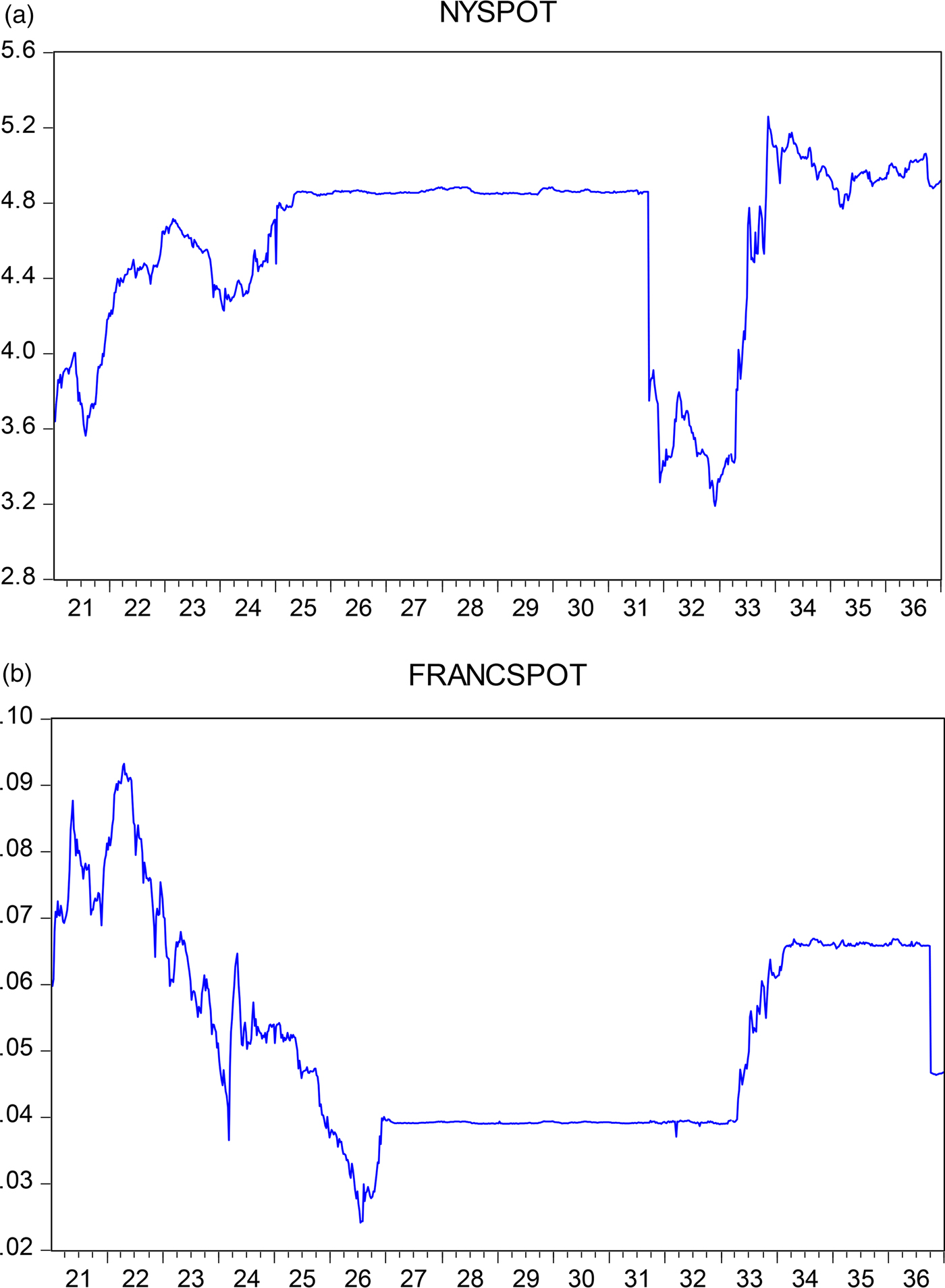
Figure 1. Pound–dollar exchange rate, spot 1921–36 (weekly data)
The rest of the article is organized as follows: in Section ii I discuss the path to dollar devaluation in 1933, a process that began on 6 March, when President Roosevelt declared a national banking holiday. The section includes a detailed analysis of the ‘gold-buying’ program questioned by Keynes in his open letter. In Section iii I deal with the dollar–pound exchange rate. I display and analyze the basic data, and I use Markov switching regressions with regime-dependent variances to study whether the extent of volatility during the gold-buying program was higher than during other times within the 1921–36 period. In Section iv I turn to the dollar–franc and present the Markov switching regressions for this bilateral exchange rate. Section v contains closing remarks. Here I discuss the adoption of the Gold Reserve Act of 1934, and Keynes's reaction to the fixing of the price of gold at $35 an ounce. There are also two appendixes. In Appendix A, I put Keynes's advice in the open letter in perspective, by (briefly) analyzing his evolving policy views on exchange rates and gold. I point out that Keynes's plan for the international monetary system was similar to a plan developed by James P. Warburg, a close adviser of President Roosevelt. In Appendix B I present the data sources.
II
II.1 From the gold embargo to the London Monetary and Economic Conference
In the early hours of 6 March 1933, when he had been in office barely one day, President Roosevelt declared a national banking holiday, and implemented a gold embargo. The purpose of this policy was to stop massive withdrawals of currency and gold, and to put in place an emergency plan to strengthen the nation's financial system.Footnote 6 The Secretary of the Treasury, Will Woodin, justified the embargo by saying that ‘gold in private hoards serves no useful purpose under current circumstances. When added to the stock of the Federal Reserve Banks it serves as a basis for currency and credit. This further strengthening of the banking structure adds to its power of service toward recovery.’Footnote 7 On 9 March Congress passed the Emergency Banking Act, which gave authority to the government to liquidate insolvent banks and to provide support to those that were viable in the long run. On 13 March, banks began to reopen their doors, and the public started to re-deposit their cash and gold in massive amounts.Footnote 8 Although (most) banks opened gradually, the gold embargo remained in place. Three weeks later, on 5 April, President Roosevelt issued an Executive Order requiring people and businesses to sell, within three weeks, all their gold holdings to the government at the official price of $20.67 per ounce. Footnote 9
On 19 April, during the thirteenth press conference of his young presidency, President Roosevelt stated unequivocally that the country was now off the gold standard. Gold exports were prohibited. He declared that the fundamental goal of abandoning the monetary system that had prevailed since Independence was to help the agricultural sector, which had been struggling for over a decade. He stated: ‘The whole problem before us is to raise commodity prices.’Footnote 10
The next step in the path towards devaluation came on 12 May, when Congress passed the Agricultural Adjustment Act (AAA). Title iii of this legislation included the ‘Thomas Amendment’, which authorized the President to increase the official price of gold to up to $41.34 an ounce.Footnote 11 A devaluation of the dollar, many thought, would rapidly result in ‘controlled inflation’ and would help farmers by raising commodity prices and by lightening their debts when expressed in relation to their incomes. A number of analysts noted that Great Britain had devalued the pound in September 1931, and had slowly begun to recover. They also pointed out that after devaluing sterling the UK had established a currency stabilization fund – the Exchange Equalization Fund.
However, there was a major difficulty in devaluing the dollar officially: most debt contracts – both private and public – included a ‘gold clause’, stating that the debtor committed himself to paying back in ‘gold coin’. If the currency was devalued with respect to gold, the dollar value of debts subject to the gold clauses would automatically increase by the amount of the devaluation. This would result in massive bankruptcies and in a huge increase in the public debt. On 5 June, Congress passed Joint Resolution No. 10, annulling all gold clauses from future and past contracts. This opened the door for a possible official devaluation.Footnote 12
One week after debt contracts were changed by Congress, on 12 June, the London Monetary and Economic Conference was inaugurated by the King. The conference was supposed to last for twelve weeks and to deal with an array of issues, including international trade, credit policies, employment, protectionism, commodity prices, and the possible return of all nations to an ‘international standard’.Footnote 13 A key question addressed by representatives of the three largest economies – the US, Great Britain and France – was whether exchange rates should be stabilized during the duration of the conference. France's position was that without stabilization it was impossible to make progress on the other issues. The US and the UK were not opposed, in principle, to (temporary) stabilization. The question was at what rates to do it. This issue was negotiated in tripartite meetings that operated parallel to the official conference.Footnote 14
On 3 July, the conference delegates were shocked by a message sent by President Roosevelt. He wrote that he was dismayed by the direction the discussions had taken. There was too much emphasis on short-run exchange rate stabilization and not enough on commodity prices and recovery. He added that the US would not participate in any effort to stabilize the exchanges in the immediate run, and that the conference's fixation with short-term stability responded to ‘old fetishes of so-called international bankers’.Footnote 15 He declared that the aim of the parley ought to be generating mechanisms for ‘controlled inflation’.Footnote 16 Following Roosevelt's message – known as the ‘bombshell’ – the conference stalled, and three weeks later it adjourned without achieving any of its goals, not even the most modest ones.
The London Monetary and Economic Conference of 1933 marks a major turning point in President Franklin D. Roosevelt's policies towards gold and exchange rates; there is a ‘before London’ and an ‘after London’. After the conference, US policy towards the dollar became proactive and experimental; between October 1933 and January 1934 it was based on a program aimed at manipulating the world price of gold.
II.2 The gold-buying program of October 1933
As noted, during his first year in office, President Roosevelt repeatedly stated that one of the most important goals of his administration was to raise commodity prices. For example, on 19 April 1933, after announcing that the US was abandoning the gold standard, he said:Footnote 17
The whole problem before us is to raise commodity prices. For the last year, the dollar has been shooting up [this was a reference to the depreciating pound sterling] and we decided to quit competition. The general effect probably will be an increase in commodity prices. It might well be called the next step in the general program.
During the first half of August 1933 the President met several times with George F. Warren, a professor of agricultural economics at Cornell University, to discuss commodity markets. In Reference Warren and Pearson1931 Warren and his colleague Frank I. Pearson had published a book, Prices, where they analyzed price behavior for a score of products and countries during more than one hundred years.Footnote 18 Their conclusion was that individual commodity prices went up and down because the world's stock of monetary gold increased and decreased through time. According to their results, the correlation between these variables was extremely high, almost perfect. This meant, they argued, that the easiest way to raise commodity prices was by increasing the dollar price of gold. Warren and Pearson emphasized that their approach had nothing to do with traditional monetary theory. For them, what the Federal Reserve did was rather irrelevant, as were the quantity theory of money and the equation of exchange.Footnote 19
In mid August, President Roosevelt decided to put Warren's theories to work, and asked Dean Acheson, the acting Secretary of the Treasury, to ‘try his hand at a draft (for discussion only) of an Executive Order offering to buy newly minted gold for 30 days at a fixed price say $28 an ounce and an offer to sell gold to the artists and dentists at the same price’.Footnote 20 At the time the official price of gold was $20.67. Two weeks later, on 29 August, Executive Order No. 6261 was issued. The Secretary of the Treasury would now accept newly minted gold for sale on consignment. This metal could be sold to individuals authorized to acquire the metal – artists and dentists. The purchase price would be ‘equal to the best price obtainable in the free market of the world after taking into consideration any incidental expenses such as shipping costs and insurance’.Footnote 21 The expectation was that by buying gold at the ongoing world price – which was higher than the ‘official’ price of $20.87 an ounce – agricultural prices would increase rapidly. Throughout September, however, commodity markets continued to be depressed. By the end of the month the price of corn was 28 percent lower than on 15 July; the prices of cotton, rye and wheat had declined by 13, 30 and 21 percent relative to that date.
On Sunday 22 October, FDR delivered his Fourth Fireside Chat. He reiterated that the definitive goal of the government was to ‘restore commodity price levels’.Footnote 22 He said that in order to accomplish this goal he had decided to expand the gold-buying program. The Reconstruction Finance Corporation (RFC) would buy newly minted gold at prices determined from time to time by the Secretary of the Treasury and the President. If needed, the RFC would also buy and sell gold in the world market at these prices. The most important difference between this new gold-buying program and the one established on 29 August was that under the original plan gold purchases were at ongoing world prices, while the new initiative permitted the government to set any price it wanted, and to alter it as frequently as it desired.Footnote 23
On 25 October, the first day of the program, the RFC paid $31.36 per ounce of gold, 27 cents above the world price. During the next 45 days or so, FDR, with Professor George F. Warren's assistance, determined every morning the price at which the RFC would buy gold during that day; almost always at a premium over the world price.
The RFC made its first international purchase on 1 November, when it bought a small batch of gold in France at $32.36 an ounce.Footnote 24 On 9 November, Jesse Jones, the chairman of the RFC, informed the press that since the launching of the program the corporation had bought 213,000 ounces of newly minted gold domestically. He stated that the amount of gold bought in global markets was modest, but refused to divulge the exact amount. That day the price offered was $33.15 per ounce, 10 cents higher than the international market price. On 15 November, an informed source who did not want to be identified stated that to that date purchases abroad had amounted to only $6 million. By late December the RFC was paying $32.61 per ounce of gold.Footnote 25
In early January 1934, almost coincidentally with the publication of Keynes's open letter, the gold-buying program was effectively ended.Footnote 26 On 31 January 1934, one day after the Gold Reserve Act of 1934 was signed into law, the President set the new official price of gold at $35 an ounce. The Treasury would buy and sell internationally any amount of metal at that price, in order to settle trade payments. Americans, however, were still forbidden from holding gold. This price was in place until mid 1971. See Section v for a further discussion on the Gold Reserve Act.
III
Before proceeding to the empirical results, it is important to discuss which exchange rate Keynes had in mind when he penned his open letter. Was he alluding to the bilateral rate between the dollar and sterling? Was he thinking of the dollar–gold rate? Or was he focusing on a weighted average rate that included various currencies?Footnote 27 According to Skidelsky (Reference Skidelsky1992, p. 493), in the second half of 1933 Keynes was mostly concerned with the volatility of the dollar-pound rate. More specifically, he thought that a US short-term policy goal should be ‘to keep the dollar-sterling exchange rate as stable as was consistent with an accelerating programme of loan-financed public expenditure’.Footnote 28 Skidelsky's views are supported by Keynes's own writings. Earlier that year, on 4 July, he published an article in the Daily Mail where he discussed FDR's ‘bombshell’ communiqué to the London Conference. In this piece Keynes supported FDR's decision to oppose short-term stabilization of the dollar, relative to gold, at a level that was inconsistent with higher commodity prices. But he added an important caveat. The President, he wrote, ‘would be unwise…to reject every plan, however elastic it is, for regulating the dollar –sterling exchange’.Footnote 29
This emphasis on the stability of the bilateral dollar–pound exchange rate was a short-term consideration. For the longer run, Keynes believed that all nations should try to stabilize their currency values relative to gold. He presented a specific plan for a new international financial system in the pamphlet The Means to Prosperity, published in March of 1933. He referred to this plan as a ‘qualified return to the gold standard’. Under it, he asserted, ‘stability of the foreign exchanges… would ensue’.Footnote 30 In Appendix A of this article I discuss Keynes's proposal, and I compare it with a plan independently developed in mid 1933 by FDR's adviser James P. Warburg.
III.1 Preliminary analysis for the dollar–pound
In the rest of this section I analyze the extent of volatility of the dollar–pound exchange rate during 1921–36. As noted, the main purpose of this analysis is to assess whether, as Keynes argued in his open letter, during the gold-buying program of 1933 the dollar became excessively volatile. In Section iv, I expand the analysis to the dollar–franc bilateral exchange rate.
Figure 2 presents the weekly percentage change of the pound–dollar exchange rate. Visual inspection suggests four chronological phases.Footnote 31 (1) A volatile period before the return of the UK to gold. This phase goes from January 1921 to April 1925. (2) A (very) tranquil period corresponding to the time when both the US and the UK were on the gold standard, from May 1925 to September 1931. During this phase exchange rate changes were minimal and stayed within the ‘gold points’. (3) A turbulent period following the abandonment of gold by the UK in September 1931. This volatile period continued after the abandonment of gold by the US in April 1933, and lasted until late January 1934. Notice that the ‘gold-buying’ program takes place towards the end of this phase, and is highlighted by a shaded area in Figure 3 (25 October – 31 December 1933). And (4), a period of limited variability which took place after the Gold Act was passed by the US Congress on 30 January 1934.
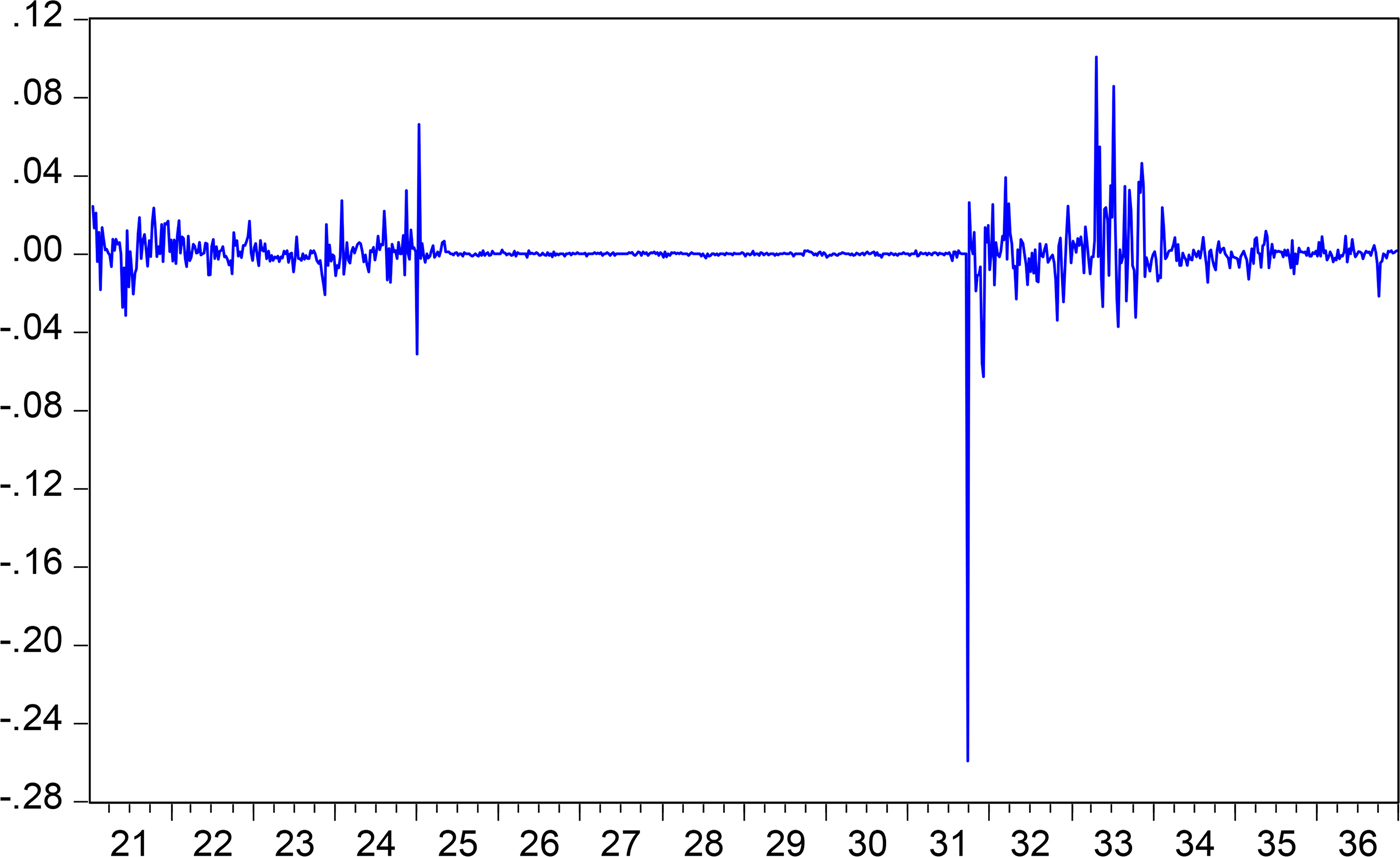
Figure 2. Weekly percentage change pound–dollar rate

Figure 3. Regime-smoothed probabilities, dollar–pound: weekly data, 1921–36
As a preliminary step, in Table 1 I present descriptive statistics for five subperiods, and for the complete period, 1921–36. In addition to the four chronological phases mentioned above, I have included the period that extends from the announcement that the US was off gold (19 April 1933) to the effective end of the London Conference, with FDR's ‘bombshell’ (4 July 1933). As may be seen, there are significant differences across subperiods. For instance, the standard deviation corresponding to the gold-buying period is among the highest of all subperiods. In Table 2 I report on a battery of tests for the equality of variances between the gold-buying program (25 October – 31 December 1933) and 1921–5 and 1931–3. The results in Panel A indicate that the null hypothesis of equality of variances is rejected under all tests for the comparison of the gold-buying program and first turbulent period (1921–5). On the other hand, as may be seen in Panel B, the null of equality of variance during the gold-buying program and the post-UK gold period (September 1931 – October 1933) cannot be rejected in three of the four tests.Footnote 32
Table 1. Dollar–pound exchange rate, 1921–36 (weekly percentage changes a )

a A positive number denotes a depreciation of the dollar; a negative number is an appreciation of the dollar and a depreciation of the pound.
Table 2. Test of equality of variances: dollar–pound A. Between the period 8 January 1921 – 25 May 1925 and gold-buying program (23 October – 31 December 1933)
B. Between the period 21 September 1931 – 20 October 1933 and gold-buying program (23 October – 31 December 1933)
III.2 Markov switching regressions: weekly data, 1921–36
In this subsection I present the results from the estimation of Markov switching regressions with regime-dependent variances to identify periods with different degrees of exchange rate volatility. As noted, I use weekly data for 1921–36. An advantage of this methodology is that the researcher does not incorporate his priors into the analysis; instead of arbitrary defining (and comparing) different volatility phases, the data are asked to determine how many distinct volatility regimes may be identified. The data are also asked at which dates the degree of volatility switched across regimes. The basic Markov-switching model with regime dependent variances has the following form:Footnote 33
 $$dlog{\rm} \, x_t = \gamma \left( k \right) + \sigma \left( k \right)\varepsilon _t$$
Where dlog x t is the weekly percentage change of the pound–dollar rate, γ(k) is a linear regression function that may depend on the k regimes, ε t is an iid normally distributed error term, with a standard deviation that is also regime dependent and may exhibit some form of autocorrelation. This type of switching volatility model was developed by Hamilton and Susmel (Reference Hamilton and Susmel1994), and has been used by Edwards and Susmel (Reference Edwards and Susmel2001), among others, to analyze exchange rate volatility around turbulent periods. In Markov models the regime probabilities p(k) are assumed to depend on the previous state (Hamilton Reference Hamilton1989):
 $$P\left( {s_t = i{\rm \vert} s_{t - 1} = j} \right) = p_{\,ji} \left( t \right) = p_{\,ji} \left( t \right). $$
The intercept in γ(k) in equation (1) is regime dependent and may be interpreted as (partially) capturing the degree of risk aversion in each regime. We anticipate that in the case at hand there will be, at least, two regimes: one corresponding to very low volatility, which would include the years when both countries were under the gold standard, and a different, high volatility state, when one of the two nations (or both of them) was off gold. The key question is whether it is possible to identify more than one turbulent regime. If this is the case, we are interested in understanding which of these volatile regimes the gold-buying program belongs to. More specifically, the question is whether the gold-buying period corresponds, as Keynes suggests in his letter, to the regime with the highest volatility or whether, on the contrary, it falls in the regime with intermediate volatility.
Base case results
In the base case estimates I allow for a regime-dependent intercept, a lagged dependent variable and regime-dependent variance. The error is assumed to have a common AR(1) term. Hansen likelihood tests indicate that the best characterization of the period under study corresponds to three regimes.Footnote 34 The results for the Markov regressions are given in Table 3: Regime 1 corresponds to intermediate volatility; Regime 2 to low volatility; and Regime 3 to high volatility. All estimates of the regime-dependent variance, log (sigma), are significant at conventional levels, as are the coefficients for the lagged dependent variables, and the common AR(1) term. When slightly different specifications were used, three regimes were still identified and the relative values of the coefficients were maintained (more on this below). As may be seen in Table 3, the differences in the extent of volatility across the three regimes are significant: the estimated variance during the high-volatility regime is 7.3 times higher than the estimated variance for the intermediate volatility regime. The latter is, in turn, 8.4 times higher than the estimated variance during the tranquil period.
Table 3. Markov switching regression, dollar–pound: 1921–36, regime-dependent variances
Table 4 provides a summary of the transitional probabilities and the regimes’ duration. As may be seen, the diagonal probabilities are very high, indicating that there is significant regime persistence. This table also shows that there is a 17.5 percent probability that if the system is in the high-volatility regime, the following week it will be in the intermediate-volatility one. The probabilities of moving from some degree of volatility (either intermediate or high) to tranquility, or vice versa, are very low. As anticipated, the low-volatility regime has the longest expected duration, at 139 weeks. The expected duration of high-volatility regimes is 18.2 weeks, and that of intermediate volatility is only 5.7 weeks.
Table 4. Markov transition summary, dollar–pound: transition probabilities and regime duration

Figure 3 contains the smoothed regime probabilities corresponding to the base-case estimates. As expected, the low-volatility regime (Regime 2) is correctly identified as the period when both nations were on the gold standard and the dollar–pound exchange rate moved within the gold points. As expected, the post-Gold Reserve Act of 1934 period – when a new official price of gold in the US was set at $35 an ounce – corresponds to intermediate volatility; during this period the pound was still off gold and fluctuated according to market forces (although the British intervened from time to time through their Exchange Equalization Fund, established on 19 April 1932). As may be seen, between September 1931 and January 1934, there are several shifts from high to intermediate, and back to high volatility. In addition, and as is shown in greater detail below, the system moves into high volatility at the beginning of the gold-buying period, but half way through it, it switches back to intermediate volatility.
In order to analyze in greater detail regime switches during the latter part of 1933, in Figure 4 I zoom in on the transitional probabilities for the intermediate and high-volatility regimes between 1 August and 31 December 1933. For expository reasons I have excluded the low-volatility probabilities; they are mostly zero during these 24 weeks. This figure shows that the system moved into the high-volatility regime during the last week of August, at the time the original gold-buying program, which purchased metal at ongoing world prices, was announced and launched (Executive Order no. 6261). The dollar–pound rate stayed on the high-volatility regime until the last week of November, when it switched to intermediate volatility. That is, Keynes was right in pointing out that the gold-buying program generated high-dollar ‘gyrations’, but what he failed to notice (or to mention) is that towards the end of the period this volatility had abated, and that the pound–dollar rate was back to an intermediate volatility regime. Keynes also failed to mention that although during the gold-buying program the dollar–sterling bilateral rate was characterized by high volatility, this was not higher than during other periods around that time. As may be seen in Figure 4, the dollar–sterling rate was also in a high-volatility regime for several weeks after the UK abandoned gold in September 1931, and for some weeks during 1921 and 1924–5.Footnote 35 According to this analysis, it is not possible to identify a different regime (with even higher volatility) during the gold-buying program.

Figure 4. Regime-smoothed probabilities, dollar–pound: weekly data, August–December 1933
An interesting question is why volatility declined towards the end of November 1933. The most plausible explanation is that the administration realized that the discretionary way in which the RFC prices were determined generated heightened uncertainty. It was around that time when Jacob Viner – the respected University of Chicago professor, who would become an adviser to the Treasury in 1934 – wrote a longish memorandum to Henry Morgenthau, Jr (then the acting Secretary of the Treasury), where he explained that the gold-buying program was not working as promised. A serious problem, Viner asserted, was that the purchases abroad were too small, and did not really change the international price of gold. In addition, the discretionary changes in the price of gold, and the absence of a clear program geared towards stabilization, were encouraging speculation, and negatively affecting investment decisions.Footnote 36 Starting in mid December, daily prices paid by the RFC changed more gradually, and the RFC premium became smaller and more stable. Data from the forward markets for the dollar relative to several currencies, collected by Einzig (Reference Einzig1937), suggest that starting in the second week of December the market began to sense that a major change to the exchange rate regime was in the works.Footnote 37
Robustness and extensions
In order to test for the robustness of the results reported above, I estimated a number of Markov-switching regressions with alternative specifications. In particular, I introduced additional regressors, including the one-month forward premium in the exchange rate market (see Appendix A for data sources). As may be seen from Table 5, the coefficient for this variable is significantly positive. More importantly, the results regarding the number of regimes, the relative sizes of the variance in each of them and the transitional probabilities are very similar to those reported in the base case estimates and discussed above, and provide support for the main conclusions of the analysis. Notice that in Table 5 the forward premium was introduced as a regressor that is not regime dependent. However, if it is included as depending on the regime, the results are very similar, and don't affect the conclusions in any significant way (results available on request).
Table 5. Markov switching regression, dollar–pound: 1921–36, regime-dependent variances, alternative specification
I also analyzed whether there were switches in the volatility regime around important dates during 1933–4. In addition to the gold-buying program I considered: (a) the passage of the Emergency Banking Act on 9 March 1933; (b) the President's announcement that the country was off gold on 19 April; (c) the approval of the Thomas Amendment on 12 May; (d) Congress's joint resolution of 5 June, abrogating the gold clauses; (e) the inauguration of the London Monetary and Economic Conference on 12 June; and (f), the passage of the Gold Reserve Act of 1934. The results from the Markov switching regressions indicate that there were switches in the volatility regime around three of these events (see Figure 3): the abandonment of the gold standard (19 April), the gold-buying program (October and December 1933) and approval of the Gold Reserve Act of 1934.Footnote 38
I also invesigated whether some of the important political events during 1921–36 were reflected in switches of volatility regime. In particular, I focused on changes in government in the three main powers of the time – the US, the UK and France. No significant mapping from these events to volatility switches was found before 1933. I also inquired whether the ascendance of the Nazis in Germany was, in any way, reflected in volatility switches. The results suggest that shortly after Hitler became chancellor, the dollar–pound moved to high volatility. It is difficult, however, to fully ascribe that development to politics in Germany, since at almost exactly the same time the US was going through major financial upheaval, including the declaration of the national banking holiday in early March 1933.Footnote 39
IV
In this section I expand the analysis to the dollar–franc. In Figure 5 I present the weekly percentage change in this bilateral exchange rate. In Table 6, on the other hand, I present the Markov switching regression results. Figure 6 contains the smoothed transitional probabilities.Footnote 40
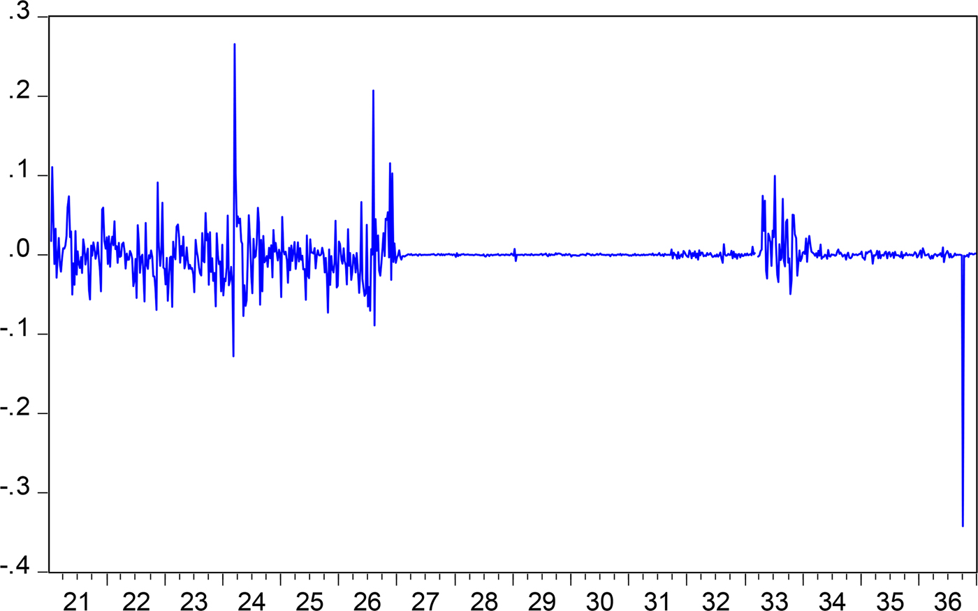
Figure 5. Weekly percentage change franc–dollar rate, 1921–36

Figure 6. Regime-smoothed probabilities, dollar–franc: weekly data, 1921–36
Table 6. Markov switching regression, dollar–franc: 1921–36, regime-dependent variances

In this case it is also possible to identify three volatility regimes. Regime 1 corresponds to low volatility, Regime 2 is for high volatility, and Regime 3 to intermediate volatility. As may be seen from Table 6, the coefficient for the log of the variances is always significant, as is the common AR(1) term. When alternative specifications are used – for instance, when the forward premium is included – the results are very similar to those reported in Table 6. Expected durations for the three regimes are as follows: Regime 1 (low volatility), 30.3 weeks; Regime 2 (high volatility), 55.9 weeks; and Regime 3 (intermediate volatility), 15.1 weeks; notice that these durations are quite different from those for the dollar–pound reported in Table 4. For the dollar–franc bilateral exchange rate the three regimes exhibit a significant degree of persistence; the diagonal elements in the transition matrix are very high: 0.967, 0.982 and 0.933.
The smoothed transitional probabilities, presented in Figure 6, are particularly interesting: as may be seen, and as expected, the dollar–franc rate exhibits low volatility during most of the December 1926 – September 1931 period. This phase begins with France's return to the gold standard, and ends when the UK came off gold. Between late September 1931 and mid April 1933 – when FDR took the US off gold – the dollar–franc rate is in the intermediate volatility regime. This is an interesting result, which suggests that once the UK abandoned the gold standard, the market became somewhat skittish about the dollar. Indeed, at the time some market participants believed that the US would follow the UK, and come off gold.Footnote 41
On the week of 22 April 1933 – immediately after FDR made the announcement that the US was officially off gold – there is significant jump in regime probabilities: the probability of being in the intermediate regime declined from 0.912 to almost zero, and the probability of being in the high-volatility regime jumped from 0.091 two weeks earlier to almost 1.0.
The results in Figure 6 indicate that when the first phase of the gold-buying program was launched in late August 1933, the dollar–franc rate was already in the high-volatility regime (the probability had been close to 1.0 since 22 April 1933). The results also show that in mid December – in the midst of the gold-buying program – there was a significant decline in the probability of being in the high-volatility regime. According to these estimates, during the week of 2 December, the probability of being in the high-volatility regime was almost equal to 1.0; a week later, on 9 December, that probability had declined to 0.48; and in the week of 16 December it had dropped further to 0.24. By the end of the year (30 December) the probability of the dollar–franc exchange being in the high-volatility regime was a low 0.15. During that same week the probability of being in the intermediate probability regime had climbed to 0.83, from almost zero four weeks earlier.
A comparison of Tables 3 and 6 shows that two bilateral exchange rates (dollar–pound and dollar–franc) exhibit some similarities, as well as some differences. The most important similarity is that in mid December 1933, both the dollar–pound and dollar–franc went through a switch in volatility regime, moving from high to intermediate. This happened while the gold-buying program was still in effect and before Keynes wrote his open letter. Two important differences are: the dates at which volatility switches occur are not the same in the two cases; also, the extent of volatility in the different regimes (as measured by the point estimate of log (sigma)) is somewhat different across the two exchange rates.
V
On 30 January 1934, and after a heated debate in both chambers of Congress, the Gold Reserve Act of 1934 was signed into law. The next day the President set the new official price of gold at $35 an ounce, and the Treasury announced that for the foreseeable future it was willing to buy and sell any amount of metal at that price, internationally. Residents of the United States, however, were not allowed to hold gold. This official price of $35 an ounce was in effect until August 1971, when President Richard Nixon closed the Treasury's ‘gold window’.
A key component of the Gold Reserve Act was the creation of an Exchange Stabilization Fund at the Treasury.Footnote 42 The fund was, to a large extent, tailored after the British Exchange Equalisation Fund, and its main objective was to intervene, under well-defined circumstances, in the global currency markets. The purpose of these interventions was to reduce excessive volatility – something that, as argued, was close to Keynes's heart – and to ensure that the exchange rate would stay within a very narrow window around $35 per ounce of gold. The Stabilization Fund was originally funded with $2 billion, corresponding to the Federal Reserve profits from the revaluation of the price of gold from $20.67 to $35 an ounce.Footnote 43
After the passage of the Gold Reserve Act, monetary conditions in the US changed drastically. Between January and December 1934 the stock of monetary gold more than doubled; it went from $3.9 billion to $8.1 billion. Part of this increase – a little over $2.5 billion – was the result of revaluing the stock of bullion at $35 an ounce. But more important than repricing were the large amounts of gold that came into the country immediately after the Gold Reserve Act was passed in late January 1934. More than $750 million flew in during February alone – $239 million from London, $124 million from Paris – another $262 million came in during March, and $155 million in April.Footnote 44
An important question is, how influential was Keynes's letter in the adoption of the Gold Reserve Act? Moggridge (Reference Moggridge1992 p. 581) argues that ‘the general conclusion seems to be that it [the letter] had little, if any effect’. This view is supported by a letter written by President Roosevelt to Felix Frankfurter on 22 December 1933. Here, the President makes a brief reference to ‘the professor's' [Keynes's] views on public works, but is completely silent regarding his exchange rate comments.Footnote 45 In a letter to Keynes, written on 17 April 1934, Walter Lippmann points out that the letter had influence on the Treasury's decision to purchase long-term government bonds as a way of ‘reducing the long-term rate of interest’. In this letter, however, Lippmann does not say a word on exchange rates or gold.Footnote 46
In light of his open letter, why didn't Keynes criticize the Gold Reserve Act, a piece of legislation that rigidly fixed the price of gold? In the New York Times piece he expressly wrote that FDR should reject the temptation to ‘devalue the dollar in terms of gold, returning to the gold standard at a new fixed ratio’. A possible answer is that in Keynes's eyes the Gold Reserve Act was not a return to the traditional gold standard. Indeed, under the Act gold was only used to settle international transactions, and could not be held, bought, or sold by American citizens, banks, or corporations. In that regard, the new regime was closer to Keynes's views of a modified gold standard. In an article published in the New Statesman and Nation on 20 January 1934, he argued that the official devaluation of the dollar would not harm the UK. However, he wrote, it could have serious implications for the gold bloc countries, whose currencies would now be seriously overvalued. It was possible, he noted, that France would be forced off gold. In spite of this, he provided a positive assessment of the overall situation created by the enactment of the Gold Reserve Act: ‘I cannot doubt but that the President's announcement means real progress. He has adopted a middle course between old-fashioned orthodoxy and the extreme inflationist. I see nothing in his policy which need be disturbing to business confidence’ (Keynes Reference Keynes and Moggridge1982, p. 312). Keynes further believed that as a consequence of the Gold Reserve Act, there would be a monetary conference attended by the US, Great Britain and France. Out of this gathering, he hoped, a new international system with stable, but not totally rigid, exchange rates would emerge. In his New Statesman and Nation article he wrote: ‘[T]he purpose of a monetary conference would not be to return to an old-fashioned gold standard… [T]he conference would presumably aim for the future not at rigid gold parities, but at provisional parities from which the parties to the conference would agree not to depart except for substantial reasons arising out of the balance of trade or the exigencies of domestic price policy.’Footnote 47
To summarize: the analysis presented in this article indicates that during the early weeks of the US gold-buying program of 1933, exchange rate volatility was very high, as pointed out by Keynes in his open letter. However, the results also unveil two features of this period not mentioned by Keynes. (1) During the gold-buying program volatility was not higher than during other turbulent subperiods in 1921–36. In that sense, exchange rates may have been ‘on the booze’ for longer than Keynes pointed out. (2) Towards the latter part of the gold-buying program, exchange rate instability declined significantly, with the system moving decisively from a high-volatility regime to an intermediate-volatility one.
This work may be extended in several directions. For instance, it is possible to use alternative techniques such as EGARCH models. Preliminary results, using that approach, tend to confirm those reported here, in the sense that in the middle of the gold-buying program there was a decline in volatility in both bilateral exchange rates. Another extension would be to move towards even higher-frequency data, focusing on daily exchange rate quotes. A possible shortcoming of that approach, however, is that at that frequency there is additional noise in the data. A third avenue for future research is to try to determine the role of exchange rate ‘fundamentals’ in currency behavior and volatility during these years. In this case, however, it would be necessary to move to monthly – or even quarterly – data, as data for most fundamentals are only available at those intervals.
APPENDIX A: DOLLAR VOLATILITY IN 1933, AND THE KEYNES AND WARBURG PLANS
When Keynes wrote his New York Times letter he already had a clear idea of the type of international monetary system that he wanted to see in place. He had discussed the problem in a number of his writings, including A Tract on Monetary Reform (Reference Keynes1923) and A Treatise on Money (Reference Keynes1930). But for the purpose of this article the most relevant exposition of Keynes's ideas is the one he presented in the 1933 pamphlet The Means to Prosperity, which reproduced in a revised and enlarged fashion four articles published in The Times of London during early 1933.Footnote 48 It is here where he lays down the bases of what would eventually become the ‘Keynes Plan’ discussed during the Bretton Woods Conference in 1944.Footnote 49
In 1923, in A Tract on Monetary Reform, Keynes wrote what became a famous quote: ‘In truth, the gold standard is already a barbarous relic… [I]n the modern world of paper currency and bank credit there is no escape from a “managed” currency, whether we wish it or not…’Footnote 50 However, Keynes's views evolved, and by late 1932 and early 1933 they were more nuanced.Footnote 51 In chapters iv and v of The Means to Prosperity he suggests that all major powers adopt a new standard and create an ‘international note issue’ linked to gold. These notes would be issued by a new ‘international authority’, and each country would obtain a quota of these notes in exchange for gold-denominated bonds issued by their governments.Footnote 52 Keynes wrote: Footnote 53
[T]he notes would be gold-notes and the participants would agree to accept them as the equivalent of gold. This implies that the national currencies of each participant would stand in some defined relationship to gold. It involves, that is to say, a qualified return to the gold standard.
According to Keynes's plan, central banks would have greater flexibility to undertake countercyclical policies, and the ‘gold points’ would be widened to 5 percent.Footnote 54 This wider range for the gold points was essential in order to avoid ‘wild movements of liquid funds from one international center to another’. The ‘international notes’ would greatly increase worldwide liquidity, and reduce central bankers’ apprehensions about ‘free gold’, or the amount of bullion over and above what was required to back the bank's monetary liabilities. Keynes also believed that a one-time depreciation of ‘national currencies’ with respect to gold – notice the plural, ‘currencies’ – would help increase ‘loan-expenditure’, as central banks would ‘be satisfied with a smaller reserve of international money’.Footnote 55 According to this plan, ‘stability of the foreign exchanges… would ensue’. The plan, however, allowed countries to alter their parity with respect to gold under extraordinary circumstances, such as major changes in ‘the international price level’. Keynes was clear to point out that these adjustments were extraordinary events; they ‘should not be allowed to occur for any other reason [except for major dislocations]’.
Keynes's plan was similar to a plan developed, somewhat independently, in 1933 by James P. Warburg, a banker and adviser to President Roosevelt. In preparation for the London Economic Conference – which, as noted, was inaugurated on 12 June 1933 – Warburg drafted a proposal for a new ‘international standard’ to be adopted by all nations. Gold would continue to be at the center of the global system, but the rules of the game would be different. There would be more flexibility and bullion itself would not be physically shipped from place to place. Silver would also have a role; up to 20 percent of central bank reserves could be maintained in the white metal. There would be no gold clauses, which tied debt contracts to the price of gold, and the ‘cover ratio’ would be reduced significantly in every country. The proposed new cover ratio was 25 percent, which in the US represented an important reduction relative to the existing 40 percent. This ‘modified gold standard’ would reestablish exchange rate order and would allow exporters, importers, bankers and investors to plan ahead their international businesses. Every country would declare a new parity and exchange rates would be pegged to each other. Competitive devaluation would be ruled out, and with the lower cover ratio central banks would have the ability to undertake expansive monetary policy during downturns, and thus avoid cycles of deflation.Footnote 56
APPENDIX B: DATA SOURCES
Spot exchange rates: Einzig Reference Einzig1937, appendix i.
Forward exchange rates: Einzig Reference Einzig1937, appendix i.
World price of gold: Warren and Pearson Reference Warren and Pearson1935, table 9, p. 169.
RFC price of gold: Warren and Pearson Reference Warren and Pearson1935, table 8, p. 168.


