


Introduction
Turfgrass managers rely on broadcast applications of selective postemergence herbicides to control emerged weeds, despite the nonuniform pattern of typical weed infestations (Jin et al. Reference Jin, Bagavathiannan, Maity, Chen and Yu2022a, Reference Jin, Bagavathiannan, McCullough, Chen and Yu2022b; Yu et al. Reference Yu, Schumann, Sharpe, Li and Boyd2020). Therefore broadcast applications result in a portion of the herbicide deposited to turfgrass canopy without the weed target (Monteiro and Santos Reference Monteiro and Santos2022). Site-specific weed management (SSWM) using manual spot applications directly to individual weeds minimizes herbicide losses but is labor intensive and often cost prohibitive (Heisel et al. Reference Heisel, Andreasen and Ersbøll1996; Rider et al. Reference Rider, Vogel, Dille, Dhuyvetter and Kastens2006). SSWM also often lacks sufficient accuracy and precision due to human error (Yu et al. Reference Yu, Schumann, Cao, Sharpe and Boyd2019a, Reference Yu, Sharpe, Schumann and Boyd2019b, Reference Yu, Sharpe, Schumann and Boyd2019c, Reference Yu, Schumann, Sharpe, Li and Boyd2020). Modern technologies have the capacity to achieve accurate and precise herbicide applications to spatially and temporally variable weed infestations (Monteiro and Santos Reference Monteiro and Santos2022). However, real-time recognition of the weed species and location of the weed (spatial distribution) remains a critical component.
Deep learning (DL) is a sophisticated, in-depth subset of machine learning through artificial intelligence. DL is based on the utility of artificial neural networks (ANNs), which are mathematical models patterned around the neural connectivity of a human brain (Greener et al. Reference Greener, Kandathil, Moffat and Jones2022; Janiesch et al. Reference Janiesch, Zschech and Heinrich2021). Convolutional neural networks (CNNs) are complex ANNs with the capacity to decipher grid-structured spatial relationships for automated learning of informative features with multiple levels of representation of such features (Greener et al. Reference Greener, Kandathil, Moffat and Jones2022; LeCun et al. Reference LeCun, Bengio and Hinton2015; Schmidhuber Reference Schmidhuber2015). Machine vision (MV) is the process of signal transfer from a sensing device (e.g., image capturing camera) into a digital form (Nasirahmadi et al. Reference Nasirahmadi, Edwards and Sturm2017). Paired with MV, CNNs have the potential for recognition of certain objects within an image (Greener et al. Reference Greener, Kandathil, Moffat and Jones2022; Janiesch et al. Reference Janiesch, Zschech and Heinrich2021; Zhang and Lu Reference Zhang and Lu2021) and can be used for automated differentiation between weeds and turf (Jin et al. Reference Jin, Bagavathiannan, McCullough, Chen and Yu2022b).
CNNs were first introduced for weed recognition in turf by Yu et al. (Reference Yu, Sharpe, Schumann and Boyd2019c). Researchers initially focused on the use of image classification networks like AlexNet, DenseNet, EfficientNetV2, GoogLeNet, MobileNet-v3, RegNet, ResNet, ShuffleNet-v2, and visual geometry group neural network (VGGNet), which provide information on the presence or absence of the target weed in the image but lack the ability to discriminate the area within the image occupied by the weed. These networks have been shown to successfully recognize various broadleaf and grassy weeds in bermudagrass, bahiagrass (Paspalum notatum Flueggé), and perennial ryegrass (Lolium perenne L.) turf (Jin et al. Reference Jin, Bagavathiannan, Maity, Chen and Yu2022a, Reference Jin, Bagavathiannan, McCullough, Chen and Yu2022b; Yu et al. Reference Yu, Schumann, Cao, Sharpe and Boyd2019a, Reference Yu, Sharpe, Schumann and Boyd2019b, Reference Yu, Sharpe, Schumann and Boyd2019c, Reference Yu, Schumann, Sharpe, Li and Boyd2020).
Object detection networks are more precise than image classification networks, with the ability for target recognition and location within the image (Medrano Reference Medrano2021; Xie et al. Reference Xie, Hu, Bagavathiannan and Song2021; Yu et al. Reference Yu, Schumann, Cao, Sharpe and Boyd2019a, Reference Yu, Sharpe, Schumann and Boyd2019b, Reference Yu, Sharpe, Schumann and Boyd2019c). These networks include DetectNet, You Only Look Once (YOLO), Single Shot MultiBox Detector (SSD), and Faster R-CNN. Even greater precision can be attained with semantic segmentation models like Mask R-CNN, which have the ability to identify the exact shape of the target (Xie et al. Reference Xie, Hu, Bagavathiannan and Song2021). Object detection models have been used to successfully differentiate and identify actively growing clumps of annual bluegrass (Poa annua L.), henbit (Lamium amplexicaule L.), purple deadnettle (Lamium purpureum L.), and white clover (Trifolium repens L.) in fully dormant (i.e., straw-colored) bermudagrass (Yu et al. Reference Yu, Sharpe, Schumann and Boyd2019b, Reference Yu, Sharpe, Schumann and Boyd2019c) or common dandelion (Taraxacum officinale F.H. Wigg.) in perennial ryegrass (Yu et al. Reference Yu, Schumann, Cao, Sharpe and Boyd2019a) and bermudagrass (Medrano Reference Medrano2021). Semantic segmentation (Mask R-CNN, modified Mask R-CNN) was made by Xie et al. (Reference Xie, Hu, Bagavathiannan and Song2021) to detect nutsedge (Cyperus L.) plants in bermudagrass turf.
While the achievements in MV/DL-based technology in turf continue to evolve, integration with image capturing/processing systems and independent real-time, solenoid-actuated nozzles is the goal to achieve advanced SSWM—targeted spraying (Sharpe et al. Reference Sharpe, Schumann and Boyd2020). This technology has already been adapted for many crops, including rice (Oryza sativa L.), common sunflower (Helianthus annuus L.), sugar beet (Beta vulgaris L.), and carrot (Daucus carota L. var. sativus Hoffm.) (Hasan et al. Reference Hasan, Sohel, Diepeveen, Laga and Jones2021; Ma et al. Reference Ma, Deng, Qi, Jiang, Li, Wang and Xing2019), with estimates of 50% herbicide-use reduction when utilizing targeted spraying compared to broadcast applications (Thorp and Tian Reference Thorp and Tian2004). This technology cannot be readily applied to turfgrass because of differences in management and growth characteristics compared to agronomic crops; therefore, new turfgrass-specific approaches must be developed (Esau et al. Reference Esau, Zaman, Groulx, Corscadden, Chang, Schumann and Havard2016).
In turfgrass, the factual accuracy and precision of a targeted spraying system are dependent not only on the performance of its CNN component but also on the capacity of the application device to target the weed and avoid the crop. In real-world scenarios, an application pattern created by an individual nozzle in motion will be a linear strip of varying width (bandwidth) depending on the nozzle height and orifice angle (Villette et al. Reference Villette, Maillot, Guillemin and Douzals2021). As bandwidth increases, more area is covered, so the ability to precisely target small areas is limited compared to narrower bandwidths. Therefore, multiple nozzles comprising multiple narrow bandwidths should increase the precision and accuracy of the sprayer, because each nozzle can be operated independently to cover a smaller area (Jin et al. Reference Jin, Bagavathiannan, McCullough, Chen and Yu2022b; Villette et al. Reference Villette, Maillot, Guillemin and Douzals2021). However, identifying the proper nozzle density for a turfgrass-specific precision sprayer is crucial to achieving the compromise between maximized precision and accuracy and minimum installation and maintenance costs.
There were two primary objectives within the scope of this research. The first objective was to develop an object detection YOLO CNN model to detect complex spotted spurge patches structurally blended within highly infested bermudagrass turf maintained as a golf course fairway/athletic field. The second objective was to evaluate the impact of various nozzle densities on the YOLO CNN model efficacy and projected herbicide savings under simulated conditions. Spotted spurge was utilized as a target species for several reasons. It is found across a wide geographic area, making it applicable to many situations. Spotted spurge is an annual species with a high infestation capacity due to prolific seed production, late germination (often resulting in erratic control with preemergence applications), ability to survive under extremely close mowing conditions, and high recuperation capacity (Asgarpour et al. Reference Asgarpour, Ghorbani, Khajeh-Hosseini, Mohammadvand and Chauhan2015; McCullough et al. Reference McCullough, McElroy, Yu, Zhang, Miller, Chen, Johnston and Czarnota2016). This species serves as a good example of a low-growing broadleaf weed with small foliage that easily intertwines with turf canopy; thus it can pose difficulties for accurate weed detection using MV-based models. Spotted spurge allowed for the assessment of the YOLO algorithm’s potential to detect intricate weed structures entangled in turfgrass canopy as opposed to previously researched scenarios in which distinct weed patches were detected on contrasting backgrounds.
Materials and Methods
Image Acquisition
To ensure a diverse data set, images of various levels of spotted spurge infestation in ‘Latitude 36’ bermudagrass were collected from March to July 2021 at various times of day and week (i.e., at varying light conditions and randomly between mowing events) from two locations: the University of Florida (UF)/Institute of Food and Agricultural Sciences (IFAS) Fort Lauderdale Research and Education Center in Davie, FL (26.085°N, 80.238°W), and the UF/IFAS Plant Science Research and Education Unit in Citra, FL (29.409°N, 82.167°W). Turf at both locations was managed as a golf course fairway/athletic field. Standard maintenance was performed at each location and included mowing 3 d wk–1 at 1.3 cm with a reel mower with fertilization and irrigation according to UF Extension guidelines for each area.
Images were captured using a cell phone camera (iPhone 8 Plus, Apple Inc., Cupertino, CA, USA) via recording videos in MOV file format using 16:9 ratio. To ensure consistency in capturing uniform surface area, the camera was installed facing downward at a fixed height of 43.5 cm. The ground area represented in the recordings was 50.00 × 28.13 cm. Still frame images were then acquired from recordings via video extraction conducted using the FFmpeg (Free Software Foundation, Boston, MA, USA) script on a desktop computer (Dell OptiPlex 740, Dell, Round Rock, TX, USA) running an Ubuntu 18.04 operating system (Canonical USA, Dover, DE, USA). The script extracted still images from the videos at 4 frames s−1 with a pixel resolution of 1,280 × 720. Acquired still images were then subjectively selected to ensure balanced representation of captured weed encroachment levels, light conditions, and turfgrass canopy quality. As a result, a total of 1,291 still frame images for further model development/training (710 images for manual labeling and 481 images for automated labeling, totaling 1,191 images) and efficiency tests (the remaining 100 images) were acquired using the method described. To ensure diverse data sets, images for each step were selected randomly. During the entire process, unaltered individual images were not subject to more than one step, except when manually labeled images were pooled with autolabeled images for final CNN model training, as described later.
Model Development
A randomly selected subset of 710 of the extracted still frame images was labeled using bounding box drawing software compiled with Lazarus 1.8.0 (https://www.lazarus-ide.org/) to identify spotted spurge in turfgrass. Labeling consisted of a rectangle (“bounding box”) drawn around the outer margins of individual spotted spurge plants or their parts on the background of turfgrass canopy in each of the 710 images (Figure 1). The labeled subset of images was then used to train a YOLOv3 model to convergence (mAP = 87%) on the Darknet framework (Bochkovskiy et al. Reference Bochkovskiy, Wang and Liao2020). The YOLOv3-tiny-3l model was selected because of its compact size and high speed for real-time inferencing of video. The trained model was subsequently used to identify and autolabel spurge in a randomly selected 481 unlabeled images. A final model was trained with a combined data set of 1,191 labeled images consisting of 710 manually labeled images and 481 autolabeled images. The following Darknet hyperparameters (i.e., configuration variables to manage model training) were tuned prior to the model development to ensure the most optimal performance of the algorithm during the aforementioned training steps: 6,000 training iterations, batch size of 64 training images, subdivision of 16 training images, an exponential decay learning rate policy with 3,000 and 5,000 steps, and a base learning rate of 0.001.

Figure 1. Original still frame image with spotted spurge infestation in bermudagrass turf (A) and the same image manually labeled using bounding boxes drawn around the outer margins of individual target plants or their parts used for YOLOv3 model training (B).
Model Accuracy Assessment
Intersection over union was used to describe the ratio of overlap between the actual and predicted bounding boxes to establish if the detected object was a true positive (TP). Results were organized in a binary classification confusion matrix under four conditions: a TP, a false positive (FP), a true negative (TN), and a false negative (FN). Upon the completion of CNN training, the following parameters were computed using the aforementioned results to assess the new model’s accuracy in detecting spurge plants: precision (Equation 1), recall (Equation 2), and F1 score (Equation 3).
Precision (also called positive predictive value) is the number of correct results divided by the number of all returned results and describes how efficacious the new model is in positive (i.e., accurate) object (i.e., spurge) detection. Precision was calculated using the following equation (Hoiem et al. Reference Hoiem, Chodpathumwan and Dai2012; Sokolova and Lapalme Reference Sokolova and Lapalme2009; Tao et al. Reference Tao, Barker and Sarathy2016; Yu et al. Reference Yu, Schumann, Cao, Sharpe and Boyd2019a, Reference Yu, Sharpe, Schumann and Boyd2019b, Reference Yu, Sharpe, Schumann and Boyd2019c):
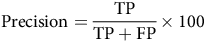 $${\rm{Precision}} = {{{\rm{TP}}} \over {{\rm{TP}} + {\rm{FP}}}} \times 100$$
Recall (also called sensitivity) is the number of correct results divided by the number of all results that should have been returned and describes how successful the new model is in correct target weed (i.e., spurge) identification. Recall was calculated by the following equation (Hoiem et al. Reference Hoiem, Chodpathumwan and Dai2012; Sokolova and Lapalme Reference Sokolova and Lapalme2009; Tao et al. Reference Tao, Barker and Sarathy2016; Yu et al. Reference Yu, Schumann, Cao, Sharpe and Boyd2019a, Reference Yu, Sharpe, Schumann and Boyd2019b, Reference Yu, Sharpe, Schumann and Boyd2019c):
 $${\rm{Recall}} = {{{\rm{TP}}} \over {{\rm{TP}} + {\rm{FN}}}} \times 100$$
The F1 score stands for the harmonic mean of the precision and recall values. The F1 score was determined using the following equation (Jin et al. Reference Jin, Bagavathiannan, Maity, Chen and Yu2022a, Reference Jin, Bagavathiannan, McCullough, Chen and Yu2022b; Sokolova and Lapalme Reference Sokolova and Lapalme2009; Yu et al. Reference Yu, Schumann, Cao, Sharpe and Boyd2019a, Reference Yu, Sharpe, Schumann and Boyd2019b, Reference Yu, Sharpe, Schumann and Boyd2019c):
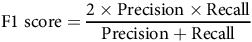 $${\rm{F1}}\;{\rm{score}} = {{2 \times {\rm{Precision}} \times {\rm{Recall}}} \over {{\rm{Precision}} + {\rm{Recall}}}}$$
Model Efficiency Assessment under Simulated Varying Nozzle Densities
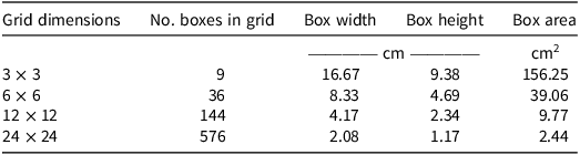
One hundred remaining unlabeled images were predicted with the trained YOLO model, and 50 output images (i.e., images labeled by newly trained YOLO model) were randomly selected for analysis. Each image was evaluated using a series of grids with a 3 × 3, 6 × 6, 12 × 12, and 24 × 24 matrix to simulate 3, 6, 12, or 24 nozzles, respectively, equally distributed on the spraying boom to cover the bandwidth of 50 cm total (Figure 2). This simulation was conducted under the assumptions that each individual nozzle remains open for the same time interval, the pattern and distribution is even and equal for each nozzle, and spray patterns do not overlap; thus the ratio of the sprayed area remains the same. Grids were created on separate layers in Adobe Photoshop (Adobe Systems, New York, NY, USA) and individually placed over each of the YOLO algorithm labeled images. This step created four new files per image and resulted in a total of 200 gridded labeled files for evaluation. The dimensions of each individual box within each grid matrix scenario were calculated based on actual total surface area captured in the photos (Table 1). The following data were manually collected for each grid-labeled file: (1) the number of grid boxes containing spurge regardless of detection (i.e., regardless, if labeled with bounding boxes; true infestation), (2) the number of grid boxes containing bounding box–labeled (i.e., detected) spurge only (true hits), (3) the number of grid boxes containing bounding box labels devoid of spurge (false hits), and (4) the number of grid boxes with spurge that was not labeled with bounding boxes (misses). This information was used to calculate the following variables for each grid:
 $$\small{{\rm{True}}\;{\rm{infestation}}\;{\rm{ratio}} = {{{\rm{Boxes}}\;{\rm{containing}}\;{\rm{spurge}}\;\left( {{\rm{true}}\;{\rm{infestation}}} \right)} \over {{\rm{Total}}\;{\rm{boxes}}\;{\rm{in}}\;{\rm{the}}\;{\rm{grid}}}} \times 100}$$
 $$\small {{\rm{True}}\;{\rm{hits}}\;{\rm{ratio}} = {{{\rm{Boxes}}\;{\rm{containing}}\;{\rm{spurge}}\;{\rm{with}}\;{\rm{labels}}\;{\rm{only}}\;\left( {{\rm{true}}\;{\rm{hits}}} \right)} \over {{\rm{Total}}\;{\rm{boxes}}\;{\rm{in}}\;{\rm{the}}\;{\rm{grid}}}} \times 100}$$
 $$\small{ {\rm{Misses}}\;{\rm{ratio}} = {{{\rm{Boxes}}\;{\rm{containing}}\;{\rm{spurge}}\;{\rm{with}}\;{\rm{no}}\;{\rm{labels}}\;{\rm{only}}\;\left( {{\rm{misses}}} \right)} \over {{\rm{Boxes}}\;{\rm{containing}}\;{\rm{spurge}}\;\left( {{\rm{true}}\;{\rm{infestation}}} \right)}} \times 100}$$
 $$\small{ {\rm{False}}\;{\rm{hits}}\;{\rm{ratio}} = {{{\rm{Boxes}}\;{\rm{with}}\;{\rm{labels}}\;{\rm{devoid}}\;{\rm{of}}\;{\rm{spurge}}\;\left( {{\rm{false}}\;{\rm{hits}}} \right)} \over {{\rm{Total}}\;{\rm{boxes}}\;{\rm{in}}\;{\rm{the}}\;{\rm{grid}}}} \times 100}$$

Figure 2. Original input image (left) and the same image with YOLOv3-generated bounding box spotted spurge predictions (right) with 3 × 3 (A, B), 6 × 6 (C, D), 12 × 12 (E, F), and 24 × 24 (G, H) grid matrixes demonstrating, respectively, 3, 6, 12, and 24 nozzles equally distributed on the spraying boom.
Table 1. Calculated grid dimensions for each photograph of spotted spurge in ‘Latitude 36’ bermudagrass turf
Data Analysis
Each photo (n = 50) was considered a separate experimental unit, grids were considered fixed variables, and images were considered random variables. Analysis of variance was performed using the PROC MIXED procedure in SAS version 9.4 (SAS Institute, Cary, NC, USA), and means for each fixed variable were compared using Tukey means comparisons at α = 0.05. Nonlinear regression was conducted in Sigma Plot (Systat Software, San Jose, CA, USA), and an exponential decay model was used to predict the relationship between the dependent variables and the number of boxes in the grid for each grid pattern:
 $$y = {y_0} + a{e^{ - bx}}$$
where y is the dependent variable, y 0 is the starting point, a is the scaling factor, e is the natural log, and −b is the rate of decay at box x.
Results and Discussion
Spotted Spurge Detection
Most of the prior work on the utility of CNN protocols in turfgrass has focused primarily on image classification algorithms like AlexNet, DenseNet, EfficientNetV2, GoogLeNet, ResNet, RegNet, ShuffleNet-v2, and VGGNet for the purposes of various broadleaf and/or grassy weed detection in bahiagrass, bermudagrass, and/or perennial ryegrass turf (Jin et al. Reference Jin, Bagavathiannan, Maity, Chen and Yu2022a, Reference Jin, Bagavathiannan, McCullough, Chen and Yu2022b; Yu et al. Reference Yu, Sharpe, Schumann and Boyd2019b, Reference Yu, Sharpe, Schumann and Boyd2019c, Reference Yu, Schumann, Sharpe, Li and Boyd2020). With the exception of GoogLeNet, which resulted in inconsistent weed detection (i.e., a variable F1 score ranging from 0.55 to 0.99), as reported by Yu et al. (Reference Yu, Sharpe, Schumann and Boyd2019c), the majority of image classification networks evaluated in those studies achieved an F1 score > 0.95 (Jin et al. Reference Jin, Bagavathiannan, Maity, Chen and Yu2022a, Reference Jin, Bagavathiannan, McCullough, Chen and Yu2022b; Yu et al. Reference Yu, Sharpe, Schumann and Boyd2019b, Reference Yu, Sharpe, Schumann and Boyd2019c, Reference Yu, Schumann, Sharpe, Li and Boyd2020). Being a harmonic mean between precision and recall, F1 score is a widely used CNN performance measure, with the maximum value of 1.00 indicating the model’s perfect fit and the minimum value of 0.00 indicating complete failure of the model (Zhao and Li Reference Zhao and Li2020). In general, the performance of CNN models is considered sufficient (i.e., the detection is considered successful) when F1 score > 0.50, good when F1 score = 0.80 to 0.90, and very good when F1 score > 0.90, while CNN models that achieve F1 score < 0.50 are considered poor or unsuccessful (Allwright Reference Allwright2022).
Unlike the image classification networks, the feasibility of object detection has not been extensively studied for turfgrass. However, in all researched cases, object detection models outperformed (i.e., achieved higher F1 scores when compared) image classification algorithms (Yu et al. Reference Yu, Sharpe, Schumann and Boyd2019b, Reference Yu, Sharpe, Schumann and Boyd2019c). Moreover, object detection algorithms have the capacity to locate the target’s position within the image and in that regard are superior to image classification (Jin et al. Reference Jin, Bagavathiannan, Maity, Chen and Yu2022a, Reference Jin, Bagavathiannan, McCullough, Chen and Yu2022b; Yu et al. Reference Yu, Schumann, Cao, Sharpe and Boyd2019a, Reference Yu, Sharpe, Schumann and Boyd2019b, Reference Yu, Sharpe, Schumann and Boyd2019c, Reference Yu, Schumann, Sharpe, Li and Boyd2020). Therefore, the YOLO object detection CNN was chosen for this research. Also, to date, all work on object detection architectures for turfgrass had been limited to recognizing weeds on contrasting backgrounds (either by color or by shape) and included the evaluation of (1) the DetectNet model for the ability to recognize various broadleaf species in contrasting color dormant bermudagrass (Yu et al. Reference Yu, Sharpe, Schumann and Boyd2019b, Reference Yu, Sharpe, Schumann and Boyd2019c) and (2) different versions of YOLO (YOLOv3; YOLOv4, and YOLOv5), SSD, and Faster R-CNN models for the detection of contrast in foliage shape of individual common dandelion plants (Medrano Reference Medrano2021). In this research, the focus was on the more complex scenario in which the target weed was structurally blended within the turfgrass canopy as opposed to forming distinguishable clumps on contrasting (either by color or by shape) backgrounds. However, the overarching purpose for developing an object detection–based model in this research was to achieve its sufficient performance, allowing for evaluating the model’s potential to cooperate with various nozzle density settings. Therefore, for this objective to be met, a minimum score of 0.50 in all the evaluated metrics was required. The object detection–based YOLO model used in this study achieved spotted spurge detection denoted by an F1 score of 0.62 (i.e., >0.50) resulting from precision of 0.65 and recall of 0.60 (Table 2). Therefore the minimum requirement is considered fulfilled, and this study is the first report of the successful recognition of diversified and complex weed patches formed by spotted spurge and intertwined in actively growing bermudagrass turf maintained as a golf course fairway or athletic field using an object detection algorithm. However, improvements in this model’s performance to allow it an achievement of fitness close to perfect (i.e., F1 Score of 1.00) are recommended and will be the subject of further research.
Table 2. Spotted spurge detection in ‘Latitude 36’ bermudagrass training results using the You Only Look Once (YOLO) real-time multiobject detection algorithm. a,b
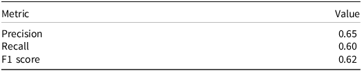
a Images for model development acquired from the UF/IFAS Plant Science Research and Education Unit in Citra, FL, and from the UF/IFAS Fort Lauderdale Research and Education Center in Davie, FL.
b Precision, recall, and F1 score values were obtained at the conclusion of 6,000 iterations for the experimental configuration.
In addition to general CNN performance, the target weed annotation process is an important aspect impacting CNN model development and training. Image classification procedures generally require high-volume imagery data sets. For example, Yu et al. (Reference Yu, Sharpe, Schumann and Boyd2019b) used 36,000 images for multispecies model training and up to 16,000 images for single-species training. In this study, the YOLO model was trained using only 1,191 training images and—as already discussed—resulted in successful detection of spotted spurge as denoted by an F1 score of 0.62 (i.e., >0.50) (Table 2). However, this method required creating bounding boxes that surrounded the entire individual target weed, resulting in time- and labor-intensive preparation of data sets. Other researchers (Yu et al. Reference Yu, Sharpe, Schumann and Boyd2019b) have noted the challenges of this approach, especially when individual plants are aggregated in larger patches. To overcome these issues, Xie et al. (Reference Xie, Hu, Bagavathiannan and Song2021) developed a bounding box/skeletal annotation method for nutsedge that takes advantage of the plant’s unique morphological characteristics. This model was not tested for other species or other weed groups that form dense mats in turf, suggesting that this technique may lack universality.
Sharpe et al. (Reference Sharpe, Schumann and Boyd2020) demonstrated that a simple change in annotation method from labeling the entire plant with a single bounding box to labeling small parts of the plant (partial annotation) using multiple bounding boxes drastically increased performance of goosegrass [Eleusine indica (L.) Gaertn.] detection in strawberry [Fragaria ×ananassa (Weston) Duchesne ex Rozier (pro sp.) [chiloensis × virginiana]] and tomato (Solanum lycopersicum L.). A similar approach was chosen for this study, resulting in the YOLO model’s capability of accurately recognizing spotted spurge patches of various shapes, sizes, and densities, as well as different levels of blending within turf canopy. The annotation may be further facilitated by using synthetic data sets and other data augmentation–based approaches in the future (Tong et al. Reference Tong, Wu and Zhou2020). However, this may be easier to achieve using semantic segmentation, where data are annotated precisely at the pixel level, allowing for outlining the actual boundaries between objects of similar spectral characteristics (Thorp and Tian Reference Thorp and Tian2004). Therefore, given the rapid advancement of information technology and engineering allowing for processing increasingly higher amounts of data in shorter time, various data set assembly strategies (particularly considering various ranges of image resolutions and/or dimensions) and annotation approaches will be considered in future investigations. The emphasis will be on more sophisticated annotation techniques, such as semantic segmentation, especially when coupled with the utility of synthetic data.
Effects of Grid Density on Spotted Spurge Detection
An efficient MV-based weed detection system is the foundation for the success of a targeted sprayer. However, to maximize the benefits of using such technology, a sprayer also needs to be capable of delivering herbicide to the detected target as accurately and precisely as possible (Jin et al. Reference Jin, Bagavathiannan, McCullough, Chen and Yu2022b). Although object detection algorithms enable precise localization of target weeds (Medrano Reference Medrano2021; Yu et al. Reference Yu, Sharpe, Schumann and Boyd2019b, Reference Yu, Sharpe, Schumann and Boyd2019c), the accuracy and precision of herbicide deposition on target plants are highly dependent on actuator characteristics (Villette et al. Reference Villette, Maillot, Guillemin and Douzals2021). The vast majority of herbicides currently used in turfgrass scenarios are systemic herbicides; thus it can be assumed that when a portion of a weed is sprayed, the herbicide will be translocated within the target plant and achieve kill, provided that the herbicide used has sufficient efficacy (Patton and Elmore Reference Patton and Elmore2021). Unless to compensate for imperfections of a spray system, as long as the sprayed area is not smaller than what the model has identified, there is no benefit to broadening the bandwidth. Therefore, when the sprayed bandwidth is wider than the weed plant/weed patch, assumption can be made that a portion of herbicide solution will be deposited off-target and wasted (Jin et al. Reference Jin, Bagavathiannan, McCullough, Chen and Yu2022b). In turfgrass, this “wasted” portion of spraying solution will be applied to the turfgrass canopy, which may lead to undesired outcomes. For instance, some of the chemistries currently allowed in turfgrass scenarios (e.g., to control challenging weed species) pose some risk of phytotoxicity even when applied accordingly with the label recommendations. One such example is topramezone-caused bleaching of bermudagrass canopy when applied to control goosegrass (Brewer and Askew Reference Brewer and Askew2021). Also, the development of such targeted spraying technology for turfgrass may allow for future use of nonselective herbicides with such systems, which will damage desired turfgrass outside of the target plant.
This study examined potential herbicide savings offered by targeted spraying technology using grid matrix simulation of various nozzle density scenarios. Grids were utilized to estimate herbicide use at different nozzle densities, with an increase in nozzle density corresponding to a decrease in spray width (Table 1). True infestation ratio and true hits ratio, which estimate detection accuracy, follow a similar pattern of exponential decline as the number of boxes in the grid increases (Figures 3 and 4). Results indicate that three nozzles would spray 41% of the area, and increasing to six nozzles would decrease the area sprayed to 28% (Figure 4). This translates to 59% and 72% in herbicide savings compared to broadcast applications, respectively. Simulating 12 and 24 nozzles further decreased the area sprayed to 18% and 13%, respectively (Figure 4), which translates to 82% and 87% in herbicide savings compared to the broadcast application, respectively. The YOLO model used in this study also resulted in very few misses (nondetected spurge; Figure 5), but a greater number of false hits was observed (Figure 6). Results were significantly higher with the 3 × 3 and 6 × 6 grids due to the higher probability of unlabeled spurge occurring within the larger boxes. Higher grid densities (12 × 12 and 24 × 24) provided significantly fewer false hits (both <5%). This significantly improved accuracy, resulting in a further reduction in herbicide losses due to misplacement to nontarget areas.
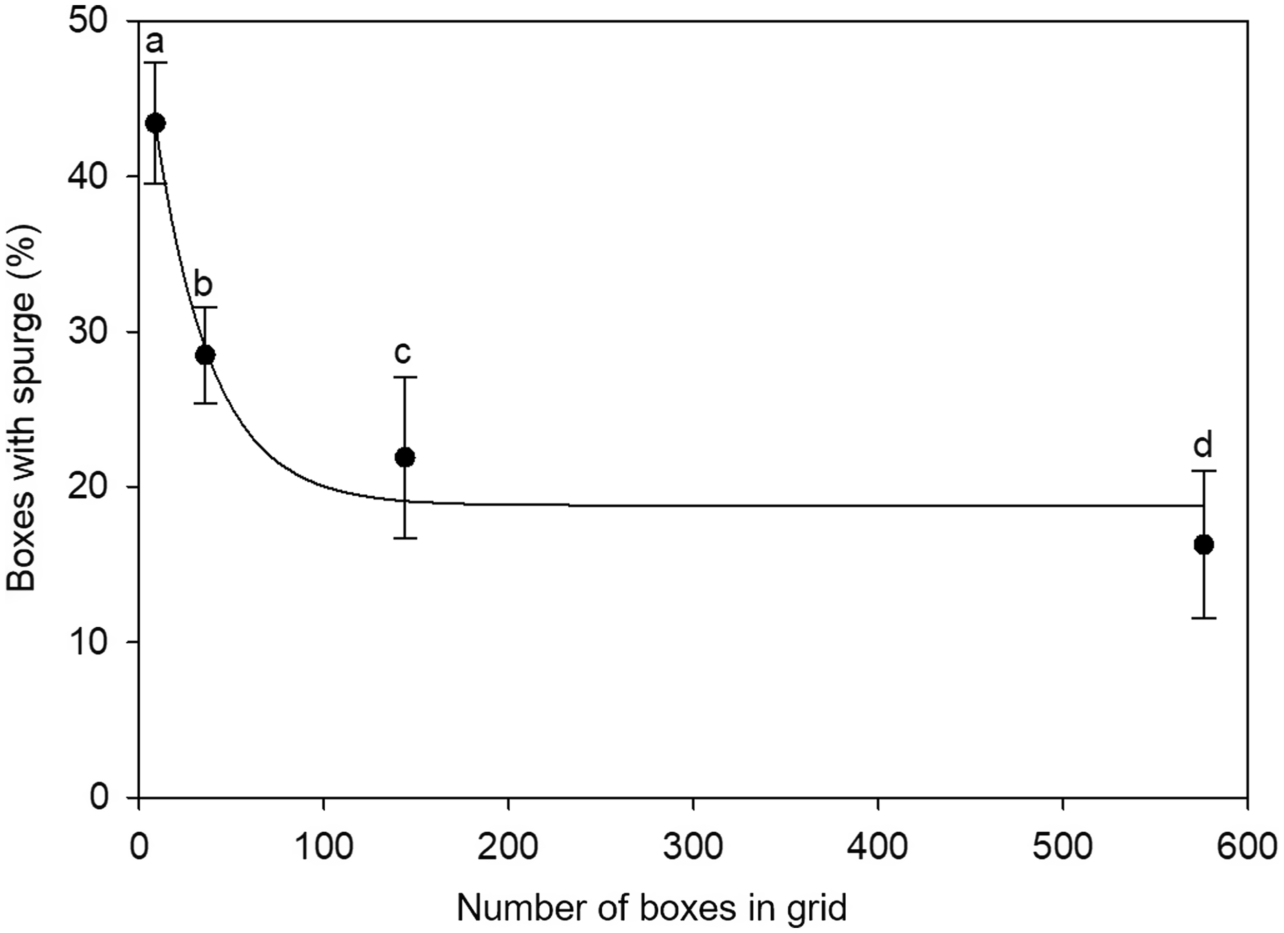
Figure 3. True infestation ratio, that is, the percentage of boxes containing spotted spurge regardless of detection (i.e., regardless, if labeled with bounding boxes; true infestation), at four box densities within a grid pattern. The error bars are the standard error of the mean (n = 50). Means marked with the same letter are not statistically different at P ≤ 0.05.

Figure 4. True hits ratio, that is, the percentage of boxes containing spotted spurge with labels only (true hits), at four box densities within a grid pattern. The error bars are the standard error of the mean (n = 50). Means marked with the same letter are not statistically different at P ≤ 0.05.

Figure 5. Misses ratio, that is, the percentage of boxes containing spotted spurge with no labels only (misses), at four box densities within a grid pattern. The error bars are the standard error of the mean (n = 50). Means marked with the same letter are not statistically different at P ≤ 0.05.

Figure 6. False hits ratio, that is, the percentage of boxes with labels devoid of spotted spurge (false hits), at four box densities within a grid pattern. The error bars are the standard error of the mean (n = 50). Means marked with the same letter are not statistically different at P ≤ 0.05.
Given the exponential nature of the data (Table 3), greater increases in efficiency were observed at lower nozzle densities. Conversely, diminishing returns occurred at higher nozzle densities, resulting in only slight improvements in ground cover accuracy when increasing from a 12 × 12 to a 24 × 24 grid. Thus, higher nozzle density provided better accuracy and greater herbicide reduction, which coincides with Rasmussen et al. (Reference Rasmussen, Azim, Nielsen, Mikkelsen, Hørfarter and Christensen2020). Moreover, Villette et al. (Reference Villette, Maillot, Guillemin and Douzals2021) concluded that in the case of small patches dispersed across the field, either independently operated nozzles or narrow boom sections are necessary to attain significant herbicide reduction.
Table 3. Evaluation and regression analysis for exponential decay models fit for four YOLO model performance metrics (true infestation ratio, true hits ratio, misses ratio, and false hits ratio), where the YOLO model was used for spotted spurge infestation detection on bermudagrass turf maintained as a golf course fairway
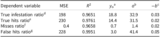
a Starting point of exponential decay models.
b Scaling factor.
c Rate of decay at box x.
d Percentage of grid boxes containing spurge regardless of detection (i.e., regardless, if labeled with bounding boxes; true infestation) to all boxes in the grid.
e Percentage of grid boxes containing bounding box–labeled (i.e., detected) spurge only (true hits) to all boxes in the grid.
f Percentage of grid boxes with spurge that was not labeled with bounding boxes (misses) to boxes containing spurge regardless of detection (i.e., regardless, if labeled with bounding boxes; true infestation).
g Percentage of grid boxes containing bounding box labels devoid of spurge (false hits) to all boxes in the grid.
The imagery data for this study were collected from areas representing high levels of weed infestation (i.e., ranging from 20% to 80% weed cover) forming relatively large mats. Weed distribution patterns under real-world scenarios may be less dense, forcing turfgrass managers to target smaller-sized individual plants. In such conditions, the accuracy of the spraying section, that is, higher nozzle density, gains importance. In this study, the difference in savings offered by the 12- and 24-nozzle scenarios was not statistically significant (Figure 4). However, the increase in the number of nozzles on the spraying section increases equipment and maintenance costs. On the basis of the results, optimal herbicide savings would occur with 12 nozzles applying a 4.17-cm band. Turfgrass is characterized by a low-mowed and uniform-height surface. To achieve such narrow bandwidth in those conditions, nozzle parameters like orifice size and distribution angle will need to be considered when developing booms and sprayers for targeted applications in such settings. Factors like boom height and turfgrass surface topography will also play important roles. Regardless, spray deposition uniformity within the bandwidth with minimal overlap is key to maintaining good coverage while ensuring the goal of maximizing efficiency. Achieving such objectives, along with verifying cost–benefit relationships of added costs and maintenance (an increased number of nozzles and valve actuators) versus herbicide cost savings will be a subject of future research with prototype sprayers.
Practical Implications
Overall, the results of this research bring the possibility of implementing modern targeted spraying technology closer to the turfgrass industry. This study confirms that object detection algorithms like YOLO can be successfully utilized for weed detection in developing targeted sprayers dedicated to turfgrass. The model developed in this study was able to differentiate structurally complex patches of weeds interwoven with turf, which are frequently observed under real-world conditions. This level of detection and distinction allows for targeted weed application and avoidance of the desired turf. Future research will focus on improving current CNN models’ efficacy, enhancing the training procedure, testing new algorithms, and broadening the spectrum of weed detection to include other species.
Despite a highly accurate weed detection system, precise herbicide application cannot be accomplished without precise and targeted spray delivery mechanisms. Owing to the precise nature of the differentiated detection, the area to be sprayed can be very limited. As such, the area covered by the nozzle should be correspondingly small, but the logistics in increasing nozzle density with ever-decreasing bandwidth is a major issue. Our research suggests that the 12-nozzle setting covering a 50-cm bandwidth (12 nozzles at 4.17-cm spacing) provides the optimal actuator accuracy with minimal financial outlay and results in ∼80% herbicide savings compared to broadcast application. Further research in this area should investigate the validity of these results under field conditions. Collectively, these results provide groundwork for further research and development of precision targeted spraying in turfgrass.
Acknowledgments
This work was supported by the USDA National Institute of Food and Agriculture, Research Capacity Funds (Hatch) FLA-AGR-006207, to the Agronomy Department, University of Florida, and FLA-FTL-005959, to the Fort Lauderdale Research and Education Center, University of Florida. The authors declare no conflicts of interest.


 Open access