


The importance of body composition in health and disease is well established(Reference Gupta, Lanca and Gan1–Reference Zong, Zhang and Yang4). However, contemporary methods of body composition estimation vary widely in their precision, accuracy and overall utility(Reference Ward5). The variable performance of techniques is confounded by dissimilarities in ‘reference’ methods and differing interpretations of acceptable agreement. Indeed, the utilisation of dual-energy X-ray absorptiometry (DXA) and other non-criterion laboratory methods for validation or calibration of simpler body composition methods has been identified as a noteworthy challenge to the clear establishment of acceptable whole-body methods(Reference Heymsfield, Ebbeling and Zheng6,Reference Wang, Deurenberg and Guo7) . However, while some methodological questions remain unresolved, a relative consensus exists that multi-component models are true in vivo reference methods for estimation of total body composition at the molecular level(Reference Heymsfield, Ebbeling and Zheng6,Reference Wang, Pi-Sunyer and Kotler8) .
Molecular-level multi-component models (i.e. multi-compartment models) separate all body mass (BM) into three or more components and typically require assessments using multiple laboratory techniques. Using specific input variables, most commonly the mass, volume, water content and bone mineral of the body, whole-body fat and fat-free mass (FFM) can be estimated using validated equations(Reference Heymsfield, Ebbeling and Zheng6). Several decades ago, it was established that multi-component models containing estimates of the body’s mass, volume and water content demonstrated the highest validity as compared with a criterion six-compartment model produced independently using in vivo neutron activation analysis(Reference Wang, Deurenberg and Guo7). Consequently, based on the inaccessibility of neutron activation facilities, it was suggested that the validated molecular-level multi-component models be used as reference methods in future work(Reference Heymsfield, Ebbeling and Zheng6,Reference Wang, Deurenberg and Guo7,Reference Heymsfield, Lichtman and Baumgartner9) . While some investigations have appropriately employed these models as reference methods, many contemporary technologies have limited or no validity data using a multi-component model reference method(Reference Ward5,Reference Heymsfield, Ebbeling and Zheng6,Reference Toombs, Ducher and Shepherd10) .
Traditionally, the utilisation of multi-component models has been limited by the requisite time, expense and expertise. However, two developments have increased the accessibility of these models. First, the validation of specific bioimpedance techniques against dilution reference methods for the estimation of total body water (TBW) has allowed for removal of the most time-intensive component of traditional multi-component models(Reference Earthman, Traughber and Dobratz11–Reference Armstrong, Kenefick and Castellani15). More recently, the utilisation of DXA-derived body volumes (BV) has allowed for a ‘rapid’ four-component (4C) model using only BM estimates, a DXA scan and a simple bioelectrical impedance assessment(Reference Smith-Ryan, Mock and Ryan16–Reference Wilson, Strauss and Fan18). While the utilisation of bioimpedance techniques is generally viewed as acceptable, particularly given the grossly disparate time required for assessment of TBW via dilution (hours for collection, followed by subsequent laboratory analysis) as compared with bioimpedance (minutes, with data immediately available), the utilisation of DXA-derived BV is less established, although a growing number of researchers have examined its use within a rapid 4C model(Reference Smith-Ryan, Mock and Ryan16–Reference Tinsley23).
While several common body composition assessment techniques have been evaluated in comparison with multi-component models(Reference Toombs, Ducher and Shepherd10,Reference Kyle, Bosaeus and De Lorenzo13,Reference Fields, Goran and McCrory24,Reference Friedl25) , the wide heterogeneity of specific devices and persistent technological improvement necessitate continued investigation of these frequently employed methods. Based on the continued need for multi-component model validation of laboratory and field body composition assessment techniques, the purpose of the present investigation was to determine the validity of body fat percentage (BF%) estimates from a variety of commonly employed methods, ranging from simple anthropometric equations to modified multi-component models, as compared with a five-component (5C) model criterion. BF% was selected as the body composition outcome of interest due to its applicability across the full spectrum of body sizes.
Methods
Overview
After an overnight food and fluid fast, 170 healthy adults were assessed by DXA, air displacement plethysmography (ADP), bioimpedance spectroscopy (BIS), multi-frequency bioelectrical impedance analysis (MFBIA), single-frequency bioelectrical impedance analysis (SFBIA) and three-dimensional optical scanning. In addition to providing BF% estimates, output from these techniques was used to produce a reference 5C model and multiple variants of 4C and three-component (3C) models. Circumferences from optical scanning were used in anthropometric BF% equations from the USA Department of Defense (DoD) as well as newer equations developed using National Health and Nutrition Examination Survey (NHANES) data. All BF% estimates were compared with the 5C model, and relevant group- and individual-level error metrics were generated.
Participants
Adults from the general population were recruited for participation. Prospective participants were excluded if they were <18 or >75 years of age, weighed >159 kg or were >193 cm in height (due to limitations of the DXA scanner), were missing any limbs or parts of limbs, had a pacemaker or electrical implant, had implanted metal due to prior medical procedure, were currently pregnant or trying to become pregnant or had previously undergone a body-altering surgery (e.g. breast augmentation, liposuction). One hundred and seventy participants completed the study and were included in the present analysis (Table 1). This study was conducted according to the guidelines laid down in the Declaration of Helsinki, and all procedures involving human participants were approved by the Texas Tech University institutional review board (IRB2018-417). Written informed consent was obtained from all participants.
Table 1. Participant characteristics
(Mean values and standard deviations; numbers)
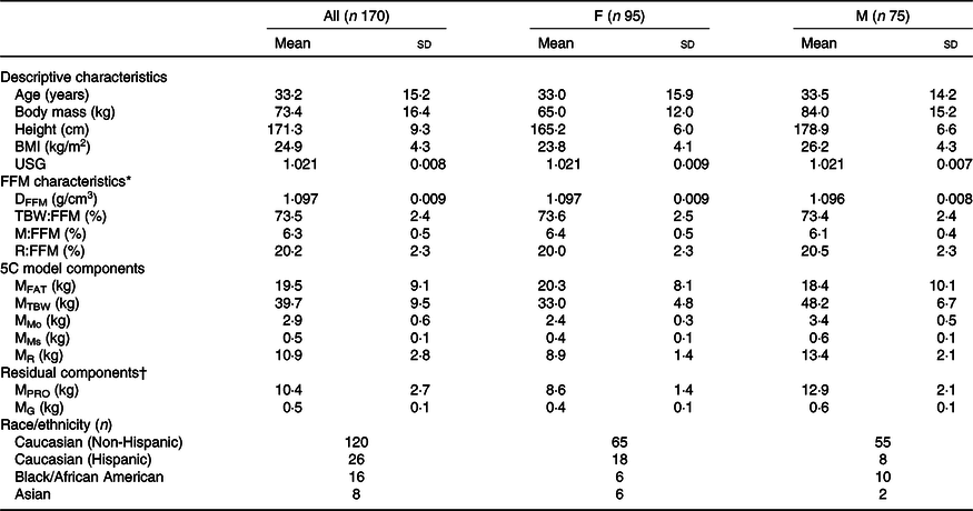
F, female; M, male; USG, urine specific gravity; FFM, fat-free mass; DFFM, density of fat-free mass; TBW:FFM, total body water to fat-free mass ratio; M:FFM, mineral (Mo + Ms) to fat-free mass ratio; R:FFM, residual to fat-free mass ratio; 5C, five-component model; MFAT, fat mass; MTBW, total body water mass; MMo, bone mineral mass; MMs, soft tissue mineral mass; MR, residual (protein + glycogen) mass; MPRO, protein mass; MG, glycogen mass.
* Reference values based on direct cadaver analysis are(Reference Wang, Heshka and Wang52): DFFM = 1·099 (sd 0·015); TBW:FFM = 73·7 (sd 3·8) %; M:FFM = 6·6 (sd 0·8) %; R:FFM = 19·7 (sd 3·2) %.
† Residual mass (MR) can further be divided into protein mass (MPRO) and glycogen mass (MG) in order to generate a six-component model using the assumption that MR = MPRO + MG, alongside the equation of Wang as presented by Heymsfield(Reference Heymsfield, Ebbeling and Zheng6): MG = 0·044 × MPRO.
Laboratory assessments
Initial procedures
Participants reported to the laboratory wearing light athletic clothing after overnight (≥8 h) abstention from eating, drinking, exercising and ingesting alcohol or caffeine. Adherence to these procedures was confirmed via interview. Prior to testing, all metal and accessories were removed, and each participant voided his or her bladder. Urine samples were collected, and urine specific gravity was assessed using a digital refractometer (PA201X-093, Misco). Equipment was calibrated as recommended by device manufacturers each day prior to use.
Dual-energy X-ray absorptiometry
DXA scans were performed on a Lunar Prodigy scanner (General Electric) with enCORE software (version 16.2). The scanner was calibrated daily prior to scanning using a manufacturer-supplied calibration block. Positioning of participants took place using custom-made foam blocks in order to promote consistency of positioning(Reference Nana, Slater and Hopkins26,Reference Moore, Benavides and Dellinger27) . Foam blocks were placed bilaterally between the hands and hips, with the hands placed in a neutral position. A block and strap at the feet ensured consistent foot positioning and orientation of the feet perpendicular to the scanning table. In the event that a participant was too broad to fit within DXA’s scanning dimensions, excluded body portions were estimated via reflection scanning techniques, which introduce minimal error(Reference Tinsley, Moore and Graybeal28,Reference Hangartner, Warner and Braillon29) . A trained operator manually adjusted region of interest lines within the enCORE software to specify body segments (i.e. arms, trunk and legs). DXA estimates of tissue and region BF% were obtained. DXA bone mineral content was multiplied by 1·0436 to yield an estimate of bone mineral (Mo)(Reference Heymsfield, Ebbeling and Zheng6,Reference Wang, Deurenberg and Guo7) . DXA estimates of lean soft tissue, fat mass and bone mineral content were also utilised to predict an additional BV estimate for use in a rapid 4C model using equation (1), which was developed by Wilson et al. (Reference Wilson, Strauss and Fan18) for GE DXA scanners:
 $${\rm{BV}}\left( {\rm{L}} \right) = {\rm}0\cdot933 \times {\rm{LST\;}} + {\rm{\;}}1\cdot150 \times {\rm{FM\;}} + {\rm{\;}} - \!0\cdot438 \times {\rm{BMC\;}} + {\rm{\;}}1\cdot504$$
Air displacement plethysmography
ADP (BOD POD®, Cosmed USA) was performed according to manufacturer recommendations and included two to three volume measurements to ensure consistent values. Measured thoracic gas volumes were used. ADP has previously demonstrated similar body density (D b) values to hydrostatic weighing and is considered a valid volumetric estimation technique for use in multi-component models(Reference Fields, Goran and McCrory24,Reference Millard-Stafford, Collins and Evans30,Reference Fields, Wilson and Gladden31) . Additionally, BF% estimates were obtained from ADP using the Siri(Reference Siri32) (equation (2)) and Brozek(Reference Brozek, Grande and Anderson33) (equation (3)) equations:
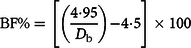 $${\rm{BF}}\% = \left[ {\left( {{{4\cdot95} \over {{D_{\rm{b}}}}}} \right) - 4\cdot5} \right] \times 100$$
 $${\rm{BF}}\% = {\rm{ }}\left[ {\left( {{{4\cdot57} \over {{D_{\rm{b}}}}}} \right) - 4\cdot142} \right] \times 100$$
The same D b value was used in both equations to yield two separate ADP BF% estimates for all participants, with the exception of Black/African American males (n 10) and females (n 6), who were evaluated using the equations of Schutte(Reference Schutte, Townsend and Hugg34) and Ortiz(Reference Ortiz, Russell and Daley35), respectively, as recommended by the manufacturer. For these individuals, the estimates obtained by the Schutte and Ortiz equations were used for both ADP BF% estimates. However, for conciseness, the ADP BF% estimates in this investigation are referred to as ‘Siri’ and ‘Brozek’ since the large majority of individuals (>90 %) were assessed using these equations.
Bioimpedance spectroscopy
BIS (SFB7, ImpediMed) was utilised to obtain TBW estimates using the manufacturer-specified hand-to-foot electrode arrangement. Each participant remained supine for ≥3 min immediately prior to BIS assessment. Coefficients utilised for males (ρ e = 273·9, ρ i = 937·2) and females (ρ e = 235·5, ρ i = 894·2), as well as body density, body proportion and hydration values (1·05, 4·30 and 0·732, respectively) were the same as those utilised in previous investigations with the selected BIS analyser(Reference Moon, Tobkin and Roberts36–Reference Tinsley, Moore and Benavides38). The BIS analyser used in the present study has previously been validated against deuterium dilution(Reference Moon, Tobkin and Roberts36,Reference Moon, Smith and Tobkin37) and obtains TBW estimates through Cole modelling(Reference Cole39) and mixture theories(Reference Hanai40) rather than regression equations used by the majority of bioimpedance methods (e.g. BIA)(Reference Kyle, Bosaeus and De Lorenzo12). BIS TBW volume estimates have compared favourably with dilution techniques in prior validation work(Reference Buendia, Seoane and Lindecrantz14,Reference Armstrong, Kenefick and Castellani15) . In the present study, assessments were conducted in duplicate and averaged for analysis. BIS output was reviewed for quality assurance through visual inspection of Cole plots. BIS TBW was also utilised for prediction of soft tissue mineral (Ms) using equation (4), which was developed by Wang et al. (Reference Wang, Xavier and Kotler41) using delayed-ϒ in vivo neutron activation:
 $${{\rm{M}}_{\rm{S}}} = 0\cdot882 \times \left( {12\cdot9 \times {\rm{TBW}}} \right) + 37\cdot9$$
Multi-frequency bioelectrical impedance analysis
Multi-frequency bioelectrical impedance analysis was performed using a 19-frequency, eight-point device (mBCA 515/514, Seca® GmbH & Co.) with contact electrodes and assessments conducted in the standing position. This analyser utilises frequencies ranging from 1 to 1000 kHz, a measuring current of 100 µA and has previously been validated against a 4C model for body composition estimates(Reference Bosy-Westphal, Schautz and Later42,43) . Assessments were conducted in duplicate and averaged for analysis.
Single-frequency bioelectrical impedance analysis
The SFBIA analyser (Quantum V, RJL Systems) was tested daily before any measurements using a manufacturer-supplied testing cell. Participant assessments were performed after approximately 5 min of supine rest. The SFBIA analyser employed an eight-point, bilateral, hand-to-foot electrode configuration. Electrode sites on the hand/wrist and foot/ankle were cleaned with alcohol pads prior to placement of the manufacturer-supplied adhesive electrodes. Electrodes were placed on the dorsal surfaces of both hands and both feet according to manufacturer specifications. Prior to assessment, each participant’s limbs were spread apart to ensure that they did not contact other body regions. Participants remained motionless in the supine position during assessments, and bioelectrical output was processed using manufacturer-provided software (RJL BC Segmental version 1.1.2). Assessments were conducted in duplicate and averaged for analysis.
Three-dimensional optical imaging
Three-dimensional optical imaging was performed using a structured light scanner with static components (Size Stream® SS20; scanner version 6.0.0.32)(Reference Tinsley, Moore and Dellinger44). This scanner utilises a reference object, in the form of a hanging panel with checkerboard pattern, for sensor calibration prior to scanning. The calibration procedure was completed daily prior to scanning. Participants wore minimal form-fitting clothing during assessments. Scans were conducted in duplicate using a five-scan multi-scan mode and averaged for analysis. Scans were processed using Size Stream Studio software version 5.2.7 to obtain height and circumference estimates used in the anthropometric BF% equations. The root mean square coefficient of variation and intraclass correlation coefficient for height estimates in our laboratory, using the three-dimensional optical scanner, are 0·22 and 0·998 %, respectively. The reliability of other anthropometric estimates from this scanner has previously been reported(Reference Tinsley, Moore and Dellinger44).
Multi-component models
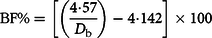
The criterion estimate of body composition was obtained from a 5C model (Table 2). In this model, BV was obtained from ADP, Mo from DXA and TBW and Ms from BIS. The BM estimate was obtained from the calibrated scale associated with the ADP device.
Table 2. Description of body composition models
BM, body mass; BV, body volume; TBW, total body water; Mo, bone mineral; Ms, soft tissue mineral; 5C, five-component model; CS, calibrated scale; ADP, air displacement plethysmography; BIS, bioimpedance spectroscopy; DXA, dual-energy X-ray absorptiometry; 4C, four-component model; MFBIA, multi-frequency bioelectrical impedance analysis; SFBIA, single-frequency bioelectrical impedance analysis; 3C, three-component model; REG, region; TISS, tissue; BROZEK, Brozek(Reference Brozek, Grande and Anderson33) two-component model body fat equation; SIRI, Siri(Reference Siri32) two-component model body fat equation; S, scale built into MFBIA analyzer; DoD, Department of Defense body fat equation(48); LEE, Lee et al. (Reference Lee, Keum and Hu49) body fat equations.
The equation of Wang et al. (Reference Wang, Xavier and Kotler41) (equation (5)) was utilised for estimation of 5C BF%:
 $$\displaylines{
{\rm{BF}}\% \; = 100 \cr
\times {{2\cdot748 \times {\rm{BV}}\; - \;0\cdot715 \times {\rm{TBW}}\; + \;1\cdot129 \times {\rm{Mo}} + 1\cdot222 \times {{\rm{M}}_{\rm{S}}}\; - \;2\cdot051 \times {\rm{BM}}} \over {{\rm{BM}}}} \cr} $$
$$\displaylines{
{\rm{BF}}\% \; = 100 \cr
\times {{2\cdot748 \times {\rm{BV}}\; - \;0\cdot715 \times {\rm{TBW}}\; + \;1\cdot129 \times {\rm{Mo}} + 1\cdot222 \times {{\rm{M}}_{\rm{S}}}\; - \;2\cdot051 \times {\rm{BM}}} \over {{\rm{BM}}}} \cr} $$
Additional multi-component models estimates were produced. The Wang et al. (Reference Wang, Xavier and Kotler41) 4C estimate was produced using equation (6):
 $${\rm{BF}}\% = 100 \times {\rm{ }}{{2\cdot748 \times {\rm{BV}}\; - \;0\cdot699 \times {\rm{TBW}}\; + \;1\cdot129 \times {\rm{Mo}}\; - \;2\cdot051 \times {\rm{BM}}} \over {{\rm{BM}}}}$$
Versions of the Wang et al. 4C model were produced using BIS, multi-frequency bioelectrical impedance analysis and SFBIA TBW estimates. An additional model, the rapid 4C model, was produced using the DXA-derived BV estimate.
The Siri three-compartment (3C) model was calculated using equation (7), as presented in Siri(Reference Siri, Henschel and Brožek45):
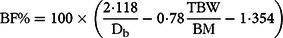 $${\rm{BF}}\% = 100 \times {\rm{ }}\left( {{{2\cdot118} \over {{{\rm{D}}_{\rm{b}}}}} - {\rm{ }}0\cdot78\,{{{\rm{TBW}}} \over {{\rm{BM}}}} - 1\cdot354} \right)$$
D b estimates were obtained from ADP, and BIS TBW was used. Alternate versions of the Siri 3C model were produced using multi-frequency bioelectrical impedance analysis and SFBIA TBW.
Additionally, the Lohman 3C model(Reference Lohman46), which includes an estimate of total body mineral (M; equivalent to Mo × 1·235(Reference Moon, Eckerson and Tobkin47)), was calculated using equation (8):
 $${\rm{BF}}\% = 100 \times {\rm{ }}{{6\cdot386 \times {\rm{BV}} + 3\cdot96 \times {\rm{M}} - 6\cdot09 \times {\rm{BM}}} \over {{\rm{BM}}}}$$
Anthropometric body composition equations
Anthropometric BF% estimations were calculated using the Department of Defense (DoD)/army body fat equations(48), and three equations developed using National Health and Nutrition Examination Survey (NHANES) data by Lee et al. (Reference Lee, Keum and Hu49). These equations were developed using manual circumferences obtained with a tape measure. In the present investigation, the anthropometric estimates from three-dimensional optical imaging were utilised(Reference Tinsley, Moore and Dellinger44). Previous research has indicated that circumference estimates obtained by three-dimensional optical scanning may exhibit either slightly superior(Reference Medina-Inojosa, Somers and Ngwa50) or inferior(Reference Bourgeois, Ng and Latimer51) reliability as compared with manual estimates, which may depend on the expertise of the manual assessor.
The DoD BF% equations for females (equation (9)) and males (equation (10) are(48)
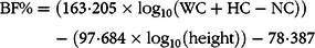 $$\displaylines{
{\rm{BF}}\% = \left( {163\cdot205 \times {\rm{lo}}{{\rm{g}}_{10}}\left( {{\rm{WC}} + {\rm{HC}} - {\rm{NC}}} \right)} \right) \cr
- \left( {97\cdot684 \times {\rm{lo}}{{\rm{g}}_{10}}\left( {{\rm{height}}} \right)} \right) - 78\cdot387 \cr} $$
$$\displaylines{
{\rm{BF}}\% = \left( {163\cdot205 \times {\rm{lo}}{{\rm{g}}_{10}}\left( {{\rm{WC}} + {\rm{HC}} - {\rm{NC}}} \right)} \right) \cr
- \left( {97\cdot684 \times {\rm{lo}}{{\rm{g}}_{10}}\left( {{\rm{height}}} \right)} \right) - 78\cdot387 \cr} $$
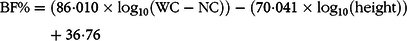 $$\displaylines{
{\rm{BF}}\% = \left( {86\cdot010 \times {\rm{lo}}{{\rm{g}}_{10}}\left( {{\rm{WC}} - {\rm{NC}}} \right)} \right) - \left( {70\cdot041 \times {\rm{lo}}{{\rm{g}}_{10}}\left( {{\rm{height}}} \right)} \right) \cr
+ 36\cdot76 \cr} $$
$$\displaylines{
{\rm{BF}}\% = \left( {86\cdot010 \times {\rm{lo}}{{\rm{g}}_{10}}\left( {{\rm{WC}} - {\rm{NC}}} \right)} \right) - \left( {70\cdot041 \times {\rm{lo}}{{\rm{g}}_{10}}\left( {{\rm{height}}} \right)} \right) \cr
+ 36\cdot76 \cr} $$
In these equations, WC refers to waist circumference, HC is hip circumference and NC is neck circumference, with all values entered in inches.
Several progressively more complex equations were produced from NHANES data by Lee et al. (Reference Lee, Keum and Hu49). For equations (11–16), additional terms for race/ethnicity adjustments were included using the appropriate coefficients presented in Table 2 of Lee et al. (Reference Lee, Keum and Hu49). For females, the equations developed by Lee et al., which correspond to equations 1–3 in the original report(Reference Lee, Keum and Hu49), are
 $${\rm{BF\% }} = 58\cdot60 + 0\cdot08 \times {\rm{age}} - 0\cdot30 \times {\rm{height}} + 0\cdot35 \times {\rm{BM}}$$
 $$\displaylines{
{\rm{BF}}\% = 50\cdot46 + 0\cdot07 \times {\rm{age}} - 0\cdot26 \times {\rm{height}} + 0\cdot27 \times {\rm{BM}} \cr
+ 0\cdot10 \times {\rm{WC}} \cr} $$
$$\displaylines{
{\rm{BF}}\% = 50\cdot46 + 0\cdot07 \times {\rm{age}} - 0\cdot26 \times {\rm{height}} + 0\cdot27 \times {\rm{BM}} \cr
+ 0\cdot10 \times {\rm{WC}} \cr} $$
 $$\displaylines{
{\rm{BF}}\% = 27\cdot57 + 0\cdot08 \times {\rm{age}} - 0\cdot17 \times {\rm{height}} + 0\cdot09 \times {\rm{BM}} \cr
+ 0\cdot14 \times {\rm{WC}} + 0\cdot27 \times {\rm{AC}} - 0\cdot18 \times {\rm{CC}} + 0\cdot29 \times {\rm{TC}} \cr} $$
$$\displaylines{
{\rm{BF}}\% = 27\cdot57 + 0\cdot08 \times {\rm{age}} - 0\cdot17 \times {\rm{height}} + 0\cdot09 \times {\rm{BM}} \cr
+ 0\cdot14 \times {\rm{WC}} + 0\cdot27 \times {\rm{AC}} - 0\cdot18 \times {\rm{CC}} + 0\cdot29 \times {\rm{TC}} \cr} $$
Units of years are used for age, kg for BM, and cm for height, WC, arm circumference (AC), calf circumference (CC) and thigh circumference (TC).
For males, the equations developed by Lee et al., which correspond to equations 1–3 in the original report(Reference Lee, Keum and Hu49), are
 $${\rm{BF\% }} = 44\cdot47 + 0\cdot10 \times {\rm{age}} - 0\cdot26 \times {\rm{height}} + 0\cdot29 \times {\rm{BM}}$$
 $$\displaylines{
{\rm{BF}}\% = 0\cdot02 + 0\cdot00 \times {\rm{age}} - 0\cdot07 \times {\rm{height}} - 0\cdot08 \times {\rm{BM}} + 0\cdot48 \cr
\times {\rm{WC}} \cr} $$
$$\displaylines{
{\rm{BF}}\% = 0\cdot02 + 0\cdot00 \times {\rm{age}} - 0\cdot07 \times {\rm{height}} - 0\cdot08 \times {\rm{BM}} + 0\cdot48 \cr
\times {\rm{WC}} \cr} $$
 $$\displaylines{
{\rm{BF}}\% = - 3\cdot10 + 0\cdot01 \times {\rm{age}} - 0\cdot06 \times {\rm{height}} - 0\cdot10 \times {\rm{BM}} + 0\cdot49 \cr
\times {\rm{WC}} - 0\cdot09 \times {\rm{AC}} - 0\cdot02 \times {\rm{CC}} + 0\cdot12 \times {\rm{TC}} \cr} $$
$$\displaylines{
{\rm{BF}}\% = - 3\cdot10 + 0\cdot01 \times {\rm{age}} - 0\cdot06 \times {\rm{height}} - 0\cdot10 \times {\rm{BM}} + 0\cdot49 \cr
\times {\rm{WC}} - 0\cdot09 \times {\rm{AC}} - 0\cdot02 \times {\rm{CC}} + 0\cdot12 \times {\rm{TC}} \cr} $$
Fat-free mass characteristics
To provide a comprehensive examination of participant characteristics (Table 1) and confirm similarity with reference values, FFM characteristics were estimated using data from the aforementioned laboratory procedures. These characteristics included the density of FFM (DFFM) and proportions of TBW, mineral (i.e. Mo + Ms) and residual (i.e. protein and glycogen) in FFM, designated as TBW:FFM, M:FFM and R:FFM. Residual content (R) was calculated by subtraction using equation (17), with FM5C representing the 5C model FM estimate:
 $${\rm{R}} = {\rm{BM}} - {\rm{TBW}} - {\rm{Mo}} - {\rm{Ms}} - {\rm{F}}{{\rm{M}}_{5{\rm{C}}}}$$
DFFM, TBW:FFM, M:FFM, and F:FFM were calculated using equations (18–21), which are based on those presented by Wang et al. (Reference Wang, Heshka and Wang52):
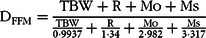 $${{\rm{D}}_{{\rm{FFM}}}} = {\rm{ }}{{{\rm{TBW}} + {\rm{R}} + {\rm{Mo}} + {\rm{Ms}}} \over {{{{\rm{TBW}}} \over {0\cdot9937}} + {\rm{ }}{{\rm{R}} \over {1\cdot34}} + {\rm{ }}{{{\rm{Mo}}} \over {2\cdot982}} + {\rm{ }}{{{\rm{Ms}}} \over {3\cdot317}}}}$$
 $${\rm{TBW}}:{\rm{FFM\;}} = {\rm{\;TBW}}/{\rm{FF}}{{\rm{M}}_{5{\rm{C\;}}}}$$
 $${\rm{M}}:{\rm{FFM\;}} = \left( {{\rm{Mo}} + {\rm{Ms}}} \right)/{\rm{FF}}{{\rm{M}}_{5{\rm{C\;}}}}$$
 $${\rm{R}}:{\rm{FFM\;}} = {\rm{\;R}}/{\rm{FF}}{{\rm{M}}_{5{\rm{C}}}}$$
Statistical analysis
Sample size was determined based on resource availability due to the exploratory nature of this analysis; however, the final sample size was comparable with or larger than many previous validation studies(Reference Toombs, Ducher and Shepherd10,Reference Kyle, Bosaeus and De Lorenzo13,Reference Fields, Goran and McCrory24) . Descriptive data for BF% estimates produced by each body composition model and method were generated (Table 3). The constant error (CE) was calculated as the mean difference between the 5C criterion and each alternate method (i.e. alternate estimate minus 5C estimate). Equivalence testing was used to evaluate whether each method demonstrated equivalence with the 5C model based on a 2 % equivalence region, and the 90 % confidence limits for the two-one-sided t tests were calculated(Reference Dixon, Saint-Maurice and Kim53). Null hypothesis significance testing (NHST) was also performed, and the 95 % confidence limits were calculated. The Pearson correlation coefficient (r) and coefficient of determination (R 2) were estimated. Ordinary least squares and Deming regressions were performed to compare the intercept and slope of regression lines to the line of identity (i.e. the perfect linear relationship between methods with an intercept of 0 and a slope of 1). In contrast to ordinary least squares regression, which is commonly implemented in methodological investigations, Deming regression accounts for error in the measurement of both x and y variables and thus may be more appropriate when errors are present for both criterion and comparison methods(Reference Therneau54). The standard error of the estimate (SEE; i.e. residual SE) was obtained from ordinary least squares regression. For both regression analyses, the 5C model was designated as the criterion variable (Y), and the alternate model was designated as the predictor variable (X). The subjective ranking categories of American College of Sports Medicine et al. (Reference Lohman and Milliken55) were utilised for categorisation of BF% SEE. The methods of Bland & Altman(Reference Bland and Altman56) were utilised alongside linear regression to assess the degree of proportional bias. The 95 % limits of agreement (LOA) were calculated. The total error (TE) (i.e. root mean square error or pure error) was calculated using equation (22):
 $${\rm{TE}} = {\rm{\;\;}}\sqrt {{\rm{ }}{{\left( {{\rm{BF}}{{\rm{\% }}_{{\rm{ALT}}}} - {\rm{BF}}{{\rm{\% }}_{5{\rm{C}}}}} \right)}^2}/n} {\rm{\;}}$$
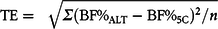
Table 3. Body composition estimates*
(Mean values and standard deviations; 95 % confidence intervals)
TOST, two one-sided test; CE, constant error; LL, lower limit of confidence interval; UL, upper limit of confidence interval; NHST, null hypothesis significance testing in the form of paired-samples t test. TE, total error; Equiv, equivalence testing result; SEE, standard error of the estimate; 5C, five-component model; 4C, four-component model; Y, yes, equivalent based on 2 % equivalence region; MFBIA, multi-frequency bioelectrical impedance analysis; SFBIA, single-frequency bioelectrical impedance analysis; DXA, dual-energy X-ray absorptiometry; N, no – not equivalent based on 2 % equivalence region; 3C, three-component model; REG, region; TISS, tissue; BROZEK, Brozek(Reference Brozek, Grande and Anderson33) two-component model body fat equation; SIRI, Siri(Reference Siri32) two-component model body fat equation; ADP, air displacement plethysmography; BIS, bioimpedance spectroscopy; DoD, Department of Defense body fat equation(48); LEE, Lee et al. (Reference Lee, Keum and Hu49) body fat equations.
† Based on subjective ranking categories of Lohman & Milliken(Reference Lohman and Milliken55).
where BF%ALT is the BF% estimate for the alternate body composition method in question. Data were analysed using R (version 3.6.1)(57). The primary packages utilised include psych (Reference Revelle58) , TOSTER (Reference Lakens59), deming (Reference Therneau54), DescTools (60) and ggplot2 (Reference Wickham61).
Results
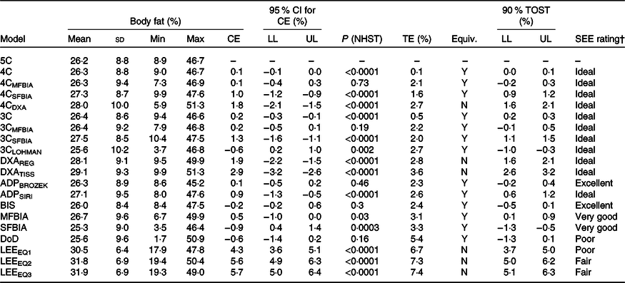
A broad summary of the performance of each method, including a comparison of CE, SEE and TE values, is displayed in Fig. 1.
Fig. 1. Overview of select validity metrics. The constant error (CE; body fat % (BF%) for alternate method minus BF% value for 5C model) is displayed in panel (a). The standard error of the estimate (SEE; deviation of individual data points around the regression line) is displayed in panel (b). The TE (i.e. root mean square error or pure error; average deviation of individual scores from the line of identity) is displayed in panel (c). For all panels, methods are sorted in order of increasing error. 4C, four-component model; 5C, five-component model; ADP, air displacement plethysmography; BIS, bioimpedance spectroscopy; BROZEK, Brozek(Reference Brozek, Grande and Anderson33) two-component model body fat equation; CE, constant error; DoD, Department of Defense body fat equation(48); DXA, dual-energy X-ray absorptiometry; LEE, Lee et al. (Reference Lee, Keum and Hu49) body fat equations; MFBIA, multi-frequency bioelectrical impedance analysis; SFBIA, single-frequency bioelectrical impedance analysis; SIRI, Siri(Reference Siri32) two-component model body fat equation.
Multi-component models
4C models exhibited CE values of 0·1– 1·8 % and TE values of 0·1–2·7 % (Table 3). R 2 values ranged from 0·95 to 1·00, with SEE values of 0·02–1·99 % (Fig. 2). LOA ranged from 0·04 to 4·16 %. All 4C models except 4CDXA demonstrated equivalence with 5C based on the 2 % equivalence interval.
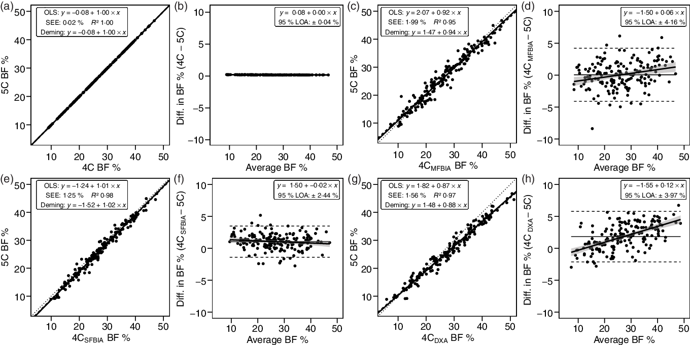
Fig. 2. Performance of four-component (4C) models. Validity analysis is displayed for 4C with BIS TBW estimates (a, b), 4C with multi-frequency BIA TBW estimates (c, d), 4C with SFBIA TBW estimates (e, f), and 4C with DXA-derived BV and BIS TBW estimates (g, h). The Wang et al. (Reference Wang, Pi-Sunyer and Kotler8) 4C equation was used for all models. Panels a, c, e and g depict ordinary least squares (OLS) regression lines (dashed) and Deming regression lines (solid) as compared with the line of identity (dotted). The standard error of the estimate (SEE) and coefficient of determination (R 2) are also displayed. Panels b, d, f and h depict Bland–Altman analysis, with the solid diagonal line representing the relationship between the difference in body composition estimates, calculated as the comparison method estimate minus the five-component (5C) estimate, and the average of comparison and 5C estimates. The shaded regions around the diagonal line indicate the 95 % confidence limits for the linear regression line, the horizontal dashed lines indicate the upper and lower limits of agreement (LOA), and the horizontal solid line indicates the constant error between methods. Linear regression equations and 95 % LOA values are also displayed. BIS, bioimpedance spectroscopy; TBW, total body water; SFBIA, single-frequency bioelectrical impedance analysis; DXA, dual-energy X-ray absorptiometry; BV, body volume; BF, body fat.
3C models exhibited CE values of −0·6 to 1·3 % and TE values of 0·5–2·7 %. R 2 values ranged from 0·94 to 1·00, with SEE values of 0·39–2·10 % (Fig. 3). LOA ranged from 0·87 to 5·24 %, and all 3C models demonstrated equivalence with 5C (Table 3).
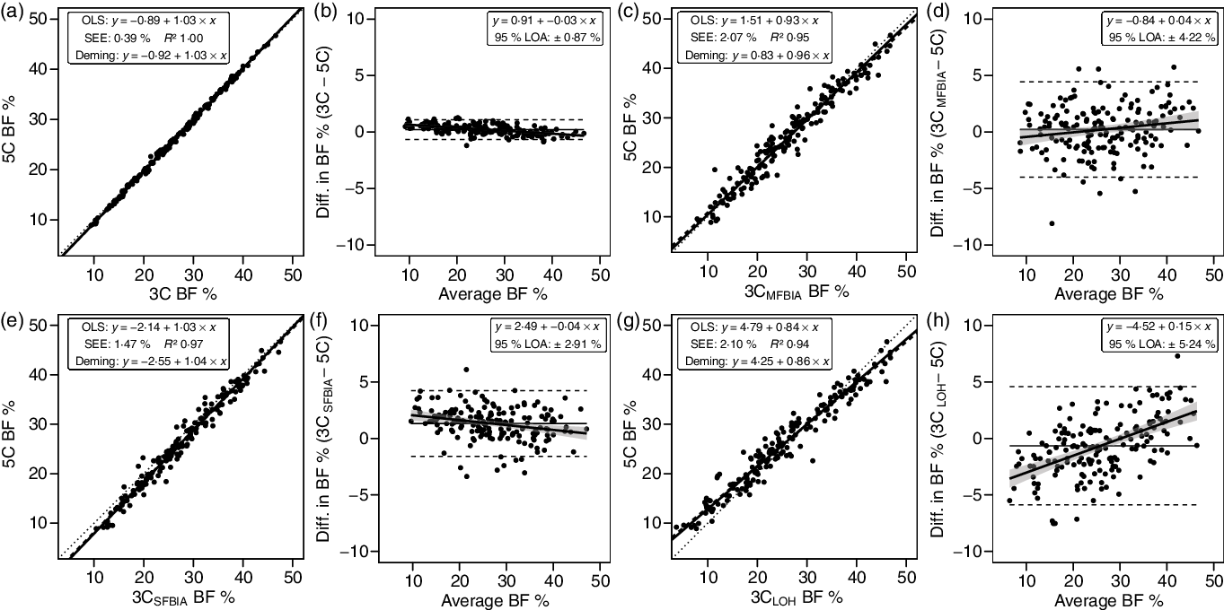
Fig. 3. Performance of three-component (3C) models. Validity analysis is displayed for Siri 3C model(Reference Siri, Henschel and Brožek45) with BIS TBW estimates (a, b), Siri 3C model with multi-frequency BIA TBW estimates (c, d), Siri 3C model with SFBIA TBW estimates (e, f), and Lohman 3C model(Reference Lohman46) (g, h). Panels a, c, e and g depict ordinary least squares (OLS) regression lines (dashed) and Deming regression lines (solid) as compared with the line of identity (dotted). The standard error of the estimate (SEE) and coefficient of determination (R 2) are also displayed. Panels b, d, f and h depict Bland–Altman analysis, with the solid diagonal line representing the relationship between the difference in body composition estimates, calculated as the comparison method estimate minus the five-component (5C) estimate, and the average of comparison and 5C estimates. The shaded regions around the diagonal line indicate the 95 % confidence limits for the linear regression line, the horizontal dashed lines indicate the upper and lower limits of agreement (LOA), and the horizontal solid line indicates the constant error between methods. Linear regression equations and 95 % LOA values are also displayed. BIS, bioimpedance spectroscopy; TBW, total body water; SFBIA, single-frequency bioelectrical impedance analysis; BF, body fat.
Laboratory methods
DXA BF% estimates exhibited CE values of 1·9–2·9 % and TE values of 2·8–3·6 % (Table 3). The R 2 value was 0·95 for both DXA BF% estimates, with SEE of approximately 2·1 % (Fig. 4). LOA ranged from 4·12 to 4·26 %, and neither DXA BF% estimate exhibited equivalence with 5C.
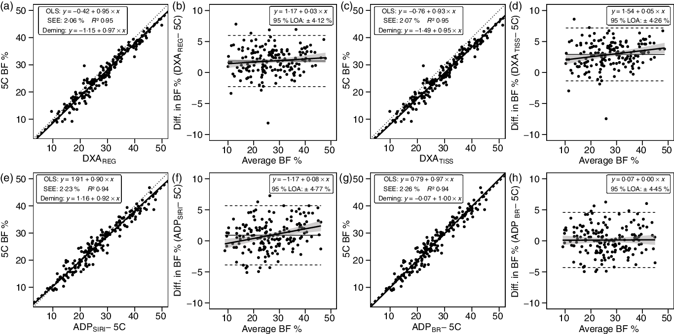
Fig. 4. Performance of dual-energy X-ray absorptiometry (DXA) and air displacement plethysmography (ADP). Validity analysis is displayed for DXA region body fat % (BF%) (a, b), DXA tissue BF% (c, d), ADP BF% with Siri equation(Reference Siri32) (e, f), and ADP BF% with Brozek equation(Reference Brozek, Grande and Anderson33) (g, h). Panels a, c, e and g depict ordinary least squares (OLS) regression lines (dashed) and Deming regression lines (solid) as compared with the line of identity (dotted). The standard error of the estimate (SEE) and coefficient of determination (R 2) are also displayed. Panels b, d, f and h depict Bland–Altman analysis, with the solid diagonal line representing the relationship between the difference in body composition estimates, calculated as the comparison method estimate minus the five-component (5C) estimate, and the average of comparison and 5C estimates. The shaded regions around the diagonal line indicate the 95 % confidence limits for the linear regression line, the horizontal dashed lines indicate the upper and lower limits of agreement (LOA), and the horizontal solid line indicates the constant error between methods. Linear regression equations and 95 % LOA values are also displayed.
ADP BF% estimates exhibited CE values of 0·1–0·9 % and TE values of 2·3–2·6 % (Table 3). The R 2 value was 0·94 for both ADP BF% estimates, with SEE of approximately 2·2 % (Fig. 4). LOA ranged from 4·45 to 4·77 %, and both ADP BF% estimates exhibited equivalence with 5C.
Field methods
Bioimpedance methods exhibited CE values of −0·9 to 0·5 % and TE values of 2·4–3·3 %. R 2 values ranged from 0·88 to 0·93, with SEE values of 2·36–3·09 % (Fig. 5). LOA ranged from 4·62 to 6·22 %, and all bioimpedance methods demonstrated equivalence with 5C (Table 3).
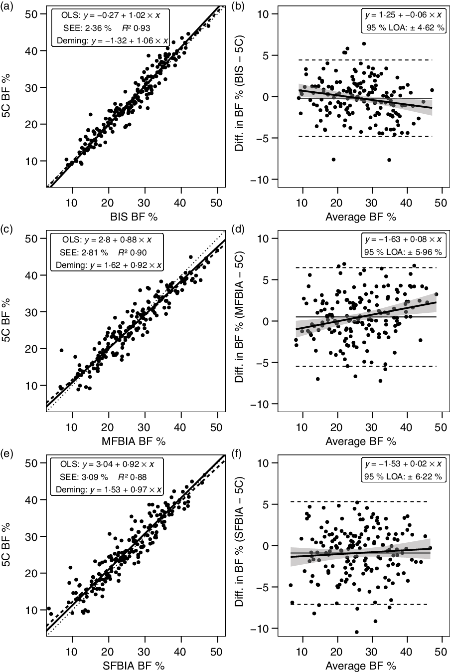
Fig. 5. Performance of bioimpedance techniques. Validity analysis is displayed for bioimpedance spectroscopy (BIS) (a, b), multi-frequency bioelectrical impedance analysis (MFBIA) (c, d), and single-frequency bioelectrical impedance analysis (SFBIA) (e, f). Panels a, c and e depict ordinary least squares (OLS) regression lines (dashed) and Deming regression lines (solid) as compared with the line of identity (dotted). The standard error of the estimate (SEE) and coefficient of determination (R 2) are also displayed. Panels b, d and f depict Bland–Altman analysis, with the solid diagonal line representing the relationship between the difference in body composition estimates, calculated as the comparison method estimate minus the five-component (5C) estimate, and the average of comparison and 5C estimates. The shaded regions around the diagonal line indicate the 95 % confidence limits for the linear regression line, the horizontal dashed lines indicate the upper and lower limits of agreement (LOA), and the horizontal solid line indicates the constant error between methods. Linear regression equations and 95 % LOA values are also displayed. BF, body fat.
Anthropometric methods exhibited CE values of −0·6 to 5·7 % and TE values of 5·4–7·4 %. R 2 values ranged from 0·67 to 0·73, with SEE values of 4·61–5·11 % (Fig. 6). LOA ranged from 9·10 to 10·56 %. Only the DoD BF% equation demonstrated equivalence with 5C (Table 3).
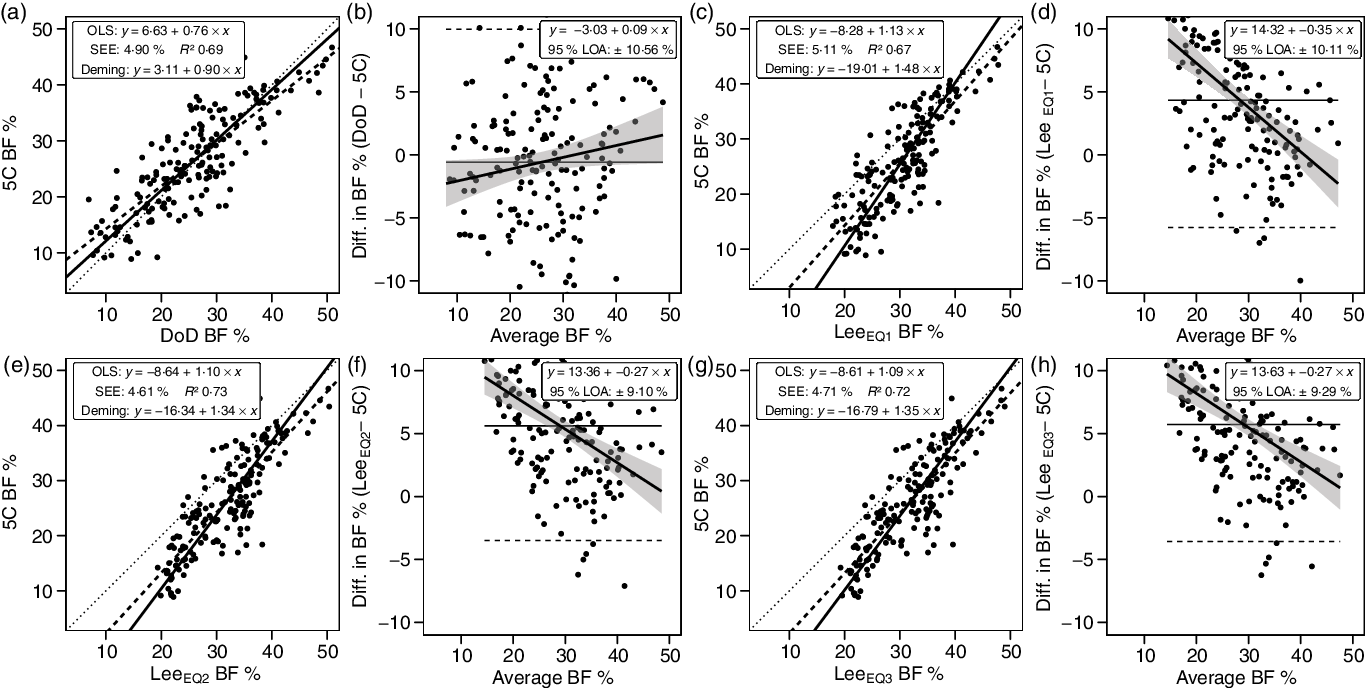
Fig. 6. Performance of anthropometric equations. Validity analysis is displayed for the Department of Defense (DoD) body fat % (BF%) equation(48) (a, b), Lee et al. (Reference Lee, Keum and Hu49) equation (1) (c, d), Lee et al. (Reference Lee, Keum and Hu49) equation (2) (e, f) and Lee et al. (Reference Lee, Keum and Hu49) equation (3) (g, h). Panels a, c, e and g depict ordinary least squares (OLS) regression lines (dashed) and Deming regression lines (solid) as compared with the line of identity (dotted). The standard error of the estimate (SEE) and coefficient of determination (R 2) are also displayed. Panels b, d, f and h depict Bland–Altman analysis, with the solid diagonal line representing the relationship between the difference in body composition estimates, calculated as the comparison method estimate minus the five-component (5C) estimate, and the average of comparison and 5C estimates. The shaded regions around the diagonal line indicate the 95 % confidence limits for the linear regression line, the horizontal dashed lines indicate the upper and lower limits of agreement (LOA) and the horizontal solid line indicates the constant error between methods. Linear regression equations and 95 % LOA values are also displayed.
Discussion
The purpose of the present investigation was to determine the validity of body composition estimates from a variety of commonly employed methods as compared with a 5C model criterion. Major findings were (1) differences between 5C, 4C and 3C models utilising the same BV and TBW estimates are negligible (CE ≤ 0·2 %; SEE < 0·5 %; TE ≤ 0·5 %; R 2 1·00; 95 % LOA ≤ 0·9 %), indicating that these models can be viewed interchangeably in many cases and that the utility of additional mineral estimates (i.e. bone mineral and soft tissue mineral) are questionable; (2) errors introduced by utilising alternate TBW (i.e. multi-frequency bioelectrical impedance analysis or SFBIA) or BV (i.e. DXA-derived) estimates are relatively small but would likely be meaningful in some contexts (CE ≤ 1·3 %; SEE ≤ 2·1 %; TE ≤ 2·2 %; R 2 ≥ 0·95; 95 % LOA ≤ 4·2 %); (3) small but potentially relevant differences between alternate DXA (i.e. tissue v. region) and ADP (i.e. Siri v. Brozek equations) BF% estimates were observed, and these techniques generally performed well (CE < 3·0 %; SEE: ≤ 2·3 %; TE ≤ 3·6 %; R 2 ≥ 0·88; 95 % LOA < 4·8 %); (4) bioimpedance technologies performed relatively well (CE < 1·0 %; SEE ≤ 3·1 %; TE ≤ 3·3 %; R 2 ≥ 0·94; 95 % LOA ≤ 6·2 %), although individual-level errors were generally larger than all other non-anthropometric methods and (5) newer anthropometric BF% equations produced using NHANES data did not outperform the DoD BF% equation and in fact exhibited much higher group-level error (DoD: CE = 0·6 %; NHANES: CE = 4·3–5·7 %); as expected, performance of anthropometric equations was relatively poor compared with other methods (SEE ≤ 5·1 %; TE ≤ 7·4 %; R 2 ≥ 0·67; 95 % LOA ≤ 10·6 %). Importantly, the context in which a method is utilised and the purpose of the assessment impact the interpretation of the observed errors. For example, while DXA demonstrated a statistically significant difference from 5C and lack of equivalence, both of which are group-level considerations, the SEE and 95 % LOA, both of which provide information regarding individual-level validity, indicated relatively low error.
In contrast to the present study, several prior validity examinations of DXA as compared with a multi-component model have indicated an underestimation of BF% by DXA at the group level(Reference Toombs, Ducher and Shepherd10). However, meaningful differences in DXA scanning and software technology limit the ability to compare results across studies with differing methodologies. In fact, although an earlier software version was used, prior research using the same DXA scanner as the present investigation (GE Lunar Prodigy) demonstrated overestimations of BF% relative to a 4C model that were very similar to those of the present study (1·7–2·3 v. 1·9 %)(Reference Williams, Wells and Wilson62). In the present analysis, it was also observed that the region BF% value, which is based on all observed pixels, exhibited slightly better agreement with 5C as compared with the tissue BF% value, which is based only on soft tissue pixels. The difference amounted to 1·0 % on average (CE of 1·9 v. 2·9 %) and resulted in a better TE value for DXAREGION as compared with DXATISSUE (2·8 v. 3·6 %). The closer agreement of the region BF% value is reasonable based on the fact that bone mineral is included in both the 5C and DXAREGION, but not DXATISSUE. Based on examination of publicly available NHANES data, it was confirmed that the NHANES dataset, and therefore published reference values from this dataset(Reference Kelly, Wilson and Heymsfield63), utilise region BF%. Based on calculation, the mean difference between region and tissue BF% in the 1999–2004 NHANES dataset is 1·0 (sd 0·2) %, with a higher estimate for tissue BF%. This difference of 1 % is identical to that observed in the present investigation. In terms of practical application, personnel observing multiple BF% values on DXA reports should interpret and report the region BF% value for superior validity and better alignment with reference values.
For ADP, it was observed that the Brozek equation(Reference Brozek, Grande and Anderson33) slightly outperformed the Siri equation(Reference Siri32). Both of these are offered as options within the ADP software and are commonly utilised for BF% estimation(Reference Fields, Goran and McCrory24,Reference Fedewa, Nickerson and Tinsley64) . ADPBROZEK BF% did not differ from 5C based on NHST (CE: 0·1 %; TE: 2·3 %), unlike the ADPSIRI BF% estimates (CE: 0·9 %; TE: 2·6 %). However, both methods demonstrated equivalence with 5C based on the 2 % equivalence region. Additionally, the R 2, SEE and LOA did not meaningfully differ between methods. However, ADPBROZEK demonstrated a zero slope in the Bland–Altman analysis, indicative of no proportional bias, while ADPSIRI had a slope of 0·08, indicative of larger overestimations of BF% in those with higher BF%. Several previous studies have indicated similar validity of ADP as compared with multi-component models(Reference Fields, Goran and McCrory24). For example, Fields et al. (Reference Fields, Wilson and Gladden31) demonstrated a TE of 2·3 %, R 2 of 0·92 and SEE of 2·7 % for BF% estimated by ADP, using the Siri equation, as compared with a molecular-level 4C model in adult females.
Bioimpedance technologies are widely available and frequently used for body composition estimation, although a series of assumptions and predictions are needed to traverse from the variables being assessed (i.e. raw bioelectrical properties of the body(Reference Tinsley, Moore and Silva65)) to subsequent estimates of body composition(Reference Ward66,Reference Moon67) . One notable example is the ratio of TBW to FFM, which is typically assumed at approximately 0·73 despite meaningful variation between individuals (Table 1)(Reference Tinsley, Graybeal and Moore68,Reference Wang, Deurenberg and Wang69) . While the substantial heterogeneity in commercially available bioimpedance devices and prediction equations makes broad conclusions regarding this technology more difficult, the present findings of low group-level errors (CE < 1·0 %; R 2 ≥ 0·94; equivalence with 5C) with somewhat poorer individual-level performance (95 % LOA ≤ 6·2 %) are consistent with prior research(Reference Ward66,Reference Moon67) .
Although anthropometric BF% estimates are rudimentary in comparison with many modern laboratory techniques, their simplicity and ease of implementation may contribute to their utility in some contexts(Reference Flegal, Shepherd and Looker70). The DoD BF% equations, which utilise two or three simple circumference estimates and height as input variables, have been a longstanding component of health and fitness assessments in the United States military(Reference Friedl25,48,Reference Hodgdon and Friedl71) . Originally developed using hydrodensitometry as a criterion method, the DoD equations were subsequently revalidated using other methods, including multi-component models(Reference Friedl25). More recently, efforts have been made to produce more advanced anthropometric BF% equations for use in the general population. Lee et al. (Reference Lee, Keum and Hu49) utilised NHANES data to produce a series of body composition prediction equations with varying complexity. Three of the four BF% equations, which utilised DXA as a criterion method during development, were examined in the present study. These equations required inputs of age, height and weight, along with circumference estimates. Interestingly, while select metrics were marginally better than the DoD equation, the overall performance of the DoD equation was superior. Specifically, the CE (−0·6 v. ≥4·3 %) and TE (5·4 v. ≥6·7 %) were lower for the DoD equation. Additionally, the DoD equation was the only anthropometric BF% equation to exhibit equivalence with 5C and also had the smallest degree of proportional bias in Bland–Altman analysis (|slope| of 0·09 v. ≥ 0·27). However, the SEE and LOA, indicative of individual accuracy, were poor for all anthropometric BF% equations. It should be noted that, although the reliability of anthropometric estimates from three-dimensional optical scanners is generally high(Reference Tinsley, Moore and Dellinger44), the anthropometric equations evaluated in the present study were developed using manual rather than digital measurements. Prior reports have indicated that digital anthropometric estimates may exhibit either superior(Reference Medina-Inojosa, Somers and Ngwa50) or inferior(Reference Bourgeois, Ng and Latimer51) reliability as compared with manual measurements. Differences between manual and digital measurements could have influenced the observed results for anthropometric equations.
It is acknowledged that the close agreement between the criterion 5C model and several alternate methods, particularly other multi-component models or methods providing input variables for the 5C model, is directly related to the shared data in these equations (Table 2). However, while this should be considered when interpreting results from different models, these overlaps are functionally unavoidable given the methods used to construct molecular-level multi-component models(Reference Heymsfield, Ebbeling and Zheng6). Additionally, these comparisons provide meaningful applications regarding the tradeoff between complexity and accuracy. For example, it was clearly demonstrated that negligible differences existed between the criterion 5C, the 4C (Wang equation(Reference Wang, Pi-Sunyer and Kotler8)) and 3C (Siri equation(Reference Siri, Henschel and Brožek45)). These three models share BM, BV and TBW estimates, and the lack of meaningful difference in BF% estimates indicates that the addition of bone and soft tissue mineral estimates is largely unnecessary. The implications of this finding are meaningful as bone mineral estimates are provided by DXA, a relatively expensive technology with greater regulatory requirements than many other technologies due to the low dose of radiation(Reference Shepherd, Ng and Sommer72). However, it should be noted that the importance of mineral estimates, particularly bone mineral, could be greater in scenarios in which deviation from expected values could be present, such as ageing or pathology, and in longitudinal monitoring in which changes in mineral are expected.
There are both strengths and limitations of the present work. A notable strength is the use of a multi-component model, rather than a single laboratory technique, as the criterion method. A limitation is the use of BIS for the TBW estimate rather than a dilution technique, despite data indicating the validity of bioimpedance for TBW estimation. While clearly unfeasible for use in most body composition assessment settings, dilution-based TBW estimates are an important component of method validation. Nonetheless, the present data allow for meaningful interpretation of the potential interchangeability of several bioimpedance TBW estimates and an alternate BV estimate, as well as the inclusion or exclusion of mineral estimates and examination of common laboratory and field techniques. Additionally, it should be noted that the FFM characteristics estimated using the present methods are similar to reference values based on direct cadaver analysis (see Table 1 and footnote), and results from several individual techniques were similar to those previously obtained using multi-component models with dilution-based TBW estimates(Reference Fields, Goran and McCrory24,Reference Fields, Wilson and Gladden31,Reference Williams, Wells and Wilson62) .
In summary, the present work examined the validity of a variety of contemporary body composition assessment techniques. The analysis confirms the validity of several multi-component model variants and indicates questionable necessity of models containing more than three components for group-level assessments. Further support for the utility of DXA and ADP as useful techniques was provided; however, these techniques are likely inappropriate for validation of other body composition methods, with the potential exception of DXA for segmental body composition estimates. While group-level performance of bioimpedance techniques was strong, the individual-level errors may reduce their utility for monitoring individuals. Finally, newer anthropometric equations did not exhibit improved performance as compared with the longstanding DoD equation. Collectively, the information presented in this manuscript can aid researchers and clinicians in selecting an appropriate body composition assessment method and understanding the associated errors when compared with a criterion multi-component model.
Acknowledgements
The following individuals are acknowledged for their essential contributions to data collection: M. Lane Moore, Marqui Benavides, Jacob Dellinger and Brian Adamson. The following individuals are acknowledged for their contributions to intellectual discussions related to the study: Jordan Moon, Zad Rafi and Nelson Griffiths.
No funding was received for this study. Several of the body composition assessment devices evaluated in the present study were donated or loaned by the manufacturers. The single-frequency bioelectrical impedance analyser was provided by RJL Systems (Clinton Township, MI, USA), and the three-dimensional optical scanner was provided by Size Stream® (Cary, NC, USA; Contract no. C12496). These entities had no role in the design, analysis or writing of this article.
G. M. T. was responsible for all aspects of the present work, with assistance in data collection from the individuals specified in the acknowledgements.
The author has received in-kind support in the form of product loan or donation from several companies that produce body composition assessment devices, including Size Stream LLC, Naked Labs Inc., RJL Systems, MuscleSound and Biospace Inc. (DBA InBody). The author declares no other potential conflicts of interest.


