


1 Introduction
External turbulent boundary layers are characterized by external intermittency, i.e. a significant volume fraction of the boundary layer’s outer region may actually be non-turbulent. When such a flow is exposed to stable density stratification, this external intermittency may become global in the sense that it locally extends down to the inner layer. Such spatially and temporally localized absence of turbulence is a well-recognized feature of stably stratified flows, in particular of the stably stratified boundary layer in the atmosphere (van de Wiel et al. Reference van de Wiel, Moene, Jonker, Baas, Basu, Donda, Sun and Holtslag2012; Sandu et al. Reference Sandu, Beljaars, Bechtold, Mauritsen and Balsamo2013; Ansorge & Mellado Reference Ansorge and Mellado2014; Mahrt Reference Mahrt2014; Donda et al. Reference Donda, van Hooijdonk, Moene, Jonker, van Heijst, Clercx and van de Wiel2015). The transition of non-turbulent flow to a turbulent state is subject to the field of hydrodynamic instability, and there exists a well-developed conceptual framework to ascertain whether a laminar flow exposed to a density stratification can become turbulent when perturbed: Taylor–Goldstein stability analysis and the Miles–Howard theorem (Drazin & Howard Reference Drazin and Howard1966; Di Prima & Swinney Reference Di Prima, Swinney, Swinney and Gollub1981; Fernando Reference Fernando1991) correctly describe both the relative stability of a particular flow and its path to turbulence. A similar framework to determine whether a turbulent flow exposed to a density stratification re-laminarizes is still missing, and the analysis of turbulence in the very stable boundary layer remains challenging (Steeneveld Reference Steeneveld2014; Mahrt Reference Mahrt2014).
The coexistence of locally laminar and locally turbulent flow in a single configuration is already mentioned by Corrsin (Reference Corrsin1943). He describes the segregation of a turbulent jet into two disjoint sub-volumes with fully developed turbulence and nearly laminar flow. This concept was termed intermittency and formally introduced by Townsend (Reference Townsend1948) in an attempt to generalize Kolmogorov’s theory on isotropic turbulence (Kolmogorov Reference Kolmogorov1941, K41), and to apply K41 to a statistically inhomogeneous flow. (In the present work intermittency refers to the concept of external intermittency not to be confused with internal intermittency (cf. Tsinober Reference Tsinober2014).) Townsend (Reference Townsend1948) postulates that regions of fully developed turbulence exist for a sufficiently long period of time to allow for the establishment of local isotropy inside them. Taking into account a non-zero intermittency fraction, experimental data agree better with the prediction of K41. We follow Townsend’s notation, and denote by $\unicode[STIX]{x1D6FE}$
the volume fraction occupied by the turbulent flow: this reduces to a fraction of time in the case of a turbulence time signal and to a fraction of area in the case of a statistically homogeneous plane.
$\unicode[STIX]{x1D6FE}$
the volume fraction occupied by the turbulent flow: this reduces to a fraction of time in the case of a turbulence time signal and to a fraction of area in the case of a statistically homogeneous plane.
Using an advanced method to determine the intermittency factor in a boundary layer (based on high-frequency velocity oscillations; cf. Townsend (Reference Townsend1949)), Corrsin & Kistler (Reference Corrsin and Kistler1955) provide physical reasoning and experimental evidence for the hypothesis that the interface between turbulent and non-turbulent motion is one between rotational and irrotational flow. In particular, they show that the root mean square of the vorticity varies by orders of magnitude across this interface. These seminal works provided the ground for extensive studies of turbulent/non-turbulent interfaces and the use of conditional averaging techniques (Kovasznay, Kibens & Blackwelder Reference Kovasznay, Kibens and Blackwelder1970; Antonia Reference Antonia1981; da Silva, Hunt & Eames Reference da Silva, Hunt and Eames2014).
The aforementioned studies are concerned with the case where non-turbulent flow exists aloft or around some region of turbulent motion. Another variant occurs when stabilizing body forces act on a flow and cause the decay, cessation or absence of turbulence. In stratified channels, re-laminarization was shown not to occur as an on–off process in time but rather as a complex transition from a turbulent to a non-turbulent state (Armenio & Sarkar Reference Armenio and Sarkar2002; Flores & Riley Reference Flores and Riley2011; García-Villalba & del Álamo Reference García-Villalba and del Álamo2011; Donda et al. Reference Donda, van Hooijdonk, Moene, Jonker, van Heijst, Clercx and van de Wiel2015). When stratification increases gradually, the transition begins with the localized absence of turbulent eddies in an otherwise turbulent flow. Brethouwer, Duguet & Schlatter (Reference Brethouwer, Duguet and Schlatter2012) demonstrate a similar nature of transition for several wall-bounded flows with different stabilizing body forces.
A particular case of such flows is stratified Ekman flow where static stability acts on top of the stabilizing effect of rotation (Mironov & Fedorovich Reference Mironov and Fedorovich2010). Turbulent Ekman flow is the limit of the planetary boundary layer over a homogeneous smooth surface with a constant geostrophic forcing. The laminarization of turbulent Ekman flow under strong stratification is studied by Ansorge & Mellado (Reference Ansorge and Mellado2014) and Deusebio et al. (Reference Deusebio, Brethouwer, Schlatter and Lindborg2014), and it is similar to that in the above-mentioned channel flows. Further, the localized absence of turbulence in Ekman and channel flows bears a striking resemblance to the absence of turbulence on some or all scales, even close to the wall, observed in the atmosphere and termed global intermittency by Mahrt (Reference Mahrt1999). Hence, improved understanding of the dynamics of turbulence cessation and global intermittency in Ekman flow is of immediate relevance for the parameterization of turbulence in large-eddy simulations and global circulation models of the Earth’s atmosphere – a pertinent challenge in modelling the planetary boundary layer (Sandu et al. Reference Sandu, Beljaars, Bechtold, Mauritsen and Balsamo2013; Steeneveld Reference Steeneveld2014). In the present work, the problem is approached from a conditional statistics perspective (cf. Adrian Reference Adrian, Zakin and Patterson1977). This has previously been attempted with regards to observations in the planetary boundary layer (Ruscher & Mahrt Reference Ruscher and Mahrt1989; Salmond Reference Salmond2005; Barthlott et al. Reference Barthlott, Drobinski, Fesquet, Dubos and Pietras2007). To the authors’ knowledge, occurrence of global intermittency in atmospheric configurations has, however, not yet resulted in an application of the conditioning methods to study separately the turbulent and non-turbulent sub-volumes of a rotating and stratified boundary layer.
The challenge is twofold: first, small-scale derivatives have to be measured with sufficient accuracy to determine a vorticity-based intermittency factor $\unicode[STIX]{x1D6FE}$
(Kuznetsov, Praskovsky & Sabelnikov Reference Kuznetsov, Praskovsky and Sabelnikov1992). Despite advances in measurement techniques, still approximate methods are commonly employed to determine intermittency factors (Westerweel et al.
Reference Westerweel, Fukushima, Pedersen and Hunt2005; Cava, Katul & Molini Reference Cava, Katul and Molini2012). Regarding numerical simulations, sufficiently resolved data in space and time became available just recently: for the neutrally stratified case of Ekman flow, Ansorge & Mellado (Reference Ansorge and Mellado2014) provide high-resolution data in a domain large enough to study the large-scale dynamics associated with turbulence breakdown (cf. Shah & Bou-Zeid Reference Shah and Bou-Zeid2014b
). Through more recent simulations (introduced in § 2 and discussed in § 3), data for stratified cases at higher Reynolds number became available and are discussed here.
$\unicode[STIX]{x1D6FE}$
(Kuznetsov, Praskovsky & Sabelnikov Reference Kuznetsov, Praskovsky and Sabelnikov1992). Despite advances in measurement techniques, still approximate methods are commonly employed to determine intermittency factors (Westerweel et al.
Reference Westerweel, Fukushima, Pedersen and Hunt2005; Cava, Katul & Molini Reference Cava, Katul and Molini2012). Regarding numerical simulations, sufficiently resolved data in space and time became available just recently: for the neutrally stratified case of Ekman flow, Ansorge & Mellado (Reference Ansorge and Mellado2014) provide high-resolution data in a domain large enough to study the large-scale dynamics associated with turbulence breakdown (cf. Shah & Bou-Zeid Reference Shah and Bou-Zeid2014b
). Through more recent simulations (introduced in § 2 and discussed in § 3), data for stratified cases at higher Reynolds number became available and are discussed here.
The second challenge is related to the occurrence of global intermittency close to the wall. While a vorticity-based partitioning of the flow detects external intermittency in the outer layer of neutrally stratified flows, there are problems in cases with global intermittency close to the wall. There, large gradients in non-turbulent regions may falsely indicate the existence of turbulence. To overcome this second challenge, we propose here an analysis of the flow combining the intermittency factor with a high-pass filter operation (§ 4). Such a combination of a high-pass filter operation and a vorticity-based intermittency conditioning constitutes a generalization of the conditioning method to problems where turbulence (despite intense shear) is suppressed by a strong-enough body force. The new partitioning method is applied to study separately the turbulent and non-turbulent regions in neutrally and stably stratified Ekman flow.
2 Problem formulation
The set-up here is similar to that introduced by Coleman, Ferziger & Spalart (Reference Coleman, Ferziger and Spalart1990), cf. Ansorge & Mellado (Reference Ansorge and Mellado2014): governing flow equations are solved under the Boussinesq approximation and boundary conditions correspond to an Ekman flow over a smooth wall and with a fixed temperature difference between the wall and the free stream. Parameters of this set-up are the geostrophic wind velocity $\boldsymbol{G}$
, the fluid kinematic viscosity
$\boldsymbol{G}$
, the fluid kinematic viscosity $\unicode[STIX]{x1D708}$
, the Coriolis parameter
$\unicode[STIX]{x1D708}$
, the Coriolis parameter $f$
and the buoyancy difference
$f$
and the buoyancy difference $B_{0}$
between the wall and free stream. We let
$B_{0}$
between the wall and free stream. We let $G\equiv |\boldsymbol{G}|$
and align the coordinate direction
$G\equiv |\boldsymbol{G}|$
and align the coordinate direction $Ox$
with
$Ox$
with $\boldsymbol{G}$
. The two dimensionless groups
$\boldsymbol{G}$
. The two dimensionless groups
 $$\begin{eqnarray}\displaystyle Re\equiv G\unicode[STIX]{x1D6FF}/\unicode[STIX]{x1D708}\quad \text{and}\quad Ri_{B}\equiv B_{0}\unicode[STIX]{x1D6FF}/G^{2}, & & \displaystyle\end{eqnarray}$$
a Reynolds and a Richardson number, govern the flow evolution in time. Heights are normalized by $\unicode[STIX]{x1D6FF}$
and
$\unicode[STIX]{x1D6FF}$
and $\unicode[STIX]{x1D708}/u_{\star }$
such that
$\unicode[STIX]{x1D708}/u_{\star }$
such that
 $$\begin{eqnarray}\displaystyle z^{-}\equiv z/\unicode[STIX]{x1D6FF}\quad \text{and}\quad z^{+}\equiv zu_{\star }/\unicode[STIX]{x1D708}. & & \displaystyle\end{eqnarray}$$
Similarly, $t^{-}=tf/2\unicode[STIX]{x03C0}$
;
$t^{-}=tf/2\unicode[STIX]{x03C0}$
; $f$
is the angular frequency of the inertial oscillation. Here,
$f$
is the angular frequency of the inertial oscillation. Here, $\unicode[STIX]{x1D6FF}\equiv u_{\star }/f$
is a measure of the boundary-layer height under neutral conditions,
$\unicode[STIX]{x1D6FF}\equiv u_{\star }/f$
is a measure of the boundary-layer height under neutral conditions, $u_{\star }$
being the corresponding friction velocity. In terms of
$u_{\star }$
being the corresponding friction velocity. In terms of $\unicode[STIX]{x1D6FF}_{95}$
, the height at which the total stress is reduced to 5 % of the wall shear stress, we measure
$\unicode[STIX]{x1D6FF}_{95}$
, the height at which the total stress is reduced to 5 % of the wall shear stress, we measure $\unicode[STIX]{x1D6FF}/\unicode[STIX]{x1D6FF}_{95}\approx 1.6$
under neutral stratification; under stable stratification, the boundary layer, however defined, is shallower and this ratio increases. Note, however, that
$\unicode[STIX]{x1D6FF}/\unicode[STIX]{x1D6FF}_{95}\approx 1.6$
under neutral stratification; under stable stratification, the boundary layer, however defined, is shallower and this ratio increases. Note, however, that $Ri_{B}$
is defined in terms of the friction velocity
$Ri_{B}$
is defined in terms of the friction velocity $u_{\star }$
under neutral conditions. The reason for this choice is that we also investigate transient regimes to show the robustness of the conditioning method presented in this paper. For such transient cases, the value of
$u_{\star }$
under neutral conditions. The reason for this choice is that we also investigate transient regimes to show the robustness of the conditioning method presented in this paper. For such transient cases, the value of $u_{\ast }$
for neutral conditions at the same Reynolds number proves convenient to compare among different stratification conditions. As the buoyancy scale under stratified conditions, we use
$u_{\ast }$
for neutral conditions at the same Reynolds number proves convenient to compare among different stratification conditions. As the buoyancy scale under stratified conditions, we use $b_{\star }$
defined through the surface buoyancy flux
$b_{\star }$
defined through the surface buoyancy flux
 $$\begin{eqnarray}\displaystyle u_{\star }b_{\star }=\unicode[STIX]{x1D708}\unicode[STIX]{x2202}_{z}B|_{z=0}. & & \displaystyle\end{eqnarray}$$
Table 1. Simulations used in this work. The row ‘IC case’ lists the case from which the flow fields of a simulation are initialized. The neutrally stratified case is initialized by a broadband perturbation of a purely laminar case; the buoyancy profiles for the two stratified cases initialized with ri00 are an error function matching the desired $Ri_{B}$
as described in Ansorge & Mellado (Reference Ansorge and Mellado2014). For case ri62, the buoyancy field from case ri15 is multiplied by four.
$Ri_{B}$
as described in Ansorge & Mellado (Reference Ansorge and Mellado2014). For case ri62, the buoyancy field from case ri15 is multiplied by four. $t_{start}$
is the time in inertial periods over which the initial condition of the flow is exposed to stable stratification.
$t_{start}$
is the time in inertial periods over which the initial condition of the flow is exposed to stable stratification. $t_{end}-t_{start}$
is the duration of the simulation. The row
$t_{end}-t_{start}$
is the duration of the simulation. The row $t_{analysis}$
lists the time at which snapshots in time for later analysis are taken. The computational grids have
$t_{analysis}$
lists the time at which snapshots in time for later analysis are taken. The computational grids have $2048\times 2048\times 192$
(A), respectively
$2048\times 2048\times 192$
(A), respectively $3072\times 6144\times 512$
(B) points in the streamwise (
$3072\times 6144\times 512$
(B) points in the streamwise ( $Ox$
), spanwise (
$Ox$
), spanwise ( $Oy$
) and vertical (
$Oy$
) and vertical ( $Oz$
) directions.
$Oz$
) directions.

In the present work, the neutrally stratified simulation at $Re=26\,450$
from Ansorge & Mellado (Reference Ansorge and Mellado2014) (there, the Reynolds number is defined in terms of the laminar boundary-layer depth, and their case N1000L is referred to as ri00 throughout this work) is complemented by three stratified cases (ri15, ri31, ri62) in different stability regimes at the same Reynolds number (table 1). The horizontal domain size expressed in parameters of the neutral reference is
$Re=26\,450$
from Ansorge & Mellado (Reference Ansorge and Mellado2014) (there, the Reynolds number is defined in terms of the laminar boundary-layer depth, and their case N1000L is referred to as ri00 throughout this work) is complemented by three stratified cases (ri15, ri31, ri62) in different stability regimes at the same Reynolds number (table 1). The horizontal domain size expressed in parameters of the neutral reference is $20.4\times 20.4\,\unicode[STIX]{x1D6FF}^{2}$
or approximately
$20.4\times 20.4\,\unicode[STIX]{x1D6FF}^{2}$
or approximately $30\,000\times 30\,000(\unicode[STIX]{x1D708}/u_{\star })^{2}$
for the cases at
$30\,000\times 30\,000(\unicode[STIX]{x1D708}/u_{\star })^{2}$
for the cases at $Re=26\,450$
. The initial condition used for the cases ri15 and ri31 is a realization of the neutrally stratified case ri00, and the buoyancy profile is prescribed by an error function in the wall-normal direction. The strongly stratified case ri62 uses the final state of case ri15 as initial condition with the buoyancy field multiplied by four. This particular choice of initial condition creates a boundary layer with a realistic buoyancy profile resulting from a turbulent simulation.
$Re=26\,450$
. The initial condition used for the cases ri15 and ri31 is a realization of the neutrally stratified case ri00, and the buoyancy profile is prescribed by an error function in the wall-normal direction. The strongly stratified case ri62 uses the final state of case ri15 as initial condition with the buoyancy field multiplied by four. This particular choice of initial condition creates a boundary layer with a realistic buoyancy profile resulting from a turbulent simulation.
3 Flow synopsis
In this section, a brief account of the main physical features observed in the newly conducted simulations is given. For a comprehensive review of the flow in its different stability regimes, see Ansorge & Mellado (Reference Ansorge and Mellado2014), Deusebio et al. (Reference Deusebio, Brethouwer, Schlatter and Lindborg2014) and Shah & Bou-Zeid (Reference Shah and Bou-Zeid2014b ). The three stratified configurations considered in this work (summarized in table 1) can be attributed to the three stability regimes of weak (ri15), intermediate (ri31) and strong (ri62) stratification by means of their bulk evolution (cf. Ansorge & Mellado Reference Ansorge and Mellado2014).
In the weakly stratified case ri15, buoyancy acts as a small perturbation of the flow, and, as such, behaves similar to a passive scalar. Initially, the buoyancy perturbation concentrates in the viscous sub-layer and is passively diffused. Then, after $t^{-}=0.1$
, it is mixed in the turbulent boundary layer (figure 1
a). Beyond
$t^{-}=0.1$
, it is mixed in the turbulent boundary layer (figure 1
a). Beyond $t^{-}\approx 1$
, when the stratified layer reaches the externally intermittent layer and locally approaches the free stream, an entraining layer characterized by high scalar variance develops (around
$t^{-}\approx 1$
, when the stratified layer reaches the externally intermittent layer and locally approaches the free stream, an entraining layer characterized by high scalar variance develops (around $z^{-}\approx 0.3-0.6$
, not shown). Within this weak stratification regime, the equilibrium velocity profile of the mean flow changes slightly with respect to neutral stratification, and an inertial oscillation of relatively small amplitude occurs (figure 1
d). While the turbulence intensity is reduced in the outer layer and the boundary-layer thickness reduces (figure 1
b), the turbulence intensity in the inner layer and integrated over the whole flow are only marginally affected, and they recover on a time scale of the order of the period of the inertial oscillation (figure 1
b,c).
$z^{-}\approx 0.3-0.6$
, not shown). Within this weak stratification regime, the equilibrium velocity profile of the mean flow changes slightly with respect to neutral stratification, and an inertial oscillation of relatively small amplitude occurs (figure 1
d). While the turbulence intensity is reduced in the outer layer and the boundary-layer thickness reduces (figure 1
b), the turbulence intensity in the inner layer and integrated over the whole flow are only marginally affected, and they recover on a time scale of the order of the period of the inertial oscillation (figure 1
b,c).
Qualitatively, this picture is similar for the stratified case ri31, but figure 1(c) shows a reduction of turbulence quantities (streamwise and vertical component of vorticity and turbulent fluctuation velocity) of approximately 50 %. This corresponds to a 75 % reduction in the turbulence kinetic energy (TKE). As will be seen later, this stronger reduction makes the difference between a flow which is turbulent throughout (as in case ri15) and a globally intermittent flow. Hence, case ri31 is attributed to the intermediately stable regime.

Figure 1. (a) Contour plot of $\langle bw\rangle$
. (b) Contour plot of
$\langle bw\rangle$
. (b) Contour plot of $\sqrt{\langle ww\rangle }$
, (c) Square root of domain-integrated TKE (
$\sqrt{\langle ww\rangle }$
, (c) Square root of domain-integrated TKE ( $\sqrt{E}$
), domain-integrated root mean square of the streamwise component of vorticity
$\sqrt{E}$
), domain-integrated root mean square of the streamwise component of vorticity $\unicode[STIX]{x1D6FA}_{x}$
, and domain-integrated root mean square of the wall-normal component of vorticity
$\unicode[STIX]{x1D6FA}_{x}$
, and domain-integrated root mean square of the wall-normal component of vorticity $\unicode[STIX]{x1D6FA}_{z}$
, normalized by the corresponding values from case
$\unicode[STIX]{x1D6FA}_{z}$
, normalized by the corresponding values from case $\mathtt{ri00}$
. (d) Hodographs at the time instants marked by vertical lines in (c). The thin solid lines show the time evolution of
$\mathtt{ri00}$
. (d) Hodographs at the time instants marked by vertical lines in (c). The thin solid lines show the time evolution of $(\langle u\rangle ,\langle w\rangle )$
at a fixed height; they progress forward in time illustrating the inertial oscillation and connect the hodographs at the fixed height marked by the labels. The time axis in (a–c) changes scale at
$(\langle u\rangle ,\langle w\rangle )$
at a fixed height; they progress forward in time illustrating the inertial oscillation and connect the hodographs at the fixed height marked by the labels. The time axis in (a–c) changes scale at $t^{-}\approx 1.6$
, i.e. when the stratification is increased from ri15 to ri62, to better illustrate high-frequency variability. Lines in blue colours in (c) and (d) correspond to case ri15, and thereafter to case ri62 (red/yellow colours); (c) also shows case ri31 in green colours.
$t^{-}\approx 1.6$
, i.e. when the stratification is increased from ri15 to ri62, to better illustrate high-frequency variability. Lines in blue colours in (c) and (d) correspond to case ri15, and thereafter to case ri62 (red/yellow colours); (c) also shows case ri31 in green colours.
In the very stable case ri62, which has been initialized from the final state of case ri15 and thus with a background stratification covering the whole turbulent layer, the turbulence source in the buffer layer is rapidly eliminated. This elimination is indicated by the drastic decrease of $\langle ww\rangle$
near the wall (figure 1
b) together with the absence of turbulent motion throughout most of the near-wall region (figure 2
b). In the outer layer, a high-frequency oscillation becomes dominant in the buoyancy flux (
$\langle ww\rangle$
near the wall (figure 1
b) together with the absence of turbulent motion throughout most of the near-wall region (figure 2
b). In the outer layer, a high-frequency oscillation becomes dominant in the buoyancy flux ( $\langle bw\rangle$
, figure 1
a) and in the time series of TKE (
$\langle bw\rangle$
, figure 1
a) and in the time series of TKE ( $\langle u_{i}u_{i}\rangle /2$
, figure 1
c) and the root mean square of streamwise vorticity (
$\langle u_{i}u_{i}\rangle /2$
, figure 1
c) and the root mean square of streamwise vorticity ( $\unicode[STIX]{x1D6FA}_{x}$
, figure 1
c). This oscillation reflects an exchange between potential energy of eddies and kinetic energy of eddies. The initial energy for this oscillation is made available via the sudden increase of stratification imposed by a multiplication of the buoyancy profile from case ri15 to generate the initial condition for the case ri62. If the initial condition from the case ri62 has a laminar buoyancy field with a negligible gradient in the outer layer, such that no potential energy of perturbations is present (as in Ansorge & Mellado Reference Ansorge and Mellado2014), this oscillation does not occur.
$\unicode[STIX]{x1D6FA}_{x}$
, figure 1
c). This oscillation reflects an exchange between potential energy of eddies and kinetic energy of eddies. The initial energy for this oscillation is made available via the sudden increase of stratification imposed by a multiplication of the buoyancy profile from case ri15 to generate the initial condition for the case ri62. If the initial condition from the case ri62 has a laminar buoyancy field with a negligible gradient in the outer layer, such that no potential energy of perturbations is present (as in Ansorge & Mellado Reference Ansorge and Mellado2014), this oscillation does not occur.
Despite its vigorous nature, this oscillation under strong stratification (case ri62) does not create three-dimensional small-scale turbulence, as inferred from the contrast between $\unicode[STIX]{x1D6FA}_{z}$
and
$\unicode[STIX]{x1D6FA}_{z}$
and $\unicode[STIX]{x1D6FA}_{x}$
(figure 1
c). In the case studied here, the time signal in
$\unicode[STIX]{x1D6FA}_{x}$
(figure 1
c). In the case studied here, the time signal in $\unicode[STIX]{x1D6FA}_{x}$
is governed by the high-frequency oscillation, whereas
$\unicode[STIX]{x1D6FA}_{x}$
is governed by the high-frequency oscillation, whereas $\unicode[STIX]{x1D6FA}_{z}$
is close to zero and does not exhibit an oscillation of similar magnitude. In fact, figure 1(c) indicates the absence of an effective return-to-isotropy term (the return-to-isotropy terms works on time scales of the order of the eddy-turnover time
$\unicode[STIX]{x1D6FA}_{z}$
is close to zero and does not exhibit an oscillation of similar magnitude. In fact, figure 1(c) indicates the absence of an effective return-to-isotropy term (the return-to-isotropy terms works on time scales of the order of the eddy-turnover time $u_{\star }/\unicode[STIX]{x1D6FF}=f^{-1}$
, much longer than the period of this oscillation of the order of
$u_{\star }/\unicode[STIX]{x1D6FF}=f^{-1}$
, much longer than the period of this oscillation of the order of $N^{-1}\equiv 1/\sqrt{\unicode[STIX]{x2202}_{z}B}$
). Further, this demonstrates the absence of intense pancake vortices in this configuration – oftentimes hypothesized as a source of vorticity under strong stratification (Mahrt Reference Mahrt2014).
$N^{-1}\equiv 1/\sqrt{\unicode[STIX]{x2202}_{z}B}$
). Further, this demonstrates the absence of intense pancake vortices in this configuration – oftentimes hypothesized as a source of vorticity under strong stratification (Mahrt Reference Mahrt2014).

Figure 2. Natural logarithm of vorticity modulus normalized by $f$
at
$f$
at $z^{-}=0.04$
for cases ri00 (a,b), ri15 (c,d) and ri62 (e,f). (a), (c) and (e) Show the vorticity modulus of the field
$z^{-}=0.04$
for cases ri00 (a,b), ri15 (c,d) and ri62 (e,f). (a), (c) and (e) Show the vorticity modulus of the field $\boldsymbol{u}$
, (b), (d) and (f) of the field
$\boldsymbol{u}$
, (b), (d) and (f) of the field $\boldsymbol{u}_{hi}$
. Only
$\boldsymbol{u}_{hi}$
. Only $1/6\times 1/6$
of the computational box is shown.
$1/6\times 1/6$
of the computational box is shown.
In summary, in the strongly stable case, the following processes at different scales interact with each other: (i) the inertial oscillation, at a global scale and with an angular frequency $f$
, (ii) the buoyancy oscillation, with an angular frequency of the order of the local buoyancy gradient
$f$
, (ii) the buoyancy oscillation, with an angular frequency of the order of the local buoyancy gradient $N$
and (iii) the re-laminarization and recovery of the turbulent flow influenced by the initial level of turbulence. In absence of turbulence, (i) and (ii) are well understood (Shapiro & Fedorovich Reference Shapiro and Fedorovich2010). In the presence of turbulence, such interaction remains an active topic of research (Mahrt Reference Mahrt2014). Process (iii) poses an additional challenge to an analysis based on conventional statistics: a large portion of the flow is not turbulent and statistics may be strongly influenced by the alternating mean between turbulent and non-turbulent sub-volumes of the flow. As demonstrated in § 5, the study of statistics conditioned to the turbulent and non-turbulent sub-volumes of the flow improves the understanding of dynamics in the inner layer.
$N$
and (iii) the re-laminarization and recovery of the turbulent flow influenced by the initial level of turbulence. In absence of turbulence, (i) and (ii) are well understood (Shapiro & Fedorovich Reference Shapiro and Fedorovich2010). In the presence of turbulence, such interaction remains an active topic of research (Mahrt Reference Mahrt2014). Process (iii) poses an additional challenge to an analysis based on conventional statistics: a large portion of the flow is not turbulent and statistics may be strongly influenced by the alternating mean between turbulent and non-turbulent sub-volumes of the flow. As demonstrated in § 5, the study of statistics conditioned to the turbulent and non-turbulent sub-volumes of the flow improves the understanding of dynamics in the inner layer.
4 Decomposition of the flow
4.1 Partitioning of the flow into turbulent and non-turbulent sub-volumes
Vorticity is an appropriate and common discriminator between turbulent and non-turbulent regions of a generally turbulent flow (da Silva et al. Reference da Silva, Hunt and Eames2014). Hence, following Pope (Reference Pope2000), we define the intermittency factor as
 $$\begin{eqnarray}\displaystyle \unicode[STIX]{x1D6FE}(z)\equiv \langle H(\unicode[STIX]{x1D714}-\unicode[STIX]{x1D714}_{0})\rangle , & & \displaystyle\end{eqnarray}$$
where $H$
is the Heaviside function,
$H$
is the Heaviside function, $\unicode[STIX]{x1D714}$
is the local vorticity magnitude and
$\unicode[STIX]{x1D714}$
is the local vorticity magnitude and $\langle \cdot \rangle$
denotes a horizontal average. Defining the threshold
$\langle \cdot \rangle$
denotes a horizontal average. Defining the threshold $\unicode[STIX]{x1D714}_{0}$
for the turbulent/non-turbulent interface is to some degree arbitrary. In many free flows, external intermittency is characterized by very intense variations of the vorticity magnitude
$\unicode[STIX]{x1D714}_{0}$
for the turbulent/non-turbulent interface is to some degree arbitrary. In many free flows, external intermittency is characterized by very intense variations of the vorticity magnitude $\unicode[STIX]{x1D714}$
between the turbulent and non-turbulent sub-volumes and this feature yields
$\unicode[STIX]{x1D714}$
between the turbulent and non-turbulent sub-volumes and this feature yields $\unicode[STIX]{x1D6FE}(z)$
quite insensitive to the choice of
$\unicode[STIX]{x1D6FE}(z)$
quite insensitive to the choice of $\unicode[STIX]{x1D714}_{0}$
, at least in a certain range (Kovasznay et al.
Reference Kovasznay, Kibens and Blackwelder1970; Bisset, Hunt & Rogers Reference Bisset, Hunt and Rogers2002; Mellado, Wang & Peters Reference Mellado, Wang and Peters2009). In Ekman flow, however, two features makes the choice of a vorticity threshold delicate (figure 3
a): first, the statistical stationarity of the flow when compared to a growing boundary layer is different; in a growing boundary layer the turbulent part of the flow gradually engrosses non-turbulent fluid. Second, in Ekman flow there is an inviscid vortex-tilting mechanism (appendix A) constituting a vorticity source aloft the turbulent layer. As shown in appendix A, irrespective of
$\unicode[STIX]{x1D714}_{0}$
, at least in a certain range (Kovasznay et al.
Reference Kovasznay, Kibens and Blackwelder1970; Bisset, Hunt & Rogers Reference Bisset, Hunt and Rogers2002; Mellado, Wang & Peters Reference Mellado, Wang and Peters2009). In Ekman flow, however, two features makes the choice of a vorticity threshold delicate (figure 3
a): first, the statistical stationarity of the flow when compared to a growing boundary layer is different; in a growing boundary layer the turbulent part of the flow gradually engrosses non-turbulent fluid. Second, in Ekman flow there is an inviscid vortex-tilting mechanism (appendix A) constituting a vorticity source aloft the turbulent layer. As shown in appendix A, irrespective of $Re$
, this vortex tilting is a fundamental mechanism in Ekman flow that renders the outer, non-turbulent layer different from non-rotating external flows.
$Re$
, this vortex tilting is a fundamental mechanism in Ekman flow that renders the outer, non-turbulent layer different from non-rotating external flows.

Figure 3. Intermittency factor versus height for case ri00 varying the intermittency threshold $\unicode[STIX]{x1D714}_{0}$
in the range
$\unicode[STIX]{x1D714}_{0}$
in the range $\widetilde{\unicode[STIX]{x1D714}}/32\leqslant \unicode[STIX]{x1D714}_{0}\leqslant 3\,\widetilde{\unicode[STIX]{x1D714}}$
with
$\widetilde{\unicode[STIX]{x1D714}}/32\leqslant \unicode[STIX]{x1D714}_{0}\leqslant 3\,\widetilde{\unicode[STIX]{x1D714}}$
with $\widetilde{\unicode[STIX]{x1D714}}$
as defined in (4.2).
$\widetilde{\unicode[STIX]{x1D714}}$
as defined in (4.2).
We choose here $\unicode[STIX]{x1D714}_{0}=\widetilde{\unicode[STIX]{x1D714}}$
, where
$\unicode[STIX]{x1D714}_{0}=\widetilde{\unicode[STIX]{x1D714}}$
, where
 $$\begin{eqnarray}\displaystyle \widetilde{\unicode[STIX]{x1D714}}\equiv 7\unicode[STIX]{x1D714}_{rms}(\unicode[STIX]{x1D6FF}_{95}), & & \displaystyle\end{eqnarray}$$
as reference vorticity for the turbulent/non-turbulent distinction for three reasons. First, according to classical definitions of the boundary-layer height, such as $\unicode[STIX]{x1D6FF}_{95}$
, this level is at the verge of the part that is considered turbulent in a bulk sense. Second, we observe the scaling
$\unicode[STIX]{x1D6FF}_{95}$
, this level is at the verge of the part that is considered turbulent in a bulk sense. Second, we observe the scaling $\langle u_{i}u_{i}\rangle \propto z^{-4}$
for
$\langle u_{i}u_{i}\rangle \propto z^{-4}$
for $0.75\lesssim z^{-}\lesssim 2$
(not shown), which is a signature of potential flow aloft a turbulent boundary layer (Phillips Reference Phillips1955). Third, the resulting profile
$0.75\lesssim z^{-}\lesssim 2$
(not shown), which is a signature of potential flow aloft a turbulent boundary layer (Phillips Reference Phillips1955). Third, the resulting profile $\unicode[STIX]{x1D6FE}(z)$
(figure 3) is similar to that found in non-rotating boundary layers (cf. Kovasznay et al.
Reference Kovasznay, Kibens and Blackwelder1970).
$\unicode[STIX]{x1D6FE}(z)$
(figure 3) is similar to that found in non-rotating boundary layers (cf. Kovasznay et al.
Reference Kovasznay, Kibens and Blackwelder1970).
While, as discussed above, this approach is well suited to distinguish the turbulent and non-turbulent regions in the outer layer of a neutrally stratified Ekman flow, the detection of global intermittency under stable stratification based on this method is difficult: contributions of the mean-velocity gradient dominate the turbulence contribution to the vorticity fluctuation close to the wall (Ansorge & Mellado Reference Ansorge and Mellado2014). To overcome the problem of partitioning the flow within the inner layer, we consider two horizontal high-pass filters of the velocity fields in Fourier space. For the first one, we define
 $$\begin{eqnarray}\displaystyle F_{\unicode[STIX]{x1D6FF}}(k_{h})\equiv \frac{1}{2}\left\{\text{erf}\left[\ln \left(\frac{k_{h}}{k_{\unicode[STIX]{x1D6FF}}}\right)\right]+1\right\},\quad \text{with}\;k_{h}\equiv \sqrt{k_{x}^{2}+k_{y}^{2}}, & & \displaystyle\end{eqnarray}$$
where $k_{x}$
and
$k_{x}$
and $k_{y}$
are wavenumbers in the streamwise and spanwise directions and the filter length scale is
$k_{y}$
are wavenumbers in the streamwise and spanwise directions and the filter length scale is $k_{\unicode[STIX]{x1D6FF}}\equiv 2\unicode[STIX]{x03C0}/\unicode[STIX]{x1D6FF}$
. The filters
$k_{\unicode[STIX]{x1D6FF}}\equiv 2\unicode[STIX]{x03C0}/\unicode[STIX]{x1D6FF}$
. The filters $\mathscr{F}_{\unicode[STIX]{x1D6FF}}^{\pm }$
are then defined by the filter transfer functions
$\mathscr{F}_{\unicode[STIX]{x1D6FF}}^{\pm }$
are then defined by the filter transfer functions $\pm (F_{\unicode[STIX]{x1D6FF}}-0.5)+0.5$
. That is, we consider the spectral decomposition of the flow fields into
$\pm (F_{\unicode[STIX]{x1D6FF}}-0.5)+0.5$
. That is, we consider the spectral decomposition of the flow fields into
 $$\begin{eqnarray}\displaystyle \boldsymbol{u}_{hi}\equiv \mathscr{F}_{\unicode[STIX]{x1D6FF}}^{+}\{\boldsymbol{u}\}\quad \text{and}\quad \boldsymbol{u}_{lo}\equiv \mathscr{F}_{\unicode[STIX]{x1D6FF}}^{-}\{\boldsymbol{u}\}=\boldsymbol{u}-\boldsymbol{u}_{hi}. & & \displaystyle\end{eqnarray}$$
As a second filter, we use the Reynolds decomposition where upper-case letters denote averages and lower-case letters fluctuations.
4.2 Filtering and intermittency factors
The first statistical property that we consider in this analysis is vorticity because of its pivotal role in defining turbulence intermittency (cf. da Silva et al.
Reference da Silva, Hunt and Eames2014). In the neutrally stratified flow (case ri00), contributions from the high-pass filtered field $\boldsymbol{u}_{hi}$
dominate the root mean square of the vorticity fluctuations
$\boldsymbol{u}_{hi}$
dominate the root mean square of the vorticity fluctuations $\unicode[STIX]{x1D714}_{rms}$
at all heights (figure 4
a). The vorticity root mean square residing in the low-pass filtered field
$\unicode[STIX]{x1D714}_{rms}$
at all heights (figure 4
a). The vorticity root mean square residing in the low-pass filtered field $\boldsymbol{u}_{lo}$
is less than one-sixth of that contained in
$\boldsymbol{u}_{lo}$
is less than one-sixth of that contained in $\boldsymbol{u}_{hi}$
. The same holds for the weakly stratified case ri15, supporting further the aforementioned and well-established similarity between the neutrally and weakly stratified flow regimes. When the stratification increases further, i.e. in case ri31, the vorticity root mean square in the high-pass filtered field begins to reduce while the contribution in the low-pass filtered field only increases slightly.
$\boldsymbol{u}_{hi}$
. The same holds for the weakly stratified case ri15, supporting further the aforementioned and well-established similarity between the neutrally and weakly stratified flow regimes. When the stratification increases further, i.e. in case ri31, the vorticity root mean square in the high-pass filtered field begins to reduce while the contribution in the low-pass filtered field only increases slightly.

Figure 4. Vertical profiles of the vorticity root mean square (a) and TKE (b) of the unfiltered (thin solid), high-pass (thick, solid) and low-pass (thick dashed) filtered fields for case ri00 (black), ri15 (blue), ri31 (red) and ri62 (orange).
When stratification is increased to $Ri_{B}=0.62$
(case ri62),
$Ri_{B}=0.62$
(case ri62), $\boldsymbol{u}_{hi}$
contains much lower vorticity root mean square, in particular close to the wall (
$\boldsymbol{u}_{hi}$
contains much lower vorticity root mean square, in particular close to the wall ( $z^{-}<0.2$
). There, the vorticity root mean square is largely explained by the low-pass filter contribution. Contributors to this vorticity root mean square are large-scale coherent motions. While the flow as a whole is undoubtedly turbulent, locally it does not quite seem turbulent in some regions (cf. figure 2
c,e). This situation is not any different from that in a turbulent jet as considered in the works of Townsend, Corrsin & Kistler (Corrsin Reference Corrsin1943; Townsend Reference Townsend1948, Reference Townsend1949; Corrsin & Kistler Reference Corrsin and Kistler1955). However, the standard indicator function of turbulence – based on the vorticity of the flow field
$z^{-}<0.2$
). There, the vorticity root mean square is largely explained by the low-pass filter contribution. Contributors to this vorticity root mean square are large-scale coherent motions. While the flow as a whole is undoubtedly turbulent, locally it does not quite seem turbulent in some regions (cf. figure 2
c,e). This situation is not any different from that in a turbulent jet as considered in the works of Townsend, Corrsin & Kistler (Corrsin Reference Corrsin1943; Townsend Reference Townsend1948, Reference Townsend1949; Corrsin & Kistler Reference Corrsin and Kistler1955). However, the standard indicator function of turbulence – based on the vorticity of the flow field $\boldsymbol{u}$
(4.1) – does not work here. We are in the unfortunate situation where external intermittency occurs in the vicinity of the wall. Here, turbulent sub-volumes are not the only contributor to vorticity but also the non-turbulent sub-volumes possess substantial vorticity, which deems vorticity of the unfiltered field inappropriate to locally indicate small-scale activity.
$\boldsymbol{u}$
(4.1) – does not work here. We are in the unfortunate situation where external intermittency occurs in the vicinity of the wall. Here, turbulent sub-volumes are not the only contributor to vorticity but also the non-turbulent sub-volumes possess substantial vorticity, which deems vorticity of the unfiltered field inappropriate to locally indicate small-scale activity.
Profiles of TKE (figure 4 b) also show the change from fluctuations dominated by small-scale activity in the neutrally and weakly stratified cases to fluctuations dominated by large-scale activity under strong stability. TKE, however, is more sensitive than the vorticity to the strong buoyancy oscillation in case ri62. In general, TKE is less sensitive than vorticity to the absence of small-scale turbulent motion close to the wall. Therefore, we measure intermittency factors based on the vorticity, and consider the filters introduced in this section.

Figure 5. Intermittency factor $\unicode[STIX]{x1D6FE}$
with a threshold vorticity
$\unicode[STIX]{x1D6FE}$
with a threshold vorticity $\unicode[STIX]{x1D714}_{0}=\widetilde{\unicode[STIX]{x1D714}}$
calculated from high-pass filtered field (thick solid:
$\unicode[STIX]{x1D714}_{0}=\widetilde{\unicode[STIX]{x1D714}}$
calculated from high-pass filtered field (thick solid: $\mathscr{F}_{\unicode[STIX]{x1D6FF}}^{+}$
; thick dash–dotted: Reynolds’ decomposition) and unfiltered field (thin solid). Colours indicate the stratification as in figure 4. The secondary vertical axis applies to the neutrally stratified case only.
$\mathscr{F}_{\unicode[STIX]{x1D6FF}}^{+}$
; thick dash–dotted: Reynolds’ decomposition) and unfiltered field (thin solid). Colours indicate the stratification as in figure 4. The secondary vertical axis applies to the neutrally stratified case only.
With respect to the flow-partitioning method based on unfiltered fields, most of the flow is turbulent, even in the strongly stable regime (figure 5). Owing to the strong shear in the surface layer, this classical method of measuring external intermittency fails to detect the localized absence of turbulence close to the wall evident in figure 2(c,e). Further, it yields a higher turbulent area fraction (up to $z^{-}\approx 0.1$
in figure 5) as compared to the neutral reference. When a Reynolds decomposition is used,
$z^{-}\approx 0.1$
in figure 5) as compared to the neutral reference. When a Reynolds decomposition is used, $\unicode[STIX]{x1D6FE}$
is reduced to approximately 0.5 in the buffer layer of the strongly stable regime, but remains very close to unity in immediate vicinity of the wall. A reduction of the turbulent area fraction by only 10 % in cases ri31 and ri62 does not represent an appropriate measure of global intermittency, reflecting the large-scale contribution to the vorticity root mean square in the inner layer (cf. figure 2). If high-pass filtered fields are used to partition the flow, the localized absence of turbulent motion in a vast part of the inner layer is correctly detected. The utility of a spectral decomposition is visualized in figure 2: the logarithm of normalized vorticity modulus reaches values of approximately 10 throughout the domain, even in regions where there is no mixing activity (panel c). The high-pass filter operation removes these contributions (panel d), and the vorticity modulus is significantly reduced in regions with less small-scale mixing. At the same time, for the neutrally stratified case, the consideration of filtered fields has no impact on
$\unicode[STIX]{x1D6FE}$
is reduced to approximately 0.5 in the buffer layer of the strongly stable regime, but remains very close to unity in immediate vicinity of the wall. A reduction of the turbulent area fraction by only 10 % in cases ri31 and ri62 does not represent an appropriate measure of global intermittency, reflecting the large-scale contribution to the vorticity root mean square in the inner layer (cf. figure 2). If high-pass filtered fields are used to partition the flow, the localized absence of turbulent motion in a vast part of the inner layer is correctly detected. The utility of a spectral decomposition is visualized in figure 2: the logarithm of normalized vorticity modulus reaches values of approximately 10 throughout the domain, even in regions where there is no mixing activity (panel c). The high-pass filter operation removes these contributions (panel d), and the vorticity modulus is significantly reduced in regions with less small-scale mixing. At the same time, for the neutrally stratified case, the consideration of filtered fields has no impact on $\unicode[STIX]{x1D6FE}(z)$
above
$\unicode[STIX]{x1D6FE}(z)$
above $z^{+}\simeq 20$
(figures 2
a and 2
b), and in figure 5 the three lines for the Reynolds-averaged high-pass filtered and unfiltered fields collapse, with only a 5 % deviation below the buffer region. Under stable stratification, a realistic reduction of the intermittency factor in the vicinity of the wall can – among the options considered here – only be achieved with the high-pass filter
$z^{+}\simeq 20$
(figures 2
a and 2
b), and in figure 5 the three lines for the Reynolds-averaged high-pass filtered and unfiltered fields collapse, with only a 5 % deviation below the buffer region. Under stable stratification, a realistic reduction of the intermittency factor in the vicinity of the wall can – among the options considered here – only be achieved with the high-pass filter $\mathscr{F}_{\unicode[STIX]{x1D6FF}}^{+}$
(4.3).
$\mathscr{F}_{\unicode[STIX]{x1D6FF}}^{+}$
(4.3).
Given the small variation of intermittency factors below $z^{+}\simeq 20$
, one might consider conditioning the whole boundary layer based on a two-dimensional partition map of the buffer layer. This was considered here as an alternative to a three-dimensional partitioning method. It turns out, however, that even within the inner layer the vertical coherence of the turbulent/non-turbulent partitioning is not perfect. While the following results qualitatively also hold for this easier approach to partitioning the flow, our analyses showed that turbulence elements may reach into the non-turbulent fraction, modifying in particular the statistics of the non-turbulent sub-volumes. This is a consequence of the complex geometry of the turbulent/non-turbulent interface as it may be inferred from figure 2. This contortion of the turbulent/non-turbulent interface renders the observed tendencies much less clear when this simplified two-dimensional partitioning method is employed. Another effect of a purely two-dimensional partitioning method based on the buffer layer is that effects of external intermittency in the statistics cannot be detected, since external intermittency mainly impacts on a flow above the buffer layer.
$z^{+}\simeq 20$
, one might consider conditioning the whole boundary layer based on a two-dimensional partition map of the buffer layer. This was considered here as an alternative to a three-dimensional partitioning method. It turns out, however, that even within the inner layer the vertical coherence of the turbulent/non-turbulent partitioning is not perfect. While the following results qualitatively also hold for this easier approach to partitioning the flow, our analyses showed that turbulence elements may reach into the non-turbulent fraction, modifying in particular the statistics of the non-turbulent sub-volumes. This is a consequence of the complex geometry of the turbulent/non-turbulent interface as it may be inferred from figure 2. This contortion of the turbulent/non-turbulent interface renders the observed tendencies much less clear when this simplified two-dimensional partitioning method is employed. Another effect of a purely two-dimensional partitioning method based on the buffer layer is that effects of external intermittency in the statistics cannot be detected, since external intermittency mainly impacts on a flow above the buffer layer.
In summary, the above introduction of a high-pass filter operation provides a suitable generalization of the vorticity-based conditioning to flows where intermittency occurs in regions with intense shear. We expect this method to work for the broad class of problems where body forces suppress turbulent motion in a region of strong shear; particularly, this includes the global intermittency accompanying both the re-laminarization of a turbulent flow and the recovery of a laminar flow to a turbulent state. The capability to detect the absence of turbulent motion, also in the vicinity of the wall, allows for a decomposition of the flow into disjoint turbulent and non-turbulent sub-volumes. Hence, one may compute conditional statistics that do not mix up effects of a decreased intensity of turbulence on the one hand, and a partial re-laminarization of the flow on the other hand. This approach yields new insight into the dynamics of Ekman flow, including aspects of the logarithmic law under neutral stratification and the organization of patchy turbulence under very strong stratification, as laid out in § 5.
4.3 Wave-like motions
Besides the above decomposition in physical space, the high-pass filter operation establishes a spectral decomposition of the flow into large-scale wave-like motions and small-scale mixing eddies. This allows us to quantify the effects of waves on the statistics to a certain extent. In particular, under stable stratification, this aids the understanding of small-scale processes whose footprint in the statistics may otherwise be obscured by effects of waves or coherent large-scale motions.

Figure 6. (a) Residual of the flux $\langle bw\rangle$
in the term combining large-scale and small-scale motions as a fraction of the total flux.
$\langle bw\rangle$
in the term combining large-scale and small-scale motions as a fraction of the total flux. $\unicode[STIX]{x1D716}=10^{-3}B_{0}G$
is used as a regularization factor to avoid singularity when
$\unicode[STIX]{x1D716}=10^{-3}B_{0}G$
is used as a regularization factor to avoid singularity when $\langle bw\rangle$
becomes very small. (b) Flux in the raw field
$\langle bw\rangle$
becomes very small. (b) Flux in the raw field $\langle bw\rangle$
, the high-pass filtered field
$\langle bw\rangle$
, the high-pass filtered field $\langle (bw)_{hi}\rangle$
and in the low-pass filtered field
$\langle (bw)_{hi}\rangle$
and in the low-pass filtered field $\langle (bw)_{lo}\rangle$
normalized by
$\langle (bw)_{lo}\rangle$
normalized by $\unicode[STIX]{x1D70E}_{bw}:=\sqrt{\langle bb\rangle \langle ww\rangle }$
. Colouring indicated in panel (a) is as in previous figures. The second vertical axis (
$\unicode[STIX]{x1D70E}_{bw}:=\sqrt{\langle bb\rangle \langle ww\rangle }$
. Colouring indicated in panel (a) is as in previous figures. The second vertical axis ( $z^{-}$
) is valid for neutral stratification only.
$z^{-}$
) is valid for neutral stratification only.
A decomposition into turbulent and wavy modes is illustrated here by means of the buoyancy flux. Neglecting contributions from the mixed terms, it is
 $$\begin{eqnarray}\displaystyle \langle bw\rangle \simeq \langle b_{lo}w_{lo}\rangle +\langle b_{hi}w_{hi}\rangle & & \displaystyle\end{eqnarray}$$
within very small deviations (2 % within the boundary layer, 5 %–10 % around $z=\unicode[STIX]{x1D6FF}$
where the flux is very small, figure 6
a). In the inner layer of the neutrally and weakly stratified cases, the buoyancy flux is entirely in the high-pass filtered contribution, i.e.
$z=\unicode[STIX]{x1D6FF}$
where the flux is very small, figure 6
a). In the inner layer of the neutrally and weakly stratified cases, the buoyancy flux is entirely in the high-pass filtered contribution, i.e. $\langle bw\rangle \simeq \langle b_{hi}w_{hi}\rangle$
(figure 6
b). There, the correlation between
$\langle bw\rangle \simeq \langle b_{hi}w_{hi}\rangle$
(figure 6
b). There, the correlation between $b$
and
$b$
and $w$
is relatively large. Only in the non-turbulent region aloft the turbulent part of the boundary layer do contributions in the large-scale signal matter. Here, the correlation between
$w$
is relatively large. Only in the non-turbulent region aloft the turbulent part of the boundary layer do contributions in the large-scale signal matter. Here, the correlation between $b$
and
$b$
and $w$
drops by one order of magnitude. Under strong stratification (case ri62), the turbulence is extinguished, and nearly all the flux resides in large-scale contributions. This flux is not governed by a turbulent process but rather by large-scale wave activity and may change sign (while the viscous flux locally increases as a consequence of the increased stratification that comes with a positive buoyancy flux), as shown in figure 6(b). Hence, this flux is characterized by a very small – sometimes even negative – correlation coefficient between
$w$
drops by one order of magnitude. Under strong stratification (case ri62), the turbulence is extinguished, and nearly all the flux resides in large-scale contributions. This flux is not governed by a turbulent process but rather by large-scale wave activity and may change sign (while the viscous flux locally increases as a consequence of the increased stratification that comes with a positive buoyancy flux), as shown in figure 6(b). Hence, this flux is characterized by a very small – sometimes even negative – correlation coefficient between $b$
and
$b$
and $w$
. In fact, the net transport
$w$
. In fact, the net transport $\int \langle bw\rangle \,\text{d}t$
is very close to zero (not shown) in the non-turbulent region aloft the turbulent part of the boundary layer. Such a small or no correlation between
$\int \langle bw\rangle \,\text{d}t$
is very close to zero (not shown) in the non-turbulent region aloft the turbulent part of the boundary layer. Such a small or no correlation between $b$
and
$b$
and $w$
is a feature of wave motions, whereas turbulent motion is characterized by non-zero correlation between
$w$
is a feature of wave motions, whereas turbulent motion is characterized by non-zero correlation between $b$
and
$b$
and $w$
(Sutherland Reference Sutherland2010). This behaviour of the correlation coefficient between
$w$
(Sutherland Reference Sutherland2010). This behaviour of the correlation coefficient between $b$
and
$b$
and $w$
suggests that the filter operation based on the length scale
$w$
suggests that the filter operation based on the length scale $\unicode[STIX]{x1D6FF}$
– as anticipated above – constitutes a decomposition of the flow into wave and turbulence modes.
$\unicode[STIX]{x1D6FF}$
– as anticipated above – constitutes a decomposition of the flow into wave and turbulence modes.
5 Conditional statistics
5.1 External intermittency and the logarithmic law for Ekman flow
The logarithmic law is based on a similarity argument for the vertical gradient of streamwise velocity in the surface layer which is often expressed as
 $$\begin{eqnarray}\displaystyle \frac{\unicode[STIX]{x2202}U^{+}}{\unicode[STIX]{x2202}z^{+}}=\frac{1}{\unicode[STIX]{x1D705}z^{+}} & & \displaystyle\end{eqnarray}$$
(cf. von Kármán Reference von Kármán1930; Prandtl Reference Prandtl, Tollmien, Schlichting, Görtler and Riegels1961; Zanoun, Durst & Nagib Reference Zanoun, Durst and Nagib2003). Given a velocity profile, $\unicode[STIX]{x1D705}$
can be estimated as
$\unicode[STIX]{x1D705}$
can be estimated as
 $$\begin{eqnarray}\displaystyle \hat{\unicode[STIX]{x1D705}}_{diff}=\frac{\unicode[STIX]{x2202}\ln z^{+}}{\unicode[STIX]{x2202}U^{+}}. & & \displaystyle\end{eqnarray}$$
Such an estimation of $\unicode[STIX]{x1D705}$
poses challenges beyond the availability of data at only moderate Reynolds number (Spalart, Coleman & Johnstone Reference Spalart, Coleman and Johnstone2009). The main issue when estimating
$\unicode[STIX]{x1D705}$
poses challenges beyond the availability of data at only moderate Reynolds number (Spalart, Coleman & Johnstone Reference Spalart, Coleman and Johnstone2009). The main issue when estimating $\unicode[STIX]{x1D705}$
directly is a strong decline from
$\unicode[STIX]{x1D705}$
directly is a strong decline from $\unicode[STIX]{x1D705}(z^{+}\simeq 50)\simeq 0.42$
to
$\unicode[STIX]{x1D705}(z^{+}\simeq 50)\simeq 0.42$
to $\unicode[STIX]{x1D705}\simeq 0.38$
at the upper end of the logarithmic layer. Spalart, Coleman & Johnstone (Reference Spalart, Coleman and Johnstone2008) proposed that a shifted origin for the logarithmic law yields a much better fit, but rejected this hypothesis later (Spalart et al.
Reference Spalart, Coleman and Johnstone2009). A possible physical interpretation of this dip is the effect of the super-geostrophic wind maximum in Ekman flow located around
$\unicode[STIX]{x1D705}\simeq 0.38$
at the upper end of the logarithmic layer. Spalart, Coleman & Johnstone (Reference Spalart, Coleman and Johnstone2008) proposed that a shifted origin for the logarithmic law yields a much better fit, but rejected this hypothesis later (Spalart et al.
Reference Spalart, Coleman and Johnstone2009). A possible physical interpretation of this dip is the effect of the super-geostrophic wind maximum in Ekman flow located around $z^{-}\approx 0.20$
(Ansorge & Mellado Reference Ansorge and Mellado2014), which corresponds to
$z^{-}\approx 0.20$
(Ansorge & Mellado Reference Ansorge and Mellado2014), which corresponds to $z^{+}\approx 300$
for the
$z^{+}\approx 300$
for the $Re$
achieved here. Another possible reason is that in this range of heights, the flow is externally intermittent – a fundamental difference to channel flow for which the law was originally derived. Within non-turbulent sub-volumes of the flow, the application of a logarithmic law is not meaningful.
$Re$
achieved here. Another possible reason is that in this range of heights, the flow is externally intermittent – a fundamental difference to channel flow for which the law was originally derived. Within non-turbulent sub-volumes of the flow, the application of a logarithmic law is not meaningful.

Figure 7. Deviation of the estimates for the von Kármán constant based on its value at $z^{-}=100$
(cf. table 2). Estimates of
$z^{-}=100$
(cf. table 2). Estimates of $\hat{\unicode[STIX]{x1D705}}_{int}$
based on the integral formulation (5.2a
) are shown in black, estimates of
$\hat{\unicode[STIX]{x1D705}}_{int}$
based on the integral formulation (5.2a
) are shown in black, estimates of $\hat{\unicode[STIX]{x1D705}}_{diff}$
based on the differential formulation in red. Thick, dashed lines are based on averages conditioned to turbulent patches (
$\hat{\unicode[STIX]{x1D705}}_{diff}$
based on the differential formulation in red. Thick, dashed lines are based on averages conditioned to turbulent patches ( $U|_{turb}$
) and thin solid lines show conventional averages (
$U|_{turb}$
) and thin solid lines show conventional averages ( $U$
).
$U$
).
In a laboratory context, with regard to atmospheric measurements, and when it comes to the parameterization of mean-velocity profiles, the integrated form of equation (5.1a
) is often more practical: integration of equation (5.1a
) over $z^{+}$
yields
$z^{+}$
yields
 $$\begin{eqnarray}\displaystyle U^{+}=\frac{1}{\unicode[STIX]{x1D705}}\ln z^{+}+\mathscr{A}_{0}, & & \displaystyle\end{eqnarray}$$
and allows us to locally estimate $\unicode[STIX]{x1D705}$
as
$\unicode[STIX]{x1D705}$
as
 $$\begin{eqnarray}\displaystyle \hat{\unicode[STIX]{x1D705}}_{int} & = & \displaystyle \frac{\ln z^{+}}{U^{+}-\mathscr{A}_{0}}.\end{eqnarray}$$
As a consequence of the integration, equation (5.2b
) includes the additional unknown parameter $\mathscr{A}_{0}$
representing the lower boundary condition for the logarithmic layer. While
$\mathscr{A}_{0}$
representing the lower boundary condition for the logarithmic layer. While $\mathscr{A}_{0}$
is a physically relevant and geometry-related parameter for the mean-velocity profile, it is unrelated to the fundamental problem of determining the von Kármán constant. We estimate here
$\mathscr{A}_{0}$
is a physically relevant and geometry-related parameter for the mean-velocity profile, it is unrelated to the fundamental problem of determining the von Kármán constant. We estimate here $\mathscr{A}_{0}$
together with
$\mathscr{A}_{0}$
together with $\unicode[STIX]{x1D705}$
from a least-square fit of the velocity profiles versus the ideal logarithmic profile (5.2a
). By construction, this approach also yields an estimate for the optimal value of
$\unicode[STIX]{x1D705}$
from a least-square fit of the velocity profiles versus the ideal logarithmic profile (5.2a
). By construction, this approach also yields an estimate for the optimal value of $\unicode[STIX]{x1D705}$
which is consistent with the differential formulation (5.1a
).
$\unicode[STIX]{x1D705}$
which is consistent with the differential formulation (5.1a
).
The flow-conditioning method introduced in § 4.1 allows us to account for the effect of external intermittency on the logarithmic law by conditioning the mean velocity profile to the turbulent sub-volumes. While we use here $\unicode[STIX]{x1D714}_{0}=\widetilde{\unicode[STIX]{x1D714}}$
(4.2) as the threshold to discern turbulent and non-turbulent regions, in a qualitative way, the findings put forward here hold when
$\unicode[STIX]{x1D714}_{0}=\widetilde{\unicode[STIX]{x1D714}}$
(4.2) as the threshold to discern turbulent and non-turbulent regions, in a qualitative way, the findings put forward here hold when $\unicode[STIX]{x1D714}_{0}$
is varied in the range
$\unicode[STIX]{x1D714}_{0}$
is varied in the range $1/8<\unicode[STIX]{x1D714}_{0}/\widetilde{\unicode[STIX]{x1D714}}<1$
. When considering the conditioned profiles, both estimates for
$1/8<\unicode[STIX]{x1D714}_{0}/\widetilde{\unicode[STIX]{x1D714}}<1$
. When considering the conditioned profiles, both estimates for $\unicode[STIX]{x1D705}$
((5.2b
) and (5.1b
)) vary less with height in the region
$\unicode[STIX]{x1D705}$
((5.2b
) and (5.1b
)) vary less with height in the region $50<z^{+}<200$
, as seen in figure 7. In particular, the problematic decline of the estimate for
$50<z^{+}<200$
, as seen in figure 7. In particular, the problematic decline of the estimate for $\hat{\unicode[STIX]{x1D705}}_{diff}$
is reduced by approximately 50 % when only the turbulent fraction of the domain is considered. We propose hence the modified logarithmic law
$\hat{\unicode[STIX]{x1D705}}_{diff}$
is reduced by approximately 50 % when only the turbulent fraction of the domain is considered. We propose hence the modified logarithmic law
 $$\begin{eqnarray}\displaystyle U_{turb}^{+}=\frac{1}{\unicode[STIX]{x1D705}}\ln z^{+}+\mathscr{A}_{0}. & & \displaystyle\end{eqnarray}$$
Using the velocity conditioned to the turbulent regions of the flow, this formulation takes into account effects of external intermittency in the logarithmic layer of the flow. The considerable improvement of the estimator for the von Kármán constant, $\unicode[STIX]{x1D705}_{diff}$
, provides strong evidence that the failure to establish a plateau in
$\unicode[STIX]{x1D705}_{diff}$
, provides strong evidence that the failure to establish a plateau in $\unicode[STIX]{x1D705}_{diff}(z^{+})$
is, at least partly, an effect of the entrainment of non-turbulent fluid into the logarithmic layer. As such, this effect is intrinsic to Ekman flow however high the Reynolds number and, contrary to possible other mechanisms with impact on the logarithmic law at intermediate Reynolds numbers, cannot be expected to cede when
$\unicode[STIX]{x1D705}_{diff}(z^{+})$
is, at least partly, an effect of the entrainment of non-turbulent fluid into the logarithmic layer. As such, this effect is intrinsic to Ekman flow however high the Reynolds number and, contrary to possible other mechanisms with impact on the logarithmic law at intermediate Reynolds numbers, cannot be expected to cede when $Re$
is further increased. (In fact, the shifted-origin hypothesis for the logarithmic law put forward by Spalart et al. (Reference Spalart, Coleman and Johnstone2008) seems now again a lot more attractive than it appeared in the light of the findings in Spalart et al. (Reference Spalart, Coleman and Johnstone2009).)
$Re$
is further increased. (In fact, the shifted-origin hypothesis for the logarithmic law put forward by Spalart et al. (Reference Spalart, Coleman and Johnstone2008) seems now again a lot more attractive than it appeared in the light of the findings in Spalart et al. (Reference Spalart, Coleman and Johnstone2009).)
Table 2. Estimates from conventional and conditioned velocity profiles for $A_{0}$
and
$A_{0}$
and $\unicode[STIX]{x1D705}$
based on a least-squares fit. The fitted region varies according to the column ‘interval’. The spread between the maximum and minimum value in the respective column is given for convenience.
$\unicode[STIX]{x1D705}$
based on a least-squares fit. The fitted region varies according to the column ‘interval’. The spread between the maximum and minimum value in the respective column is given for convenience.

While actually a consequence of external intermittency, this modification can be interpreted in analogy to a wake law, but it extends deep into the logarithmic layer. When rewritten in terms of the actual velocity profile, i.e. including the non-turbulent regions, our findings suggest the formulation
 $$\begin{eqnarray}\displaystyle U^{+}=\frac{1}{\unicode[STIX]{x1D705}}\ln z^{+}+\mathscr{A}_{0}+f_{ext.\,int.}(z^{-},z^{+}), & & \displaystyle\end{eqnarray}$$
where $f_{ext.\,int.}$
can be interpreted as a wake function representing the effect of external intermittency and is exactly prescribed by the difference
$f_{ext.\,int.}$
can be interpreted as a wake function representing the effect of external intermittency and is exactly prescribed by the difference $U^{+}-U|_{turb}^{+}$
of the average wind speed in the conditioned and unconditioned fields. Similarity properties and the exact dependency of the function
$U^{+}-U|_{turb}^{+}$
of the average wind speed in the conditioned and unconditioned fields. Similarity properties and the exact dependency of the function $f_{ext.\,int.}$
on the non-dimensional heights
$f_{ext.\,int.}$
on the non-dimensional heights $z^{-}$
and
$z^{-}$
and $z^{+}$
need to be identified.
$z^{+}$
need to be identified.
With regards to absolute values of the parameters related to the logarithmic law, our conventional mean-velocity profiles support values for $\unicode[STIX]{x1D705}$
in the range
$\unicode[STIX]{x1D705}$
in the range $[0.389,0.413]$
– depending on the height range from which they are estimated (table 2). When the non-turbulent patches are excluded from the field, the estimate of
$[0.389,0.413]$
– depending on the height range from which they are estimated (table 2). When the non-turbulent patches are excluded from the field, the estimate of $\unicode[STIX]{x1D705}$
increases as a consequence of the lower velocity
$\unicode[STIX]{x1D705}$
increases as a consequence of the lower velocity $U^{+}|_{turb}<U^{+}$
appearing in the denominator of the estimators for
$U^{+}|_{turb}<U^{+}$
appearing in the denominator of the estimators for $\unicode[STIX]{x1D705}$
. Along with an increasing effect of external intermittency, this impact increases with height: the impact on
$\unicode[STIX]{x1D705}$
. Along with an increasing effect of external intermittency, this impact increases with height: the impact on $\unicode[STIX]{x1D705}$
of using the conditioned profile instead of the conventional averages is a 2 % increase when estimated for
$\unicode[STIX]{x1D705}$
of using the conditioned profile instead of the conventional averages is a 2 % increase when estimated for $50<z^{+}<100$
, but already a
$50<z^{+}<100$
, but already a $6\,\%$
increase when estimated for
$6\,\%$
increase when estimated for $120<z^{+}<240$
. When using the conditioned profile, dependency of both
$120<z^{+}<240$
. When using the conditioned profile, dependency of both $\mathscr{A}_{0}$
and
$\mathscr{A}_{0}$
and $\unicode[STIX]{x1D705}$
on the height range from which they are estimated decreases and the data only support the reduced range
$\unicode[STIX]{x1D705}$
on the height range from which they are estimated decreases and the data only support the reduced range $0.41\lesssim \unicode[STIX]{x1D705}\lesssim 0.43$
for the von Kármán constant. We interpret this reduced uncertainty in
$0.41\lesssim \unicode[STIX]{x1D705}\lesssim 0.43$
for the von Kármán constant. We interpret this reduced uncertainty in $\unicode[STIX]{x1D705}$
as a consequence considering an additional relevant physical mechanism in the logarithmic layer of the flow.
$\unicode[STIX]{x1D705}$
as a consequence considering an additional relevant physical mechanism in the logarithmic layer of the flow.

Figure 8. Streamwise (a) and spanwise (b) auto-correlation function of the vertical component of velocity at three different heights in the buffer layer, surface layer and outer layer of the turbulent flow. Shown are the four cases ri00, ri15, ri31 and ri62 with colouring as in previous figures. Different line strokes indicate different heights above the surface as shown in the legend. The separations $\unicode[STIX]{x0394}x$
and
$\unicode[STIX]{x0394}x$
and $\unicode[STIX]{x0394}y$
are normalized with the boundary-layer depth for the respective stratified case at the time where the correlation is evaluated. Accounting for the symmetries of the horizontally doubly periodic problem, the auto-correlation functions are only shown through half the domain.
$\unicode[STIX]{x0394}y$
are normalized with the boundary-layer depth for the respective stratified case at the time where the correlation is evaluated. Accounting for the symmetries of the horizontally doubly periodic problem, the auto-correlation functions are only shown through half the domain.
5.2 Global intermittency in the surface layer of stratified Ekman flow
One might ask: how does the structure of turbulence change under stable stratification? When considering the flow as a whole, the effect of stratification in the strongly stable case is tremendous (cf. Ansorge & Mellado Reference Ansorge and Mellado2014). A way to quantify the impact of stratification on turbulent motion is through streamwise and spanwise auto-correlation functions (figure 8). While a slight increase of stratification from $Ri=0$
to
$Ri=0$
to $Ri=0.15$
has only minor impact on the correlation, the strongly stratified cases ri31 and ri62, exhibit dramatically increased correlations at various heights throughout the boundary layer. The large-scale features, i.e. the global modes, also seen in the correlations under neutral stratification at a similar length scale (around
$Ri=0.15$
has only minor impact on the correlation, the strongly stratified cases ri31 and ri62, exhibit dramatically increased correlations at various heights throughout the boundary layer. The large-scale features, i.e. the global modes, also seen in the correlations under neutral stratification at a similar length scale (around $\unicode[STIX]{x0394}x^{-}\approx 2.5$
and
$\unicode[STIX]{x0394}x^{-}\approx 2.5$
and $\unicode[STIX]{x0394}x^{-}\approx 5$
) become more prominent, illustrating the important role which such coherent structures play in stratified Ekman flow. This persistence or even increasing dominance of large-scale modes under stable stratification in the near-wall region is also seen in a spectral analysis (not shown): the agreement of the length scale of these large-scale modes in Ekman flow (
$\unicode[STIX]{x0394}x^{-}\approx 5$
) become more prominent, illustrating the important role which such coherent structures play in stratified Ekman flow. This persistence or even increasing dominance of large-scale modes under stable stratification in the near-wall region is also seen in a spectral analysis (not shown): the agreement of the length scale of these large-scale modes in Ekman flow ( ${\approx}5\unicode[STIX]{x1D6FF}$
as inferred from the correlation plots in figure 8) with that of the global modes under neutral stratification points to a link between them. While the presence of such large-scale modes and their emergence or persistence in stratified conditions (perhaps related to inertia–gravity waves) is a well-known feature in the core region of channel flow (García-Villalba & del Álamo Reference García-Villalba and del Álamo2011) and the outer region of Ekman flow (Shah & Bou-Zeid Reference Shah and Bou-Zeid2014a
), such modes of motion were not described near the wall so far (in fact, García-Villalba & del Álamo describe wall turbulence without global modes). We propose – in analogy to the presence of external intermittency in the surface layer under neutral stratification (cf. § 5.1) – that this is due to the large-scale global intermittency in the flow that transfers information about large-scale modes from the outer layer of the flow to the wall. As a consequence, even when the actual turbulent eddies are limited to a rather narrow spectral band due to stratification, large-scale modes from the outer layer penetrate deeply into the surface layer by governing the large-scale patterns of local laminarization.
${\approx}5\unicode[STIX]{x1D6FF}$
as inferred from the correlation plots in figure 8) with that of the global modes under neutral stratification points to a link between them. While the presence of such large-scale modes and their emergence or persistence in stratified conditions (perhaps related to inertia–gravity waves) is a well-known feature in the core region of channel flow (García-Villalba & del Álamo Reference García-Villalba and del Álamo2011) and the outer region of Ekman flow (Shah & Bou-Zeid Reference Shah and Bou-Zeid2014a
), such modes of motion were not described near the wall so far (in fact, García-Villalba & del Álamo describe wall turbulence without global modes). We propose – in analogy to the presence of external intermittency in the surface layer under neutral stratification (cf. § 5.1) – that this is due to the large-scale global intermittency in the flow that transfers information about large-scale modes from the outer layer of the flow to the wall. As a consequence, even when the actual turbulent eddies are limited to a rather narrow spectral band due to stratification, large-scale modes from the outer layer penetrate deeply into the surface layer by governing the large-scale patterns of local laminarization.
But stratification not only impacts on correlations for large spatial separation: also for small spatial separation the correlation increases substantially when stratification becomes strong. This substantial increase is governed primarily by the large extent of the non-turbulent regions and is thus not a useful measure when it comes to the description of the small-scale turbulent motions within turbulent patches. Given the apparently very similar morphology of the turbulent regions as inferred from flow visualization, the difference in spectral or correlation analysis illustrates that these methods might not be the most suitable to investigate stratification-induced changes in the turbulent region of the flow. For the remainder of this work, we hence turn to a conditional analysis of one-point statistics.
While, as pointed out above, a correlation analysis might make one expect fundamental differences in the local structure of turbulent eddies, we show here that this is actually not the case. Therefore, the investigation is constrained to local properties of turbulent eddies within the patches of the flow that are turbulent with respect to the conditioning method introduced above in § 4.1. When this is done, the morphology of turbulence inside turbulent patches does not change substantially under stable stratification; it is rather the size of the turbulent flow fraction which causes order-one changes in conventional statistics.

Figure 9. Vertical profiles of $U$
,
$U$
, $W$
,
$W$
, $B$
(a–c), and
$B$
(a–c), and $U_{hi}$
,
$U_{hi}$
, $W_{hi}$
,
$W_{hi}$
, $B_{hi}$
(d–f) conditioned to non-turbulent and turbulent sub-volumes of the flow. The lines are drawn if the area fraction contributing to a partition at a given level exceeds 1 %. The secondary vertical axis applies to the neutrally stratified case only.
$B_{hi}$
(d–f) conditioned to non-turbulent and turbulent sub-volumes of the flow. The lines are drawn if the area fraction contributing to a partition at a given level exceeds 1 %. The secondary vertical axis applies to the neutrally stratified case only.
Turbulent and non-turbulent sub-volumes of flow can be attributed to their source region by analysing the conditional statistics of buoyancy and velocity. Inside turbulent sub-volumes, the vertical velocity is positive and the streamwise velocity reduces with respect to the non-turbulent sub-volumes (figure 9
a,b,d,e). Reduced streamwise velocity inside a turbulent patch implies decreased shear in the turbulent partition. In terms of a quadrant analysis, this shows that turbulent sub-volumes mainly contribute to stress in the second quadrant ( $u^{\prime }<0$
,
$u^{\prime }<0$
, $w^{\prime }>0$
, ejections) while the non-turbulent sub-volumes contribute to stress in the fourth quadrant (
$w^{\prime }>0$
, ejections) while the non-turbulent sub-volumes contribute to stress in the fourth quadrant ( $u^{\prime }>0$
,
$u^{\prime }>0$
, $w^{\prime }<0$
, sweeps). Buoyancy behaves very similar to the streamwise velocity and reduces in turbulent sub-volumes with respect to their non-turbulent counterparts (figure 9
c,f). This series of differences between the statistical properties conditioned to turbulent and non-turbulent sub-volumes is a manifestation of the character of turbulence events as it is suggested by a structural approach to wall-bounded turbulence (cf. Adrian Reference Adrian2007): Turbulence is sustained by ejections from below, and the fluid inside these sub-volumes originates from the wall. The fluid in non-turbulent sub-volumes originates from the free stream.
$w^{\prime }<0$
, sweeps). Buoyancy behaves very similar to the streamwise velocity and reduces in turbulent sub-volumes with respect to their non-turbulent counterparts (figure 9
c,f). This series of differences between the statistical properties conditioned to turbulent and non-turbulent sub-volumes is a manifestation of the character of turbulence events as it is suggested by a structural approach to wall-bounded turbulence (cf. Adrian Reference Adrian2007): Turbulence is sustained by ejections from below, and the fluid inside these sub-volumes originates from the wall. The fluid in non-turbulent sub-volumes originates from the free stream.
The velocity and scalar profiles of the high-pass-filtered field $\boldsymbol{u}_{hi}$
conditioned to turbulent patches do not change substantially when the stratification is increased from neutral to the weakly and intermediately stratified cases (figure 9
d–f). In contrast, we observe significant changes for the strongly stratified case ri62. In this case, the turbulent area fraction is very small (
$\boldsymbol{u}_{hi}$
conditioned to turbulent patches do not change substantially when the stratification is increased from neutral to the weakly and intermediately stratified cases (figure 9
d–f). In contrast, we observe significant changes for the strongly stratified case ri62. In this case, the turbulent area fraction is very small ( ${\approx}5\,\%$
) and the turbulence is just about to burst, so that there exist no real turbulent patches yet (figure 2
e,f).
${\approx}5\,\%$
) and the turbulence is just about to burst, so that there exist no real turbulent patches yet (figure 2
e,f).

Figure 10. Viscous dissipation rate of TKE (a) and TKE (b) conditioned to turbulent and non-turbulent regions of the flow. The secondary vertical axis applies to the neutrally stratified case only.
An indicator of turbulence is the dissipation rate of TKE (figure 10
a). While in case ri62 the dissipation rate in the entire flow is decreased by approximately an order of magnitude, we see that when solely the turbulent sub-volumes are considered, the dissipation is reduced by only ${\approx}5\,\%$
with respect to the neutrally stratified flow. The same holds for the cases ri31 and ri15 where the normalized dissipation conditioned to turbulent sub-volumes is insensitive to the imposed stratification. This further supports the above-mentioned similarity of the properties of the actual turbulence structures across the different regimes of stratification investigated here.
${\approx}5\,\%$
with respect to the neutrally stratified flow. The same holds for the cases ri31 and ri15 where the normalized dissipation conditioned to turbulent sub-volumes is insensitive to the imposed stratification. This further supports the above-mentioned similarity of the properties of the actual turbulence structures across the different regimes of stratification investigated here.
Another straightforward measure of turbulence is the TKE, which – in contrast to vorticity – is accessible through point measurements given sufficient stationarity of the flow. When considering the TKE, the concentration of dissipative flow structures into the turbulent patches of the flow is best observed in terms of its vertical component $\langle ww\rangle$
(figure 10
b). The uniformity of the small-scale structure of the turbulent flow regardless of stratification seen above is, however, obscured by other effects. The reason for this less clear distinction between the turbulent and non-turbulent sub-volumes are the large-scale structures seen in figure 2. These large-scale structures are more prominent in terms of absolute velocity than they are in terms of velocity derivatives, i.e. the vorticity (cf. §§ 3, 4.2).
$\langle ww\rangle$
(figure 10
b). The uniformity of the small-scale structure of the turbulent flow regardless of stratification seen above is, however, obscured by other effects. The reason for this less clear distinction between the turbulent and non-turbulent sub-volumes are the large-scale structures seen in figure 2. These large-scale structures are more prominent in terms of absolute velocity than they are in terms of velocity derivatives, i.e. the vorticity (cf. §§ 3, 4.2).
6 Discussion
6.1 Implications for resolution requirements in stably stratified flow
In previous sections we found – consistent with the signals in mean profiles – a relatively small impact of stratification on the turbulence dissipation rate inside turbulent patches when compared to the impact of stratification on the total signal. This finding is in accordance with spectral analysis by García-Villalba & del Álamo (Reference García-Villalba and del Álamo2011) who show that the spectral peak caused by near-wall structures is retained also under strong stratification. We show here, quantitatively, that the nature of the turbulent signal does not depend on the stratification too strongly (as long as the turbulent regions are not negligible in size), but that it is the size of the non-turbulent fraction which governs the order-one decrease in turbulent dissipation and fluctuation velocities when the flow is exposed to strong stratification.
A concentration of dissipative structures into a small volume fraction of the flow has consequences for resolution requirements under stable stratification. A common assumption when simulating stably stratified flows is that, due to a reduced level of (mean) dissipation, the resolution required for a corresponding simulation without the impact of stratification is always sufficient to study the stable case. In a globally intermittent flow, the dissipation is, however, not distributed homogeneously on a large scale and the reduction of the dissipation rate on average must not be mistaken for an indicator of less strict resolution requirements: the global reduction of dissipation is inappropriate as an estimator for the local extreme values of dissipation. A globally intermittent flow hence requires higher resolution than a flow with the same averaged dissipation rate that is turbulent throughout but with reduced turbulence intensity of individual turbulence structures; despite the fact that the Kolmogorov length scale $\unicode[STIX]{x1D702}$
is only proportional to the power
$\unicode[STIX]{x1D702}$
is only proportional to the power $1/4$
of the dissipation, this can render a resolution which is sufficient for the simulation of a neutrally stratified flow, insufficient for the stable case. In fact, when we assume
$1/4$
of the dissipation, this can render a resolution which is sufficient for the simulation of a neutrally stratified flow, insufficient for the stable case. In fact, when we assume $\unicode[STIX]{x1D700}=0$
inside non-turbulent regions, it is
$\unicode[STIX]{x1D700}=0$
inside non-turbulent regions, it is $\langle \unicode[STIX]{x1D700}\rangle _{turb}=\unicode[STIX]{x1D6FE}^{-1}\langle \unicode[STIX]{x1D700}\rangle _{global}$
, or in terms of the Kolmogorov scale
$\langle \unicode[STIX]{x1D700}\rangle _{turb}=\unicode[STIX]{x1D6FE}^{-1}\langle \unicode[STIX]{x1D700}\rangle _{global}$
, or in terms of the Kolmogorov scale
 $$\begin{eqnarray}\displaystyle \unicode[STIX]{x1D702}_{turb}=\unicode[STIX]{x1D6FE}^{1/4}\unicode[STIX]{x1D702}_{global}. & & \displaystyle\end{eqnarray}$$
For a commonly encountered intermittency fraction of $\unicode[STIX]{x1D6FE}=1/8$
, this implies that the Kolmogorov scale
$\unicode[STIX]{x1D6FE}=1/8$
, this implies that the Kolmogorov scale $\unicode[STIX]{x1D702}_{global}$
is
$\unicode[STIX]{x1D702}_{global}$
is ${\approx}40\,\%$
larger than that inside turbulent regions,
${\approx}40\,\%$
larger than that inside turbulent regions, $\unicode[STIX]{x1D702}_{turb}$
. On top of this effect, we also observe that the peak values of dissipation (which are actually the important parameter when choosing the resolution) are higher in bursting turbulence under stable stratification when compared to a homogeneously turbulent neutrally stratified flow.
$\unicode[STIX]{x1D702}_{turb}$
. On top of this effect, we also observe that the peak values of dissipation (which are actually the important parameter when choosing the resolution) are higher in bursting turbulence under stable stratification when compared to a homogeneously turbulent neutrally stratified flow.
6.2 Implications for parameterizing turbulence in the atmospheric boundary layer
Our findings with regards to the turbulence structure under strong stratification have implications for the parameterization of exchange coefficients in the stable boundary layer. In agreement with previous work on the boundary layer and canonical flow configurations under stable stratification (Flores & Riley Reference Flores and Riley2011; Brethouwer et al.
Reference Brethouwer, Duguet and Schlatter2012; Chung & Matheou Reference Chung and Matheou2012; Deusebio, Caulfied & Taylor Reference Deusebio, Caulfied and Taylor2015), the present results show that the absence of turbulence in extended regions of flow, even close to the surface, is a ubiquitous phenomenon under very strong stratification. Once turbulence cannot be fully sustained, the turbulent area fraction and the relative size of the non-turbulent region is determined by the stratification strength, which is most appropriately parameterized in terms of the Obukhov length expressed in wall units $L_{O}^{+}$
(Flores & Riley Reference Flores and Riley2011; Deusebio et al.
Reference Deusebio, Caulfied and Taylor2015). This means that global intermittency arises from a global constraint on the flow, for instance, the exceedance of the maximum sustainable heat flux as suggested in the literature (van de Wiel & Moene Reference van de Wiel and Moene2012; van de Wiel et al.
Reference van de Wiel, Moene, Jonker, Baas, Basu, Donda, Sun and Holtslag2012; van Hooijdonk et al.
Reference van Hooijdonk, Donda, Clercx, Bosveld and van de Wiel2015). Local perturbations, such as surface heterogeneities, simply determine the spatio-temporal distribution of global intermittency (Acevedo & Fitzjarrald Reference Acevedo and Fitzjarrald2003; Sun et al.
Reference Sun, Lenschow, Burns, Banta, Newsom, Coulter, Frasier, Ince, Nappo and Balsley2004, Reference Sun, Mahrt, Banta and Pichugina2012), but they are not necessary as a trigger.
$L_{O}^{+}$
(Flores & Riley Reference Flores and Riley2011; Deusebio et al.
Reference Deusebio, Caulfied and Taylor2015). This means that global intermittency arises from a global constraint on the flow, for instance, the exceedance of the maximum sustainable heat flux as suggested in the literature (van de Wiel & Moene Reference van de Wiel and Moene2012; van de Wiel et al.
Reference van de Wiel, Moene, Jonker, Baas, Basu, Donda, Sun and Holtslag2012; van Hooijdonk et al.
Reference van Hooijdonk, Donda, Clercx, Bosveld and van de Wiel2015). Local perturbations, such as surface heterogeneities, simply determine the spatio-temporal distribution of global intermittency (Acevedo & Fitzjarrald Reference Acevedo and Fitzjarrald2003; Sun et al.
Reference Sun, Lenschow, Burns, Banta, Newsom, Coulter, Frasier, Ince, Nappo and Balsley2004, Reference Sun, Mahrt, Banta and Pichugina2012), but they are not necessary as a trigger.
Owing to the absence of surface heterogeneities in our set-up, the spatio-temporal pattern of global intermittency close to the surface is caused by a large-scale structure in the outer layer of the flow. The characteristic length scale of these large-scale motions is of the order of the boundary-layer depth scale $\unicode[STIX]{x1D6FF}$
. A very similar phenomenon is observed in homogeneously stratified sheared turbulence and rotating Couette flow (Brethouwer et al.
Reference Brethouwer, Duguet and Schlatter2012; Chung & Matheou Reference Chung and Matheou2012), in both of which no local or coherent perturbations are present. This agreement among a number of different flow configurations suggests there is a very general mechanism behind what is recently called ‘weak turbulence’ in an atmospheric context (Mahrt Reference Mahrt2014).
$\unicode[STIX]{x1D6FF}$
. A very similar phenomenon is observed in homogeneously stratified sheared turbulence and rotating Couette flow (Brethouwer et al.
Reference Brethouwer, Duguet and Schlatter2012; Chung & Matheou Reference Chung and Matheou2012), in both of which no local or coherent perturbations are present. This agreement among a number of different flow configurations suggests there is a very general mechanism behind what is recently called ‘weak turbulence’ in an atmospheric context (Mahrt Reference Mahrt2014).
In fact, our results imply new approaches to the parameterization of turbulence exchange coefficients in the atmospheric boundary layer in this ‘weak-turbulence’ regime: the propitious case that the turbulence properties under stable stratification do not change substantially, but that it is rather the size of the turbulent fraction which changes, calls for factorized parameterization. In such a factorized parameterization, the intermittency factor $\unicode[STIX]{x1D6FE}$
– expressed as a function of
$\unicode[STIX]{x1D6FE}$
– expressed as a function of $L_{O}^{+}$
– might be used together with a common approach to modelling the weakly stratified boundary layer to determine bulk statistical properties, such as the mean, variances or turbulence viscosities. Such a parameterization can deliver a quantifiable and physically sound explanation for long-tail formulations of turbulence exchange in the stable boundary layer.
$L_{O}^{+}$
– might be used together with a common approach to modelling the weakly stratified boundary layer to determine bulk statistical properties, such as the mean, variances or turbulence viscosities. Such a parameterization can deliver a quantifiable and physically sound explanation for long-tail formulations of turbulence exchange in the stable boundary layer.
7 Conclusions
Conditional statistics of turbulent Ekman flow under neutral and stable stratification have been discussed. For that purpose, we introduced a generalized conditioning method based on the vorticity of high-pass filtered velocity fields and demonstrated its capability to detect and characterize global intermittency in a stratified Ekman flow. Under neutral stratification, the modified method yields results identical to those of the standard method based on the vorticity of the unfiltered field. In addition, the modified method provides a spectral decomposition of the flow, and we provided evidence that this decomposition is one into turbulence and wave modes in the stably stratified cases. While this work only examines one particular flow where rotation and strongly stable stratification interact, we expect that – subject to a tuning of the filter length scale $\unicode[STIX]{x1D6FF}$
and the vorticity threshold
$\unicode[STIX]{x1D6FF}$
and the vorticity threshold $\unicode[STIX]{x1D714}_{0}$
– the method we put forward here also applies to other flows with stabilizing body forces such as magneto-hydrodynamic flows. Similarly, the present concept applies to stably stratified shear layers or rotating flows without density stratification irrespective of their transitional character.
$\unicode[STIX]{x1D714}_{0}$
– the method we put forward here also applies to other flows with stabilizing body forces such as magneto-hydrodynamic flows. Similarly, the present concept applies to stably stratified shear layers or rotating flows without density stratification irrespective of their transitional character.
Conditional statistics of the neutrally stratified case illustrate the impact of external intermittency on the logarithmic law: the prominent dip in $\unicode[STIX]{x2202}\ln z^{+}/\unicode[STIX]{x2202}U^{+}$
in the upper part of the logarithmic layer is related to external intermittency. This dip is reduced by approximately 50 % when the velocity field is conditioned to only the turbulent sub-volumes of the flow. As a consequence of lower velocity in the turbulent sub-volumes, the estimate of the von Kármán constant increases slightly when estimated from a conditioned field. When taking into account the external intermittency, the uncertainty in estimating
$\unicode[STIX]{x2202}\ln z^{+}/\unicode[STIX]{x2202}U^{+}$
in the upper part of the logarithmic layer is related to external intermittency. This dip is reduced by approximately 50 % when the velocity field is conditioned to only the turbulent sub-volumes of the flow. As a consequence of lower velocity in the turbulent sub-volumes, the estimate of the von Kármán constant increases slightly when estimated from a conditioned field. When taking into account the external intermittency, the uncertainty in estimating $\unicode[STIX]{x1D705}$
is reduced by approximately 50 %; our data support values in the range 0.41–0.43 for
$\unicode[STIX]{x1D705}$
is reduced by approximately 50 %; our data support values in the range 0.41–0.43 for $\unicode[STIX]{x1D705}$
and 4.8–5.1 for
$\unicode[STIX]{x1D705}$
and 4.8–5.1 for $\mathscr{A}_{0}$
.
$\mathscr{A}_{0}$
.
Our modified conditioning method properly discriminates between non-turbulent and turbulent flows under all classes of stability investigated here, including a near-complete laminarization of the flow. Up to a stratification as strong as in the case ri31, the character of individual turbulence elements is very similar to that under neutral stratification, and we demonstrate that it is rather the extent $\unicode[STIX]{x1D6FE}$
of the turbulent fraction which governs order-one changes in conventional statistics, instead of a fundamental change in the individual elements of turbulence. This implies a need for higher resolution in direct numerical simulation of stably stratified cases than what is commonly claimed. Moreover, the conditional analysis conducted here suggests a novel approach to the parameterization of what is now called ‘weak turbulence’ in studies of the atmospheric boundary layer under strong stratification.
$\unicode[STIX]{x1D6FE}$
of the turbulent fraction which governs order-one changes in conventional statistics, instead of a fundamental change in the individual elements of turbulence. This implies a need for higher resolution in direct numerical simulation of stably stratified cases than what is commonly claimed. Moreover, the conditional analysis conducted here suggests a novel approach to the parameterization of what is now called ‘weak turbulence’ in studies of the atmospheric boundary layer under strong stratification.
Acknowledgements
We thank four anonymous reviewers for their comments that helped to shape this paper. Computing time for this project was provided by Jülich Supercomputing Centre under the project grant HHH07. Financial support through the ‘Max Planck Research Group Program’ of the Max- Planck- Gesellschaft is gratefully acknowledged.
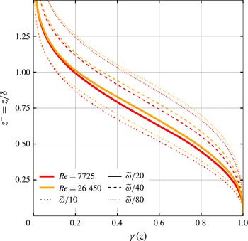
Figure 11. Intermittency factor versus height for the case ri00 and the lower- $Re$
case
$Re$
case $\mathtt{re}\_\mathtt{low}$
with
$\mathtt{re}\_\mathtt{low}$
with $Re=7725$
where the intermittency threshold is varied by a factor of 8 (note that the variation in
$Re=7725$
where the intermittency threshold is varied by a factor of 8 (note that the variation in $Re$
from 7725 to 26 450 corresponds to a variation of
$Re$
from 7725 to 26 450 corresponds to a variation of $\unicode[STIX]{x1D708}$
by a factor of 4).
$\unicode[STIX]{x1D708}$
by a factor of 4).
Appendix A. An inviscid vortex-tilting mechanism in rotating flow
The vorticity equation for Ekman flow reads as
 $$\begin{eqnarray}\displaystyle \frac{\unicode[STIX]{x2202}\unicode[STIX]{x1D74E}}{\unicode[STIX]{x2202}t}+(\boldsymbol{u}\boldsymbol{\cdot }\unicode[STIX]{x1D735})\unicode[STIX]{x1D74E}=(\unicode[STIX]{x1D74E}\boldsymbol{\cdot }\unicode[STIX]{x1D735})\boldsymbol{u}+\unicode[STIX]{x1D708}\unicode[STIX]{x1D6FB}^{2}\boldsymbol{u}+2(\unicode[STIX]{x1D734}\boldsymbol{\cdot }\unicode[STIX]{x1D735})\boldsymbol{u}+2(\boldsymbol{u}\boldsymbol{\cdot }\unicode[STIX]{x1D735})\unicode[STIX]{x1D734}, & & \displaystyle\end{eqnarray}$$
where $\unicode[STIX]{x1D74E}\equiv \unicode[STIX]{x1D735}\times \boldsymbol{u}$
and
$\unicode[STIX]{x1D74E}\equiv \unicode[STIX]{x1D735}\times \boldsymbol{u}$
and $\unicode[STIX]{x1D734}$
is the planetary rotation. It is readily seen that the planetary rotation
$\unicode[STIX]{x1D734}$
is the planetary rotation. It is readily seen that the planetary rotation $\unicode[STIX]{x1D734}$
constitutes a source term in this budget, and rewriting (A 1) in tensor notation, one can use the f-plane approximation to replace
$\unicode[STIX]{x1D734}$
constitutes a source term in this budget, and rewriting (A 1) in tensor notation, one can use the f-plane approximation to replace $2\unicode[STIX]{x1D734}=:2f\hat{e}_{z}$
:
$2\unicode[STIX]{x1D734}=:2f\hat{e}_{z}$
:
 $$\begin{eqnarray}\displaystyle \frac{\unicode[STIX]{x2202}\unicode[STIX]{x1D714}_{i}}{\unicode[STIX]{x2202}t}+u_{j}\frac{\unicode[STIX]{x2202}\unicode[STIX]{x1D714}_{i}}{\unicode[STIX]{x2202}x_{j}}=\unicode[STIX]{x1D714}_{j}\frac{\unicode[STIX]{x2202}u_{i}}{\unicode[STIX]{x2202}x_{j}}+\unicode[STIX]{x1D708}\frac{\unicode[STIX]{x2202}^{2}\unicode[STIX]{x1D714}_{i}}{\unicode[STIX]{x2202}x_{j}^{2}}+f\frac{\unicode[STIX]{x2202}u_{i}}{\unicode[STIX]{x2202}z}. & & \displaystyle\end{eqnarray}$$
Compared with the non-rotating reference frame, there is the additional source $f\unicode[STIX]{x2202}_{z}u_{i}$
representing vortex tilting of planetary vorticity by a vertical gradient of streamwise velocity. This term is also present in the enstrophy equation:
$f\unicode[STIX]{x2202}_{z}u_{i}$
representing vortex tilting of planetary vorticity by a vertical gradient of streamwise velocity. This term is also present in the enstrophy equation:
 $$\begin{eqnarray}\displaystyle \frac{1}{2}\frac{\text{d}\unicode[STIX]{x1D714}_{i}^{2}}{\text{d}t}=\unicode[STIX]{x1D714}_{i}\frac{\unicode[STIX]{x2202}u_{j}\unicode[STIX]{x1D714}_{i}}{\unicode[STIX]{x2202}x_{j}}+\frac{1}{2}\unicode[STIX]{x1D708}\left[\frac{\unicode[STIX]{x2202}^{2}\unicode[STIX]{x1D714}_{i}^{2}}{\unicode[STIX]{x2202}x_{j}^{2}}-2\left(\frac{\unicode[STIX]{x2202}\unicode[STIX]{x1D714}_{i}}{\unicode[STIX]{x2202}x_{j}}\right)^{2}\right]+f\unicode[STIX]{x1D714}_{i}\frac{\unicode[STIX]{x2202}u_{i}}{\unicode[STIX]{x2202}z}. & & \displaystyle\end{eqnarray}$$
In the absence of vorticity, according to (A 2), the sign of $\unicode[STIX]{x1D714}_{i}$
becomes that of
$\unicode[STIX]{x1D714}_{i}$
becomes that of $f\unicode[STIX]{x2202}_{z}u_{i}$
, making the last term of the right-hand side of (A 3) a source of enstrophy. This means that in the presence of even weak velocity gradients in the irrotational region of Ekman flow, vortex stretching of planetary vorticity generates mean vorticity and vorticity at a rate proportional to the velocity gradient
$f\unicode[STIX]{x2202}_{z}u_{i}$
, making the last term of the right-hand side of (A 3) a source of enstrophy. This means that in the presence of even weak velocity gradients in the irrotational region of Ekman flow, vortex stretching of planetary vorticity generates mean vorticity and vorticity at a rate proportional to the velocity gradient $\unicode[STIX]{x2202}_{z}u_{i}$
and the Coriolis parameter
$\unicode[STIX]{x2202}_{z}u_{i}$
and the Coriolis parameter $f$
. At some level of vorticity this process is balanced by dissipation; until this happens vorticity is accumulated in the non-turbulent part of the boundary layer causing a background enstrophy that smears out the jump in enstrophy magnitude between turbulent and non-turbulent parts when compared to other (non-rotating) flows. The
$f$
. At some level of vorticity this process is balanced by dissipation; until this happens vorticity is accumulated in the non-turbulent part of the boundary layer causing a background enstrophy that smears out the jump in enstrophy magnitude between turbulent and non-turbulent parts when compared to other (non-rotating) flows. The $Re$
independence of
$Re$
independence of $\langle u(z)\rangle$
(Ansorge & Mellado (Reference Ansorge and Mellado2014)) in the outer layer suggests that the term
$\langle u(z)\rangle$
(Ansorge & Mellado (Reference Ansorge and Mellado2014)) in the outer layer suggests that the term $f\langle \unicode[STIX]{x1D714}_{x}\rangle \unicode[STIX]{x2202}_{z}\langle u\rangle$
scales inviscidly, and this mechanism is independent of the Reynolds number. The inviscid nature of the vortex-tilting mechanism is seen in figure 11 where the sensitivity of
$f\langle \unicode[STIX]{x1D714}_{x}\rangle \unicode[STIX]{x2202}_{z}\langle u\rangle$
scales inviscidly, and this mechanism is independent of the Reynolds number. The inviscid nature of the vortex-tilting mechanism is seen in figure 11 where the sensitivity of $\unicode[STIX]{x1D6FE}(z)$
to the vorticity threshold does not depend significantly on the Reynolds number. It is concluded that this vortex tilting, irrespective of
$\unicode[STIX]{x1D6FE}(z)$
to the vorticity threshold does not depend significantly on the Reynolds number. It is concluded that this vortex tilting, irrespective of $Re$
, is a fundamental mechanism in Ekman flow rendering the outer, non-turbulent layer different from non-rotating external flows.
$Re$
, is a fundamental mechanism in Ekman flow rendering the outer, non-turbulent layer different from non-rotating external flows.


 Open access