


1. Introduction
The spanwise component of a yawed wind turbine's axial force induces a counter-rotating vortex pair (CVP) that laterally deflects and deforms (Bastankhah & Porté-Agel Reference Bastankhah and Porté-Agel2016; Branlard & Gaunaa Reference Branlard and Gaunaa2016; Howland et al. Reference Howland, Bossuyt, Martínez-Tossas, Meyers and Meneveau2016) its wake downstream. This phenomenon has the potential to increase or regulate wind farm power output (Howland, Lele & Dabiri Reference Howland, Lele and Dabiri2019). Fully harnessing this potential requires a rigorous understanding of the underlying fluid dynamics, as demonstrated by the use of lifting line theory (Shapiro, Gayme & Meneveau Reference Shapiro, Gayme and Meneveau2018) for wind turbine yaw control (Howland et al. Reference Howland, Lele and Dabiri2019). Efficient engineering prediction methods of the mechanisms governing the generation and decay of the induced vorticity downstream of the yawed turbine in the atmospheric boundary layer (ABL) enable wind farm design and operational decisions that take advantage of this knowledge.
The fate of strong streamwise vortices in the ABL, such as the yawed wind turbine CVP, has been studied extensively. Aircraft wings at takeoff generate counter-rotating tip vortices that can stay near the runway and generate dangerous conditions for the next takeoff (Spalart Reference Spalart1998; Gerz, Holzäpfel & Darracq Reference Gerz, Holzäpfel and Darracq2002). From a fundamental fluid dynamics viewpoint, much effort has been invested in understanding the decay process of vortices in turbulent flow (Tombach Reference Tombach1973; Devenport et al. Reference Devenport, Rife, Liapis and Follin1996; Takahashi, Ishii & Miyazaki Reference Takahashi, Ishii and Miyazaki2005; van Jaarsveld et al. Reference van Jaarsveld, Holten, Elesenaar, Trieling and van Heijst2011). In the case of yawed wind turbines, the vast literature on aircraft trailing wake vortices and individual helicoidal vortices shed by individual turbine blades (Ivanell et al. Reference Ivanell, Mikkelsen, Sørensen and Henningson2010; Sørensen Reference Sørensen2011; Chamorro et al. Reference Chamorro, Troolin, Lee, Arndt and Sotiropoulos2013) is useful as a conceptual guide. However, this literature is not directly relevant to the large-scale CVP shed by yawed wind turbines. Their CVP vortex core is expected to scale with the turbine diameter, rather than the chord length of each blade, and their circulation is significantly weaker than that of aircraft trailing vortices since the overall lateral forces generated by the blades sweeping the inclined turbine disk area is only a fraction of the total turbine axial force. Furthermore, the aircraft CVP is initially well approximated by circular vortices, while the yawed wind turbine CVP is initially composed of two vortex sheets.
Recent work is just beginning to link the yawed wind turbine CVP to the aircraft trailing vortex literature: treating the yawed wind turbine as a porous lifting surface and applying Prandtl's lifting line theory, our recent theory predicts the initial magnitudes of the transverse velocity and the circulation of the shed CVP (Shapiro et al. Reference Shapiro, Gayme and Meneveau2018). From this insight, recent work has treated the initial streamwise-vorticity distribution as point vortices (on a plane perpendicular to the flow) along the edge of the swept area of the rotor (Martínez-Tossas et al. Reference Martínez-Tossas, Annoni, Fleming and Churchfield2019; Martínez-Tossas & Branlard Reference Martínez-Tossas and Branlard2020; Zong & Porté-Agel Reference Zong and Porté-Agel2020) that diffuse under turbulent mixing, becoming a distribution of Lamb–Oseen vortices (Saffman Reference Saffman1992). Their lateral diffusion rate is specified by an eddy viscosity that is determined empirically (Zong & Porté-Agel Reference Zong and Porté-Agel2020) or using a mixing length model with the velocity scale specified by the wake velocity gradient and mixing length specified by the size of the largest ABL eddies (Martínez-Tossas et al. Reference Martínez-Tossas, Annoni, Fleming and Churchfield2019). The downstream evolution is then found by numerically integrating the resulting vortex system. This numerical approach yields results that agree well with simulations and experiments, but does not facilitate insight into fundamental vorticity decay mechanisms or reveal scaling laws based on the turbine yaw angle or the ambient turbulence characteristics.
In this work, we study the generation and decay of the CVP generated from yawed wind turbines in the ABL. In order to advance engineering models for the shed vorticity, particularly the total circulation of each vortex, analogous to the Jensen model (Jensen Reference Jensen1983) for the velocity deficit, we seek to derive analytical expressions that do not require numerical integration (Meneveau Reference Meneveau2019). Our model is motivated and validated by large eddy simulation (LES) data, discussed in § 2, and the trailing vortex literature. In § 3, we analytically derive the vorticity, transverse velocity and circulation distribution generated immediately downstream of a yawed actuator disk and compare the analytical predictions to simulations. In § 4, an eddy-viscosity assumption is applied to model the turbulent diffusion during the downstream evolution of this initial vorticity distribution. We propose appropriate velocity and length scales to be used to define an eddy-viscosity that reproduces LES measurements. We derive analytical expressions for the maximum vorticity and total circulation of each vortex and compare these to LES. Of particular interest is to establish whether the decay of the CVP vortex strength can be explained by a simple model of cross-diffusion between the two vortices, an insight that can be used to further refine point vorticity models for wake deformation and curling.
2. Large eddy simulations of yawed wind turbines in the ABL
We study the decay of the vorticity shed from yawed wind turbines in the (neutrally-stratified) ABL using LES of yawed actuator disks. Large eddy simulations are performed with the pseudo-spectral/finite difference code LESGO, which has been used and validated in previous work (Calaf, Meneveau & Meyers Reference Calaf, Meneveau and Meyers2010; Stevens, Martínez & Meneveau Reference Stevens, Martínez and Meneveau2018). The coordinate system  $\boldsymbol {x} = (x,y,z)$ with the unit vectors $\boldsymbol {i}$, $\boldsymbol {j}$, and $\boldsymbol {k}$ is defined such that $x$ is the streamwise direction, $y$ is the spanwise direction, and $z$ is the vertical direction. The origin is placed at the centre of the disk with radius $R = 50$ m. The effective streamwise, spanwise, and vertical domain lengths are $L_x = 3.75$, $L_y = 3$ and $L_z = 1$ km, respectively, and we use $360 \times 288 \times 432$ grid points. Turbulent inflow is generated using a concurrent precursor domain (Stevens et al. Reference Stevens, Martínez and Meneveau2018) with a friction velocity of $u_* = 0.45$ m s $^{-1}$. A shifted periodic boundary condition (Munters, Meneveau & Meyers Reference Munters, Meneveau and Meyers2016) with a $0.49L_z$ shift is used to reduce streamwise streaks in the time-averaged velocity field. The wind turbine with hub height $z_h = 100$ m is placed 500 m downstream of the domain inlet. Subgrid stresses are modelled using the Lagrangian-averaged scale dependent model (Bou-Zeid, Meneveau & Parlange Reference Bou-Zeid, Meneveau and Parlange2005). Wall stresses are modelled using the equilibrium wall model (Moeng Reference Moeng1984) with roughness length $z_0 = 0.1$ m.
The wind turbine is treated as a porous actuator disk that exerts an axial force  $T = -\frac {1}{2} \rho {\rm \pi}R^{2} C_T' u_d^{2}$, perpendicular to the disk, that depends on the local thrust coefficient $C_T'$, disk-averaged velocity $u_d$, disk radius $R$, and the density of air $\rho$. The total axial force $T$ is distributed uniformly across the disk, leading to a distributed force $\boldsymbol {f}(\boldsymbol {x}) = T \mathcal {R}(\boldsymbol {x}) \boldsymbol {n}$, using the normalized indicator function $\mathcal {R}(\boldsymbol {x})$, and points in the unit normal direction to the disk $\boldsymbol {n}$. The yaw angle $\gamma$ is measured counter-clockwise from the positive $x$-axis toward the positive $y$-axis such that the unit normal of the actuator disk is $\boldsymbol {n} = \cos \gamma \boldsymbol {i} + \sin \gamma \boldsymbol {j}$. The normalized indicator function $\mathcal {R}(\boldsymbol{x})=G(\boldsymbol{x}) * \mathcal {I}(\boldsymbol{x})$ is found by filtering (convolving) $\mathcal {I}(\boldsymbol {x}) = {\rm \pi}^{-1} R^{-2}\delta (x) H(R-r)$ (where $\delta (x)$ is the Dirac delta function, $H(x)$ is the Heaviside function and r is the radial distance from the centre of the disk written in terms of the transverse coordinates (i.e. $r^2 = y^2 + z^2$)) with a filtering function $G(\boldsymbol {x})$. The latter is a three-dimensional Gaussian whose width $\sigma _\mathcal {R} = \varDelta / \sqrt {12}$ is equivalent to a top-hat filter (Pope Reference Pope2000) with a filter size chosen as $\varDelta = 1.5h$, where $h = ({\rm \Delta} x^{2} + {\rm \Delta} y^{2} + {\rm \Delta} z^{2})^{1/2}$ is the root mean square of the grid spacings.
Simulations are run for yaw angles of  $\gamma = 15^{\circ }$, $20^{\circ }$, $25^{\circ }$ and $30^{\circ }$ with a local thrust coefficient of $C_T' = 1.33$. Velocity fields are time-averaged for a time ${\mathcal {T}}$ where ${\mathcal {T}} u_*/L_z \approx 8$ (all variables in this paper are time-averaged). A representative time-averaged streamwise vorticity $\omega _x$ field for
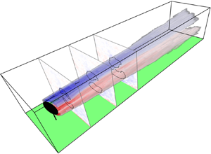
  $\gamma = 20^{\circ }$ is shown in figure 1. The vorticity contour plots and volume rendering show the initial generation of arcs of vorticity above and below the turbine line of symmetry. These arcs decay downstream, each tending to a more axisymmetric distribution. The bottom vortex becomes flattened, presumably due to the action of the ground. Furthermore, secondary vortex structures are generated at the ground.

Figure 1. Time-averaged streamwise vorticity distribution behind a yawed wind turbine with  $\gamma = 20^{\circ }$ under turbulent ABL inflow. (a) Volume rendering of the vortex core with (b–d) contour plots of the total streamwise vorticity. Vortex cores are outlined in black.
Even with the significant time-averaging and shifted periodic boundary conditions of the inflow, some background (noisy) vorticity is evident in the contour plots. To distinguish between the shed CVP and the background vorticity, we apply Otsu's method (Otsu Reference Otsu1979) on the positive and negative vorticity at each cross-plane. Otsu's method maximizes the intercategory (or minimizes the intracategory) variance, and thus identifies the region with the strongest coherent vorticity, which we define as the vortex core.
To determine the circulation of each vortex as a function of  $x$, we numerically integrate the vorticity over the core area to obtain $\varGamma _{core}(x)$. The core vorticity ratio $\alpha (x) = \omega _{Otsu}(x)/\omega _{max}(x)$ is defined as the ratio of the thresholding value on vorticity that separates the core vortex region from the remaining vorticity $\omega _{Otsu}(x)$ to the maximum vorticity magnitude $\omega _{max}(x)$. The total circulation of each vortex is then estimated as $\varGamma (x) =\varGamma _{core}(x)/(1-\alpha (x))$. This approach exactly recovers the total circulation of a Lamb–Oseen vortex (Saffman Reference Saffman1992). The downstream evolution of maximum vorticity magnitudes $\omega _{max}(x)$ and circulations $\varGamma (x)$ for each $\gamma$ measured from LES and normalized by the inlet velocity $U_\infty$ and disk diameter $D=2R$ are shown in figure 2. We see similar decaying behaviour for all yaw angles with the bottom vortex initially having a greater core circulation than the top vortex and decaying more quickly. Unlike the peak vorticity that begins to decay immediately downstream of the turbine, the circulation stays nearly constant up to $x/D\sim 3$ and only then begins its decay downstream.

Figure 2. (a) Maximum vorticity magnitude and (b) circulation magnitude for top (blue and negative) and bottom (red and positive) vortices with  $\gamma = 15^{\circ }$ ( $\raisebox{3pt}_{\Box}}$), $20^{\circ }$ ( $\circ$), $25^{\circ }$ ( $\diamond$) and $30^{\circ }$ ( $\vartriangle$).
A number of vortex decay mechanisms have been discussed (van Jaarsveld et al. Reference van Jaarsveld, Holten, Elesenaar, Trieling and van Heijst2011), such as viscous diffusion, strong external turbulence, cross-diffusion across the line of symmetry, and Crow instability breakup. When turbulence levels and shed vorticity strength are moderate, evidence from many of these earlier simulations points to the cross-diffusion mechanism (Cantwell & Rott Reference Cantwell and Rott1988; Ohring & Lugt Reference Ohring and Lugt1993; van Dommelen & Shankar Reference van Dommelen and Shankar1995; Leweke, Dizès & Williamson Reference Leweke, Dizès and Williamson2016) playing a dominant role. In the following sections, we develop a model first to predict the generation and then the decay of the yawed wind turbine CVP.
3. Generation of counter-rotating vortices from yawed actuator disks
We first model the generation of the vorticity at the rotor plane. By approximating the elliptic projection of the transverse force of an actuator disk as a circle, the transverse force can be written as
 \begin{equation} f_y = -{\tfrac{1}{2}}\rho C_T U_\infty^{2} \cos^{2} \gamma \sin \gamma H(R-r) \delta (x), \end{equation}
where  $C_T$ is the standard thrust coefficient, $r$ is the radial distance along the disk and $\theta$ is the polar angle measured from the positive $y$-axis toward the positive $z$-axis, i.e. $\sin \theta = z/r$. Taking the curl of the mean momentum equation, linearizing the advective term, and neglecting turbulent and viscous stresses, the linearized mean streamwise vorticity transport equation (also used in Martínez-Tossas, Churchfield & Meneveau Reference Martínez-Tossas, Churchfield and Meneveau2017) becomes
 \begin{equation} U_\infty \partial_x \omega_x= - \rho^{-1} \partial_z\,f_y. \end{equation}
Writing the derivative of the transverse force in terms of the cylindrical coordinate system using the chain rule, using (3.1) and integrating (3.2) yields the vorticity distribution
 \begin{equation} \omega_x(x,r,\theta) = -{\tfrac{1}{2}} C_T U_\infty \cos^{2}\gamma \sin \gamma \sin \theta \delta(r-R) H(x). \end{equation}
Integration of the vorticity (3.3) just downstream of the disk over the top and bottom half-planes yields the circulation of both the top and bottom shed vortices
 \begin{equation} \varGamma_{top} = -\varGamma_{bottom} = \int_0^{\infty} \int_{0}^{\rm \pi} \omega_x(0^{+},r,\theta) r \, \textrm{d}\theta \, \textrm{d} r = -R C_T U_\infty \cos^{2} \gamma \sin \gamma. \end{equation}
The vortices are counter-rotating with a circulation magnitude  $\varGamma _0 = R C_T U_\infty \cos ^{2} \gamma \sin \gamma$, which is identical to the predictions from lifting line theory (Shapiro et al. Reference Shapiro, Gayme and Meneveau2018).
The vorticity predicted by (3.3), which is valid for an idealized actuator disk, is now compared to numerical simulations of a yawed actuator disk under uniform inflow from Shapiro et al. (Reference Shapiro, Gayme and Meneveau2018). In numerical simulations using a filtered force, the effective radius of the wind turbine is  $R_* = R + 0.75h$ (Shapiro et al. Reference Shapiro, Gayme and Meneveau2018), where $h = ({\rm \Delta} x^{2} + {\rm \Delta} y^{2} + {\rm \Delta} z^{2})^{1/2}$ is the grid size. When comparing analytical predictions to numerical simulations, we use this effective radius and circulation $\varGamma _0^{*} = R_* C_T U_\infty \cos ^{2} \gamma \sin \gamma$. The vorticity distribution can be approximated by first mapping (3.3) with an effective radius $R_*$ and circulation $\varGamma _0^{*}$ onto an arc-shaped line, where $\omega _x(\chi ,\zeta ) =- [\varGamma ^{*}_0/(2R_*)] \sin (\chi /R_*) \delta (\zeta )$, $\chi = \theta r$, and $\zeta = r-R_*$. This vorticity is then filtered (convolved) with a two-dimensional Gaussian $G_2 = (2{\rm \pi} \sigma _\mathcal {R}^{2})^{-1}\exp (-(\chi ^{2}+\zeta ^{2})/2\sigma _R^{2})$ whose width $\sigma _\mathcal {R}$ is equal to the filtering kernel used to filter the axial force to obtain
 \begin{equation} \omega_x(\theta,r) = -\frac{\varGamma^{*}_0}{2R_*} \frac{\sin (\theta r/R_*)}{\sigma_\mathcal{R} \sqrt{2 {\rm \pi}}} \exp\left( - \frac{(r-R_*)^{2}}{2 \sigma_\mathcal{R}^{2}} \right) \exp\left( - \frac{\sigma_\mathcal{R}^{2}}{2R_*^{2}} \right). \end{equation}
As can be seen in figure 3 for the case with  $C_T' = 0.8$ and $\gamma = 20^{\circ }$, the vorticity distribution predicted by (3.5), figure 3(a), reproduces the numerical results, figure 3(d), with the simulation performed for the same parameters. For comparison to simulations, the thrust coefficient is calculated based on the local one used for the simulations according to $C_T = 16 C_T'/(4+C_T'\cos ^{2}\gamma )^{2}$ (Shapiro et al. Reference Shapiro, Gayme and Meneveau2018).

Figure 3. Near rotor (a,d) streamwise vorticity, (b,e) spanwise velocity and (c,f) vertical velocity distributions from a yawed actuator disk with  $C_T' = 0.8$ and $\gamma = 20^{\circ }$, with laminar inflow. Top panels show values measured at $x=R$ and bottom panels show theory. A circle with radius $R_*$ is shown in black in all panels.
To validate the vorticity generation model, we also compare induced velocities by applying the Biot–Savart law in the near turbine region:
 \begin{equation} v(\boldsymbol{x}) = -\frac{1}{4{\rm \pi}} \int \frac{\omega_x(\boldsymbol{x}') (z - z')}{\vert \boldsymbol{x} - \boldsymbol{x}'\vert^{3}} d^{3} \boldsymbol{x}', \quad w(\boldsymbol{x}) = \frac{1}{4{\rm \pi}} \int \frac{\omega_x(\boldsymbol{x}') (y - y')}{\vert \boldsymbol{x} - \boldsymbol{x}'\vert^{3}} d^{3} \boldsymbol{x}'. \end{equation}
Integrating in the radial direction we obtain
 \begin{equation} v(\boldsymbol{x}) = \frac{1}{8{\rm \pi}} \frac{\varGamma_0}{R} \int_{0}^{\infty} \int_{0}^{2 {\rm \pi}} \frac{ R \sin \theta' (r \sin \theta - R\sin \theta') \, \textrm{d}\theta' \, \textrm{d}\kern0.8pt x'}{\left[(x-x')^{2} + (r\cos \theta - R \cos \theta')^{2} + (r\sin \theta - R \sin \theta')^{2}\right]^{{3}/{2}}}, \end{equation}
and integration in the streamwise direction (Gradshteyn & Ryzhik Reference Gradshteyn and Ryzhik1980, #2.271.5) yields
 \begin{equation} v(\boldsymbol{x}) = \frac{1}{8{\rm \pi}} \frac{\varGamma_0}{R} \int_{0}^{2 {\rm \pi}} R \sin \theta' (r \sin \theta - R\sin \theta') \left[ \frac{1}{a} + \frac{1}{a} \frac{x}{(a + x^{2})^{1/2}} \right] \textrm{d}\theta', \end{equation}
where  $a = (r\cos \theta - R \cos \theta ')^{2} + (r\sin \theta - R \sin \theta ')^{2}$. We are primarily interested in $v$ at $x >>R$ or $x>>a$, leading to $v=-\varGamma _0/4R$ and $w=0$ for $r \le R$, and $v = -[{\varGamma _0}/({4R})] (R/r)^{2}\cos (2\theta )$ and $w = -[{\varGamma _0}/({4R})] (R/r)^{2}\sin (2\theta )$ for $r > R$. The $w$ component has been found by using the continuity equation. Inside the radius of the actuator disk, the $v$ velocity component ( $\varGamma _0/4R$) is identical to the constant prediction from lifting line theory (Shapiro et al. Reference Shapiro, Gayme and Meneveau2018), and the $w$ component vanishes. Outside the radius of the actuator disk, the velocity components depend on the polar angle and decrease with the squared radial distance.
The predictions for  $v$ and $w$ are compared to simulations for $C_T' = 0.8$ and $\gamma = 20^{\circ }$ measured at $x = R$ in figure 3(b,c,e,f). To compare the theoretically predicted velocity components to simulation results, the velocity must be sampled before the self-induction of the vorticity is considerable. However, directly downstream of the actuator disk, the actuator disk streamtube is still expanding from the non-negligible streamwise pressure gradient induced by the streamwise component of the axial force. To counteract this effect in the simulation measurements, we have removed the expansion expected from a decelerating streamtube by plotting $v + u_r\cos \theta$ and $w + u_r \sin \theta$, where $u_r$ is the radial velocity. The radial velocity is obtained by measuring the streamwise velocity gradient at the centre of the actuator disk streamtube (assuming that $\partial _x u= \partial _x u(R,0,0)$ for $r \le R^{*}$ and $\partial _x u = 0$ for $r > R^{*}$) and radially integrating the continuity equation, i.e. $u_r = ({r}/{2}) \partial _x u(R,0,0)$ for $r \le R^{*}$ and $u_r = ({R_*^{2}}/{2r}) \partial _x u(R,0,0)$ for $r > R_*$. With this correction included, the velocity components agree well with simulations, thus further supporting the predicted generated vorticity distribution described in (3.3).
4. Turbulent decay of counter-rotating vortices in the ABL
We now consider the decay of the CVP due to the surrounding turbulence in the ABL and test the implications of the cross-diffusion hypothesis (Cantwell & Rott Reference Cantwell and Rott1988; Ohring & Lugt Reference Ohring and Lugt1993; van Dommelen & Shankar Reference van Dommelen and Shankar1995). In our simplified model, the self-induced deformation of the shed vorticity sheet is neglected, the ABL shear is also neglected, and only turbulent diffusion is considered. The boundary-layer assumptions are applied to the streamwise vorticity equation downstream of the turbine (Saffman Reference Saffman1992; Pope Reference Pope2000), and (3.2) is replaced by an advection–diffusion equation with eddy viscosity  $\nu _T(x)$:
 \begin{equation} U_\infty \partial_x \omega_x = \nu_T(x) \left(\partial_y^{2} \omega_x + \partial_z^{2} \omega_x \right). \end{equation}
 First, note that a point vortex  $\omega _x(x_0,y,z) = \varGamma _p \delta (y-y_0) \delta (z-z_0)$ with circulation $\varGamma _p$ located at $(x_0,y_0,z_0)$ that evolves under (4.1) diffuses downstream (Saffman Reference Saffman1992) as
 \begin{equation} \omega_x(x,y,z) = \frac{\varGamma_p}{4 {\rm \pi}\eta^{2}(x)}\exp\left(-\frac{(y-y_0)^{2} + (z-z_0)^{2}}{4 \eta^{2}(x)}\right), \end{equation}
where the length scale  $\eta (x)$ results from the integral of the eddy viscosity
 \begin{equation} \eta^{2}(x) = U_\infty^{-1} \int_{x_0}^{x} \nu_T(x') \, \textrm{d}\kern0.8pt x'. \end{equation}
The virtual origin  $x_0$ is introduced to account for the finite thickness of the initial vorticity distribution, which depends on the grid size in simulations or potentially the chord size of a physical turbine. The solution in (4.2) is equivalent to filtering the initial condition with a two-dimensional Gaussian kernel with a width of $\sqrt {2}\eta (x)$, since the underlying governing equation (4.1) is linear. This result is then applied to the initial vorticity distribution (3.3) generated by the yawed turbine by placing point vortices around the circle with radius $R$ at locations $(x_0,R\cos \theta , R\sin \theta )$ with differential circulation $\textrm {d}\varGamma _p = -\varGamma _0\sin \theta /2 \, \textrm {d}\theta$. Integrating around the circle leads to the vorticity field
 \begin{equation} \omega_x(x,y,z) = -\int_0^{2{\rm \pi}} \frac{\varGamma_0 \sin\theta}{8 {\rm \pi}\eta^{2}(x)} \exp\left(-\frac{(y-R\cos\theta)^{2} + (z-R\sin\theta)^{2}}{4 \eta^{2}(x)}\right) \textrm{d}\theta. \end{equation}
While (4.4) cannot be integrated directly for all  $y$ and $z$, the integral of (4.4) coincident with the peak vorticity magnitude at $y=0$ and $z = \pm R$ can be integrated as
 \begin{equation} \omega_{max}(x) = \frac{\varGamma_0}{R^{2}} \frac{R^{2}}{4 \eta^{2}(x)} \exp\left( - \frac{R^{2}}{2\eta^{2}(x)}\right) I_1\left( \frac{R^{2}}{2\eta^{2}(x)}\right), \end{equation}
where  $I_n$ is the modified Bessel function of the first kind with order $n$.
$n$.
The total circulation in the vortex system generated by a yawed actuator disk vanishes in all streamwise planes, i.e.  $\varGamma _{total}(x) = \int _{-\infty }^{\infty } \int _{-\infty }^{\infty } \omega _x(x,y,z) \, \textrm {d} y \, \textrm {d} z = 0$, because the vorticity across the $y$-axis is equal and opposite. Here, we have neglected the image vorticity due to the ground interaction. Integrating each vortex $\varGamma (x) = \vert \int _{0}^{\infty } \int _{-\infty }^{\infty } \omega _x(x,y,z) \, \textrm {d} y \, \textrm {d} z \vert = \vert \int _{-\infty }^{0} \int _{-\infty }^{\infty } \omega _x(x,y,z) \, \textrm {d} y \, \textrm {d} z \vert$ yields a normalized circulation
 \begin{equation} \frac{ \varGamma(x) }{\varGamma_0}= \frac{\sqrt{\rm \pi}}{4}\frac{R}{\eta(x)} \exp\left( - \frac{R^{2}}{8\eta^{2}(x)}\right)\left[ I_0\left( \frac{R^{2}}{8\eta^{2}(x)}\right) + I_1\left( \frac{R^{2}}{8\eta^{2}(x)}\right)\right], \end{equation}
whose magnitude monotonically decreases for  $\eta \ge 0$. This decrease in circulation is caused purely by the cancellation of vorticity along the $y$-axis as vorticity diffuses downstream.
The problem of properly specifying the eddy viscosity is approached using a mixing length model  $\nu _T(x) = \upsilon \ell$, where $\upsilon$ is a velocity scale and $\ell$ is the mixing length (Pope Reference Pope2000). The appropriate velocity and length scales are specified using reasoning analogous to that described in Shapiro et al. (Reference Shapiro, Starke, Meneveau and Gayme2019) for wind turbine wakes. For a free wake, the mixing length scales with the wake width and the scale of the velocity fluctuations are proportional to the velocity deficit (Pope Reference Pope2000). In the ABL, however, turbulent mixing of the wake is dominated by the boundary-layer induced turbulence, whose fluctuations are proportional to the friction velocity. Therefore, the appropriate velocity scale is the friction velocity, i.e. $\upsilon \sim u_*$, and the appropriate length scale is the wake size (Shapiro et al. Reference Shapiro, Starke, Meneveau and Gayme2019). For a vortex in the ABL, the reasoning remains the same and the eddy viscosity is $\nu _T = u_* \ell$, where $\ell$ is the size of the vortex.
In order to specify the size of the vortex, we turn to similarity scaling for wakes in the ABL (Shapiro et al. Reference Shapiro, Starke, Meneveau and Gayme2019), where the wake grows linearly with downstream distance, i.e.  $\ell \sim x$. Equivalently, the Jensen wake model (Jensen Reference Jensen1983) assumes that the diameter of a top-hat wake is $D_w = D + 2kx$, where $k$ is the wake expansion rate commonly taken as $k = u_*/U_\infty$. Applying the log law to the inlet velocity $U_\infty = (u_*/\kappa ) \ln (z_h/z_0)$, where $\kappa =0.4$ is the von Kármán constant, results in an expansion rate that depends on the hub height and roughness height $k = \kappa /\ln (z_h/z_0)$. We assume that the vorticity grows at the same rate $2kx$, but initially starts with thickness much smaller than $D$. In order to write $\ell$ in terms of the Jensen model top-hat length scale, we note that a point vortex filtered with a box filter with a scale $\beta$ has the same second moment (Pope Reference Pope2000) as a diffused point vortex with length scale $\beta /\sqrt {24}$. Therefore, we write the mixing length as $\ell = 2 k (x-x_0)/\sqrt {24}$. Thus the resulting eddy viscosity and squared length scale are, respectively, modelled according to
 \begin{equation} \nu_T(x) = u_* 2k(x-x_0)/\sqrt{24} \quad\mbox{and, from (4.3),}\ \eta^{2}(x) = k^{2} (x-x_0)^{2} /\sqrt{24}. \end{equation}
 The maximum vorticity, circulation and vortex growth rate are compared to data from simulations in figure 4. In the model, the virtual origin  $x_0$ is chosen by noting the equivalence between the effect of diffusion with a length scale $\eta$ to Gaussian filtering with a length scale $\sqrt {2}\eta$. Considering the filtered axial force with length scale $\sigma _\mathcal {R} = \varDelta /\sqrt {12}$, we conclude that the virtual origin is $x_0 = -24^{-1/4}\varDelta /k$. A similar effect is expected for either a physical wind turbine or a drag disk, where the thickness of the initial vorticity distribution will scale with the chord of the blades or thickness of the disk. In figure 4, we compare the model predictions with the arithmetic average of LES measured peak vorticity and circulation magnitudes from the top and bottom vortices, since the simulation data showed some differences between the top and bottom vortices and these differences are not captured by the current theory. Results shown in figure 4(c,d) also indicate that the normalizations by $R_*$ and $\varGamma _0^{*}$ suggested by the theory for maximum streamwise vorticity (4.5) and circulation (4.6) (with effective parameters in LES $R_*$ and $\varGamma _0^{*}$ determined as explained in § 3) yield good collapse of the LES data and with the theory.

Figure 4. Maximum vorticity and circulation magnitude normalized by (a,b) rotor diameter  $D$ and inlet velocity $U_\infty$ and (c,d) theoretical circulation $\varGamma _0^{*}$ and effective radius $R_*$. (e; inset to a) Vortex radius showing linear growth. Symbols show simulation results (the arithmetic average of the magnitudes corresponding to top and bottom vortices) and lines show theory, i.e. (4.5) for panels (a,c), (4.6) for panels (b,d) and (4.8) for panel (e), the inset in panel (a).
In order to validate the growth rate of the mixing length, we calculate the vortex radius from simulations, which is defined as the location of the maximum spanwise velocity above the rotor  $r_1(x) +R = {argmax}\, v(x,0,z)$. For a Lamb–Oseen vortex, which is expected beyond $x/D > 5$, the vortex radius is (Saffman Reference Saffman1992)
 \begin{equation} r_1 = 2.24 \eta = 2.24 (24)^{-({1}/{4})} k(x-x_0) \approx k(x-x_0),\quad \text{with}\ k=u_*/U_\infty. \end{equation}
As shown in the inset to figure 4(a), the growth rate of the measured vortex radius is linear with  $x$ and agrees with the theory.
Consideration of the transformation of the vorticity from a diffused line around the edge of the disk to a diffused point vortex as well as the length scale  $\eta (x)$ reveals power-law scalings for the maximum vorticity. Initially, the vorticity is confined to a line around the edge of the disk. Considering this limiting case with $z$ being the coordinate normal to the line, $U_\infty \partial_x \omega _{x} = \nu_T(x) \partial _z^{2} \omega _x$ with $\omega _x(\boldsymbol x, 0) = \varGamma _p \delta (z)$, yields the solution $\omega _x = [\varGamma _p/(\eta (x) \sqrt {4{\rm \pi} })] \exp (-z^{2}/(4\eta ^{2}(x))$, with maximum circulation scaling inversely with the length scale $\omega _{max} \sim \eta ^{-1}$. In the far field, the vorticity behaves like a point vortex, as derived earlier, with the expected scaling of $\omega _{max}(x) \sim \eta ^{-2}$. With the virtual origin from the simulations $x_0 \approx -2D$, the squared length scales as $\eta ^{2}(x) \sim x^{2}+4xD+4D^{2}$. Therefore, for moderate $x/D \approx 2$, where the $4xD$ term is the same order as the $4D^{2}$ term and dominates the $x^{2}$ term, the squared length scale initially scales as $\eta ^{2}(x) \sim x$. For large $x/D$, the squared length scales as $\eta ^{2}(x) \sim x^{2}$. Combined with the scaling of line and point vortices, this yields the following power laws for the maximum vorticity: $\omega _{max} \sim x^{-1/2}$ for moderate $x/D$ and $\omega _{max} \sim x^{-2}$ for large $x/D$. These scaling laws agree well with simulations and theory, as shown in figure 4(c).
5. Discussion and conclusions
Using concepts drawn from the aircraft trailing vortex literature (Cantwell & Rott Reference Cantwell and Rott1988; Ohring & Lugt Reference Ohring and Lugt1993; van Dommelen & Shankar Reference van Dommelen and Shankar1995; Spalart Reference Spalart1998), we study the decay of the vortices generated by yawing of wind turbines. The theory presented in §§ 3 and 4 considers the effect of linear advection and turbulent diffusion on the decay of the vorticity and circulation shed from yawed turbines. The analysis is based on a streamwise-varying eddy viscosity that depends on the growth rate of the vorticity length scale and the boundary-layer friction velocity. The analysis enables us to obtain analytical expressions for the maximum vorticity and shed circulation from each counter-rotating vortex that agrees well with actuator disk simulations of yawed wind turbines in the ABL. Results refine the emerging understanding of the decay of the vorticity shed from yawed turbines. As in Shapiro et al. (Reference Shapiro, Starke, Meneveau and Gayme2019), we find that careful consideration of the appropriate mixing length and velocity scale for the eddy viscosity of wind turbines in the ABL yields an eddy viscosity that increases linearly with downstream distance and a mixing length that grows at a rate  $k=u_*/U_\infty$. While thermal stability is not directly considered in the model so far, the effects of thermal stratification could be incorporated using, e.g. Monin–Obukhov similarity theory to introduce a stability correction factor in estimating the vortex expansion rate $k$.
$k$.
The results provide a theoretical framework for engineering models of the shed vorticity consisting of closed-form analytical expressions, i.e. (4.5), (4.6) and (4.8). These do not require numerical integration of differential equations to evaluate the model, hence facilitating eventual use in engineering models for wind farm design and control. The expressions for total circulation of the vortices is particularly useful for models that consider the yawed turbine CVP as a pair of Lamb–Oseen vortices. The scaling also agrees well with the empirical observation of Zong & Porté-Agel (Reference Zong and Porté-Agel2020) in the near field of the wake.
Turbulent mixing appears to be the dominant process that governs the decay of the shed vorticity. The yawed turbine generates equal and opposite circulation bound to the rotor disk that is shed downstream, resulting in vanishing total circulation. For a single vortex, the circulation would remain constant even as the vorticity diffuses downstream. However, since the opposing negative vorticity similarly diffuses, the cancellation of the diffused vorticity along the centreline of the wake results in the apparent ‘dissipation’ of circulation for the entire system. The cross-diffusion hypothesis, however, does not fully explain the apparent differences between the top and bottom vortices in the CVP. Ground effects, vertical shear and the vertical structure of turbulence in the ABL clearly play a role in creating some differences in the evolution of the top and bottom vortices that more refined models should also aim to reproduce.
Acknowledgements
The authors acknowledge funding from the National Science Foundation (grant nos 1949778 and 1635430) and computational resources from MARCC and Cheyenne (doi: 10.5065/D6RX99HX).
Declaration of interests
The authors report no conflict of interest.


