II. GORDON’S PATHWAY IN ECONOMICS AND FISHERY SCIENCE

Howard Scott Gordon was born in 1924 in Halifax, Nova Scotia. He graduated from Dalhousie University in 1944, then won a scholarship to study for his master’s degree at Columbia University, New York. Gordon then went back to Canada for a fellowship at McGill University, Montreal, in 1947–48, where he started teaching economics. In 1948, Gordon was appointed assistant professor at the newly created university of Carleton, Ottawa, where he helped set up the Department of Economics. He was head of the department until he left for Indiana University in 1966.

To consider Gordon as a resource economist, in the sense that he would have spent his entire career in the field, would be an exaggeration, notwithstanding the fact that the field of environmental and natural resource economics, as we know it, had not yet been established in the 1940s and 1950s (Pearce Reference Pearce2002; Kula Reference Kula2006; Banzhaf Reference Banzhaf2019, Reference Banzhaf2023; Berta, Debref, and Vivien Reference Berta, Debref and Vivien2021). In fact, fisheries were only one of his many interests. He started with research in macroeconomics and economic policies (see, for instance, his master’s thesis, entitled “The Concept and Components of National Savings in the Canadian Economy,” Gordon Reference Gordon1947) and then moved to the history of economic thought (Fox and Gordon Reference Fox and Gordon1951) and the philosophy of economics and epistemology (Gordon Reference Gordon1950). His doctoral dissertation, defended in 1953, focused on the role of theory in economic thought through an overview of the epistemology of John Maynard Keynes, Karl Marx, and Alfred Marshall (Gordon Reference Gordon1953a). His contribution to resource and fishery economics consists of seven publications, dating between 1951 and 1958. After 1958, he apparently stopped working on natural resources, to come back to macroeconomics and the philosophy of economics. At Indiana University, he focused on the history of social sciences. Margaret Schabas, who had studied under Gordon, praised him for being one of the first historians of economic thought to “break away” from economics departments to join a department of history and philosophy of science (Schabas Reference Schabas1992, p. 192f).

Gordon started working on fisheries in 1948, after his arrival in Ottawa, where he met Fred Popper from the government’s Fisheries Department economics office, who would later join the United Nations’ Food and Agriculture Organization (Scott Reference Scott2011, p. 78). He then “began to do occasional work for the Canadian Department of Fisheries” (Gordon Reference Gordon1984, p. 14). In the summer of 1951, Gordon was employed by the department’s Fisheries Price Support Board to carry out a field study on behalf of the Prince Edward Island Fisheries Development Committee. This work, which Gordon (Reference Gordon1984, p. 14) himself years later described as “extremely practical and empirical,” aimed to survey the possibilities for development of the fishing industry and led to a report, published one year later, entitled “The Fishing Industry of Prince Edward Island” (Gordon Reference Gordon1952b). The scope of the report was not limited to the catching activity per se but covered the whole fishing industry, from the “primary industry—the catching” (Gordon Reference Gordon1952b, p. 1) to “processing, transportation and marketing” (p. 35). In the first section, devoted to the catching industry, Gordon gave a detailed account of the economic situation of Prince Edward Island’s different fisheries by compiling statistics on landings for several species and their market prices, the number of fishermen involved in the fishery, their equipment, and their revenue. In this report, Gordon mainly built on field observations and descriptive statistics, tabulated or plotted on graphs. His main conclusion was that several of the island’s fisheries, particularly for lobster, were exploited inefficiently from an economic point of view. Landings had not risen in years, whereas the number of traps and fishermen had increased substantially. Hence, he pointed out the waste due to the inadequate use of man-made factors of production, which resulted in low wages for the too numerous fishermen involved.

From that empirical work, Gordon began to move towards theorization. In 1953, he published a first theoretical article in the Journal of the Fisheries Research Board of Canada, entitled “An Economic Approach to the Optimum Utilization of Fishery Resources.” In this first version of his economic analysis of fisheries, Gordon drew on graphical analysis to explain fishermen’s lack of profit. Assuming a decreasing marginal product from fishing with respect to the effort employed and a constant marginal cost of effort, he showed that the optimum, defined as the maximization of net product received by fishermen, would be achieved by equalizing marginal cost and marginal revenue. However, Gordon identified the lack of property rights over the resource as an obstacle to achieving this optimization. Because an additional fisherman would consider only the “average production” he would obtain by joining the fishery before deciding whether or not to do so, fishermen would enter the race for fish until marginal cost equaled average (rather than marginal) production, hence dissipating the rent that could have been obtained (Gordon Reference Gordon1953b).

Gordon therefore developed theoretical tools in the tradition of marginal analysis, in the vein of Frank Knight and Arthur Cecil Pigou,Footnote ⁴ to look for a fundamental root to what he had witnessed in the field: a growing number of poor fishermen fighting over a limited number of potential catches. In this context, the “overexploitation” of a marine resource, defined in economic terms as inefficient exploitation, was due to a property issue and the result of competition for “common-property” resources: “The argument of the following few pages is that the overexploitation of fishing grounds which is so widely encountered is due to powerful economic forces. The fundamental cause of this overexploitation is the fact that fishing grounds are, in most cases, the common property of all who may wish to use them” (Gordon Reference Gordon1953b, pp. 449–450; emphasis in the original).

Gordon would follow this road towards theorization and generalization with his 1954 article. After the publication in a subject-specific and non-economic periodical in 1953, Gordon attempted to publish in economic journals. He succeeded with a publication in the Journal of Political Economy in April 1954.Footnote ⁵ The title of his article, “The Economic Theory of a Common-Property Resource: The Fishery,” shows an additional step towards generalization: the fishery had become only an illustration for a more general problem in natural resource economics. The core of the article is essentially a reworking of the 1953 paper, with the presentation, in section 3, “The Economic Theory of the Fishery,” of the graphical analysis of the rent dissipation mechanism in fisheries due to the common-property issue. However, at the end of this section, Gordon added an extensive discussion about the specificity of halieutic resources compared, for example, with agricultural resources, and presented several examples of similar configurations of non-appropriability for other resources—for instance, “common pasture” and petroleum. This development was a means of advocating the generality of his argument about common-property resources and the necessity of implementing property rights in these cases (Gordon Reference Gordon1954, pp. 134–135).

The other major difference between the two articles is the addition, in the fourth and last section of the 1954 paper (entitled “The Bionomic Equilibrium of the Fishing Industry”), of a heuristic algebraic model to support his theoretical analysis. Gordon described the “bionomic ecosystem” (Reference Gordon1954, p. 141) of a theoretical fishery with five variables: P, E, L, C, and R representing respectively the fish population, the fishing effort (or intensity), the total catch, the total cost of fishing, and the revenue of fishermen. They were linked by four equations, and a fifth one gave a first order condition of revenue maximization (with a, b, c, and q being parameters, respectively the maximum population of the fish species, a “depletion coefficient,” a “technical coefficient of production,” and the cost per unit of fishing effort; Gordon Reference Gordon1954, pp. 141–142):

(1) $$ P=a- bL $$

(2) $$ L= cEP $$

(3) $$ C= qE $$

(4) $$ R=L-C $$

(5) $$ \frac{dR}{dE}=0 $$

These equations made it possible to prove, not only graphically but analytically, the existence of different equilibria and a maximum for fishermen’s profit. With the help of his colleague Malcolm C. Urquhart (Gordon Reference Gordon1954, p. 124f), this model was conceived after the publication of the first article, during the summer of 1953, when Gordon participated in the first Summer Study Group at Queen’s University (Rymes Reference Rymes1991, p. 2). This attempt at formalization in a mathematical model can be viewed as another step by Gordon in the direction of theory and abstraction, contributing to the extension of mathematization in the discipline of environmental and natural resource economics.

However, the status of the model in Gordon’s work is more ambiguous than it seems. The vision of his article as a purely heuristic theoretical contribution to economics has to be challenged: the model might be viewed also as a predictive practical tool, designed to help in defining actual management policy for fisheries. Fishery biologists started to use algebraic models to describe the effect of fishing on fish stocks in the 1930s and used them in actual management programs to determine the type and magnitude of regulation needed. Tim D. Smith (Reference Smith1994) shows how fishery science has developed as an applied science, with constant to-ing and fro-ing between empiricism and theorization. Algebraic models representing the dynamics of exploited fish populations were developed in various fisheries management institutions, in parallel with population ecology modeling, with few interactions between these research programs. Fishery biologists concentrated on the impact of exploitation on fish populations, and built models that they intended to be simple and practical for management, often by focusing on one mechanism that they identified as the main determinant of dynamics: individual growth, recruitment, fishing mortality, etc. We can cite, for instance, William F. Thompson, who modeled the effect of fishing on age class structures at the Pacific Halibut Commission (T. D. Smith Reference Smith1994, p. 212); William E. Ricker, and his “spawner and recruit theory” developed to help regulate the sockeye salmon fishery on the Fraser River, British Columbia (T. D. Smith Reference Smith1994, p. 287); and the research program conducted by Oscar E. Sette, John C. Marr, and Milner B. Schaefer for the California sardine fishery that eventually led to Schaefer’s “surplus production theory” that allows for the determination of the Maximum Sustainable Yield (MSY), which was then “adopted as a goal of management” in “many international fisheries agreements made during the 1950s” (T. D. Smith Reference Smith1994, p. 264). Gordon’s attempts to formalize his analysis in a simple algebraic model were in line with this specific tradition of fishery science modeling.

Moreover, in the second section of his 1954 article, Gordon discussed several general claims on the influence of fishing activity on fish populations (among others, Ricker’s and Thompson’s) and criticized biologists’ earlier work in fishery science for not considering the economic aspects of the matter, in particular the cost of fishing. This shows Gordon’s willingness to participate in debates within fishery science about fisheries management, aside from his efforts to theorize about a broader category of economic resources. If we follow Morgan and Morrison’s (Reference Morgan and Morrison1999) framework, Gordon sought to ensure that his model would have both a heuristic theoretical exploration function and a “mediating” function between economic theory and fisheries management for public policy design. Gordon’s interest in practical management issues can also be traced back to his empirical study for the development of the Prince Edward Island fisheries industry, and can be identified as well in his 1953 article, where he dedicated the last section to “practical management policy” (Gordon Reference Gordon1953b, pp. 454–457).

Gordon had the ambition of rendering his 1954 model applicable to real-life fisheries, thanks to further statistical research that would allow the parameters to be determined—i.e., by calibrating the model. From this perspective, Gordon published another article in the Journal of the Fisheries Research Board of Canada one year later, based on an econometric study of Fisheries Department catch data. Gordon drew an explicit link between this study and his algebraic model in the introduction to this 1955 article. He conceded that the 1954 model was not yet practical, because it required “estimates of the absolute size of the species population under natural conditions and a ‘depletion coefficient’ that measures the reduction in the population brought about by different catch levels” (Gordon Reference Gordon1955, p. 85). Although the article did not provide estimates for such parameters, and studied only macro-level statistical correlations between national economic indicators and total catches of different species, it was presented by Gordon as a first step in the direction of more predictive empirical studies that would lead to the “determination of the optimum level of exploitation” (p. 85). In a letter he sent to Edgar H. Hollis, fishery scientist at the U.S. Fish and Wildlife Service, Gordon formulated this ambition even more clearly:

Gordon’s ambition was, therefore, twofold: on the one hand, to contribute to natural resource economics theory by providing a heuristic theoretical analysis of an abstract resource category, and, on the other hand, to actually participate in building effective predictive tools to be used in fisheries management, thus competing with fishery biologists. The bioeconomic model was at the crossroads of these two ambitions. However, it is easy to imagine how these two goals might have come into conflict in the process of model building. The degree of abstraction, the need to be empirically grounded, and even the choice of decision variables can differ widely between a heuristic economic model and a more applied, predictive, policy-oriented one. The next section explores how this tension was translated into the construction of the production function.

III. FROM AN ECONOMIC ANALYSIS OF FISHERIES TO A BIOECONOMIC FUNCTION OF PRODUCTION

Gordon was able to label his model “bioeconomic” thanks to the consideration, in the system of equations, of the fish population, via the variable P. However, a closer look at Gordon’s previous work shows that this focus on fish populations was not something he had developed from his earlier papers but rather represented a departure from his previous method of analyzing fisheries. It is thus useful to reconstruct Gordon’s path towards the formal analysis of production in fisheries, from his early empirical work in 1952, to understand how he came to this modeling choice and how far his model could be considered integrated.

When looking at the development of the Prince Edward Island fishing industry, Gordon already had in mind the need for an economic representation of fisheries production processes. In his 1952 report, he distinguished three factors of production: fishermen, their gear and equipment, and the “natural resources they attempt to exploit” (Gordon Reference Gordon1952b, p. 15). There was a clear asymmetry in the analysis of these factors, however: although human factors were precisely identified and measured, Gordon remained vague about the importance of natural factors. He placed them outside the scope of his analysis because they were “primarily biological in nature” and hence would be better analyzed by biologists (p. 27). The only way Gordon alluded to their importance in the production process was when they were identified as limiting production, for instance in the lobster fishery, where catches were stagnating, in spite of the increase in the quantity of other human factors of production employed (pp. 22–23, 30).

Starting with his 1953 article, Gordon formalized his work on fisheries production via a mathematical function whose properties were central for his reasoning and the demonstrations he made. Particularly interesting for us is the evolution of the justification of these properties, between 1953 and 1954, that brings to light an ambiguity in the biological foundations of the model.

In his 1953 article, Gordon assimilated the function that associated landings with fishing intensity (the “landings function,” p. 444) to a production function for fisheries. It was a function of one variable, the effort of fishing, that thus played the role of a factor of production. Interestingly enough, Gordon gave no definition of the effort. It was actually a concept that had been widely used for years in fishery science at the time Gordon wrote, being used to represent the intensity of fishing (see, for instance, Ricker Reference Ricker1940, Reference Ricker1944; Schaefer Reference Schaefer1943). In economic terms, it translated an aggregate of human factors of production, that is to say, labor and capital: in other words, the fishermen and their gear that Gordon studied statistically in 1952. Although the two factors were aggregated into one variable, the production function presented in 1953 embodied a rather standard vision of production, from capital and labor, and without an explicit representation of natural resources as a factor of production.

He then discussed the properties of this function with graphical illustrations. Specifically, he claimed that the function should have the same shape as “a standard ‘production function’ of economic theory” and hence be subject to diminishing returns (at least after a certain point) (Gordon Reference Gordon1953b, p. 444). All the graphs in his article then represented landings functions that increased with a diminishing slope, i.e., concave functions. This property of the function was actually crucial for his demonstration, since the formal determination of the equilibrium rests upon the shapes of landings and cost curves. Gordon therefore spent a large portion of his article on the justification of the concavity of the function. In doing so, he insisted on making a clear distinction between two possible justifications to this property: on the one hand, the reduction in the total number of fish, which would make each additional effort less successful in catching fish; and, on the other hand, what he refers to as the “law of diminishing returns” (pp. 444–446).

A brief article written by Gordon (Reference Gordon1952a), and published one year earlier under the title “On a Misinterpretation of the Law of Diminishing Returns in Marshall’s Principles,” helps to make this distinction clearer. In this article Gordon pointed out what seemed to him an inconsistency in Marshall’s work. According to Gordon, Marshall took a slightly different definition of the law when he illustrated it with respect to fisheries than he had with other examples. Marshall previously defined it as the decrease in productivity when increasing only one factor, ceteris paribus. It is the proportion of factors that changes as the first one is increased. However, when discussing fisheries, Marshall pointed out that, as the labor factor increased, another factor—the number of fish in the sea—decreased, leading to a decrease in fishing productivity. The ceteris paribus condition was not respected here, and the same law was expressed as a result of a change in quantities of factors.Footnote ⁷

Gordon thus drew a clear analytical distinction between the law of diminishing returns and the retroaction of fishing on the productivity of fishing effort via the reduction of the fish stock. And in his 1953 article, although he let the door open to different explanations, Gordon chose to consider only the first as an explanation of the concavity of the production function. Gordon assumed that the population was fixed, and that diminishing returns were due to the law, that is to say the varying proportions of factors when more fishing effort was applied. The provenance of the diminishing returns is thus not perfectly clear, since he did not give any indication of the precise mechanisms that resulted in this decrease in productivity of effort. The only justification in the article is a short reductio ad absurdum, eventually dropped in the 1954 article, that the law of diminishing returns must apply in some way, otherwise an infinite quantity of fish could be caught in a fixed area.

In the 1954 article, Gordon insisted again on the necessity of a “nonlinear” (actually concave) function of production, so that the model can be analytically solved, since “stable equilibrium requires that either the cost or the landings function be nonlinear,” and he saw no obvious reason to consider costs that were not linear in efforts (Gordon Reference Gordon1954, p. 137). Although this idea of concavity as a necessity for analysis was already present in the 1953 article, a major difference may be noted between the two papers. In 1954, Gordon claimed that the basis for this nonlinearity was the “population effect,” that is to say the reduction of the fish population by fishing, and no longer the law of diminishing returns. Although he still insisted on making a clear analytical distinction between the two, this time he supposed that the law of diminishing returns, understood in terms of proportion of factors, did not apply to fisheries. Instead he “[assumed] that, as fishing effort expands, the catch of fish increases at a diminishing rate but that it does so because of the effect of catch upon the fish population” (p. 129).

The “population effect” was embodied in the algebraic model that was also added to the 1954 article, with the introduction of the population variable P and an expression for it. The first equation of the system reflects the fact that the equilibrium population is diminished by fishing. The second expresses landings as a function of both effort and population:

(6) $$ P=a- bL $$

(7) $$ L= cEP $$

The production (landings) function had now become a function of two variables, representing biological and economic factors of production. And it was the combination of this function with the first equation that gave the expression of the production as depending only on fishing effort:

(8) $$ L=\frac{caE}{1+ cbE} $$

This function is indeed concave: the formal property of the function had been turned into a consequence of a hypothesis that comes from fishery science (the fact that fishing negatively impacts the equilibrium fish population), rather than an assumption, which comes from a general economic law for production. Our inquiry therefore allows us to identify a reversal of Gordon’s justification of a formal property of his model that is central to his demonstration, between 1953 and 1954. Although the concavity of the function is deduced from assumptions (both biological and economic) in the 1954 algebraic model, we were able to show that the concavity preceded, in time, its final justification. Our history of the construction of the model shows that the fish population variable and the property that comes with it (the population effect) arrived in extremis in Gordon’s analysis, when he finally decided to formalize it with an algebraic model.

This observation opens up the question of Gordon’s methodology, in terms of integrated model building. More specifically, the consideration of the fish population is what enables the model to be considered as bioeconomic, i.e., bringing together biological and economic variables. This cross-cutting dimension can be said to be substantial, since a biological variable, with a property apparently coming from fishery science (population is diminished by fishing), is at the core of the model, with the production function’s property deriving from it. However, our reconstruction of the model-building process puts the idea of an integrated approach into perspective. The methodology employed by Gordon to deal with halieutic resources did not seem originally to build on any specific characteristic of the resource. He applied a generic production model, as if the fishing industry was analogous to any other industry. Gordon’s postulate on the form of the production relied on a generic economic law of diminishing returns that originated in agricultural production analysis and was then applied to various industries. Gordon’s methodology in his early work thus seems to be primarily targeted towards providing a compact, synthetic, heuristic model for theoretical exploration, where the concrete specificity of halieutic resources is set aside to make room for a standard economic analysis of production. His position would thus be closer to a tendency to reductionism or methodological bias among economists when analyzing natural resources that have their own complexity and that are not a priori economic objects (Pottier Reference Pottier2014; Missemer Reference Missemer2017; Couix Reference Couix2019). Although he did, eventually, substitute a formal biological foundation for an economic one in his bioeconomic model, Gordon did not explicitly comment on the inclusion of the fish population as a core element of the model. He recognized the “population effect” as being better than a more formal and abstract justification for the concavity of the production function, but we cannot exclude the possibility that the introduction of a population equation was a kind of ad hoc biological justification that hid Gordon’s prioritizing of heuristics over predictive realism. Possibly, he saw this change as a way to legitimize his work in the field of fishery biology, without having to reconsider his model. It can hence be viewed as opportunistic and weaken the hypothesis that Gordon’s work contains a substantial integrated modeling methodology. However, as we will see, the introduction of a population variable would prove to be decisive for the later connection between biologists’ research and Gordon’s.

IV. GORDON AND SCHAEFER: STATIC ECONOMICS AND BIOLOGICAL DYNAMICS

Although Gordon’s model was built partly to compete with biologists in defining fisheries management policy, its biological foundations do not appear as clearly as often claimed via the presence of a function for population dynamics. As we have seen, the model did contain an equation for the fish population, similar in this respect to the fishery scientists’ model, but, in contrast, theirs were typically dynamic. The bioeconomic model of 1954 is in fact static, since none of the five equations, already presented above, are time-dependent. Gordon built on this static system for his demonstration with the hypothesis that cost is a linear function of effort; landings and profit were expressed as functions of one variable, the effort of fishing; and the model was analytically solved to determine the optimal effort. Gordon hence introduced no dynamics for the fish population in his model—in particular, he did not rely on Schaefer’s equation, contrary to what is often argued (for instance, by Munro Reference Munro1992, p. 165; T. D. Smith Reference Smith1994, p. 335; Quinn Reference Quinn2008, p. 359; White Reference White2008, p. 423). He took into consideration the population only from a static viewpoint, via its equilibrium value. Gordon considered that the population can be in equilibrium at any level between 0 and a, with fishing acting only to withdraw fish, moving the population away from its maximum, as shown by equations (1)-(5).

One reason why Gordon did not integrate Schaefer’s research on population dynamics into his model is that Gordon was, as far as we know, unaware of Schaefer’s work in 1953–54. A first draft of Schaefer’s “surplus production theory” was introduced in a research report by Schaefer, Oscar Sette, and John Marr (Reference Schaefer, Sette and Marr1951), as part of their project on the California sardine fishery, but it might not have been widely disseminated outside fishery biologist communities, and Gordon made no reference to it in his work. The theory was formally introduced by Schaefer in an article published in the Bulletin of the Inter-American Tropical Tuna Commission in 1954. A letter sent by Gordon to Schaefer a few months after the publication of his own 1954 article suggests that he had not read this article before, since he asked for a copy of it, specifying that it was recommended by Ricker, who was a mutual acquaintance.Footnote ⁸

In contrast, Schaefer had read Gordon’s 1953 article in June 1954, as indicated by the compliments addressed in the letter Schaefer sent in response to Gordon’s,Footnote ⁹ and read the Journal of Political Economy article in around May 1955.Footnote ¹⁰ Schaefer recognized the potential of Gordon’s model but also identified room for improvement and intended to pursue Gordon’s attempt by making his own contribution to fishery economics. He sent a draft to Gordon, asking for feedback in around May 1956, and, after some exchanges that did not lead to substantial changes to the core of the article, Schaefer had it published in January 1957 in the Journal of the Fisheries Research Board of Canada (where Gordon published his Reference Gordon1953b and Reference Gordon1955 fisheries articles).Footnote ¹¹ Schaefer explicitly framed it as a response to Gordon’s modeling attempt. He pointed out the fact that Gordon did not take into account the biological specificity of the halieutic resources, not only their renewability but their “autoregulatory” character, by not explicitly representing fish population dynamics in his mathematical model (Schaefer Reference Schaefer1957, p. 670). More precisely, Schaefer criticized Gordon’s decision to focus on an equilibrium population and the way he modeled it, by a linearly decreasing function of landings (p. 674). Schaefer therefore proposed an algebraic model that addressed the limitations he identified, by integrating into Gordon’s model an explicit dynamics for the fish population. The dynamic model selected by Schaefer was based on previous research that identified the logistic curve as an adequate model for population change (Schaefer, Sette, and Marr Reference Schaefer, Sette and Marr1951; Schaefer Reference Schaefer1954b, Reference Schaefer1954a). This model was founded on the hypothesis that the population growth rate depends only on the size of the population itself, following a dome-shaped curve. It demonstrated a form of autoregulation within the population: the growth rate is null for a population of zero individuals, maximal for a certain number of fish, and null again when the number of fish reaches a maximum (set by the carrying capacity of the environment). Schaefer translated it algebraically using a quadratic form (Schaefer Reference Schaefer1957, p. 673):

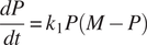(9) $$ \frac{dP}{dt}={k}_1P\left(M-P\right) $$

with M the maximum population and k₁ a constant. He then added the fishing effect as a withdrawal of fish that hinders the growth of the population:

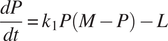(10) $$ \frac{dP}{dt}={k}_1P\left(M-P\right)-L $$

Schaefer, looking for potential equilibrium of exploitation, focused on situations where the growth of the population was null, to obtain a simple equation linking population and catches:

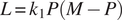(11) $$ L={k}_1P\left(M-P\right) $$

This equilibrium equation is analogous to equations (1)-(5) in Gordon’s model and can take its place in the system of equations to form a bioeconomic model based on a biological dynamics. That is what Schaefer did in the rest of the 1957 article, which allowed him to analyze the different possible equilibria of the fishery (depending on what management objective is chosen) known today as Maximum Sustainable Yield (MSY), Maximum Economic Yield (MEY), and Open-Access equilibrium (OA).Footnote ¹²

The story of the coupling between biology and economics in the Gordon–Schaefer model must thus be told in the opposite manner to that in which it is often presented. It was not Gordon in 1954 but Schaefer three years later who integrated biological dynamics into the economic model. He started from Gordon’s modeling work and added the final touch to the bioeconomic model we know today under the name of Gordon–Schaefer.

Since Gordon did not base his model on Schaefer’s logistic growth equation, it may seem unexpected that Schaefer was so easily able to plug his dynamic equation into the static economic model. As Schaefer stated in his article, they disagreed on one of the basic assumptions of their models: the relationship between fish population and landings. Gordon assumed that a fixed population was given every year and that fishing acted as a withdrawal of fish, while Schaefer considered changes in population size as a dynamic process, depending both on the present size of the population and on the fishing pressure. These conceptions led them to different representations of the landings-effort curve: ever-increasing but at a diminishing rate for Gordon and dome-shaped for Schaefer. Thus, a question of compatibility arises between two separately created economic and biological models. What was the common denominator between them that allowed such an easy connection?

To understand how this was possible, it is useful to turn first to a round table on fishery economics organized by the Food and Agriculture Organization of the United Nations in 1956, which Gordon joined, and the proceedings of which were published one year later (Turvey and Wiseman Reference Turvey and Wiseman1957). In particular, the paper presented by the Canadian economist Anthony D. Scott helps to shed light on the link between Gordon and Schaefer. Scott was familiar with Gordon’s work, since he published an article that built on the 1954 model a year later (Scott Reference Scott1955), but was also aware of Schaefer’s ongoing work. He had read Schaefer’s draft, thanks to Gordon, and corresponded with Schaefer about this work before the conference. At the round table, Scott presented a new version of his 1955 model, where he substituted Schaefer’s relationship between effort and landings for Gordon’s, built around the idea that the specificity of halieutic resource was its capacity to renew itself at a natural rate that could vary according to biological and environmental factors (including fishing). Scott had been convinced by his exchanges with Schaefer that the latter’s model more accurately reflected the biological dynamics, but he also realized how easy it was to make the substitution.Footnote ¹³ During the conference, Scott detailed his vision of the common ground between Gordon and Schaefer’s models by underlining the crucial implication of Schaefer’s biological model: the fish population could be kept in equilibrium at any size, provided that the catch rate equaled the growth rate. According to Scott, this idea, described as “equilibrium catch” by Schaefer (Reference Schaefer1954b), was common to both Gordon’s and Schaefer’s work, allowing compatibility between their models: “This is my understanding of the idea of ‘equilibrium catch’ implicit in Professor Gordon’s paper, loc. cit., p. 137, and expounded in greater detail in ‘Some Aspects of the Dynamics of Population Important to the Management of the Commercial Marine Fisheries’, by Milner B. Schaefer” (Scott Reference Scott, Turvey and Wiseman1957, p. 48n).

The concept can, indeed, be identified in Gordon’s article, when he described the effect of fishing on population as simply moving a pre-existing ecological equilibrium downwards: “If a species were in ecological equilibrium before the commencement of commercial fishing, man’s intrusion would have the same effect as any other predator; and that can only mean that the species population would reach a new equilibrium at a lower level of abundance” (Gordon Reference Gordon1954, p. 128; emphasis added).

In Gordon’s model, this idea was translated by the first equation of the bioeconomic system. The modeling of the equilibrium population linearly decreasing with catches embodied the idea of equilibrium catch, as clearly stated in the page of Gordon’s article that Scott refers to in his presentation: “a postulated catch … connotes an equilibrium population in the biological ecosystem” (Gordon Reference Gordon1954, p. 137).

Schaefer’s equation that links landings and population fits Gordon’s model because they both rely on the same hypothesis of the existence of an equilibrium possible for every level of fishing. But if this idea is for Schaefer a corollary of a biological theory of population dynamics, it appears as a hypothesis in Gordon’s work and there is no apparent justification for it: as Scott (Reference Scott, Turvey and Wiseman1957, p. 48n) pointed out, the idea of equilibrium catch is only implicit in Gordon’s model. Gordon did not explicitly refer to any biological theory that would justify the possibility of equilibrium catches at any level of population, although he cited many fishery biologists in his article. He seemed to take this idea of equilibrium as self-evident. Although this hypothesis in Gordon’s work seems to question the biological foundations of his model, our inquiry allowed us to track back a possible biological inspiration that would legitimize Gordon’s assumption: in the work of the English biologist Edward S. Russell.

Russell was a pioneer of fishery science in the 1930s. He is best known for having been one of the first to propose a formal algebraic breakdown of changes in fish stocks, hence establishing the framework for various pieces of modeling work that occurred in fishery science over the following decades. In Smith’s words he “[provided] a clear and simple framework for using a priori methods” (T. D. Smith Reference Smith1994, p. 202). In the second section of his 1954 article, Gordon cited Russell’s seminal article (Russell Reference Russell1931), as well as a collection of lectures entitled The Overfishing Problem (Russell Reference Russell1942) in the same footnote, as an illustration of the “‘modern formulation’ of the fisheries problem” (Gordon Reference Gordon1954, p. 128). Although this reference does not provide direct evidence of an important link between Russell’s theory and Gordon’s model, a letter sent by Gordon in 1956 to Clyde C. Taylor, biologist and assistant chief of the North Atlantic Fishery Investigations in the Fish and Wildlife Service of the United States Department of the Interior, enables us to identify quite a strong connection. In this letter, Gordon answered a critique that he received from Taylor regarding the shortcomings of the biological side of his model. In his response, the only reference to a biologist’s work that he puts forward is Russell’s The Overfishing Problem, which he claims to have read before writing his article.Footnote ¹⁴

Reading Russell’s book is indeed enlightening, for it allows us to understand where Gordon is likely to have found a biological assumption that legitimizes the focus on equilibrium population and the use of a static method to model his bioeconomic system. In the fourth lecture of the 1942 book, Russell discussed changes in a theoretical fish population when affected by different factors (fishing, natural mortality, individual growth, and recruitment). This lecture includes reflections that are very close to the equilibrium catch idea as seen in Gordon’s article. More specifically, Russell claimed that the population can be in equilibrium at any level, depending mainly on the intensity of fishing: “It is obvious that a stock can be stabilised at different levels of density, and that the level will depend mainly upon the rate of capture, since this is the factor that mainly determines the age-distribution of the stock, through fishing mortality” (Russell Reference Russell1942, p. 83). He developed this idea by describing the mechanisms behind the stabilization of the population that occurs when the intensity of fishing changes: “Actually, with any given capture rate, provided it is sufficiently great to be an important factor in mortality, we may expect rate of growth and average rate of recruitment to adjust themselves to it, and the same will hold good of the rate of natural mortality” (Russell Reference Russell1942, p. 84).

The idea of equilibrium catch as understood by Gordon’s model can thus be traced back to the work of the biologist Russell. Moreover, there is a clear filiation between the theoretical framework established by Russell and Schaefer’s modeling work. Indeed, as Tim D. Smith (Reference Smith1994, p. 324) shows, Schaefer’s model is an attempt to build upon Russell’s idea by formalizing, with a growth function, the adaptation of the growth rate to the capture rate that allows an equilibrium to be maintained. The compatibility between Gordon’s and Schaefer’s model, explained by the reliance on a common concept of equilibrium catch, can therefore be linked to the inspiration they both found in Russell’s work. The identification of a likely biological inspiration for Gordon’s bioeconomic model is an important result, since it was not explicit in Gordon’s article, and left open the question of its ex post compatibility with Schaefer’s biological work. More precisely, the fact that Gordon took the fish population as a variable in his model and included an equation for the action of fishing upon the population constituted an obvious first step toward formal compatibility with the biologists’ model. But a more substantial compatibility was needed to allow for a simple substitution of Gordon’s population equation for another one: that is exactly what Russell’s theory provided.

V. HEURISTICS VS. PREDICTION: GORDON’S FINAL TAKE ON FISHERY ECONOMICS

When we consider again Gordon’s model-building methodology, our inquiry into the inspiration behind his consideration of population leads to an original conclusion. Gordon did not take a ready-to-use, already formalized theory of the effect of fishing upon fish populations and plug the equation in his model—in fact, he created his own equation. Hence, Gordon’s modeling work cannot be described as an operation of simply coupling biological and economic equations, since he most likely made up his own equation to represent a biological assumption.

In retrospect, this methodology is all the more intriguing given that there were ready-to-use theories available for Gordon to build a coupled bioeconomic model at the time. Indeed, it seems that Gordon was aware of contemporary literature in fishery biology when he conceived his article. Many of the authors he cited in his article had by that time proposed formalized theories for the dynamics of exploited populations that could have formed the basis of a mathematized economic model. Russell’s first general algebraic formulation of the breakdown of population change was already more than twenty years old (Russell Reference Russell1931), and other fishery scientists that Gordon read, such as Ricker and Thompson, but also Raymond J. H. Beverton and Michael Graham, had built more detailed formalized models on this basis. These models shared the general assumptions of fishery sciences (a focus on the fish population rather than the individual fish, a utilitarian vision of the fish as a potential catch) and a mathematical formalism that made them compatible with economic modeling. Considering the state of the art in fishery biology at the time and the proliferation of theories that built on Russell’s framework, we must explain Gordon’s choice of mathematically translating a concept based on previous work in fishery biology. We turn to two complementary explanations that can help us to understand this aspect of Gordon’s model-building methodology.

First, if Gordon did search for the best population equation, the complexity of mathematical dynamics equations might have acted as a deterrent to his ambition of providing a compact model for economic theorization. At the time, population models taken from fishery biology could be mathematically sophisticated and not easily translated into readable and tractable forms: Beverton’s work, for instance, relied on complex integral calculus. Gordon’s aim when building his heuristic economic model might have pushed him to search for the most compact expression. In Gordon’s previously quoted letter to Taylor, in response to the biologist’s invitation to consider some modeling work he did, inspired by Beverton, Gordon explicitly stated his confusion regarding the complexity of population dynamics models—including Russell’s simpler equation—and his intention to rely on “simplifying concepts”:

Notwithstanding the mathematical complexity of the biological theories of the time, it is unlikely that Gordon actually reviewed them in order to integrate the most appropriate one into the model. As we have seen previously, the focus on fish populations arrived late in Gordon’s work and was not considered from the beginning as a central point for the analysis, i.e., Gordon’s 1954 model was not integrated. What mattered for the demonstration of the dissipation of the rent was the shape of the production function. When he changed the justification to account for the “population effect,” he probably sought the mathematical expression that would embody this mechanism in the clearest way, a linearly decreasing function, without seeking the most realistic function in the fishery science literature. The idea of equilibrium catch, probably found in Russell’s work, was the “simplifying concept” that was sufficient for Gordon to legitimize the form he built for the population equation. This method—translating one of the core assumptions into the purest mathematical form—matched his heuristic goal with the model. It was effective, in the sense that Gordon’s model could be used to identify the lack of property rights as the source of rent dissipation and hence poverty among the too numerous fishermen—which he initially observed in the field. In that respect, Gordon’s work mirrored what other economists were doing at that time, e.g., Robert M. Solow and Paul A. Samuelson’s work in macroeconomics, where compacity and simplicity were viewed as a virtue of models (Boumans Reference Boumans and Morgan2001; Cherrier Reference Cherrier2023).

In the end, it seems that, in the tension between the two ambitions of Gordon’s model, the balance eventually tipped in favor of heuristic economic theorization rather than predictive public-policy fisheries management, based on up-to-date fishery biology. As Marcel Boumans and Mary S. Morgan (Reference Boumans and Morgan2001) have noted, in modeling as in material experiments, there is a trade-off between the control that can be exercised over the model or experiment and the possibility of inference about the world via its manipulation. In that regard, simplifying assumptions like Gordon’s render the model more flexible as a heuristic device and thus fruitful for constructing theories but at the same time can limit its applicability. Gordon had certainly thought about the next step that would render his model applicable, by calibrating it with additional econometric work. However, he did not pursue this line of research, and one may wonder whether the calibration could have been possible with Gordon’s assumption about fish population dynamics at the core of the model. Gordon’s ambition for a future calibration of his compact model reminds us of what Boumans (Reference Boumans2001, p. 449) says about later modeling tradition: “economists, after a century of mathematical modeling, now prefer very simple mechanisms with the faith that they will be calibrated in the future.”

Nonetheless, Schaefer’s a posteriori biological foundations eventually reopened the door for the predictive, applied aim of the model. It is interesting in that regard to notice that Gordon finally approved the substitution of the logistic model for his population equation: although he did not seem convinced by Schaefer’s curve when they first corresponded,Footnote ¹⁶ at the round table in Rome, when Scott presented the coupling of his model with Schaefer’s, Gordon said that the “curve (rate of growth of population of a fish stock of a given species) was much closer to the latest biological theory than were earlier ones” (Turvey and Wiseman Reference Turvey and Wiseman1957, p. 59). Maybe this recognition was related to the fact that Schaefer’s curve allowed the model to become more realistic, and more likely to become a tool for actual management of fisheries, but without losing its compactness, maneuverability, and hence its heuristic properties. Containing both of its qualities, the integrated model, under the name of Gordon–Schaefer, could then be the basis of both theoretical work in economics (notably in fishery economics, but more generally in natural resource economics, with the dynamic model of natural resources exploitation by Vernon L. Smith [Reference Smith1968], for instance) and applied work for fisheries management, with complexification on both the biological and the economic side, thanks notably to the work of Colin W. Clark (Reference Clark1976) and his handbook Mathematical Bioeconomics.