


1. Introduction
It is well-known that suspensions of sinking or motile particles can form patterns spontaneously due to instabilities in the uniform base state. For example, in a dilute suspension of identical sinking prolate spheroids or rods, the seminal paper by Koch & Shaqfeh (Reference Koch and Shaqfeh1989) demonstrated the instability that gives rise to the streamer structure. The mechanism is as follows. A perturbation in the spatial distribution of the negatively buoyant particles creates a shear flow that attracts more particles towards regions of higher particle concentration, thereby creating a positive-feedback self-focusing mechanism and resulting in the streamer structures. Under the assumption of a Stokes flow, Koch & Shaqfeh (Reference Koch and Shaqfeh1989) showed that the zero wavenumbers are the most unstable, implying that there would be only a single streamer spanning the width of the container, but the experiments of Metzger, Butler & Guazzelli (Reference Metzger, Butler and Guazzelli2007a,Reference Metzger, Butler and Guazzellib) have shown otherwise. Later, Dahlkild's linear analysis (Reference Dahlkild2011) showed that a finite Stokes number could regularise wavenumber, and Zhang, Dahlkild & Lundell (Reference Zhang, Dahlkild and Lundell2013) further extended the analysis nonlinearly and studied the effect of hydrodynamic diffusion. There were also other attempts to explain the discrepancy (e.g. Saintillan, Shaqfeh & Darve Reference Saintillan, Shaqfeh and Darve2006), but the wavelength selection of streamers remained an open question (Guazzelli & Hinch Reference Guazzelli and Hinch2011).
In the meantime, monodisperse motile particle suspensions were also analysed in a similar way. Pedley, Hill & Kessler (Reference Pedley, Hill and Kessler1988) first demonstrated how gyrotaxis of bottom-heavy motile particles could destabilise a uniform suspension into bioconvective patterns. Gyrotaxis describes the tendency for bottom-heavy motile particles to swim sideways under shear due to the competing torque from the local vorticity and gravity. Although not recognised at the time, the mechanism of the gyrotactic instability is physically the same as the aforementioned instability and results in a similar plume structure. Like Dahlkild (Reference Dahlkild2011), Pedley et al. (Reference Pedley, Hill and Kessler1988) included the effect of finite unsteadiness due to fluid inertia. However, the finite wavelength corresponding to the most unstable mode remained larger than the experimental observation. Instead, Pedley et al. (Reference Pedley, Hill and Kessler1988) highlighted that the steady bioconvective patterns have a wavelength smaller than the initial disturbance. This phenomenon was also observed in the experiments of sinking rods (Metzger, Guazzelli & Butler Reference Metzger, Guazzelli and Butler2005; Metzger et al. Reference Metzger, Butler and Guazzelli2007b).
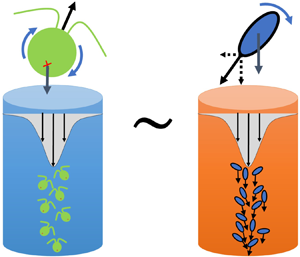
Despite the apparent similarity, gyrotactic plumes and streamers in settling spheroids/rods were treated historically as two separate topics. This work will report an interesting analogy between the two phenomena by comparing them under the same framework, treating the buoyant and orientable particles as a continuum phase under the dilute assumption. We will show that the gyrotactic plumes and streamers are not only physically similar but mathematically equivalent, driven by the same nonlinear particle-flow coupling that is analogous to another well-studied phenomenon known as chemotactic collapse. This comparative study will provide a unifying framework to compare the three phenomena, enabling an exchange of knowledge between the topics and bringing new light to open questions on the wavelength selection of streamer structures.
2. Formulation
2.1. The Fokker–Planck (Smoluchowski) equations
It has been well-established that the trajectory  $\dot {\boldsymbol {x}}^*$ of an orientable particle (‘particle’ hereafter) suspended in the presence of ambient flow $\boldsymbol {u}^*$ can be written as
 \begin{equation} \dot{\boldsymbol{x}}^* = \boldsymbol{u}^* + \boldsymbol{v}_s^*(\,\boldsymbol{p}), \end{equation}
where  $\boldsymbol {v}_s^*(\,\boldsymbol{p})$ is the slip velocity of the particle that depends on its orientation. In this work, we will consider two kinds of particles: sinking prolate spheroids (as an approximation for rods), and spherical gyrotactic swimmers (as a model for gyrotactic motile micro-organisms such as the bottom-heavy micro-algae Chlamydomonas). For a sinking spheroid with density $\rho ^* + {\rm \Delta} \rho ^*$, equatorial radius $a^*$ and polar length $AR a^*$ suspended in a fluid of density $\rho ^*$ and viscosity $\mu ^*$, the slip velocity can be written as
 \begin{equation} \boldsymbol{v}_s^*(\,\boldsymbol{p}) = v_\bot^* \boldsymbol{e}_g+(v_\parallel^*-v_\bot^*) (\boldsymbol{e}_g\boldsymbol{\cdot}\boldsymbol{p})\boldsymbol{p}. \end{equation}
Here,
 \begin{equation} v_\parallel^* = \frac{2}{9}\,\frac{{\rm \Delta}\rho^*\,g^* (a^*)^2\,AR}{\mu^*}\,X (AR) \quad \mbox{and} \quad v_\bot^* = \frac{2}{9}\,\frac{{\rm \Delta}\rho^*\,g^* (a^*)^2\,AR}{ \mu^*}\,Y (AR) \end{equation}
are the sinking speeds when the particle's orientation  $\boldsymbol {p}$, defined by the axis of revolution of the spheroid, is parallel and perpendicular to gravity $g^* \boldsymbol {e}_g$. Here, both $X (AR)$ and $Y (AR)$ are functions of the aspect ratio $AR$, the detailed formula of which can be found in Appendix A (cf. Kim & Karrila Reference Kim and Karrila1991). Meanwhile, for a spherical gyrotactic swimmer, the slip velocity is
 \begin{equation} \boldsymbol{v}_s^*(\,\boldsymbol{p}) = v_\bot^* \boldsymbol{e}_g+v_c^* \boldsymbol{p}. \end{equation}
In this work, the superscript  $*$ indicates dimensional variables or parameters.
Since the velocity  $\dot {\boldsymbol {x}}^*$ depends on the orientation $\boldsymbol {p}$, the particle's angular velocity must also be resolved simultaneously. For a spheroid, the angular velocity is governed by the Jeffery orbit (Bretherton Reference Bretherton1962)
 \begin{equation}
\dot{\boldsymbol{p}}
^*=\tfrac{1}{2}\boldsymbol{\varOmega}^*\times\boldsymbol{p}+
\alpha_0\boldsymbol{p}\boldsymbol{\cdot}\boldsymbol{\mathsf{E}}^*\boldsymbol{\cdot}
(\boldsymbol{I}-\boldsymbol{p}\boldsymbol{p}),
\end{equation}
\begin{equation}
\dot{\boldsymbol{p}}
^*=\tfrac{1}{2}\boldsymbol{\varOmega}^*\times\boldsymbol{p}+
\alpha_0\boldsymbol{p}\boldsymbol{\cdot}\boldsymbol{\mathsf{E}}^*\boldsymbol{\cdot}
(\boldsymbol{I}-\boldsymbol{p}\boldsymbol{p}),
\end{equation}
where  $\boldsymbol{\mathsf{E}}^*= \frac {1}{2} (\boldsymbol {\nabla }^* \boldsymbol {u}^* + (\boldsymbol {\nabla }^* \boldsymbol {u}^*)^{\rm T})$, and $\boldsymbol {\varOmega }^* = \boldsymbol {\nabla }^* \times \boldsymbol {u}^*$ are the local rate-of-strain and vorticity, and $\alpha _0=(AR^2-1)/(AR^2+1)$ is the Bretherton constant. Meanwhile, the orientational trajectory of a spherical gyrotactic particle is
 \begin{equation} \dot{\boldsymbol{p}} ^*= \frac{1}{2 B^*}[-\boldsymbol{e}_g + (\boldsymbol{e}_g \boldsymbol{\cdot} \boldsymbol{p})\boldsymbol{p} ] +\frac{1}{2}\,\boldsymbol{\varOmega}^*\times\boldsymbol{p}, \end{equation}
where  $B^*$ is the gyrotactic time scale. The orientation $\boldsymbol {p}$ can also be written in terms of the Euler angles $\theta,\phi$ relative to the spatial coordinates $\boldsymbol {x}=(x,y,z)^{\rm T}$ as shown in figure 1(a), such that
 \begin{equation} \boldsymbol{p} = (\,p_x,p_y,p_z)^{\rm T} = (\sin{\theta}\cos{\phi},\sin{\theta}\sin{\phi},\cos{\theta})^{\rm T}. \end{equation}
Here,  $\theta$ is the angle between $\boldsymbol {p}$ and the $z$ direction, which is opposite to gravity $\boldsymbol {e}_g$.

Figure 1. (a) Diagram showing the definition of the direction  $\boldsymbol {p}$ of a spheroid and the Euler angles representation of $\boldsymbol {p}$ as defined in (2.7). (b) A typical planar vertical flow profile $u(x)$ in § 4.1. (c) A typical axisymmetric vertical flow profile $u(r)$ in § 4.2. Note that gravity is in the $-z$ direction.
In a dilute and monodispersed suspension, the conservation of particles in physical and orientational space is governed by the Fokker–Planck (Smoluchowski) equation (Doi & Edwards Reference Doi and Edwards1988; Saintillan & Shelley Reference Saintillan and Shelley2015):
 \begin{equation} \frac{\partial\varPsi}{\partial t^*} + \boldsymbol{\nabla}_{\boldsymbol{x}}^*\boldsymbol{\cdot}(\dot{\boldsymbol{x}}^*\varPsi)+ \boldsymbol{\nabla}_{\boldsymbol{p}}\boldsymbol{\cdot}(\dot{\boldsymbol{p}}^* \varPsi)= d_r^*\, \nabla^2_{\boldsymbol{p}}\varPsi, \end{equation}
where  $\varPsi (\boldsymbol {x}^*, \boldsymbol {p}, t^*)$ is the probability density function of a particle located at $\boldsymbol {x}^*$ with orientation $\boldsymbol {p}$ at time $t^*$. Here, $d_r^*$ is the rotational diffusivity, which we assume to be non-zero, homogeneous and isotropic, and represents the noise experienced by the particles. It models the long-range hydrodynamic disturbance from other particles or the particle's inherent thermodynamical or biological noise. Short-range interactions between particles are neglected under the dilute assumption.
The number density of particles  $n(\boldsymbol {x}^*,t^*)$ (normalised by the average number of particles per unit volume $N^*$) can be recovered from $\varPsi (\boldsymbol {x}^*,\boldsymbol {p},t^*)$ by
 \begin{equation} n(\boldsymbol{x}^*,t^*) = \int_{S_p} \varPsi(\boldsymbol{x}^*,\boldsymbol{p},t^*)\,{\rm d}^2 \boldsymbol{p}, \end{equation}
while the normalised orientational distribution can be defined as
 \begin{equation} f(\boldsymbol{x}^*,\boldsymbol{p},t^*) = \varPsi(\boldsymbol{x}^*,\boldsymbol{p},t^*) / n(\boldsymbol{x}^*,t^*), \quad \mbox{where} \int_{S_p} f(\boldsymbol{x},\boldsymbol{p},t^*) \,{\rm d}^2 \boldsymbol{p}=1. \end{equation}
Here,  ${S_p}$ represents the spherical surface domain spanned by the orientational $\boldsymbol {p}$, i.e. the $\boldsymbol {p}$-space.
2.2. The Navier–Stokes equations
Meanwhile, the fluid flow  $\boldsymbol {u^*}$ is governed by the Navier–Stokes equation
 \begin{equation} \rho^*\left(\frac{\partial \boldsymbol{u}^*}{\partial t^*}+\boldsymbol{u}^*\boldsymbol{\cdot} \boldsymbol{\nabla}_{\boldsymbol{x}}^*\boldsymbol{u}^*\right) =-\boldsymbol{\nabla}_{\boldsymbol{x}}^* p^*+ \mu^*\,\boldsymbol{\nabla}_{\boldsymbol{x}}^{2^*}\boldsymbol{u}^*+\gamma^* n \boldsymbol{e}_g, \end{equation}
where  $p^*$ is the fluid pressure, and $\gamma ^* n ={\rm \Delta} \rho ^*\,g^* ({4 {\rm \pi}}/{3}) (a^*)^3\,AR\,N^* n$ is the buoyancy force that suspended particles exert on the fluid. By writing down (2.11) as the equation governing the conservation of momentum in the suspension, we have assumed implicitly that the inertia of the suspended particles is negligible compared to the fluid flow $\boldsymbol {u}^*$. However, the buoyancy force from the bulk of the suspended phase is significant, as shown in the last term of (2.11), while the higher-order stress contributions from the particles are assumed relatively negligible compared to buoyancy. Together, (2.8) and (2.11) complete the set of continuum equations governing the flow in the suspension and the evolution of the particle distribution.
2.3. Non-dimensionalisation
To non-dimensionalise the equation, we introduce a suitable length scale  $H^*$ and use the typical particle's slip velocity $V_s^*$ to non-dimensionalise the equations. To facilitate the analysis later, we define the typical slip velocity as $V_s^*=v_\parallel ^*-v_\bot ^*$ for sinking spheroids, and $V_s^*=v_c^*$ for gyrotactic swimmers. Hence the non-dimensionalisation gives rise to the dimensionless parameters
 \begin{equation} \left.\begin{gathered} {Re} = \frac{\rho^* {H^*}V_s^*}{\mu^*},\quad {Ri} = \frac{\gamma^* H^*}{{V_s^*}^2 \rho^*}=\frac{4 {\rm \pi}}{3}\, \frac{{\rm \Delta} \rho^*}{\rho^*}\,\frac{g^* (a^*)^3\,AR}{{V_s^*}^2 }\,N^* H^*,\\ \lambda = \frac{H^*}{2B^* V_s^*}\quad \text{and}\quad d_r = \frac{H^* d_r^*}{V_s^*}. \end{gathered}\right\} \end{equation}
Here,  ${Re}$ is the Reynolds number representing the fluid viscosity, ${Ri}$ is the Richardson number representing the buoyancy force from the particles (which is proportional to the number density $N^*$), and $\lambda$ is the gyrotactic bias parameter.
2.4. Applying the parallel assumption
We consider a vertical section of width  $2 H^*$ of an otherwise infinite suspension with no boundary, where a streamer (gyrotactic plume) may arise due to the instability of Koch & Shaqfeh (Reference Koch and Shaqfeh1989) and Pedley & Kessler (Reference Pedley and Kessler1990). As shown in figure 1(b), we assume that the flow is always vertical (along the direction of gravity) and that there is homogeneity in the spanwise ( $y$) and streamwise ( $z$) directions, while periodicity is assumed in the horizontal $x$ direction. In other words, we assume $\boldsymbol {u} = u(x,t)\,\hat {\boldsymbol {z}}$, where the flow $u(x,t)$ varies only in the periodic domain $x \in [-1 ,1]$ and in time $t$. Since $x$ is periodic, we further constrain $u(x,t)$ and normalise $n(x,t)$ such that
 \begin{equation} \frac{\partial u}{\partial x}= 0\ \mbox{at}\ x={\pm} 1,\quad \int_{-1}^1 u(x,t)\,{{\rm d}x}=0\quad \mbox{and} \quad \int_{-1}^1 n(x,t)\,{{\rm d}\kern0.06em x}=2. \end{equation}
The Neumann condition implies that there is no driving pressure in  $z$. Hence (2.11) becomes
 \begin{equation} \frac{\partial u}{\partial t} = \frac{1}{{Re}}\,\frac{\partial^2 u}{\partial x^2}-{{Ri}}\,(n(x,t)-1). \end{equation}
Meanwhile, the non-dimensionalised (2.8) is reduced to
 \begin{equation} \frac{\partial \varPsi}{\partial t} +\frac{\partial }{\partial x}(K \varPsi) + \mathcal{L}_{px}(x,t)\,\varPsi= 0, \end{equation}
where the operation in  $\boldsymbol {p}$-space
 \begin{equation} \mathcal{L}_{px}(x,t)\,\varPsi = \mathcal{L}_{px}(S(x,t))\,\varPsi = S(x)\, \mathcal{L}_{S}\varPsi + \mathcal{L}_{H} \varPsi \end{equation}
can be split into a spatially inhomogeneous operation  $S(x)\mathcal {L}_{S} \varPsi$ that scales with the local shear rate $S(x,t)= \partial _x u(x,t)$, and the spatially homogeneous operation $\mathcal {L}_{H} \varPsi$. Equations (2.15) are written in such a way that applying (2.15) to a type of particle is now a matter of substituting the slip velocity $K$ in $x$ and the $\boldsymbol {p}$-space operators $\mathcal {L}_{S}$ and $\mathcal {L}_{H}$ with the corresponding particle properties. For the sinking spheroid suspension,
 \begin{gather} K=-\cos{\theta} \sin{\theta} \cos{\phi}, \end{gather}
 \begin{align} \mathcal{L}_{S}\varPsi &= \frac{1}{2} \left(\cot{\theta} \sin{\phi}\,\frac{\partial \varPsi}{\partial \phi} - \cos{\phi}\,\frac{\partial \varPsi}{\partial \theta} \right) \nonumber\\ &\quad + \frac{\xi}{6} \left(- 3 \cos{\phi} \sin{2 \theta}\,\varPsi - \cot{\theta} \sin{\phi}\,\frac{\partial \varPsi}{\partial \phi} + \cos{2 \theta} \cos{\phi}\,\frac{\partial \varPsi}{\partial \theta}\right) \end{align}
with  $\xi =3 \alpha _0$, and
 \begin{equation} \mathcal{L}_{H} \varPsi =- d_r\,\nabla^2_{\boldsymbol{p}} \varPsi = d_r \left(- \csc{\theta}\,\frac{\partial }{\partial \theta}\left(\sin{\theta}\,\frac{\partial \varPsi}{\partial \theta}\right)- \csc^2 \theta\, \frac{\partial^2 \varPsi}{\partial \phi^2} \right), \end{equation}
while for gyrotactic swimmer suspension,
 $$\begin{gather} K=\sin{\theta}\cos{\phi}, \end{gather}$$
 $$\begin{gather}\mathcal{L}_{S}\varPsi = \frac{1}{2} \left(\cot{\theta} \sin{\phi}\, \frac{\partial \varPsi}{\partial \phi} - \cos{\phi}\,\frac{\partial \varPsi}{\partial \theta} \right) \end{gather}$$
and
 \begin{align} \mathcal{L}_{H} \varPsi &= \lambda\,\boldsymbol{\nabla}_{\boldsymbol{p}} \boldsymbol{\cdot} \left( [-\boldsymbol{e}_g + (\boldsymbol{e}_g \boldsymbol{\cdot} \boldsymbol{p})\boldsymbol{p}] \varPsi \right) - d_r\,\nabla^2_{\boldsymbol{p}} \varPsi \nonumber\\ &= d_r \left( 2 \xi \left(-2 \cos{\theta}\,\varPsi -\sin{\theta}\,\frac{\partial \varPsi}{\partial \theta} \right) - \csc{\theta}\,\frac{\partial }{\partial \theta}\left(\sin{\theta}\,\frac{\partial \varPsi}{\partial \theta}\right) -\csc^2 \theta\, \frac{\partial^2 \varPsi}{\partial \phi^2} \right), \end{align}
where  $\xi =\lambda /2d_r$. Here, $\xi$ is defined for each type of particle to facilitate later analyses.
3. Analytical steady solutions to the Fokker–Planck equations
In this section, we focus on solving the steady solution of (2.15) by assuming that the flow has converged to a steady solution  $u(x)$. For any given arbitrary and continuous vertical flow profile $u(x)$, and thereby any arbitrary shear profile $S(x)$, the steady solution to (2.15) is unique and stable as (2.15) is linear and diffusive in the $\boldsymbol {p}$-space. Furthermore, separation of variables is possible for the given operators in (2.16) and (2.17). This is because the homogeneous solution $g(\,\boldsymbol{p})$ to the $\boldsymbol {p}$-space operator $\mathcal {L}_H$, i.e. $\mathcal {L}_H\,g(\,\boldsymbol{p})=0$, also satisfies $\mathcal {L}_S\,g(\,\boldsymbol{p})=\xi K\,g(\,\boldsymbol{p})$. For example, in sinking spheroid suspensions, the steady separable solution has a uniform orientational distribution, i.e. uniform in the $\boldsymbol {p}$-space, or
 \begin{equation} \varPsi(x,\boldsymbol{p}, \infty)= n(x)\,g(\,\boldsymbol{p}) = n(x)/ 4 {\rm \pi}. \end{equation}
Meanwhile, the steady separable solution to the gyrotactic swimmer suspension can be written as
 \begin{equation} \varPsi(x,\boldsymbol{p}, \infty)= n(x)\,g(\,\boldsymbol{p}) = n(x)\,\frac{2 \xi}{4 {\rm \pi}\sinh{2 \xi}}\exp{(2 \xi \cos{\theta})}. \end{equation}
However, it should be noted that this separation of variables is not always possible in the more general context of Fokker–Planck equations governing orientable particles. For instance, this technique cannot be applied to non-spherical gyrotactic swimmers. The critical condition that made the technique possible is when the solution to  $\mathcal {L}_H\, g(\,\boldsymbol{p})=0$ satisfies $\mathcal {L}_S\,g(\,\boldsymbol{p})=\xi K\,g(\,\boldsymbol{p})$, which both spherical gyrotactic swimmers and sinking spheroids happen to fulfil.
Now, substituting either (4.1a–c) or (3.2) into (2.15) gives the same relationship between  $n(x)$ and $u(x)$, that is,
 \begin{equation} \xi\,S(x)\,n(x)= \xi\,u'(x)\,n(x)=- n'(x). \end{equation}
In other words, sinking spheroids and gyrotactic swimmer suspension share the same steady particle distribution in  $x$ for a given velocity profile $u(x)$. This is the main reason behind the analogy between gyrotactic plumes and streamers. Also, it follows immediately that
 \begin{equation} n(x) = C \exp{\left(-\xi u(x) \right)}, \end{equation}
where  $C$ can be found by the normalisation condition (2.13a–c).
As mentioned above, for a given velocity profile  $u(x)$, the Fokker–Planck equation (2.15) on its own is a linear equation. However, nonlinearity arises when $n(x)$ is coupled with $u(x)$ in (2.14)–(2.15). This nonlinearity can lead to bifurcations, as we demonstrate in the next section.
4. Bifurcation towards the plume/streamer structure
4.1. Bifurcation in the two-dimensional case
Armed with the explicit form of  $n(x)$ at the steady state, we can solve numerically for the steady solution to the coupled equations (2.14)–(2.15) governing the parallelised system. Recall that below a certain critical Richardson number ${Ri}={Ri}_c$, the uniform solution
 \begin{equation} n_0(x)=1, \quad \varPsi_0=g(\,\boldsymbol{p})\,n_0, \quad u_0(x)=0 \end{equation}
is a stable and steady solution to the system. However, at  ${Ri}>{Ri}_c$, Koch & Shaqfeh (Reference Koch and Shaqfeh1989) and Pedley & Kessler (Reference Pedley and Kessler1990) showed that the uniform basic state is prone to instability that gives rise to the streamer/plume structure. Therefore, we expect a potential bifurcation at the neutral stability point ${Ri}={Ri}_c$.
To demonstrate the bifurcation, we have performed numerical continuation of the steady solution at increasing  ${Ri}$ using the numerical method described in Fung, Bearon & Hwang (Reference Fung, Bearon and Hwang2020). Figures 2(b,c) show some of the solutions along the lower branch, where a plume structure is clearly observed. Figure 2(a) shows that after rescaling ${Ri}$ and $u(0)$, the bifurcation collapses onto a single diagram. (Due to translational invariance in $x$, the upper branch is equivalent to the lower branch with a half-period shift in $x$. Therefore, $u(\pm 1)$ in figure 2(b) is equivalent to $u(0)$ in the upper branch of figure 2a.) Weakly nonlinear analysis in Appendix B shows that the bifurcating line on the rescaled $u(0)$– ${Ri}$ plane can be approximated by
 \begin{equation} {{Re}\,\xi n_0} ({Ri}-{Ri}_c) = \frac{{\rm \pi}^2}{12} \left(\xi\,u(0) \right)^2, \quad \mbox{with}\ {Re}\,\xi n_0\,{Ri}_c = {\rm \pi}^2. \end{equation}
In other words, there is a supercritical pitchfork bifurcation at  ${Ri}={Ri}_c={\rm \pi} ^2 / {Re}\,\xi n_0$. Note that the results in figure 2 would be equivalent to the numerical results of Zhang et al. (Reference Zhang, Dahlkild and Lundell2013) if they prescribed no translational diffusion and a constant rotational diffusivity.

Figure 2. (a) Bifurcation diagram on the  ${Ri}$– $u(0)$ plane after rescaling. A solid line represents a stable steady solution, while a dashed line represents an unstable steady solution. The dotted line gives the theoretical prediction from (4.2). Steady solutions of (b) $u(x)$ and (c) $n(x)$ along the continuation as marked by the circles (i)–(iv) in (a), with ${Re}=n_0= \xi =1$. Note that the solutions from the upper branch in (a) are equivalent to the lower branch solutions (b,c) with a half-period shift in $x$.
$x$.
There are several important implications from the result. First, the bifurcation that leads to the streamer structure depends on only a single parameter  ${Re}\,\xi n_0\,{Ri}_c$. We will delay the discussion on this parameter to § 5. Second, we observe that the magnitude of $u(0)$ of the two possible solutions increases with ${Ri}$ after bifurcation but remains finite. It implies that in a two-dimensional system with infinite depth, the streamer will eventually converge to a steady structure with finite velocity and concentration at the centre. However, as we will demonstrate below, this is not the case in a three-dimensional axisymmetric system.
4.2. Blow-up in the three-dimensional axisymmetric case
In this section, we extend the above analysis to the axisymmetric case, where we assume homogeneity in the azimuthal  $\psi$ and vertical $z$ directions. Figure 1(c) shows a typical axisymmetric vertical flow $u(r)$. Here, we will adopt the cylindrical coordinates $\boldsymbol {x}_R=(r,\psi,z)^\textrm {T}$ and a new set of Euler angles $\tilde {\theta }$ and $\tilde {\phi }$ as
 \begin{equation} \boldsymbol{p}_R = (\,p_r,p_\psi,p_z)^{\rm T} = (\sin{\tilde{\theta}}\cos{\tilde{\phi}}, \sin{\tilde{\theta}\sin{\tilde{\phi}}},\cos{\tilde{\theta}})^{\rm T}. \end{equation}
Although the rotating  $\tilde {\phi }(\psi )$ coordinate introduces a centrifugal force in the $\boldsymbol {p}$-space, the resulting Fokker–Planck equation is the same as (2.15) with $x \mapsto r$ (see Appendix C). Hence, following the same procedures as in § 3, we have
 \begin{equation} \xi\,u'(r)\,n(r)=-n'(r), \end{equation}
leading to the steady solution
 \begin{equation} n(r) = C \exp{(-\xi u(r) )},\quad \mbox{where}\ \int_0^1 n(r)\,r\,{\rm d} r = 1/2. \end{equation}
Coupling it with the steady flow equation under the axisymmetric and parallel assumption,
 \begin{equation} 0 = \frac{1}{{{Re}}}\,\frac{1}{r}\,\frac{\partial }{\partial r} (r\,u'(r))-{{Ri}}\,(n(r)-1), \end{equation}
where
 \begin{equation} u'(r)=0\ \mbox{at}\ r=0,1 \quad \mbox{and}\quad \int_0^1 u(r)\,r\,{\rm d} r =0, \end{equation}
again, we seek the steady solutions and the bifurcation numerically. Note that the boundary condition at  $r=1$ represents a stress-free (Neumann) boundary for the flow, as we are isolating an axisymmetric plume in an infinite medium that is no longer periodic. Also, as a result of the boundary condition, (4.6a) has no driving pressure gradient. Because of the lack of translational symmetry, the bifurcation is no longer a pitchfork. Instead, it is a transcritical bifurcation, as shown in figure 3. Linear and weakly nonlinear analysis (see Appendix D) show that the bifurcation points are at
 \begin{equation} {Re}\,\xi n_0\,{Ri}_c = \kappa^2, \quad \mbox{with}\ J_1(\kappa)=0, \end{equation}
where  $J_n(r)$ is the $n$th Bessel function of first kind (cf. Fung & Hwang Reference Fung and Hwang2020). Notably, the continuation from the bifurcation point in the negative $u(0)$ direction tends towards a vertical line ${Re}\,\xi n_0\, {Ri} =8$ (figure 3a). This continuation forms an unstable manifold. Direct dynamical simulation of the axisymmetric equivalent of (2.14)–(2.15) shows that if the system is perturbed from the uniform state to beyond this manifold at $8 < {Re}\,\xi n_0\,{Ri}< \kappa ^2$, or perturbed in the negative $u(0)$ direction when ${Re}\,\xi n_0\,{Ri} > \kappa ^2$, then the number density and velocity may blow up in finite time.

Figure 3. (a) Bifurcation diagram on the  ${Ri}$– $u(0)$ plane after rescaling. Steady solutions of (b) $u(r)$ and (c) $n(r)$ along the continuation as marked by the circles (i)–(ix) in (a), with ${Re}=n_0= \xi =1$. Here, a solid line represents a stable steady solution, while a dashed line represents an unstable steady solution.
5. Discussion and concluding remark
5.1. The singularity and its connection to chemotactic collapse
To the best knowledge of the author, this is the first demonstration of the nonlinear singularity in a suspension of sinking spheroids. The discovery of this singularity might provide new insights into the wavelength selection of streamer structure, as we will discuss later. As for gyrotactic suspensions, the singularity was somewhat obscured by the development of the transport model for gyrotactic swimmers. The first analysis of gyrotactic focusing by Kessler (Reference Kessler1986) showed the singularity, but his primitive model of gyrotaxis was soon superseded by the popular Fokker–Planck model (Pedley & Kessler Reference Pedley and Kessler1990), which suppressed the singularity. Although our recent revisit of the problem with the more accurate generalised Taylor dispersion model has rediscovered this singularity (Fung et al. Reference Fung, Bearon and Hwang2020), this work further supersedes our previous work by solving directly the Fokker–Planck equation, giving us confidence that the singularity is not an artefact of any transport model that approximates the equation. Coincidentally, our result in (4.4) has recovered the same singular solution as Kessler (Reference Kessler1986), although our solution is derived more rigorously.
Kessler (Reference Kessler1986) hinted at the similarity between his primitive model and Keller–Segel models for autochemotaxis. In its most simplified form (Childress & Percus Reference Childress and Percus1981), a Keller–Segel-type model consists of two continuum equations governing the conservation of a chemical attractant  $b$ and chemotactic motile cells $a$:
$a$:
 $$\begin{gather} \partial_t b = \nabla^2_x b + \gamma a, \end{gather}$$
 $$\begin{gather}\tau\,\partial_t a + \boldsymbol{\nabla}_x \boldsymbol{\cdot} \left[ \chi (\boldsymbol{\nabla}_x b)a - \mu\, \boldsymbol{\nabla}_x a \right] = 0. \end{gather}$$
The cells are producers of the attractant ( $\gamma a$) in (5.1), but they also diffuse ( $\mu \,\nabla ^2_x a$) and drift against the chemical gradient ( $\chi (\boldsymbol {\nabla }_x b) a$) at a different time scale $\tau$ in (5.2). Mechanistically, this is similar to how gyrotactic swimmers or sinking spheroids exert gravitational forces to accelerate the flow in the plume while being attracted to the plume due to shear (gradient in the flow velocity). Here, we will also demonstrate their mathematical equivalence. With $n \mapsto a$ and $u \mapsto b$, it is not difficult to see that the flow equation (2.14) is equivalent to (5.1), but the Fokker–Planck equation is more complex than (5.2). Nonetheless, the analytical solution allows us to write down (3.3) and (4.4), which is the steady solution equivalent to (5.2) with no-flux boundary conditions in $\boldsymbol {x}$. Therefore, the coupled Fokker–Planck and Navier–Stokes equations under the parallel and steady assumption are also a Keller–Segel-typedmodel.
In this light, the singularity (§ 4.2) can be interpreted as the equivalent of chemotactic collapse, a prominent feature of the Keller–Segel model. It describes the autonomous blow-up in  $a$ and $b$ at a finite time, and is often used to describe aggregation in biological populations, such as the aggregation of slime moulds. Childress & Percus (Reference Childress and Percus1981) showed that chemotactic collapse is impossible in a one-dimensional system and requires a threshold number of cells in a two-dimensional system. We have shown the same in §§ 4.1 and 4.2. Physically, it is simply because in high-dimensional systems, more particles/cells are available to amplify the positive-feedback mechanism mentioned above.
5.2. The wavelength selection of plumes or streamers
The singularity played an important role in the wavelength selection of chemotactic collapse. However, here it does not directly predict the wavelength of gyrotactic plumes or streamers (represented by system width  $H^*$), but only constrains it with a lower bound. The analysis in § 4 has shown a minimum threshold ${Re}\,\xi n_0\,{Ri} >8$ for the uniform suspension to blow up. Expanding it back into its dimensional form for sinking spheroids,
 \begin{equation} {Re}\,\xi n_0\,{Ri} = a^* (H^*)^2 N^*\,\frac{18 {\rm \pi}\alpha_0(AR)}{X(AR)-Y(AR)} = \frac{27}{2} \left(\frac{H^*}{a^*} \right)^2 c\,\frac{\alpha_0}{AR\,(X-Y)} >8, \end{equation}
shows that it is independent of the viscosity  $\mu ^*$, gravity $g^*$, particle density ${\rm \Delta} \rho ^*$ and rotational diffusivity $d_r^*$. Instead, it depends only on the aspect ratio $AR$ and the average number of particles on a horizontal cross-section of the plume $(H^*)^2 N^*$ or the volume fraction $c$. In contrast, the same level of universality cannot be claimed for gyrotactic swimmers, where
 \begin{equation} {Re}\,\xi n_0\,{Ri}= \frac{1}{4 B^* d_r^*} \left(\frac{4 {\rm \pi}}{3}\,(a^*)^3 N^* \right) \frac{(H^*)^2\,{\rm \Delta} \rho^*\,g^*}{v_c^* \mu^*}>8 . \end{equation}
The higher level of universality in sinking spheroid suspension is because the motility  $V_s^*=v_\parallel ^*-v_\bot ^* \sim {{\rm \Delta} \rho ^*\,g^* (a^*)^2\, AR}/{ \mu ^*}$ cancels out $\gamma ^*/(N^* a^*)={\rm \Delta} \rho ^*\,g^* ({4 {\rm \pi}}/{3}) (a^*)^2\,AR$ and $\mu ^*$, in contrast to the motility of swimmers. Regardless of the particles, the physical implication of (5.3)–(5.4) is that there exists a minimum width ( $2H^*$) to the streamer/plume structure, which depends only on the background concentration $N^*$ for the given particle and fluid properties. However, this minimum width is not necessarily the wavelength of the observed pattern. For example, plugging the parametric values for C. augustae (née C. nivalis; see Pedley & Kessler Reference Pedley and Kessler1990) into (5.4) gives a minimum plume width ${\approx }1.3$ mm at $N^*\approx 10^6\ \textrm {cm}^{-3}$, which might be of order similar to the observed 1–3 mm in bioconvection (Pedley et al. Reference Pedley, Hill and Kessler1988). However, applying (5.3) to the experiment of Metzger et al. (Reference Metzger, Butler and Guazzelli2007a) gives a minimum streamer width ${\approx }4$ rod lengths at $0.5\,\%$ volume fraction, an order of magnitude smaller than the observed streamer width.
Nonetheless, the discovery of this singularity gives a new interpretation of the wavelength selection in bioconvection and streamer structure of settling rods. Since local perturbations can easily trigger a chemotactic collapse, multiple plumes can arise from an initial uniform suspension, as long as there are more particles than the threshold  $N^*(H^*)^2$ on the horizontal cross-section of each plume. As the plume blows up, the short-range or multi-particle hydrodynamic interactions neglected by the dilute assumption will likely play a significant role in regularising the singularity. Therefore, the destiny of the streamers/plumes depends entirely upon the physics that regularises the singularity. For example, it might be that the regularisation in the gyrotactic plume was able to stabilise the structure, resulting in a steady bioconvective pattern (see Bees Reference Bees2020). However, a different regularisation in the settling rod suspension may have caused the evolving clusters in the streamers and the break-up of streamers at a later stage (Metzger et al. Reference Metzger, Butler and Guazzelli2007a). It is also likely that the wavelength selection depends strongly on the hydrodynamic interaction that regularises the singularity.
Much work may follow after this analogy between the three phenomena, as it connects three separate fields under a single unifying framework and enables the transfer of knowledge between them. For example, the regularisation technique in chemotactic collapse (Lankeit & Winkler Reference Lankeit and Winkler2020) can be used to study plumes and streamers. Previous experiments on bioconvection (Bees & Hill Reference Bees and Hill1997) can now be compared with the sedimentation of rods (Metzger et al. Reference Metzger, Butler and Guazzelli2007a,Reference Metzger, Butler and Guazzellib). Finite-depth effects on the bioconvection wavelength (Hill, Pedley & Kessler Reference Hill, Pedley and Kessler1989; Bees & Hill Reference Bees and Hill1998) can be used to re-examine the effect of the bottom wall in the sedimentation of rods (Saintillan et al. Reference Saintillan, Shaqfeh and Darve2006). Although this work did not directly predict the wavelength of the streamer, it provides a new context in which short-range hydrodynamic interactions may play a role in maintaining the plumes/streamers and keeping the system from blowing up. The role that short-range interaction plays in this dynamic might be akin to how volume exclusion regularises chemotactic collapse. Therefore, the analogy that this work has shown may provide a new foundation for future work.
Acknowledgements
We gratefully acknowledge T.J. Pedley, Y. Hwang and E.J. Hinch for their helpful comments and discussions, and S. Glendinning for kickstarting the preliminary work on sedimentation.
Funding
This work is funded by the Research Fellowship from Peterhouse, Cambridge.
Declaration of interests
The authors report no conflict of interest.
Appendix A. Formula for the sedimentation speed of spheroids
By symmetry of the particle, the sinking speed of a spheroid is characterised by two resistance functions,  $X^A$ and $Y^A$. When the external force $F^*$ applied is parallel to the axis of symmetry of the particle,
 \begin{equation} F^* = 6 {\rm \pi}\mu^* a^*\,AR \,X^A v_\parallel^*. \end{equation}
When the external force  $F^*$ applied is perpendicular to the axis of symmetry of the particle,
 \begin{equation} F^* = 6 {\rm \pi}\mu^* a^*\,AR \,Y^A v_\bot^*. \end{equation}
Taken from Kim & Karrila (Reference Kim and Karrila1991, table 3.4), the resistance functions  $X^A$ and $Y^A$ relating the force due to translation along and perpendicular to the axis of symmetry of the particles are
 \begin{equation}
X^A=\tfrac{8}{3} e^3
[-2e + (1+e^2) L ]^{-1} \quad \mbox{and}\quad
Y^A=\tfrac{16}{3} e^3 [ 2e + (3e^2-1) L ]^{-1},
\end{equation}
\begin{equation}
X^A=\tfrac{8}{3} e^3
[-2e + (1+e^2) L ]^{-1} \quad \mbox{and}\quad
Y^A=\tfrac{16}{3} e^3 [ 2e + (3e^2-1) L ]^{-1},
\end{equation}where
 \begin{equation} e=\sqrt{1-\frac{1}{AR^2}} \end{equation}
is the eccentricity of the spheroid, and
 \begin{equation} L=\ln{\left(\frac{1+e}{1-e}\right)}. \end{equation}
Therefore, balancing the resistive force with gravity results in  $X=(AR\,X^A)^{-1}$ and $Y=(AR\,Y^A)^{-1}$. An alternative formula can also be found in Cabrera et al. (Reference Cabrera, Sheikh, Mehlig, Plihon, Bourgoin, Pumir and Naso2022).
Appendix B. Linear and weakly nonlinear analysis in planar coordinates
Here, we demonstrate that the bifurcation in § 4 is a supercritical pitchfork bifurcation. We define  ${Ri}={Ri}_c + \epsilon ^2\, {\rm \Delta} {Ri}$ and slow time $T=\epsilon ^2 t$, and expand $u$ and $\varPsi$ as
 $$\begin{gather} u = 0 + \epsilon u_1 + \epsilon^2 u_2 + \epsilon^3 u_3 + \cdots, \end{gather}$$
 $$\begin{gather}\varPsi = g(\,\boldsymbol{p})\,n_0 + \epsilon \varPsi_1 + \epsilon^2 \varPsi_2 + \epsilon^3 \varPsi_3 + \cdots, \end{gather}$$
where we also define  $n_i= \int _{S_p} \varPsi _i\,\mathrm {d}^2 \boldsymbol {p}$. Substituting the above into (2.14) and (2.15), and collecting the terms at each order, we have at first order $O(\epsilon )$,
 $$\begin{gather} \partial_t u_1 = {Re}^{-1}\,\mathcal{D}^2 u_1 - {Ri}\,n_1, \end{gather}$$
 $$\begin{gather}\partial_t \varPsi_1 =- \xi K\,g(\,\boldsymbol{p})\,n_0\,\mathcal{D} u_1 - K\,\mathcal{D}\varPsi_1 - \mathcal{L}_H \varPsi_1, \end{gather}$$
where  $\mathcal {D}=\partial / \partial x$. At ${Ri}={Ri}_c$, the neutral stability $\partial _t u_1 = \partial _t \varPsi _1 = 0$ leads to
 \begin{equation} \mathcal{D}^2 u_1 + {Re}\,{Ri}\,\xi n_0 u_1 = 0. \end{equation}
Solving the equation with the boundary condition gives the value of  ${Ri}_c$ and stability mode
 \begin{equation} u_1 =A \cos {({\rm \pi} x)} \quad \mbox{and} \quad \varPsi_1 =-A\,g(\,\boldsymbol{p})\,{ \xi n_0} \cos({\rm \pi} x), \end{equation}
where  $A=A(T)$ is the amplitude of the linear mode growing in the slow time scale $T$. The next order is degenerate due to translational invariance, so the bifurcation is demonstrated at $O(\epsilon ^3)$, where
 $$\begin{gather} \partial_T {u_1} + {\rm \Delta} {Ri}_c\,n_1 = {{Re}}^{-1}\,\mathcal{D}^2 u_3- {Ri}\,n_3, \end{gather}$$
 $$\begin{gather}\partial_T {\varPsi_1} + (\mathcal{D} u_1) \mathcal{L}_S \varPsi_2 + (\mathcal{D} u_2) \mathcal{L}_S \varPsi_1 =- \xi K \varPsi_0\,\mathcal{D} u_3 - K\,\mathcal{D}\varPsi_3 - \mathcal{L}_H \varPsi_3. \end{gather}$$
By the Fredholm alternative and  $A'(T)=0$, we can show that
 \begin{equation} -\xi n_0\,{\rm \Delta} {Ri}\,A + \frac{{\rm \pi}^2 \xi^2}{12\,{Re}}\,A^3 =0 \quad \mbox{or} \quad {\rm \Delta} {Ri} = \frac{{\rm \pi}^2 \xi}{12 n_0\,{Re}}\,A^2 = \frac{{Ri}_c}{12}\,(\xi A)^2. \end{equation}
In other words, there is a supercritical pitchfork bifurcation at  ${Ri}={Ri}_c$.
Appendix C. The Fokker–Planck equation in cylindrical coordinates
In this section, we demonstrate how to convert the Fokker–Planck equation
 \begin{equation} \frac{\partial\varPsi}{\partial t} + \boldsymbol{\nabla}_{\boldsymbol{x}}\boldsymbol{\cdot}(\dot{\boldsymbol{x}}\varPsi)+ \boldsymbol{\nabla}_{\boldsymbol{p}}\boldsymbol{\cdot}(\dot{\boldsymbol{p}}\varPsi)= d_r\,\nabla^2_{\boldsymbol{p}}\varPsi \end{equation}
in Cartesian coordinates, which governs  $\varPsi =\varPsi (t,\boldsymbol {x},\boldsymbol {p})=\varPsi (t,x,y,z,\theta,\phi )$, into an equivalent equation governing $\varPsi =\tilde {\varPsi }(t,\boldsymbol {x}_R,\boldsymbol {p}_R)=\tilde \varPsi (t,r,\psi,z,\tilde {\theta },\tilde {\phi })$ in cylindrical coordinates. First, we note that
 \begin{equation} \phi=\psi+\tilde{\phi}, \end{equation}
therefore
 \begin{equation} \frac{1}{r} \left. \frac{\partial \varPsi}{\partial \psi}\right|_{\phi} = \frac{1}{r} \left( \left.\frac{\partial \tilde\varPsi}{\partial \psi}\right|_{\tilde\phi} \left. \frac{\partial \psi}{\partial \psi} \right|_{\phi} + \left. \frac{\partial \tilde\varPsi}{\partial \tilde\phi} \right|_{\psi} \left.\frac{\partial \tilde{\phi}}{\partial \psi} \right|_{\phi} \right) = \frac{1}{r} \left( \left.\frac{\partial \tilde\varPsi}{\partial \psi}\right|_{\tilde\phi} - \left. \frac{\partial \tilde\varPsi}{\partial \tilde\phi} \right|_{\psi} \right). \end{equation}
Substituting the above while converting  $\boldsymbol {x}$-space divergence into cylindrical coordinates gives
 \begin{align} \boldsymbol{\nabla}_x
\boldsymbol{\cdot} \left[\dot{\boldsymbol{x}} \varPsi
\right]_{\boldsymbol{p}} &= \dot{\boldsymbol{x}}
\boldsymbol{\cdot} \boldsymbol{\nabla}_{\boldsymbol{x}}
\varPsi |_{\boldsymbol{p}} = \dot{\boldsymbol{x}}_R
\boldsymbol{\cdot} \tilde{\varPsi} |_{\boldsymbol{p}_R} -
\frac{\dot{x}_\psi}{r} \left. \frac{\partial \tilde{\varPsi}
}{\partial \tilde{\phi} } \right|_{\psi} \nonumber\\
&= \boldsymbol{\nabla}_{\boldsymbol{x}_R} \boldsymbol{\cdot}
[ \dot{\boldsymbol{x}}_R \tilde{\varPsi}
]_{\boldsymbol{p}_R} -\frac{\dot{x}_r
\tilde{\varPsi}}{r} - \frac{\dot{x}_\psi}{r} \left.
\frac{\partial \tilde{\varPsi} }{\partial \tilde{\phi} }
\right|_{\psi},
\end{align}
\begin{align} \boldsymbol{\nabla}_x
\boldsymbol{\cdot} \left[\dot{\boldsymbol{x}} \varPsi
\right]_{\boldsymbol{p}} &= \dot{\boldsymbol{x}}
\boldsymbol{\cdot} \boldsymbol{\nabla}_{\boldsymbol{x}}
\varPsi |_{\boldsymbol{p}} = \dot{\boldsymbol{x}}_R
\boldsymbol{\cdot} \tilde{\varPsi} |_{\boldsymbol{p}_R} -
\frac{\dot{x}_\psi}{r} \left. \frac{\partial \tilde{\varPsi}
}{\partial \tilde{\phi} } \right|_{\psi} \nonumber\\
&= \boldsymbol{\nabla}_{\boldsymbol{x}_R} \boldsymbol{\cdot}
[ \dot{\boldsymbol{x}}_R \tilde{\varPsi}
]_{\boldsymbol{p}_R} -\frac{\dot{x}_r
\tilde{\varPsi}}{r} - \frac{\dot{x}_\psi}{r} \left.
\frac{\partial \tilde{\varPsi} }{\partial \tilde{\phi} }
\right|_{\psi},
\end{align}
where in the last step, the term  $\dot {x}_r \tilde {\varPsi }/r$ arises from $(\boldsymbol {\nabla }_{\boldsymbol {x}_R} \boldsymbol {\cdot } \dot {\boldsymbol {x}}_R)\tilde {\varPsi }$. Here, $\dot {x}_r=-p_z p_r$ and $\dot {x}_\psi =-p_z p_\psi$ for sinking spheroids, and $\dot {x}_r = p_r$ and $\dot {x}_\psi = p_\psi$ for gyrotactic swimmers.
Meanwhile, the  $\boldsymbol {p}$-space (angular) velocity can be decomposed into
 \begin{equation} \dot{\boldsymbol{p}} = \dot{\boldsymbol{p}}_R + \frac{\dot{x}_\psi}{r}\,\hat{\boldsymbol{z}} \times \boldsymbol{p}_R, \end{equation}
where the last term represents the centrifugal force arising from the angular velocity  $\dot {x}_\psi$ of the rotating $\boldsymbol {p}_R$-space. Meanwhile, the operator $\boldsymbol {\nabla }_{\boldsymbol {p}} = \boldsymbol {\nabla }_{\boldsymbol {p}_R}$ remains the same after the change in coordinates as it was operating at constant $\boldsymbol {x}=\boldsymbol {x}_R$. Hence the Laplacian
 \begin{equation} \nabla^2_{{\boldsymbol{p}}} \varPsi = \nabla^2_{\boldsymbol{p}_R} \tilde{\varPsi} \end{equation}
also remains unchanged. Substituting above while converting  $\boldsymbol {p}$-space divergence from $\boldsymbol {p}$-space to the rotating $\boldsymbol {p}_R$-space gives
 \begin{align} \boldsymbol{\nabla}_{\boldsymbol{p}} \boldsymbol{\cdot} [\dot{\boldsymbol{p}} \varPsi] = \boldsymbol{\nabla}_{\boldsymbol{p}_R} \boldsymbol{\cdot} [\dot{\boldsymbol{p}} \tilde{\varPsi}] = \boldsymbol{\nabla}_{\boldsymbol{p}_R} \boldsymbol{\cdot} \left[\dot{\boldsymbol{p}}_R + \frac{\dot{x}_\psi}{r}\, \hat{\boldsymbol{z}} \times \boldsymbol{p}_R \tilde{\varPsi}\right] = \boldsymbol{\nabla}_{\boldsymbol{p}_R} \boldsymbol{\cdot} [\dot{\boldsymbol{p}}_R \tilde{\varPsi}] +\frac{\dot{x}_r \tilde\varPsi}{r} + \frac{\dot{x}_\psi}{r}\,\frac{\partial \tilde\varPsi }{\partial \tilde\phi }. \end{align}
The last two terms arising from the centrifugal force in (C7) will therefore cancel with the last two terms in (C4) when we substitute (C7) and (C6)–(C4) into (C1), resulting in
 \begin{equation} \frac{\partial \tilde\varPsi}{\partial t} + \boldsymbol{\nabla}_{\boldsymbol{x}_R} \boldsymbol{\cdot}(\dot{\boldsymbol{x}}_R\tilde{\varPsi})+\boldsymbol{\nabla}_{\boldsymbol{p}_R} \boldsymbol{\cdot}(\dot{\boldsymbol{p}}_R \tilde\varPsi)= d_r\,\nabla^2_{\boldsymbol{p}_R} \tilde\varPsi, \end{equation}
which is the Fokker–Planck equation written in cylindrical coordinates. The derived equation is also consistent with (2.13)–(2.17) in Jiang & Chen (Reference Jiang and Chen2020).
In practice, (C8) is rarely used directly, as it involves duplicated terms and unintuitive expansion of  $\dot {\boldsymbol {p}}_R$. Instead, we use the intermediate result
 \begin{equation}
\frac{\partial \tilde\varPsi}{\partial t}
+\dot{\boldsymbol{x}}_R \boldsymbol{\cdot} \tilde\varPsi
|_{\boldsymbol{p}_R} - \frac{1}{r} \left. \frac{\partial
\tilde\varPsi }{\partial \tilde\phi } \right|_{\psi}
+\boldsymbol{\nabla}_{\boldsymbol{p}_R} \boldsymbol{\cdot}
( \dot{\boldsymbol{p}} \tilde\varPsi) =
d_r\,\nabla^2_{\boldsymbol{p}_R} \tilde\varPsi,
\end{equation}
\begin{equation}
\frac{\partial \tilde\varPsi}{\partial t}
+\dot{\boldsymbol{x}}_R \boldsymbol{\cdot} \tilde\varPsi
|_{\boldsymbol{p}_R} - \frac{1}{r} \left. \frac{\partial
\tilde\varPsi }{\partial \tilde\phi } \right|_{\psi}
+\boldsymbol{\nabla}_{\boldsymbol{p}_R} \boldsymbol{\cdot}
( \dot{\boldsymbol{p}} \tilde\varPsi) =
d_r\,\nabla^2_{\boldsymbol{p}_R} \tilde\varPsi,
\end{equation}
where  $\dot {\boldsymbol {p}}$ can be represented in terms of $(\tilde {\theta }$, $\tilde {\phi })$ and the gradient of $\boldsymbol {u}$ written in cylindrical coordinates. The main advantage of (C9) over (C8) is that the duplicate term $\dot {x}_r \tilde \varPsi /r$ is already cancelled out, and that formulas for $\dot {\boldsymbol {p}}$ in terms of $(\tilde {\theta }, \tilde {\phi })$ are more readily available.
Now, in the axisymmetric case where  $\tilde {\varPsi }=\tilde {\varPsi }(r,\boldsymbol {p}_R,t)$ and $\boldsymbol {u}=u(r,t)\,\hat {\boldsymbol {z}}$, the Fokker–Planck equation becomes
 \begin{equation}
\frac{\partial \tilde\varPsi}{\partial t}+
\dot{x}_r\,\frac{\partial \tilde\varPsi}{\partial r}+
\boldsymbol{\nabla}_{\boldsymbol{p}_R} \boldsymbol{\cdot}
( \dot{\boldsymbol{p}} \tilde\varPsi ) =
d_r\,\nabla^2_{\boldsymbol{p}_R} \tilde\varPsi.
\end{equation}
\begin{equation}
\frac{\partial \tilde\varPsi}{\partial t}+
\dot{x}_r\,\frac{\partial \tilde\varPsi}{\partial r}+
\boldsymbol{\nabla}_{\boldsymbol{p}_R} \boldsymbol{\cdot}
( \dot{\boldsymbol{p}} \tilde\varPsi ) =
d_r\,\nabla^2_{\boldsymbol{p}_R} \tilde\varPsi.
\end{equation}In particular, for the examples considered in this work, (C9) can be written as
 \begin{equation} \frac{\partial \tilde\varPsi}{\partial t} +\tilde{K}\,\frac{\partial \tilde\varPsi}{\partial r} + \tilde{\mathcal{L}}_{pr}(r,t)\,\tilde\varPsi= 0, \end{equation}
where
 \begin{gather} \tilde{K} =-\cos{\tilde\theta} \sin{\tilde\theta} \cos{\tilde\phi}, \end{gather}
 \begin{align} \tilde{\mathcal{L}}_{pr}(r,t)\,\tilde\varPsi &= \left(\frac{\partial u}{\partial r} \right) \left[\frac{1}{2} \left(\cot{\tilde\theta} \sin{\tilde\phi}\,\frac{\partial \tilde\varPsi}{\partial \tilde\phi} - \cos{\tilde\phi}\,\frac{\partial \tilde\varPsi}{\partial \tilde\theta} \right) \right. \nonumber\\ &\quad +\left.\frac{\xi}{6} \left(- 3 \cos{\tilde\phi} \sin{2 \tilde\theta}\,\tilde\varPsi - \cot{\tilde\theta} \sin{\tilde\phi}\,\frac{\partial \tilde\varPsi}{\partial \tilde\phi} + \cos{2 \tilde\theta} \cos{\tilde\phi}\,\frac{\partial \tilde\varPsi}{\partial \tilde\theta}\right)\right] \nonumber\\ \quad - d_r\,\boldsymbol{\nabla}_{\boldsymbol{p}_R}^2 \tilde\varPsi, \end{align}
with  $\xi =3 \alpha _0$ for the sinking spheroid suspension, and
 \begin{gather} \tilde{K}=\sin{\tilde\theta}\cos{\tilde\phi}, \end{gather}
 \begin{align} \tilde{\mathcal{L}}_{pr}(r,t)\,\tilde\varPsi &= \frac{1}{2}\,\frac{\partial u}{\partial r} \left(\cot{\tilde\theta} \sin{\tilde\phi}\, \frac{\partial \tilde\varPsi}{\partial \tilde\phi} - \cos{\tilde\phi}\, \frac{\partial \tilde\varPsi}{\partial \tilde\theta}\right) \nonumber\\ &\quad + d_r \left( 2 \xi \left(-2 \cos{\tilde\theta} \tilde\varPsi -\sin{\tilde\theta}\, \frac{\partial \tilde\varPsi}{\partial \tilde\theta} \right) - \nabla^2_{\boldsymbol{p}_R} \tilde\varPsi\right), \end{align}
with  $\xi =\lambda /2d_r$ for gyrotactic swimmer suspension.
The above equations are effectively the same as (2.15)–(2.17) if we take  $r \mapsto x$, $\partial _r \mapsto \partial _x$, $\tilde {\theta } \mapsto \theta$, $\tilde {\phi } \mapsto \phi$ and $\tilde \varPsi \mapsto \varPsi$. Hence one can follow the same procedure from (2.15) to (3.3)–(3.4) to get (4.4)–(4.5).
Appendix D. Linear and weakly nonlinear analysis in cylindrical coordinates
In this section, we will demonstrate, through weakly nonlinear analysis, that the bifurcation is a supercritical pitchfork bifurcation. We define  ${Ri}={Ri}_c + \epsilon \,{\rm \Delta} {Ri}$ and slow time $T=\epsilon t$, and expand $u$ and $\varPsi$ as
 $$\begin{gather} u = 0 + \epsilon u_1 + \epsilon^2 u_2 + \epsilon^3 u_3 + \cdots, \end{gather}$$
 $$\begin{gather}\varPsi = g(\,\boldsymbol{p})\,n_0 + \epsilon \varPsi_1 + \epsilon^2 \varPsi_2 + \epsilon^3 \varPsi_3 + \cdots, \end{gather}$$
which leads to
 \begin{equation} n = 1 + \epsilon n_1 + \epsilon^2 n_2 + \epsilon^3 n_3 + \cdots, \end{equation}
where we define  $n_i= \int _{S_p} \varPsi _i \,\textrm {d}^2 \boldsymbol {p}$. Substituting the above into (2.14) and (2.15) and collecting the terms at each order, we have, at first order $O(\epsilon )$,
 $$\begin{gather} \frac{\partial u_1}{\partial t} = \frac{1}{{Re}}\,\mathcal{D}^2 u_1 - {Ri}\,n_1, \end{gather}$$
 $$\begin{gather}\frac{\partial \varPsi_1}{\partial t} =- \xi K\,g(\,\boldsymbol{p})\,n_0\,\mathcal{D} u_1 - K\, \mathcal{D}\varPsi_1 -\mathcal{L}_H \varPsi_1, \end{gather}$$
where  $\mathcal {D} = \partial / \partial r$ and $\mathcal {D}^2 = (1/r)(\partial / \partial r)(r\,\partial / \partial r)$. At ${Ri}={Ri}_c$, $\partial _t u_1 = \partial _u \varPsi _1 = 0$, which leads to
 \begin{equation} \mathcal{D}^2 u_1 + {{Re}\,{Ri}\,\xi n_0} u_1 = \mathcal{D}^2 u_1 + \kappa^2 u_1 = 0,\quad \mbox{where}\ \kappa^2= {{Re}\,{Ri}_c\,\xi n_0} . \end{equation}
Solving the equation with the boundary conditions gives the stability mode
 \begin{equation} u_1 =A\,J_0(\kappa r) \quad \mbox{and} \quad \varPsi_1 =-A\,g(\,\boldsymbol{p})\,\xi n_0\,J_0(\kappa r), \end{equation}
where  $A=u_1(0)=A(T)$ is the amplitude of the linear mode growing in the slow time scale $T$,
$T$,  $J_m(r)$ is the $m^{th}$ Bessel function of the first kind, and $\kappa$ is the first zero of $J_1(r)$. At the next order, $O(\epsilon ^2)$, we have
 $$\begin{gather} \frac{\partial u_1}{\partial T} + {\rm \Delta} {Ri}_c\,n_1 =- \frac{\partial u_2}{\partial t} + \frac{1}{{Re}}\,\mathcal{D}^2 u_2 - {Ri}\,n_2, \end{gather}$$
 $$\begin{gather}\frac{\partial \varPsi_1}{\partial T} + (\mathcal{D} u_1) \mathcal{L}_S \varPsi_1 =-\frac{\partial \varPsi_2}{\partial t} - \xi K \varPsi_0\,\mathcal{D} u_2 - {Pe}_s\,K\,\mathcal{D}\varPsi_2 -\mathcal{L}_H \varPsi_2. \end{gather}$$
Note that  $\mathcal {L}_S \varPsi _1 = \xi K \varPsi _1$ (see § 3). When the solution reaches a steady saturation, $A'(T)=0$ and $\partial _t u_2 = \partial _u \varPsi _2 = 0$. Hence
 $$\begin{gather} {\rm \Delta} {Ri}_c\,n_1 = \frac{1}{{Re}}\,\mathcal{D}^2 u_2 - {Ri}\,n_2, \end{gather}$$
 $$\begin{gather}(\mathcal{D} u_1) \mathcal{L}_S \varPsi_1 =- \xi K \varPsi_0\,\mathcal{D} u_2 - {Pe}_s\,K\,\mathcal{D}\varPsi_2 -\mathcal{L}_H \varPsi_2. \end{gather}$$
Here, the Fredholm alternative is satisfied automatically in the  $\boldsymbol {p}$-space, while the Fredholm alternative in the $r$-space requires
 \begin{equation} \int_{0}^1 v \left( {\rm \Delta} {Ri}\,n_1 \right) r \,{\rm d} r + \int_{0}^1 \varPhi \left((\mathcal{D} u_1) \xi K \varPsi_1 \right) r \,{\rm d} r = 0, \end{equation}
where  $v(r,\boldsymbol {p})$ and $\varPhi (r,\boldsymbol {p})$ are the solutions to the adjoint of the right-hand side of (D4). Therefore, we can show that
 \begin{equation} - C{\xi n_0}\,{\rm \Delta} {Ri}\,A + E\,\frac{\kappa^2}{{Re}\,n_0}\,A^2 =0 \end{equation}
or
 \begin{equation} {\rm \Delta} {Ri} = \frac{E}{C}\,{Ri}_c\,\xi A, \end{equation}
where  $C$ and $E$ are defined as
 \begin{equation} C = \int_0^1 [J_0(\kappa r)]^2 r \,{\rm d} r = \tfrac{1}{2}\,[J_1(\kappa)]^2 \end{equation}
and
 \begin{equation} E = \int_0^1 J_0(\kappa r)\,J_1^2(\kappa r)\,r \,{\rm d} r. \end{equation}
In other words, there is a transcritical bifurcation at  ${Ri}={Ri}_c$.


 Open access