


I. INTRODUCTION
Traveling-wave tubes (TWTs) are high-power, high-efficiency vacuum electronic amplifiers that are used predominantly in satellite communications. To satisfy rising demands for higher data rates, increasingly complex modulation schemes are required. Therefore, the need for sophisticated simulation procedures, to quickly and accurately predict the multi-tone and multi-carrier operation behavior of TWTs has risen. This is essential to enable efficient design and optimization under realistic operating conditions to, e.g. improve the effective efficiency. Typically, widely used figures of merit for multi-tone operation such as the intermodulation distortion and the phase transfer factor [Reference Bretting and Treytl1] can – to some extent – be estimated using solely single-tone simulation or measurement data. However, for complex modulation schemes, it is not clear how meaningful these quantities are.
To evaluate the multi-tone performance of TWTs, a variety of approaches is readily available. In principle, time-domain full-wave simulation tools such as CST Particle Studio's [2] particle-in-cell (PIC) solver or MAGIC [3] allow arbitrary input signals and, thus, allow the study of, e.g. stability issues and transients or memory effects. Their biggest drawbacks however are the quite involved modeling for accurate results and very long computation times. Therefore, they are mainly suitable for validation and investigation of special phenomena. Alternative proprietary time-domain tools [Reference André, Bernardi, Ryskin, Doveil and Elskens4] specialized on TWTs are currently under development at Thales, but, while significantly faster than general purpose tools, a full simulation of, e.g. realistic QPSK modulated signals on multiple carriers would still take many hours.
In simple envelope-based approaches, the TWT is modeled as a complex-valued transfer function. As a reference, a set of transfer characteristics such as the AM-AM and AM-PM curves can be used to describe the functionality of the amplifier. This has shown to yield simple and fast approximations under certain conditions. One requirement is that the signal variations of the time-domain signal are substantially slower than other effects in the TWT. The time constants in TWTs are mainly given by the electric length of the device and are at most in the order of a few nanoseconds. Furthermore, as the most simple description does not include any dispersive effects, the allowable bandwidth of the investigated signals is limited. As the dispersion of helix TWTs in practical frequency bands is small, this holds for many cases. Many extensions of the simple envelope model have been proposed in the past [Reference Saleh5–Reference Poza, Sarkozy and Berger7] to incorporate the dispersive properties of the amplifier, which are inherent to the beam-wave interaction. Many of these non-linear frequency-dependent models have shown to yield accurate results, but often the model identification procedure is very involved and requires, e.g. measurements of the device. As our aim is to develop a simulation routine, which can be used in the design process, this is not possible. For fast evaluation of, e.g. a helix taper profile in a taper optimization routine, the model identification needs to be as fast as possible. Therefore, a hybrid time- and frequency-domain approach is investigated in this work, where the non-linear and frequency-dependent behavior is obtained from steady-state simulation codes such as the proprietary software MVTRAD [Reference Waller8], which is able to generate the AM-AM and AM-PM curves within minutes. In the past, hybrid approaches have proven to be very accurate for narrow carrier spacings, while the limits of this approach for TWT driven by signals with complex modulation schemes are not clear.
This work extends the results presented in [Reference Safi, Birtel, Meyne and Jacob9]. Three models, two of them frequency-dependent, are considered to extend prior physics-based steady-state simulation and assessed in comparison to measured TWT data. In contrast to previous works, not only the power margin against third- and fifth-order intermodulation products is investigated, but also the AM-PM transfer factor. The selected envelope methods are investigated on the one hand in the hybrid approach with MVTRAD and on the other hand individually by being based on measured TWT characteristics. Further, the applicability for arbitrarily modulated time-domain signals is demonstrated by generating multiple periodic QPSK sequences and comparing the resulting amplified signals to physics-based simulation results.
II. ENVELOPE MODELS
A) Frequency-independent non-linearity model
To evaluate the multi-tone performance of TWT amplifiers, one usually relies on typical two-tone characteristics, such as the intermodulation product distance  $D_{2n + 1}^i $. It can be calculated from
 $$D_{2n + 1}^{(1,2)} = 10\mathop {\log} \nolimits_{10} \left( {\displaystyle{{P_2\left( {f_{1,2}} \right)} \over {P_2\left( {f_{1,2} + {( - 1)}^{\{ 1,2\}} n{\kern 1pt} \Delta f} \right)}}} \right),$$
where P 2(f i) is the output power at frequency f i and Δf = f 2 − f 1 >0. Another investigated quantity is the so-called AM-PM transfer factor k T. It characterizes the effect of changing the input power level of one strong signal at one frequency on the phase of a second, weaker carrier at another frequency
 $$k_T = P_1(f_1)\displaystyle{{d\Theta (f_2)} \over {dP_1(f_1)}},\quad P_1(f_1){\rm \gg} P_1(f_2),$$
which can be expressed as a function of the gain compression
 $$c(f_i) = 1 - \displaystyle{{P_1(f_i)} \over {P_2(f_i)}}\displaystyle{{dP_2(f_i)} \over {dP_1(f_i)}},$$
and the AM-PM conversion coefficient
 $$k_p(f_i) = P_1(f_i)\displaystyle{{d\Theta (f_i)} \over {dP_1(f_i)}}.$$
From [Reference Bretting and Treytl1], an approximation for k T can be found with
 $$k_T \approx k_p + P_1\displaystyle{d \over {dP_1}}\left[ {{\rm arcsin}\left( {\displaystyle{{k_p} \over {\sqrt {{\left( {1 - c/2} \right)}^2 + k_p^2}}}} \right)} \right].$$
For this two-tone approximation, the TWT is assumed to be frequency-independent. Therefore, the amplifier is modeled as a simple non-dispersive non-linearity, which can also be applied in a more generalized setting with other excitations. The technique of calculating an estimate for the intermodulation products from frequency-independent, non-linear gain and phase curves is widely used and implemented in, e.g. the IMAL code [Reference Gatti, Bosch, Soriano, de Gopegui and Vichery10]. In this work, the approach is used in a slightly modified way to generate the output signal and its spectrum. In the following, our implementation of this idea is shortly outlined, as it is fundamental to all further models. To calculate the amplified signal, the signal at the input is evaluated regarding its frequency content. The required reference AM-AM and AM-PM are obtained from MVTRAD by calculating the steady-state gain and phase in, e.g. 1 dB input power steps and interpolating the values in-between by cubic polynomials when needed. In this method, we assume the input signal x(t) to be a single-tone sinusoidal signal with a slowly changing amplitude over time, which can be extracted from the signal itself by means of the Hilbert transform [Reference Gabor11, Reference Boashash and Jones12]
 $${{\rm \opf H}}\{ x\} (t) = x(t) * \displaystyle{1 \over {\pi t}}.$$
It is used to construct the so-called analytic signal
 $$x_0(t) = \sqrt {x^2(t) + {{\rm \opf H}}{\{ x\}} ^2(t)}. $$
The analytic signal can be split into an instantaneous phase term exp(jξ 0(t)) (with ξ 0(t) = arg(x 0(t))) and an instantaneous amplitude level, which corresponds to the amplitude envelope, A 0(t) = |x 0(t)|. The output signal y(t) can then be estimated by this static gain curve (SGC) model to
 $$y(t) = g_{AM}(\left \vert {x_0(t)} \right \vert ) \cdot \exp \left( {j\xi _0(t) - \Theta _{PM}(\left \vert {x_0(t)} \right \vert )} \right),$$
where g AM(A) describes the input-amplitude dependent output-amplitude characteristic and ΘPM(A) the non-linear phase shift.
There are multiple possible choices for the reference frequency in the model. It can either be chosen as the center frequency of the investigated signal, which would be the carrier frequency in a complex modulated signal, or it could be some kind of dominant frequency, which does not necessarily need to be at the band center. This could be useful when considering, e.g. two tones, with one being significantly larger than the other. In principle, one can also evaluate a quasi-instantaneous frequency by investigating the derivative of the instantaneous phase term and therefore consider a changing effective frequency over time. While the benefit of this more involved frequency identification process is to be investigated, the changes in the frequency could possibly be too fast to comply with the fundamental constraint of slow signal variations. For typical signals also, the instantaneous frequency would oscillate closely around a dominant frequency component. For this work, the center frequency is chosen as the reference for the model, as it is easy to define for all scenarios and it matches the dominant frequency for equal-amplitude two-tone characteristics.
B) Bessel function model
As the TWT is a dispersive device, the simple envelope approach has inherent limitations in terms of the usable bandwidth. Thus, various extensions with differing complexity and structure can be found in the literature. A subgroup of them only relies on sets of single-tone characteristics. The model can be constructed as a number of concatenated blocks by splitting the frequency-dependent non-linear amplifier into linear parts, represented by bandpass filters which are evaluated in frequency domain, and the corresponding non-dispersive non-linearities, which can be evaluated in time domain. One well-known type of model from this category is the so-called Saleh model [Reference Saleh5], which requires only four degrees of freedom to describe the characteristics of the amplifier. While this results in a simple model identification, we found this to be insufficient to predict the non-linearities and the dispersiveness of the TWT. A different, more versatile, but also more complex model, enabling a closer fit, is the so-called Bessel function model (BFM) [Reference Abuelma'atti6]. Therefor, the F selected gain and phase curves over frequency are translated into the respective inphase and quadrature components S I and S Q of the transfer characteristics, given by
 $$S_x(A,f) = g_{AM}(A,f) \cdot \left\{ {\matrix{ {\cos (\Theta _{PM}(A,f)),} & {x = I} \cr {\sin (\Theta _{PM}(A,f)),} & {x = Q} \cr}} \right..$$
For the BFM, a number of Bessel functions of first order and kind are fitted to these components by
 $$S_{I,Q}(A,f)\mathop = \limits^! \sum\limits_{n = 1}^N G_{I,Q}(n,f) \cdot J_1\left( {nvA} \right),$$
with the parameter versus controlling the shape of the individual Bessel functions, resulting in 2 · N · F + 1 degrees of freedom. Both the quadrature and the inphase component contain N branches. Each branch, in turn, is composed of a filter and a Bessel function. Therefore, the signal sees a different part of the total non-linearity in each branch, rendered by the Bessel functions. They are evaluated in time domain with the envelope extracted using the Hilbert transform. The parameters G I,Q(n, f) are sorted and reshaped into 2 N linear filters which are applied subsequently. Simulation has shown the number of Bessel branches for sufficiently accurate results to be at least between 15 and 21.
C) Quadrature polynomial model
Following the same general idea and structure as the BFM, a simpler model has been derived. It inherently features an explicit best fit for a specified number of degrees of freedom. The model is of polynomial shape and can be seen as a close relative to other polynomial models, while having the very simple BFM-like topology. With a vector of input amplitudes A(f i) = [A 1, A 2, …, A M] and the respective output inphase and quadrature components S I,Q(f i) at f i, the proposed quadrature polynomial model (QPM) can be described as
 $$G_{I,Q}(f_i) = [M]^ + {\kern 1pt} S_{I,Q}(f_i),$$
where [M]+ is the Moore–Penrose pseudoinverse of
 $$[M] = \left[ {A^0(f_i),A^1(f_i), \ldots A^{N - 1}(f_i)} \right],$$
and A n describes the elementwise Hadamard product
 $$A^n = A \circ A^{n - 1}.$$
with M = N, the pseudoinverse equals the inverse and an explicit formulation is available [Reference Turner13]. For M>N, there is a unique pseudoinverse, which returns the best solution to the least-squares problem. The resulting model is split up similarly to the BFM with the schematic shown in Fig. 1.
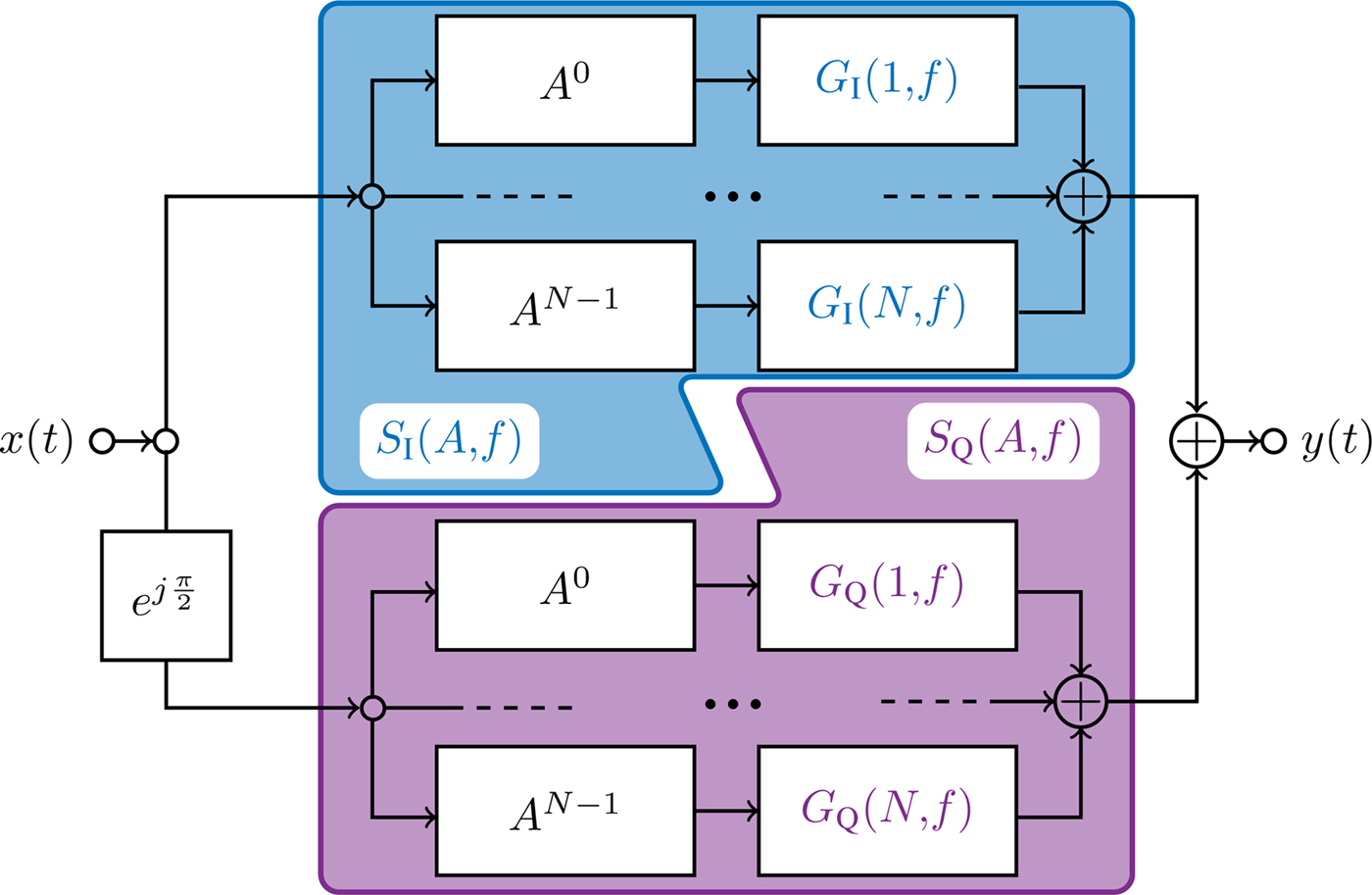
Fig. 1. Block schematic of the quadrature polynomial method.
III. STEADY-STATE BASE CODE MVTRAD
The main objective of our approach is to be able to simulate the multi-tone behavior of the device during the design process. Therefore, unlike in many other approaches, we cannot rely on measured TWT characteristics. This does not only limit the number of usable envelope models, but also requires a sound physical model as a basis. Specialized parametric steady-state codes such as MVTRAD offer the required functionality and performance.
MVTRAD is a 2.5D frequency-domain PIC code specialized on helix TWT. It computes the beam-wave interaction by modeling the electron beam as macro-particles in a two-dimensional plane, assuming rotational symmetry of the electromagnetic fields and the beam, while still taking the azimuthal movement of the particles into account. It is a parametric code, as the slow-wave circuit is represented by phase velocity and coupling impedance, which are generated, e.g. by full-wave simulation or analytical models. Large-signal continuous-wave computation can be carried out in less than a minute per frequency and power setting.
Although the particle motion is calculated in time domain, and therefore any non-linear mixing in the electron beam can in principle be simulated, the electromagnetic fields are only considered as known harmonic modes. While this indeed simplifies the field calculation for the determination of typical amplifier design characteristics, as they can be obtained by single-tone continuous-wave simulation, it complicates multi-tone simulation and a forteriori simulation of complex modulated signals. In principle, simulating a signal consisting of N tones in the operating band can be calculated using this approach by taking the greatest common divisor as the fundamental frequency with a sufficiently high number of harmonics. Of course, the number of time steps per period needs to be scaled accordingly, to have the same time resolution as in the single-tone computation case. As the greatest common divisor would generally be orders of magnitude smaller than the operating frequency – and for modulated signals in principle infinitely small – the use of codes like MVTRAD alone for multi-tone simulation is only possible in some special cases.
IV. MULTI-TONE EXCITATION
In a first step, the various envelope models are evaluated based on TWT measurements only, as this mitigates other error sources, such as inaccuracies in the underlying interaction model or its numerical implementation. In a second step, we replace the measured data by those from the steady-state simulation tool MVTRAD. This defines the proposed hybrid time- and frequency-domain approach, which combines the steady-state simulation of MVTRAD with the various envelope codes.
A) Measurement fitted models
The measurements are carried out on a reference communication Ku-band TWT. They include continuous-wave AM-AM and AM-PM measurements throughout the frequency band of interest, from which the model parameters of the three envelope codes are determined. They further include two-tone measurements with different frequency spacings. Although TWTs are usually not operated with two-tone signals, these can easily be understood and measured. In addition, they yield meaningful figures of merit. For these, even approximate formulas are available from literature. In addition, dual-tone signals represent the least challenging multi-frequency scenario. They are thus best suited to verify the intermodulation performance predicted by the approaches discussed here.
In the experiments, the two tones have equal input power, which is simultaneously altered in steps of 2 dB from small signal to saturation. A comparison of the simulated and measured intermodulation products for a constant center frequency f c and  $\Delta f = 100{\kern 1pt} \,{\rm MHz}$ is shown in Fig. 2. Only the upper side band is displayed, as the lower one is nearly indistinguishable. Both D 3 and D 5 show near-perfect agreement, as the amplifier characteristic is almost constant in the relevant band for this scenario, which can be seen in Fig. 3, and the input signal has a slowly changing amplitude. Even for a large offset of $\Delta f = 500{\kern 1pt} \,{\rm MHz}$, the SGC model performs just as well as the more involved methods, as can be seen from Fig. 4, which reports the power levels at f 2 and f 2 + Δf. Again, the overall agreement is good. However, in this case all models underestimate the power in one of the main tones by about 0.15–0.18 dB. This discrepancy might stem from the mismatch-induced gain ripple, which is not taken into account in the models.

Fig. 2. Intermodulation products at 100 MHz spacing.
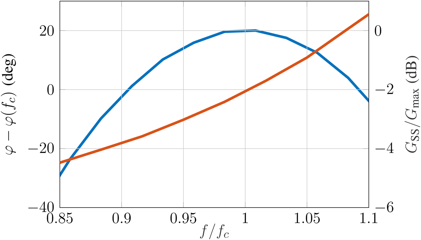
Fig. 3. Small-signal gain and non-linear phase shift at saturation over frequency.
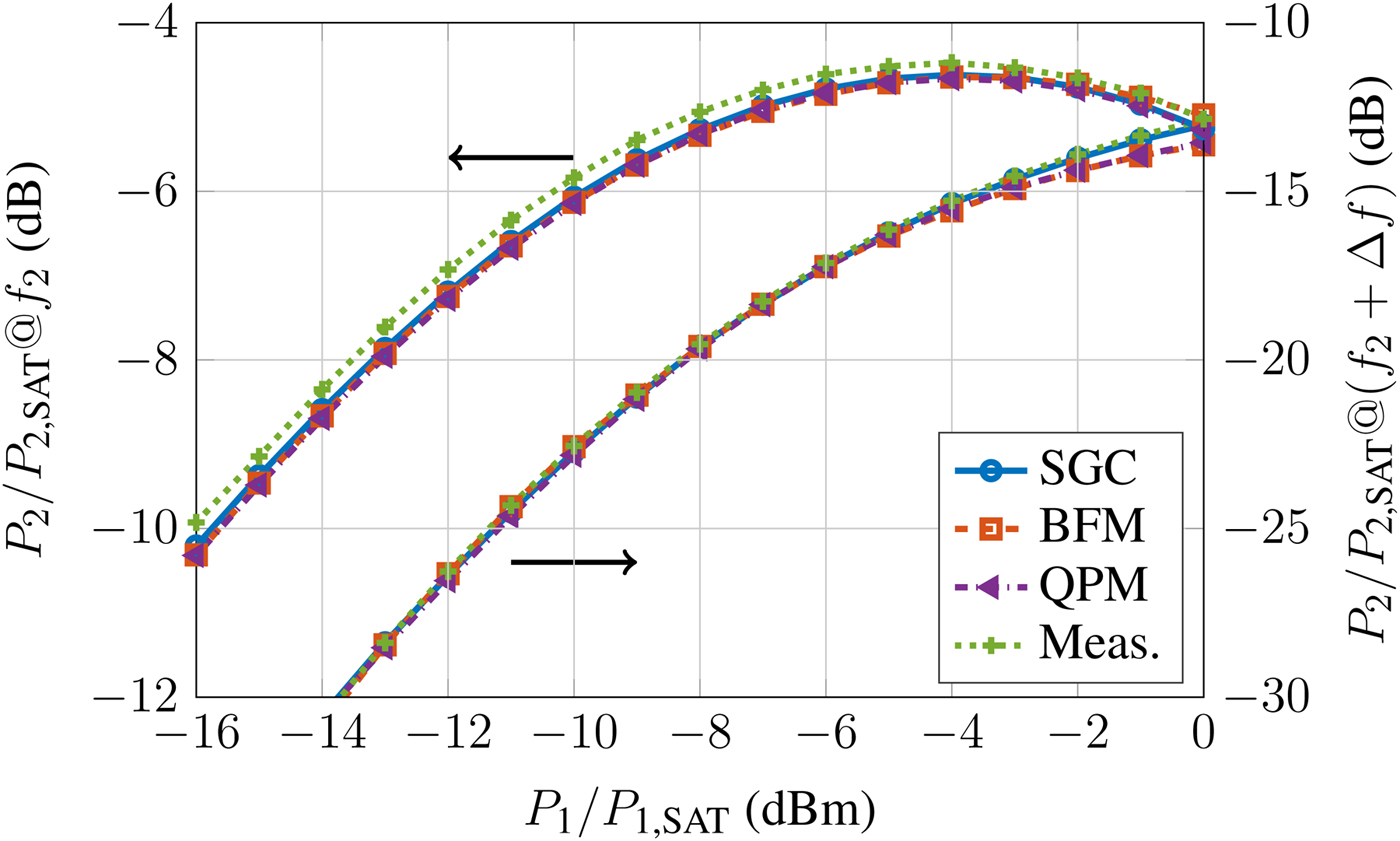
Fig. 4. Main tone and intermodulation product at 500 MHz spacing.
As another metric the phase transfer factor k T is shown versus input power in Figs 5–7 for different Δf. It is obtained here by setting P 1(f 1) = P 1(f 2) − 15 dB and by measuring the phase difference at f 1 when reducing P 1(f 2) by 1 dB. For better comparison, the absolute error Δk T between simulation and measurements is also shown. As the non-linear phase is strongly dispersive, the frequency-dependent models yield improved predictions.
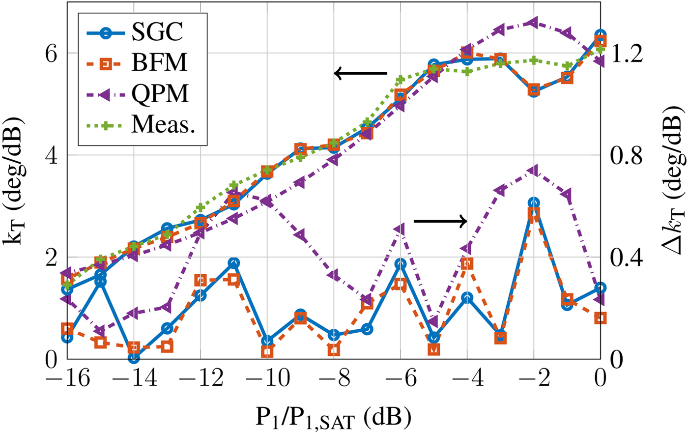
Fig. 5. Phase transfer factor at 5 MHz spacing.
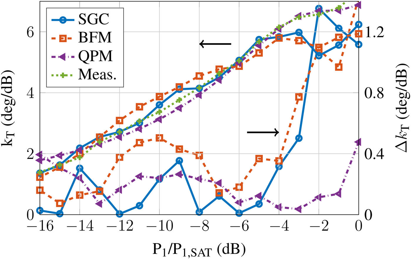
Fig. 6. Phase transfer factor at 200 MHz spacing.

Fig. 7. Phase transfer factor at 1 GHz spacing.
For  $\Delta f = 5{\kern 1pt} \,{\rm MHz}$ (Fig. 5), all models accurately predict the measured results. Figures 6 and 7 illustrate the advantage of adding frequency information to the model, especially close to saturation where the phase error increases rapidly. While for $\Delta f = 200{\kern 1pt} \,{\rm MHz}$ the error for both SGC and BFM rises above 1°/dB, it stays below 0.5°/dB for QPM. Similarly, for $\Delta f = 1{\kern 1pt} \,{\rm GHz}$ the error is largest for SGC and BFM. It exceeds 2.1°/dB, while remaining below 1.2°/dB for QPM. Although both QPM and BFM include dispersion information, only QPM significantly benefits from it. This is due to the strong fluctuation of the Bessel function fitting parameters over frequency, which yields a highly sensitive model. The polynomial parameters, in contrast, change far more gracefully, such that the required interpolation between fitting points is significantly improved.
B) MVTRAD fitted models
To evaluate the models inside the full simulation chain including the interaction simulation, an MVTRAD reference model has been generated and fitted as closely as possible to the measured TWT. The measured results are adjusted by the difference in saturated input power between the MVTRAD model and the measured data to enable comparison.
Different two-tone scenarios close to saturation are measured and calculated with both the hybrid models and MVTRAD alone. For this, CW output power and absolute phase versus input power (from small signal to 10 dB into overdrive in 1 dB steps) and frequency (in 100 MHz steps inside the band of interest) are simulated in MVTRAD beforehand. For the hybrid SGC model, the signals are then evaluated with respect to their frequency content and the center frequency is taken as the model reference frequency. For the other two models, as the possible intermodulation frequencies are known, the TWT data at these frequencies are extracted and taken as reference for the fitting.
Figure 8 reports the resulting power spectrum for a two-tone signal with  $\Delta f = 100\,{\kern 1pt} {\rm MHz}$ at around 0.5 dB input back-off (IBO). It can be seen that due to the small spacing between the tones, all models closely match both the MVTRAD and the measurement results. Only at 3 Δf small errors can be seen, mainly caused by inaccuracies in the reference MVTRAD model. For a large spacing of $\Delta f = 500{\kern 1pt} \,{\rm MHz}$, the results are shown in Fig. 9. Here, P 2(f 2) is overestimated by up to 0.2 dB by each of the models as well as by MVTRAD, and P 2(f 1) even by as much as 0.5 dB. Still, the frequency dependency helps improving the estimation, as can be seen at f 1 − Δf. While the SGC model overestimates the power by 1.2 dB, using the QPM lowers the error to <0.5 dB, which is the same as in MVTRAD. At the higher frequencies, all models show similar errors.
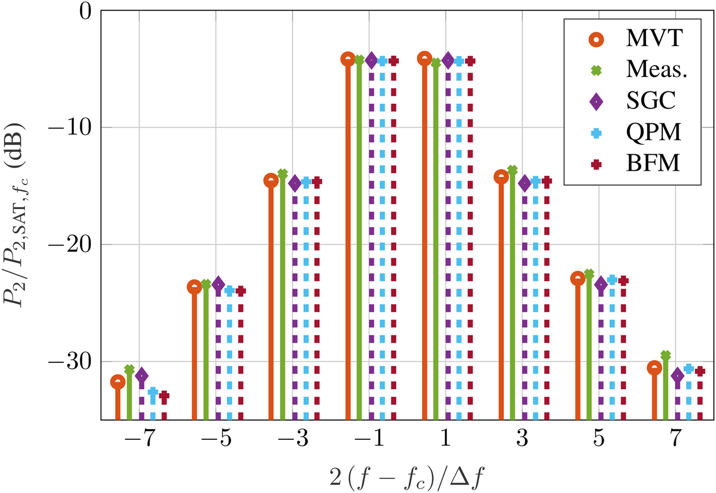
Fig. 8. Two-tone signal around f c with Δf = 100 MHz at 0.5 dB IBO.
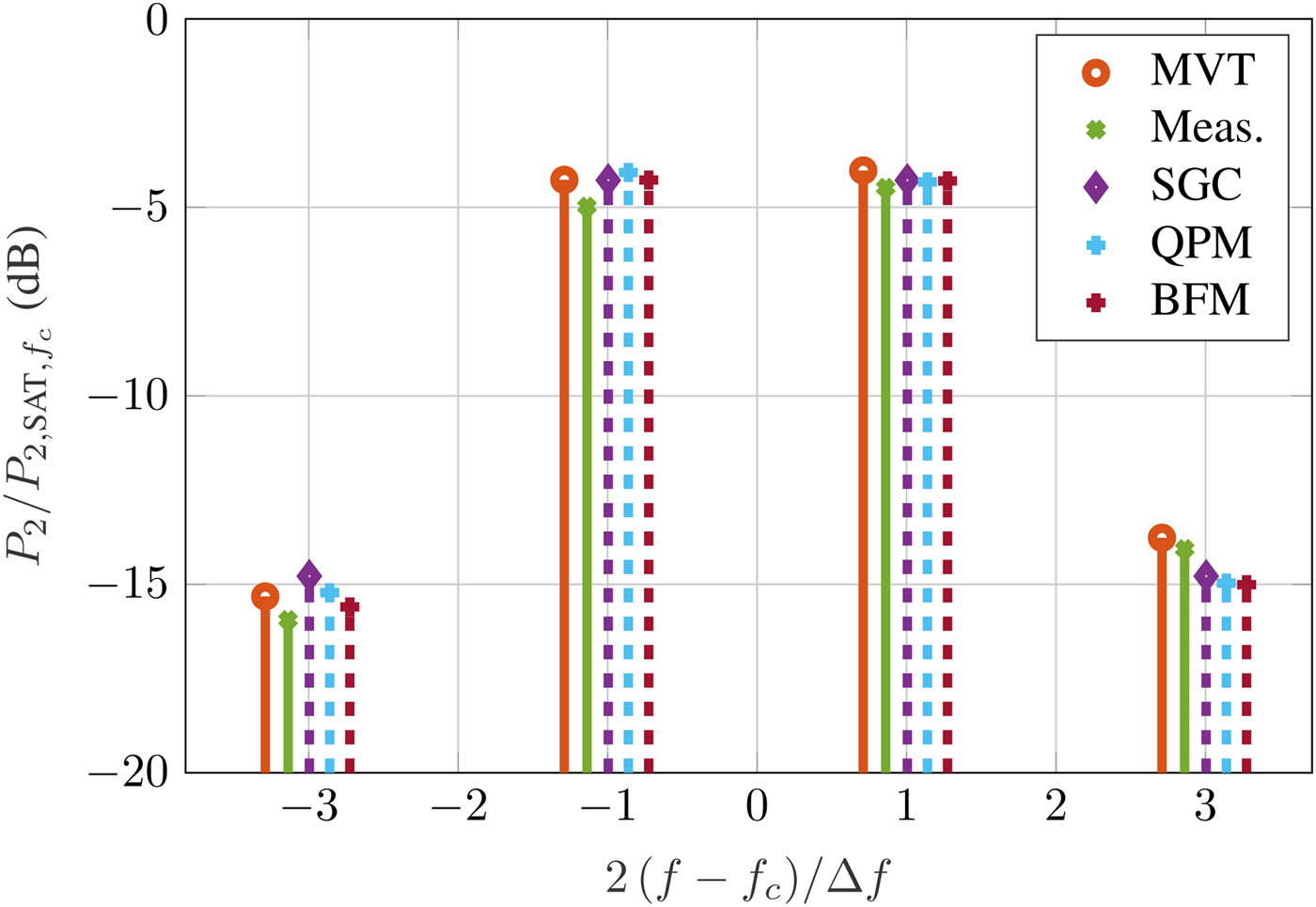
Fig. 9. Two-tone signal around f c with  $\Delta f = 500{\kern 1pt} \,{\rm MHz}$ at 0.5 dB IBO.
In Figs 8 and 9, the center frequency corresponds to the band center, where the dispersion is small. To show the applicability of the models for more dispersive cases, two more scenarios are investigated. In Fig. 10, the center frequency is shifted down by 5% and Δf is set to 500 MHz. At the main frequencies, the results of all models are close to each other and to the measurements. At the lower side band, due to the input and output coupler and limited calibration, no reliable measurements are available. Still, one can compare the envelope codes to MVTRAD. As can be seen, the power spectrum from MVTRAD is slightly more asymmetric than in the previous cases, as the device is more dispersive. In contrast, the SGC model always results in a symmetric output spectrum for a symmetric two-tone input and thus yields a large error of about 1.5 dB. Both QPM and BFM are significantly closer. For the upper side band, all hybrid models are similarly far away from both measurements and MVTRAD, the error being around 1 dB. Finally, Fig. 11 shows the results for a center frequency at the lower band edge and  $\Delta f = 200{\kern 1pt} \,{\rm MHz}$. Again, BFM and QPM yield some improvements at the side bands, reducing the error from 0.7 dB for SGC to <0.3 dB at f 2 + Δf. The power at f 1 − Δf can only be compared to MVTRAD, but also here the dispersive models are significantly closer than SGC, lowering the error from 1.2 to 0.5 dB.
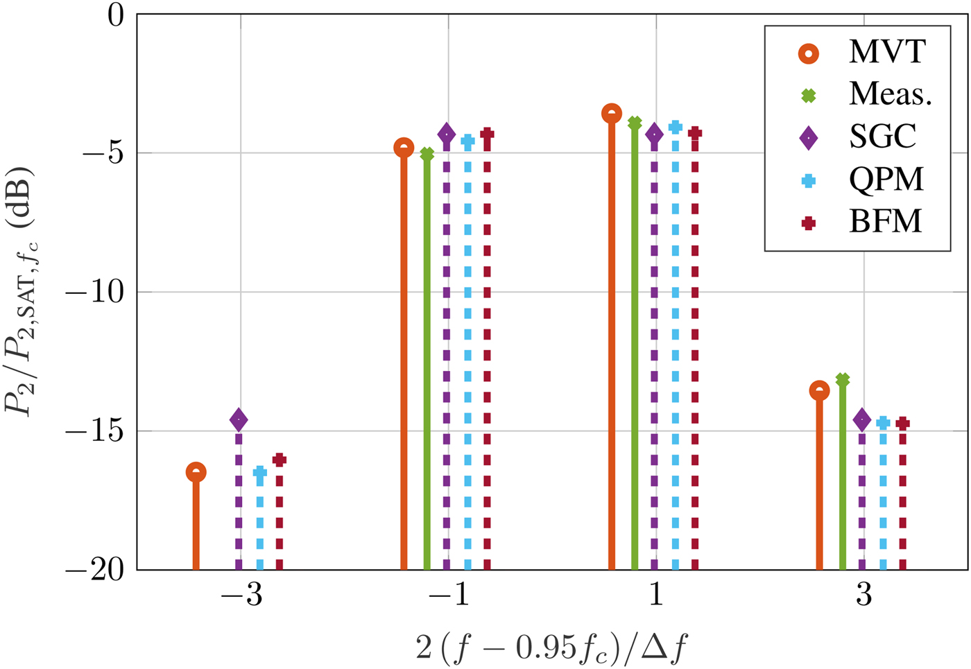
Fig. 10. Two-tone signal around 0.95 f c with  $\Delta f = 500{\kern 1pt} \,{\rm MHz}$ at 0.5 dB IBO.
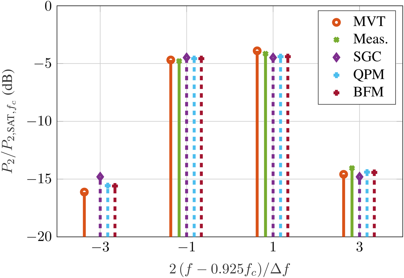
Fig. 11. Two-tone signal at lower band edge 0.925 f c and  $\Delta f = 200{\kern 1pt} \,{\rm MHz}$ at 0.5 dB IBO.
The MVTRAD results are generated by calculating the greatest common divisor of the tones and scaling the time resolution according to the number of harmonics taken into account. This increases the total interaction simulation time, depending on the common fundamental frequency, to up to 15 h for the presented scenarios. As the envelope simulation itself takes far less than a minute, the computation time for the hybrid approach is mainly determined by the frequency-domain part. It can be reduced to about 3 h by parallelization. However, most of the table is not used for the shown results. Considering only frequencies required for the models in each specific frequency setting would reduce the total computation time to a few minutes.
V. MODULATED SIGNALS
Two-tone excitation, while popular for amplifier characterization, does not always provide a complete picture. A strong limitation follows from the fact, that the initial phase relations between the two tones do not have any influence on the power spectrum. TWTs are also usually operated with complex modulation. Therefore, it is useful to look at eye diagrams, constellation diagrams and other communications-related metrics to characterize the tube in realistic operating conditions.
For a full validation using such signals, a set of specified symbol sequences is periodically repeated. Each periodic sequence is then translated to a QPSK-modulated signal. The baseband signal is generated with a pulse-forming filter, such as a root-raised cosine filter, and subsequently upconverted to the carrier frequency to generate the amplifier RF input signal. The filter is specified by the roll-off factor α, describing the frequency excess of the filter, and by its symbol span ξ. While α is a system-dependent parameter usually chosen between 0.25 and 0.35, ξ denotes the number of symbols taken into account for smoothing the rectangular pulse sequence to limit the bandwidth and has a strong influence on the amplitude distribution of the signal. Values above six have been found to have no significant influence on the amplitude histogram, while values below that strongly distort it. For the modulation scenario to have a physical setting, a data rate R c has to be additionally defined to set the bandwidth.
In principle, a full eye-diagram generation for a QPSK modulation requires a Monte-Carlo study. While this is possible in measurements or time-domain simulation using envelope codes, it would result in an infinite number of frequencies in a frequency-domain simulation or a very large simulation time in any full-wave code. A program like MVTRAD or even a full-wave PIC code such as CST Particle Studio thus cannot be employed for comparison.
To characterize amplifiers, the number of meaningful sequences can be significantly reduced. As one can neglect channel noise, for instance, the simulated eye diagram is purely deterministic. The number of sequences needed to describe the full eye diagram then only depends on the modulation type and the pulse-forming filter. Using a filter span of six means that for each symbol the information of in total seven symbols is taken into account. As the eye diagram depicts the effect of all possible symbol transitions, a large number of sequences is needed. In the linear part of the amplifier characteristic, the inphase and the quadrature channel are independent of each other and do not cause significant intermodulation. In the non-linear case, however, they cannot be considered separately. Fixing the inphase channel, we only have to take a subset of sequences into account. An infinite periodic repetition of a seven-symbol sequence typically consists of more than one seven-symbol sequence. An algorithm has been written, which generates a set of sequences that includes as many other sequences as possible. This results in only 20 sequences to be simulated, consisting of all possible sequences in one channel for a fixed second channel. Taking into account that the inverse bit sequence is generated by a 180° phase shift, the number of simulation runs can be halved. As one of these 10 sequences necessarily consists only of either zeros or ones, which yields a quasi continuous-wave signal, it can be discarded. This sequence reduction is shown in Fig. 12. In a linear setting, the full eye diagram can be generated by these nine seven-symbol sequences. Of course, as we have a non-linear amplifier, it is not complete, but we have a selection of sequences with the highest possible information content, which renders a large portion of the eye diagram. If the other channel is chosen with the same periodicity (but possibly from another sequence or at least a shifted version of the chosen sequence), the total complex signal is still periodic and therefore has a discrete spectrum. Finally, the data rate and roll-off factor are chosen according to
 $$\Delta f = \displaystyle{{R_c} \over {(1 + \alpha ) \cdot (\xi + 1)}},$$
where Δf denotes the spacing between the discrete frequencies and is chosen to be 50 MHz. The carrier frequency is chosen such that all discrete frequency components are multiples of Δf. The total frequency band containing significant information can then be estimated to 350 MHz.
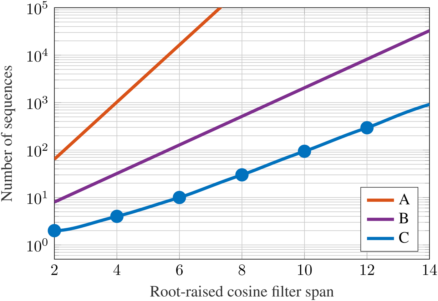
Fig. 12. Reduction of the number of sequences to compute by periodic sequence repetition. (a) All symbol permutations. (b) All combinations in one channel. (c) Reduced number of sequences.
The generated signal is periodic with T 0 = 1/Δf. Therefore, the complex Fourier coefficients with fundamental frequency Δf are calculated by time windowing with T 0 and using a discrete Fourier transform. For MVTRAD, the complex phasor description of the Fourier coefficients of 80 harmonics of Δf representing the operating band and possible intermodulation products, as well as the corresponding second harmonic frequencies around 2f c are computed. As this results in a large total number of harmonics and therefore a large number of time steps within a base period, the computation time is around 4 days per sequence. Using the phasor Fourier sum of the resulting amplitudes and phases, the resulting time-domain signal is reconstructed. After down-conversion and receive-filtering, the eye diagram can be calculated. In the following, the combined SGC-MVTRAD model is compared to a full frequency-domain PIC interaction simulation with MVTRAD. In this example, we chose an IBO of only 2 dB for strong intermodulation.
Figures 13 and 14 exemplarily show the power spectrum and envelope, generated using the Hilbert transform, of the time-domain signals for one sequence, both from MVTRAD and the SGC-MVTRAD combined approach. From the power spectrum, it can be seen that the overall agreement is excellent for the main input frequencies and still very good for the intermodulation products. At the lower frequencies, the envelope approach overestimates the power. Translating the power and phase results from MVTRAD to time domain, we see good agreement between the signals from SGC and MVTRAD, when only frequency components up to f c + 40 Δf are considered. Using the full spectrum as calculated in MVTRAD, the modulus of the analytic signal representation looks slightly different, as the second harmonic components around 2f c distort the signal. These can in general not be seen from the SGC model, but as the signal is low-pass filtered on the demodulation side, they are irrelevant for the investigation.

Fig. 13. Output power spectrum of an examplary QPSK sequence.

Fig. 14. Output waveform comparison of an examplary QPSK sequence. (a) MVTRAD results, considering components around f c and 2f c. (b) MVTRAD results, only considering components around f c. (c) SGC model results.
Figures 15 compares the eye diagrams obtained with MVTRAD and with the combined SGC-MVTRAD approach. The eye from the envelope simulation is slightly more blurred, so that both the vertical and the horizontal eye opening are 6% smaller. Still, the overall agreement between both diagrams is good.
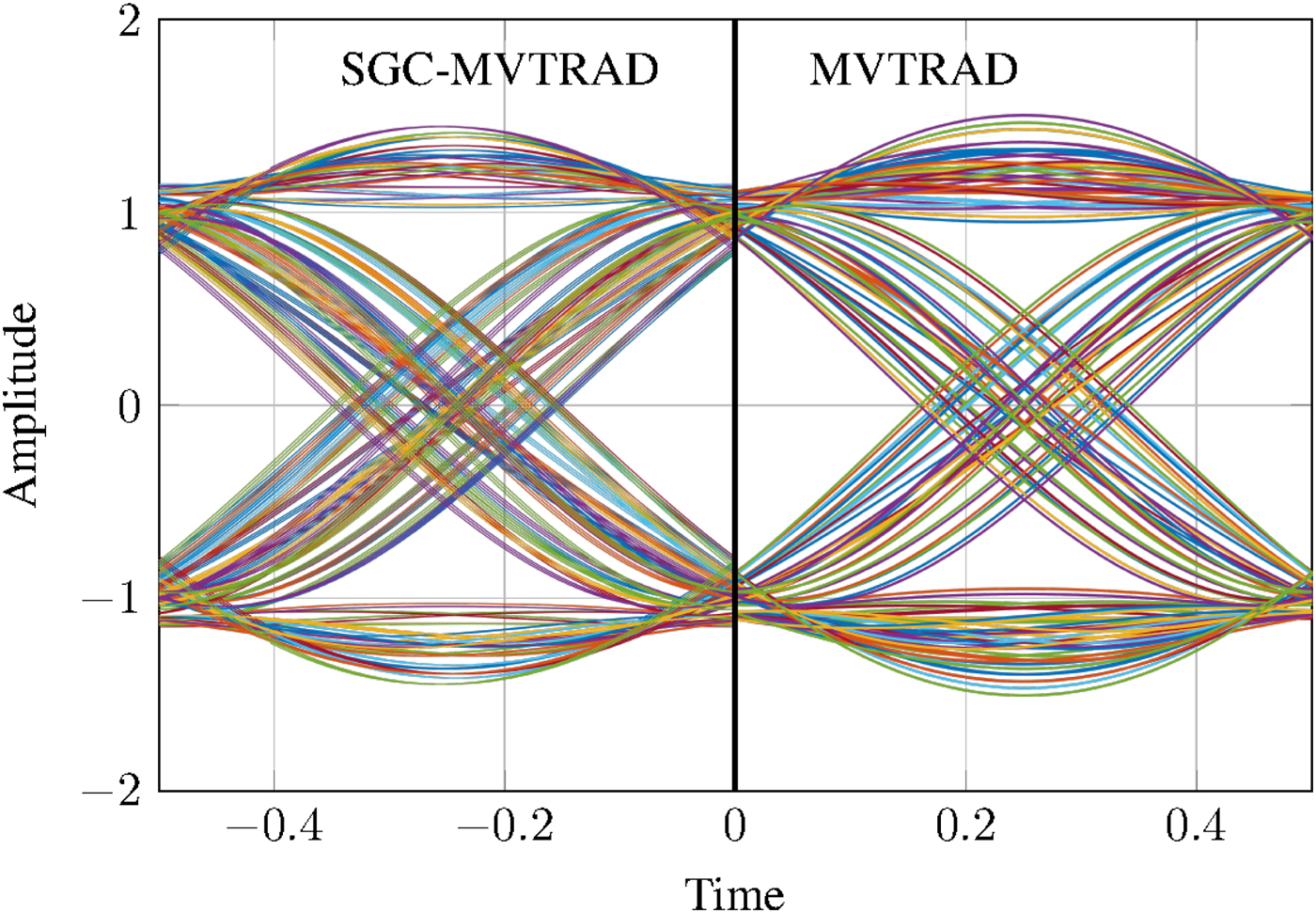
Fig. 15. Quadrature eye diagrams from SGC and MVTRAD.
VI. CONCLUSION
In this work, three different models have been evaluated concerning their applicability in a hybrid time- and frequency-domain TWT simulation. For this purpose, they have been compared to measurements and simulation results in a variety of multi-tone scenarios. It has been shown that for a real communications TWT at typical operating conditions and practically relevant frequency spacings, the basic SGC model using the Hilbert transform is sufficient to predict the powers at the intermodulation levels. An extension using multiple AM-AM and AM-PM results over a range of frequencies only improves the estimation of the intermodulation products for selected, more dispersive scenarios. The prediction of the phase transfer, on the other hand, can benefit from the more sophisticated models. Additionally, a sequence reduction scheme for the approximate generation of modulated signals has been presented. It enables the meaningful comparison of the envelope models with interaction simulation and yields high accuracy.
ACKNOWLEDGEMENT
The authors wish to acknowledge funding and support of this work by the German Aerospace Center (DLR) on behalf of the German Federal Ministry of Economics and Technology (BMWi) under research contract 50YB1508.
 Djamschid Safi received the M.Sc. degree in Electrical Engineering at the Technische Universität Hamburg-Harburg, Germany in 2015. He is currently working towards his Ph.D. at the Institut für Hochfrequenztechnik, Technische Universität Hamburg-Harburg, Germany, in the field of traveling-wave tubes. His research interests include modeling and interaction simulation of traveling-wave tubes, especially related to communication systems.
 Sascha Meyne received the Dr.-Ing. degree in 2016 from the Technische Universität Hamburg-Harburg, Hamburg, Germany. He is currently working at the Institut für Hochfrequenztechnik at the Technische Universität Hamburg-Harburg, Hamburg, Germany, in the field of traveling-wave tubes. His research interests include modeling of radio frequency components, interaction simulation, and related numerical methods.
 Philip Birtel received the Dipl.-Ing. degree in Electrical Engineering from the Technische Universität Braunschweig, Braunschweig, Germany, in 2004 and the Ph.D. degree in Electrical Engineering from the Technische Universität Hamburg-Harburg, Hamburg, Germany, in 2011. He is involved in the modeling and design of space TWTs at Thales Electronic Systems, Ulm, Germany.
 Arne F. Jacob received the Dr.-Ing. degree in 1986 from the Technische Universität Braunschweig, Germany. From 1986 to 1988 he was a Fellow at CERN, the European Organization for Nuclear Research, Geneva, Switzerland. In 1988, he joined Lawrence Berkeley Laboratory, University of California at Berkeley for almost 3 years as a Staff Scientist at the Accelerator and Fusion Research Division. In 1990, he became a Professor at the Institut für Hochfrequenztechnik, Technische Universität Braunschweig. Since October 2004, he has been a Professor at the Technische Universität Hamburg-Harburg, Hamburg, Germany, where he heads the Institut für Hochfrequenztechnik. His current research interests include the design, packaging, and application of integrated (sub-)systems up to millimeter frequencies, and the characterization of complex materials.


