


1. Introduction
Vertically distributed wall-source plumes, the flow driven by a uniform vertical wall source of buoyancy, frequently occur within buildings. For example, in winter, downward convection produced at the surface of cold glazing, or in summer, upward convection on warm glazing, shading devices or walls that have absorbed solar radiation. Of particular interest to practitioners is the resulting temperature stratification that develops within a space as a result of these types of flows, particularly tall spaces such as atria. In Part 1 (Parker et al. Reference Parker, Burridge, Partridge and Linden2021) of this work we considered a distributed wall-source plume in an unconfined environment by creating a uniform vertical wall source of buoyancy by forcing relatively dense salt water through a porous wall. Here we enclose the apparatus used in Part 1 and perform density measurements to investigate the resulting ambient buoyancy stratification that develops as a result of a distributed wall-source plume in both a confined unventilated environment and a confined ventilated environment.
When a uniform vertically distributed buoyancy source is placed within a confined environment the buoyant plume reaches the top surface and spreads across it creating a layer of buoyant fluid and a density interface between the buoyant and ambient fluid (Baines & Turner Reference Baines and Turner1969), as illustrated in figure 1. This is the ‘filling box’ which establishes a stable stratification within the space. As a result of entrainment, increasingly buoyant fluid continues to accumulate at the ceiling and the position of the density interface moves vertically downwards at a rate determined by the volume flux of the plume at the height of the interface. This falling interface is traditionally referred to as the first front. The time-evolution of the height of the first front of a filling box was first determined by Baines & Turner (Reference Baines and Turner1969) for the case of a turbulent axisymmetric plume filling an unventilated box. This theory was later adapted to a distributed wall-source plume filling a box by Cooper & Hunt (Reference Cooper and Hunt2010). This analysis was extended to account for the additional source volume flux (such as in the current experimental method) by Kaye & Cooper (Reference Kaye and Cooper2018).
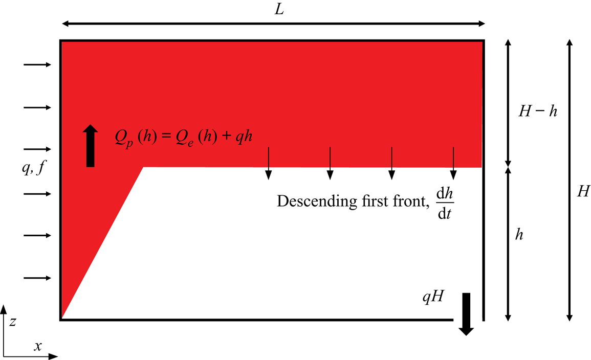
Figure 1. Schematic of the unventilated distributed wall-source plume with a finite source volume flux  $q$ and buoyancy flux $f$ per unit area, where the box is connected to the exterior environment by an open vent at the bottom of the box. The rate of descent of the first front must balance the plume volume flux entering the stratified region and the additional source volume flux within the stratified region, i.e. $\mathrm{d} h/\mathrm{d} t=-(Q_p+q(H-h))L^{-1}$, where we assume that the plume width is much smaller than $L$.
$L$.
By adapting the filling box model of Germeles (Reference Germeles1975), Cooper & Hunt (Reference Cooper and Hunt2010) developed a numerical model of the evolving stratification of the ambient. The ambient stratification was assumed to develop such that the distributed wall-source plume continually lays down a thin layer of fluid at the top of the confined box. Although Cooper & Hunt (Reference Cooper and Hunt2010) observed qualitative agreement between experiments and the numerical predictions outlined above they did not find quantitative agreement. In particular, the step change in buoyancy that is assumed at the first front in the numerical model was not observed in experiments.
Stratification profiles of the filling box problem have also been measured in McConnochie & Kerr (Reference McConnochie and Kerr2015), Caudwell, Flór & Negretti (Reference Caudwell, Flór and Negretti2016) and Bonnebaigt, Caulfield & Linden (Reference Bonnebaigt, Caulfield and Linden2018). Caudwell et al. (Reference Caudwell, Flór and Negretti2016) found the numerical model of Cooper & Hunt (Reference Cooper and Hunt2010) was largely unsuccessful in predicting the quantitative profiles, even if an adaptive entrainment coefficient is used in the model. Bonnebaigt et al. (Reference Bonnebaigt, Caulfield and Linden2018), however, was able to model the stratification by assuming a peeling model (originally developed by Hogg et al. (Reference Hogg, Dalziel, Huppert and Imberger2017) for a filling-basin model of an inclined gravity current) where the plume velocity and buoyancy profiles are assumed to have linear, as opposed to top-hat, profiles and fluid at the outer edge of the plume peels off and moves to its neutral buoyancy height within the stratified layer, without further mixing occurring. Bonnebaigt et al. (Reference Bonnebaigt, Caulfield and Linden2018) assumed an ideal source with no wall shear stress in their model. Herein, we extend the model of Bonnebaigt et al. (Reference Bonnebaigt, Caulfield and Linden2018) by accounting for the effects of the wall shear stress, the source volume flux and the measured buoyancy distribution of volume flux within the plume.
The behaviour of distributed wall-source plumes in ventilated spaces was examined by Cooper & Hunt (Reference Cooper and Hunt2010). However, akin to their experience with the filling box, Cooper & Hunt (Reference Cooper and Hunt2010) found that the numerical model was not able to predict the quantitative transient or steady-state ambient buoyancy profile. Gladstone & Woods (Reference Gladstone and Woods2014) studied the ventilation of a vertically distributed line source showing that there was no net plume entrainment in the stratified region in steady state. Gladstone & Woods (Reference Gladstone and Woods2014) suggested that in such a system the local entrainment and peeling (therein ‘detrainment’) is controlled by the local difference in the mean plume and ambient buoyancy and, since the system is in steady state, it was suggested that this local difference of buoyancy should be independent of height. They validated this insight experimentally.
The aim of this second part of our study is to examine a confined distributed wall-source plume based on the porous wall method of Cooper & Hunt (Reference Cooper and Hunt2010). Herein, we examine the evolution of this plume both in an unventilated ‘filling box’ and in a ventilated ‘emptying–filling box’ using the method of dye attenuation to determine the evolving and steady-state ambient stratification. This part is organised as follows. In § 2 we review the filling box models of Cooper & Hunt (Reference Cooper and Hunt2010) and Bonnebaigt et al. (Reference Bonnebaigt, Caulfield and Linden2018), the emptying–filling box theory of Gladstone & Woods (Reference Gladstone and Woods2014) and present our theory. The experimental methods are described in § 3. The results of the buoyancy measurements examining the developing ambient stratification of the filling box and emptying–filling box experiments are presented in §§ 4.1 and 4.2, respectively. Inspired by industrial needs and the building ventilation application, in § 5.1 we describe a methodology for the creation of a desired linear buoyancy profile, and therefore temperature stratification, within a room via a prescribed uniform wall heat flux and in § 5.2 we consider the implications for a typical atrium where absorbed solar radiation creates a heated glass wall. Finally, conclusions are drawn in § 6.
2. Theory
2.1. Unventilated confined space
Based on the model of Baines & Turner (Reference Baines and Turner1969), Kaye & Cooper (Reference Kaye and Cooper2018) modelled the first front evolution,  $h(t)$ (see figure 1), by balancing the downward motion of the first front with the plume volume flux in the opposite direction. This can be expressed as
 \begin{equation} \frac{\mathrm{d} h}{\mathrm{d} t}=-\frac{1}{L}(Q_p(h)+q(H-h))=-\frac{1}{L}(Q_e(h)+qH), \end{equation}
where  $Q_p(z)$ is the total volume flux per unit length (in the spanwise direction), $Q_e(z)$ is the cumulative entrained volume flux per unit length, $q$ is the source volume flux per unit area, $H$ is the total height of the wall and $L$ is the width of the box. This work is primarily concerned with flows on sufficiently large scales to be considered turbulent. The turbulent plume theory discussed in Part 1 may then be used to model the volume flux by assuming that the laminar region is negligible. By assuming that the cumulative entrained volume flux follows the ideal plume solution determined in Part 1 and ignoring the source volume flux, i.e. $q=0$, (2.1) may be solved to give
 \begin{equation} \frac{h(t)}{H}=\left(1+\frac{1}{4}\left(\frac{4}{5}\right)^{1/3}\left(\frac{f}{1+\dfrac{4C}{5\alpha}}\right)^{1/3}\alpha^{2/3}L^{-1}H^{1/3}t\right)^{-3}, \end{equation}
where  $f$ is the source buoyancy flux per unit area and $C$ is the wall skin friction coefficient. By comparing measurements of $h(t)$ with the right-hand side of (2.2) a best-fit entrainment coefficient may be determined.
Due to the accumulation of buoyant fluid within the ambient, the equations for the unstratified case, given in Part 1, are modified to include a stratified ambient environment where the buoyancy of the ambient fluid is defined by  $b_e=g(\rho _a-\rho _e)/\rho _a$, where $\rho _e=\rho _e(z,t)$ is the density of the ambient fluid and $\rho _a$ is the constant initial ambient fluid density. The buoyancy of the plume fluid is now defined relative to the varying ambient density, $b(z, t)=g(\rho _e-\rho )/\rho _a$, where $\rho$ is the plume density.
The plume conservation equations for volume flux  $Q$, specific momentum flux $M$ and buoyancy flux $F$ per unit length now become
 \begin{gather} \frac{\mathrm{d} Q_p}{\mathrm{d} z}=\alpha\frac{M}{Q_p}+q, \end{gather}
 \begin{gather}\frac{\mathrm{d} M}{\mathrm{d} z}=\frac{\theta F Q_p}{M}-C\left(\frac{M}{Q_p}\right)^2, \end{gather}
 \begin{gather}\frac{\mathrm{d} F}{\mathrm{d} z}=f-qb_e-Q_p\frac{\partial b_e}{\partial z}=f-qb_e-Q_pN_e^2, \end{gather}
where  $N_e^2\equiv \partial b_e/\partial z$ is the buoyancy frequency of the ambient and $\theta$ is the similarity coefficient, which we take as unity from hereon in.
Cooper & Hunt (Reference Cooper and Hunt2010) developed a numerical filling box model of the evolving stratification. The ambient stratification was assumed to develop such that the distributed wall-source plume continually lays down a thin layer of fluid, of buoyancy  $f H/Q_p(H)$, at the top, $z=H$, of the confined box. Diffusion and the effect of the aspect ratio of the box were neglected and it was assumed that the time scale of the plume to fill the box was much greater than the time scale of the plume to rise through the box, i.e.
 \begin{equation} \frac{HL}{Q_p(H)}\frac{W(H)}{H}=\frac{4L}{3\alpha H}\gg 1, \end{equation}
where  $W$ is the characteristic vertical velocity of the plume defined by $W=M/Q_p$. Consequently, the ambient buoyancy evolves according to the advection equation
 \begin{equation} \frac{\partial b_e}{\partial t}=\frac{Q_p}{L}\frac{\partial b_e}{\partial z}. \end{equation}
For each time step, (2.3), (2.4) and (2.5) are solved numerically, with the assumption that  $q=0$, and the ambient buoyancy, $b_e$, is updated according to (2.7). Cooper & Hunt (Reference Cooper and Hunt2010) found that this model was unable to effectively model experimental observations of a filling box in the presence of a distributed wall-source plume. Caudwell et al. (Reference Caudwell, Flór and Negretti2016) used the above model of Cooper & Hunt (Reference Cooper and Hunt2010) by incorporating an adaptive entrainment coefficient that was empirically determined from plume velocity measurements, which partially accounted for the laminar region of the flow, but was unsuccessful in matching experimental observations.
In the peeling model developed by Bonnebaigt et al. (Reference Bonnebaigt, Caulfield and Linden2018), originally described by Hogg et al. (Reference Hogg, Dalziel, Huppert and Imberger2017) for an inclined gravity current entering a basin, an ideal source with no shear stress was assumed. Here, we describe the general peeling method used by Bonnebaigt et al. (Reference Bonnebaigt, Caulfield and Linden2018), without restricting attention to the ideal case, so that the results of a non-ideal source considered in Part 1 may be applied. Before we describe the peeling method used by Bonnebaigt et al. (Reference Bonnebaigt, Caulfield and Linden2018) it is convenient to introduce dimensionless variables for which we follow the non-dimensionalisation of Cooper & Hunt (Reference Cooper and Hunt2010) (as used by Bonnebaigt et al. Reference Bonnebaigt, Caulfield and Linden2018)
 \begin{equation} \left. \begin{gathered} \xi=zH^{-1},\quad \tau=\alpha^{2/3}H^{1/3}L^{-1}f^{1/3}t,\quad \delta_e=\alpha^{2/3}H^{1/3}f^{-2/3}b_e,\\ \mathscr{Q}=\alpha^{-2/3}H^{-4/3}f^{-1/3}Q,\quad \mathscr{M}=\alpha^{-1/3}H^{-5/3}f^{-2/3}M,\quad \mathscr{F}=H^{-1}f^{-1}F, \end{gathered} \right\} \end{equation}
where  $Q$ may be either the total volume flux per unit length $Q_p$ or the cumulative entrained volume flux per unit length $Q_e$. We denote the non-dimensional height of the first front as $\xi _0$, so that the volume flux and characteristic buoyancy of the plume at the height of the first front are given as functions of time by $\mathscr {Q}(\xi _0(\tau ))$ and $\delta _0(\xi _0(\tau ))=\mathscr {F}(\xi _0(\tau ))/\mathscr {Q}(\xi _0(\tau ))$, respectively.
Since peeling fluid is assumed to settle without mixing, the cumulative buoyancy distribution of volume flux at the first front must be incorporated into the model. The cumulative buoyancy distribution of volume flux  $Q_{b}(b^*,z)$ is defined, for a given height, as the volume flux of the plume with plume fluid buoyancy greater than a given buoyancy, $b^*$. We express the non-dimensional cumulative buoyancy distribution of volume flux as $\mathscr {Q}_{\delta }(\delta ^*,\xi )$. For example, Bonnebaigt et al. (Reference Bonnebaigt, Caulfield and Linden2018) considered linear plume velocity and buoyancy profiles given by
 \begin{equation} \frac{\mathscr{W}}{\mathscr{W}_m}=\begin{cases} 1-\chi, & \chi<1,\\ 0, & \chi>1, \end{cases} \quad \mathrm{and}\quad \frac{\delta}{\delta_m}=\begin{cases} 1-\chi, & \chi<1,\\ 0, & \chi>1, \end{cases} \end{equation}
where  $\mathscr {W}$ is the non-dimensional plume velocity and $\chi =x/R$ is the non-dimensional cross-stream distance, where $R$ is the characteristic plume width, and the subscript $m$ denotes maximum. For these profiles the cumulative buoyancy distribution of volume flux at the position of the first front is given by
 \begin{equation} \frac{\mathscr{Q}_{\delta}(\delta^*,\xi_0)}{\mathscr{Q}(\xi_0)}=\left\{\begin{array}{@{}ll} 1-\left(\dfrac{2\delta^*}{3\delta_0}\right)^2, & \dfrac{\delta^*}{\delta_0}<\dfrac{3}{2},\\ 0, & \dfrac{\delta^*}{\delta_0}>\dfrac{3}{2}, \end{array} \right. \end{equation}
where we have used the result that  $\delta _m(\xi _0)=3\delta _0/2$ since it is useful to express $\mathscr {Q}_{\delta }$ in terms of the characteristic plume buoyancy. The height $\xi ^*$ at which the fluid of buoyancy $\delta ^*$ is located is then calculated by finding the cumulative volume flux of fluid of buoyancy greater than $\delta ^*$. This may be expressed by
 \begin{equation} \xi^*(\delta^*,\tau)=1-\int_0^{\tau}\mathscr{Q}_{\delta}\left(\delta^*,\xi_0(\tau)\right)\,\mathrm{d} \tau. \end{equation}
Bonnebaigt et al. (Reference Bonnebaigt, Caulfield and Linden2018) accounted for the additional buoyancy effects on the plume within the stratified region by adding the source buoyancy to the buoyancy profile calculated above at each height. This additional buoyancy,  $\Delta \delta (\xi ,\tau )$, at each height and time may be expressed by
 \begin{equation} \Delta\delta(\xi,\tau)=\max\left(\tau-\tau_0(\xi),0\right) \end{equation}
where  $\tau _0(\xi )$ is the time at which the first front reaches $\xi$. The final buoyancy profile is thus given by $\delta ^*(\xi ^*,\tau )+\Delta \delta (\xi ^*,\tau )$. We compare this model with experiments in § 4.1 and suggest some adaptations to the ideal plume model shown above and considered by Bonnebaigt et al. (Reference Bonnebaigt, Caulfield and Linden2018).
2.2. Ventilated confined flow
In this section we consider the ventilation of a system where openings are placed at the top and bottom of the box (see diagram in figure 2). This type of ventilation is commonly called displacement ventilation (Linden, Lane-Serf & Smeed Reference Linden, Lane-Serf and Smeed1990), whereby buoyant fluid is extracted from the top opening and fresh ambient, i.e. relatively dense, fluid is introduced from the exterior environment through the bottom opening. A stable stratification is therefore produced within the ambient fluid. The buoyant fluid from the top opening may be extracted naturally, where the ventilation is driven only by the hydrostatic pressure difference between the box and the external environment, or by forced ventilation. Herein the ventilation is forced at a flow rate of  $Q_v+qH$ through the top opening which results in a ventilation flow rate of $Q_v$ per unit spanwise length through the bottom opening. Assuming that the ventilation flow rate is smaller than the flow rate of the plume at the top of the box, the first front reaches a steady state at the height at which the ventilation flux matches the cumulative entrained volume flux, i.e. the height $h$ such that $Q_e(h)=Q_v$. Cooper & Hunt (Reference Cooper and Hunt2010) adapted the numerical model for the unventilated box to include the ventilation flow rate of ambient fluid so that the advection equation could be written as
 \begin{equation} \frac{\partial b_e}{\partial t}=\frac{\left(Q_e-Q_v\right)}{L}\frac{\partial b_e}{\partial z}. \end{equation}
As for the filling box, Cooper & Hunt (Reference Cooper and Hunt2010) found that the numerical model was not able to quantitatively predict the transient nor steady-state ambient buoyancy profile. Gladstone & Woods (Reference Gladstone and Woods2014) studied ventilation in the presence of a vertically distributed line source of buoyancy. They showed that in the steady state, due to a balance of entrainment of ambient fluid and peeling into the ambient, there was no net plume entrainment within the stratified environment. Consequently, the time-averaged volume flux of the plume was invariant with height. Gladstone & Woods (Reference Gladstone and Woods2014) suggested that in such a system the local entrainment and peeling is controlled by the local difference in the mean plume and ambient buoyancy  $\Delta b$ and, further, this local difference allows the plume to descend within the stratified environment. Given that the system is in steady state, it was suggested that this local difference of buoyancy should be independent of height. Since the buoyancy flux increases linearly with height and the volume flux remains constant within the stratified environment, the characteristic plume buoyancy, and therefore the ambient buoyancy, should also increase linearly with height. In particular, the gradient of the ambient buoyancy should follow the relation
 \begin{equation} \frac{\partial b_e}{\partial z}=\frac{f}{Q_v}, \end{equation}
since the volume flux entering the stratified region in steady state will match the ventilation flux.
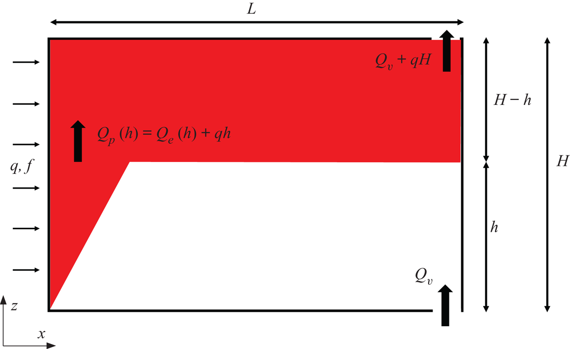
Figure 2. Schematic of the ventilated distributed wall-source plume with a finite source volume flux, where the box is connected to the exterior environment by an open vent at the bottom of the box and a gear pump (not shown) is forcing ventilation by extraction of fluid through openings at the top.
We present results of the ventilated box in the presence of a distributed wall-source plume and apply the theory of Gladstone & Woods (Reference Gladstone and Woods2014) to our results. We first describe the experimental set-up used to perform the experiments.
3. Experimental details
In order to create an unventilated filling box and a ventilated emptying–filling box of a distributed wall-source plume, we enclosed the porous plate described in Part 1 in a Perspex acrylic box with height  $H$ and length $L$,
$L$,  $0.48\ \textrm {m} \times 0.50\ \textrm {m}$, and spanwise length $0.23\ \textrm {m}$ (see figure 3). This was placed inside a Perspex acrylic tank of horizontal cross-section $1.20\ \textrm {m} \times 0.40\ \textrm {m}$ filled up to a depth of $0.75\ \textrm {m}$ with fresh water of density $\rho _a$. The end wall (see the left-hand end of figure 3) of the box had rectangular openings at the top of the wall which allowed an exchange flow to the exterior. Seven valves were connected at the bottom of the end wall which could be closed for a filling box experiment or connected to a pump for the emptying–filling box experiments. In order to force a ventilation flow for the ventilated experiments a gear pump (ISMATEC BVP-Z) was used. Source fluid of density $\rho _s$ was pumped through the wall using a gear pump (Cole-Parmer Digital Gear Pump System, $0.91\ \textrm {ml} \ \textrm {rev}^{-1}$) at a volume flux per unit area of $q$ resulting in a source buoyancy flux of $q(b_s-b_e)$. The formulation of (2.5) assumed a uniform source buoyancy flux per unit area, $f$. Since both the source density and volume flux are constant the source buoyancy flux will not be uniform in the stratified region. Throughout this paper we make the approximation that the source buoyancy flux is given by the constant value of $f=qb_s$, so that the true source buoyancy flux, $\tilde {f}$, is given by $\tilde {f}(z)=f-qb_e(z)$. Although the source volume flux appears in this relation, the error in the formulation of uniform buoyancy flux in our stratified experiments is analogous to the error in the assumption of a uniform heat flux resulting from a isothermal wall within a stratified environment (Caudwell et al. Reference Caudwell, Flór and Negretti2016). We discuss the impact this may have on our results in §§ 4.1 and 4.2 for the filling box and emptying–filling box, respectively. Dye attenuation was used in order to measure the ambient buoyancy stratification. This method is described in detail in § 3.1.
Figure 3. Diagram of the apparatus used to study (a) the filling box and (b) the ventilated box. The openings at the bottom of the tank may be open or closed using a series of valves. Note that the orientation of the experiments is opposite to the model presented in § 2.2. Since density differences are small and the Boussinesq approximation is valid, this change in orientation is not dynamically important i.e. the negatively buoyant plume in the experiments faithfully represents the positively buoyant plume in the model but reversed in direction.
The experimental parameters of the unventilated box and ventilated experiments are shown in table 1. The ventilation flux  $Q_v$ in table 1 is defined as the difference between the physical flux pumped out at the base of the tank and the total source volume flux $qH$. The ratio of the ventilation flux to the maximum theoretical volume flux of the plume, i.e. at $z=H$ in an unstratified environment, is defined by $\psi =Q_v/Q_e(H)$, where $Q_e(H)$ was calculated using the ideal plume solution of the volume flux with the entrainment value $\alpha =0.068$ and skin friction coefficient $C=0.15$ both determined in Part 1.
Table 1. Experimental parameters of the filling box (experiment  $1$) and the ventilated experiments (experiments $2$–
$2$– $12$). The last column, $\psi =Q_v/Q_e(H)$, shows the ratio of the ventilation flow rate compared to the theoretical maximum volume flux of the plume in an unstratified environment. In experiment $12$, blue dye was added to the source solution once the ambient had reached steady state in order to assess the motion of the stratified ambient.
3.1. Dye attenuation
While planar laser-induced fluorescence (LIF) can produce high fidelity density measurements, the technique is limited to examining relatively short experiments, or to be more precise, experiments where a given fluid parcel with fluorescence dye tracer remains in the laser sheet for a relatively short time. This is due to photobleaching of the dye which can occur for longer laser exposures and has a significant effect on the light emissivity of the dye (Crimaldi Reference Crimaldi1997). Given the time scale of a typical filling box or ventilated experiment ( ${\sim }10\text {--}60\ \textrm {min}$), LIF was not a suitable technique to use in order to measure the density field. Instead we used dye attenuation.
Dye attenuation was performed by illuminating the tank from behind using an LED light bank, as shown in figure 4, and measuring the attenuation of light, due to added tracer dye in the source solution, as it passed through the fluid. The Bouguer–Lambert–Beer law may then be used to deduce the integrated concentration of dye along the light path (Cenedese & Dalziel Reference Cenedese and Dalziel1998). The LED light bank was composed of uniformly spaced LEDs with a light diffuser placed between the tank and the array of LEDs. This created a uniform background distribution of light for the experiments. Further, the light bank was driven by a DC power supply which eliminates the pulsing observed with fluorescent lighting for which the frequency of fluctuations in light intensity of the light bank, due to the power supply, affect the images recorded by the camera. The experiments were captured using an AVT Bonito CMC-4000 4 megapixel CMOS camera with a  $80\text {--}200\ \textrm {mm}$ f2.8 Nikon lens at a frame rate of $1\ \textrm {Hz}$ which allowed 200 min of recording time. The camera intensity response was linear with a black offset of $I_b=0.0029$. The resolution of the images was $0.37\ \textrm {mm} \ \textrm {pixel}^{-1}$, however, parallax errors result in a spatially dependent measurement resolution. Away from the horizontal plane of the camera, light has a vertical component in its travel from the light bank to the camera. As such, while passing from the back of the tank to the front (0.25 m) a particular light path will pass through fluid sitting at a range of heights within the tank – thus any measurements inferred from the intensity along a light path represent an average of the fluid properties over those heights. This measurement resolution can be estimated by approximating the camera as a point, at the mid height of the plate, at a distance $10\ \textrm {m}$ from the experimental tank. Simple geometry results in a measurement resolution that varies between $0.37\ \textrm {mm} \ \textrm {pixel}^{-1}$ (owing to the camera resolution) at the mid height of the tank and $6.00\ \textrm {mm} \ \textrm {pixel}^{-1}$ at the top and bottom of the tank. We note that similar considerations apply in the horizontal direction but, since for our measurements horizontal variations are small compared with vertical variations and we average horizontally, these are of no consequence to our experimental results.
Figure 4. Diagram of the experimental set-up used to perform dye attenuation of the filling box and ventilated experiments showing the (a) LED light bank, (b) light diffuser, (c) large reservoir tank and (d) apparatus illustrated in figure 3. The dashed lines indicate the measuring window of the camera which is placed  $10\ \textrm {m}$ from the edge of the large reservoir to minimise the parallax error.
The dye used was red food colouring ‘Fiesta Red’ (Allura Red AC, E129). The molecular diffusivities of the dye and salts ( $\kappa \sim 10^{-9}\ \textrm {m}^2 \ \textrm {s}^{-1}$) are comparable and both a few orders of magnitude lower than the kinematic viscosity of the salt solutions ( $\nu \sim 10^{-6}\ \textrm {m}^2 \ \textrm {s}^{-1}$) so that the dye acts as an effective tracer for the salt concentration. This dye has shown to be effective in previous dye attenuation investigations (e.g. Cenedese & Dalziel Reference Cenedese and Dalziel1998; Coomaraswamy & Caulfield Reference Coomaraswamy and Caulfield2011). The experiments were assumed to be independent of the spanwise $y$-direction, so in order to determine the height dependent profile the light rays should follow horizontal paths. In order to minimise the parallax error, within the constraints of the equipment and the laboratory, the camera was placed $10\ \textrm {m}$ from the experiment. Since the dye acts as a tracer for the sodium chloride solution, the attenuation due to the sodium chloride must also be accounted for.
The depth-integrated view of the camera results in a camera intensity reading of  $I(x,z)$. The Bouguer–Lambert–Beer law may be used to relate a background reference intensity reading $I_0(x,z)$, where the tank contains only fresh water, to the intensity reading with known concentrations of dye and sodium chloride as
 \begin{equation} I(x,z)=I_0(x,z)\exp{(-(\epsilon_{d}c_{d}+\epsilon_{sc}c_{sc})L_{y})}, \end{equation}
where  $\epsilon _{d}$, $\epsilon _{sc}$ and $c_{d}$, $c_{sc}$ are the extinction coefficients and concentrations of the dye and sodium chloride, respectively, and $L_{y}$ is the total distance traversed by the light path through the dyed fluid. In practice, a batch solution of sodium chloride and dye was made so that the relative concentrations of sodium chloride and dye remained constant, i.e. $c_{sc}/c_{d}=\mathcal {C}$. Equation (3.1) may therefore by rewritten in terms of $\mathcal {C}$ and the dye concentration,
 \begin{equation} I(x,z)=I_0(x,z)\exp{(-(\epsilon_{d}+\epsilon_{sc}\mathcal{C})c_dL_{y})}, \end{equation}
where the constant  $\epsilon _{d}+\epsilon _{sc}\mathcal {C}$ was determined empirically by a calibration.
The calibration was performed by filling the tank with a uniform concentration of the batch solution and recording  $200$ images of the field of view. The images were then time averaged to give an intensity reading, for each camera pixel, for a given dye concentration which is used as a proxy for both the dye and sodium chloride concentration. A spatial-averaged normalised pixel intensity reading $\tilde {I}$ was calculated for each concentration from the following
 \begin{equation} \tilde{I}=\frac{1}{A}\int_A\frac{I(x,z)-I_b}{I_0(x,z)-I_b}\,\mathrm{d} x\,\mathrm{d} z, \end{equation}
where  $A$ is the area of the spatial-averaged region and $I_b$ is the camera black offset. In performing the calibration, it was convenient to normalise the dye concentration by the source dye concentration $c_{d,0}$ used in the experiments. The data are plotted in figure 5, which shows an approximately linear relationship between $\log {\tilde {I}}$ and $c_d/c_{d,0}$. The relationship is, however, more accurately fitted by a quadratic curve. The following relationship was found to provide a least squares quadratic best fit
 \begin{equation} \frac{c_d}{c_{d,0}}=0.487\left(\log{\tilde{I}}\right)^2-0.256\log{\tilde{I}}. \end{equation}
It should be noted, however, that the maximum concentration measurements in the region of interest of the experiments, i.e. ignoring regions containing a thin layer of very dense fluid which could not be effectively pumped out by the ventilation, corresponded to a concentration of  $c_d<0.5c_{d,0}$. There is a good linear relationship between $\log {\tilde {I}}$ and $c_d/c_{d,0}$ for this range with a linear best fit of
 \begin{equation} \frac{c_d}{c_{d,0}}=-2.39\log{\tilde{I}}. \end{equation}
Figure 5. Dye attenuation calibration curve for the food colouring dye. The spatial-averaged normalised pixel intensity reading against the normalised dye concentration on a (a) linear–linear axis and a (b) log–linear axis. A linear relationship may be approximately observed in (b), however, a best-fit quadratic curve was used to provide a more accurate relationship. The solid curves correspond to a least squares quadratic fit for  $c_d/c_{d,0}$ in $\log {\tilde {I}}$, where $c_d/c_{d,0}=0.487(\log {\tilde {I}})^2-0.256\log {\tilde {I}}$. The red dashed curves correspond to a least squares linear fit for the data points within the region $0<c_d/c_{d,0}<0.5$ for $c_d/c_{d,0}$ in $\log {\tilde {I}}$, where $c_d/c_{d,0}=-0.239\log {\tilde {I}}$. All concentration measurements in the experiments were within this range.
4. Results
For convenience, the experiments were performed using a relatively dense source solution so that the convention is vertically opposite relative to the theory presented in §§ 2.1 and 2.2, i.e. in the experiments the plume descends and the first front rises whereas in the theory described the plume rises and the first front descends (figure 3a,b). We, therefore, vertically invert the experimental images in order to maintain an analogy between our experiments and a heated room (figures 1 and 2). Since the relative density differences in the experiments and the full scale flows are small, the Boussinesq approximation is valid and the inverted problems are equivalent. Therefore,  $z=0$ and $\xi =0$ are at the top of the experimental tank and the bottom of the filling box, while $z=H$ and $\xi =1$ are at the bottom of the experimental tank but top of the filling box.
4.1. Filling box experiment
4.1.1. First front
We first consider the evolution of the first front of the filling box which has been used to determine the entrainment coefficient in previous studies. Kaye & Cooper (Reference Kaye and Cooper2018) showed that, by ignoring the shear stress and source volume flux when applying the first front theory of Baines & Turner (Reference Baines and Turner1969), artificially low entrainment values are calculated. We show that it is also important to restrict attention to the evolution of the first front in the region where the plume is fully developed.
The height of the first front for each image was calculated by first spatially averaging the processed experimental images of the buoyancy field in the ambient fluid over the range  $0.20\ \textrm {m} < x < 0.45\ \textrm {m}$ so that the plume structure was not included in the spatial average. The standard deviation $\sigma$ across this region was calculated for a background buoyancy field image with no dye added and a threshold of $b_t=10\sigma$ was used to identify the interface. A typical ambient buoyancy profile taken from the filling box experiment is shown in figure 6(a) and the same profile with a logarithmic scale also showing the buoyancy threshold in figure 6(b). The identified position of the interface was insensitive to the choice of threshold, in particular using a threshold of $b_t=5\sigma$ and $b_t=15\sigma$, also shown in figure 6(b), resulted in a mean difference in the identified interface height of $1.2$ and $1.3$ pixels, respectively.

Figure 6. (a) Ambient buoyancy profile of the filling box experiment. (b) The same data presented with a logarithmic buoyancy scale. The vertical dashed line shows the threshold  $b=b_t=10\sigma$ used to identify the first front interface, where $\sigma$ is the standard deviation of the ambient buoyancy from an undyed background image. The other two lines show $b=0.5b_t$ and $b=1.5b_t$.
Figure 7(a) shows the experimentally measured first front against non-dimensional time. Also plotted are three different first front models (FFM) used to predict the position of the first front. These were predicted by assuming that the plume volume flux follows:
(i) the ideal plume solution and the first front descends according to (2.1) with zero source flux;
(ii) the finite-flux plume solution determined by numerically solving (2.3)–(2.5) for $N=0$, which was performed in Part 1 of this work, and the first front descends according to (2.1) with the source flux included; and
(iii) experimental observations using measurements determined in Part 1 of this work and the first front descends according to (2.1) with the source flux included.

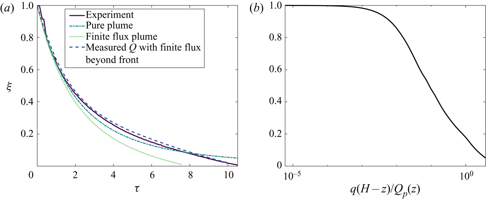
Figure 7. (a) Comparison of the predictions of the position of the first front with experiment  $1$ (solid) for the first front models (FFM) (i) (dot-dashed), FFM (ii) (dotted) and FFM (iii) (dashed) discussed in the text. An entrainment coefficient of $\alpha =0.068$, determined in Part 1, has been used for all the plots. (b) The ratio of the source to plume volume flux contribution to first front movement. The volume flux used in (b) is determined from the velocity measurements over the whole height of the wall measured in Part 1.
Following Kaye & Cooper (Reference Kaye and Cooper2018), (2.1) was numerically integrated to obtain the first front position in FFM (ii) and (iii).
Both the plume volume flux crossing the first front and the additional source volume flux within the stratified region contribute to the rate of descent of the first front. Figure 7(a) shows that all three of the models are successful in predicting the first front position for the region  $\xi >0.6$. In particular, without accounting for the source volume flux in the stratified region, the ideal plume model shows good agreement for $\xi >0.6$. This implies that, even in this region, the contribution of the source volume flux within the stratified region is relatively small compared to the plume volume flux entering the stratified region at the height of the first front. Figure 7(b) shows the relative contributions of the source volume flux to the plume volume flux in the rate of descent of the first front for a given height. The plume volume flux used in this calculation was taken from the velocity measurements over the whole height of the wall performed in Part 1 of this work. This shows that the contribution of the source volume flux to the first front movement is less than $5\,\%$ of the plume volume flux crossing the first front for the region $\xi >0.6$.
The inclusion of the source volume flux in the stratified region of the ideal plume model (FFM (i), marked by the dotted curve) increases the rate of descent of the first front. The experimentally measured first front, however, descends at a slower rate than the ideal plume model with zero source flux (FFM (ii), marked by the dashed-dotted curve). This can be explained using the velocity measurements over the whole height of the wall, where a laminar region was observed for  $\xi <0.15$. Beyond this, the plume was not fully developed within the region $\xi <0.6$ so the ideal plume model did not provide an accurate prediction of the volume flux within this region.
Figure 7(a) shows that the first front position may be successfully predicted for the entire descent by including the volume flux measurements in the first front equation and including the contribution of source volume flux in the model (FFM (iii), marked by the dashed curve). This is the first time such accurate predictions have been achieved.
The different models demonstrate the importance of accounting for the laminar region of the flow in predicting the first front descent. Caudwell et al. (Reference Caudwell, Flór and Negretti2016) accounted for this by using a hybrid model whereby the laminar region is modelled using the similarity solutions presented by Worster & Leitch (Reference Worster and Leitch1985) and the turbulent region is modelled using pure plume theory for the turbulent zone with constant entrainment coefficient. The hybrid model resulted in a slower rate of descent, compared to a pure plume model, similar to the observation that FFM (iii) results in a slower descent compared to FFM (ii). However, compared to experimental observations, the hybrid model resulted in larger disagreement than their pure plume model, whereas our FFM (iii) results in an improved agreement compared to the pure plume model. Caudwell et al. (Reference Caudwell, Flór and Negretti2016) also considered another type of hybrid model where a time-dependent entrainment coefficient, determined from calculating the height-averaged entrainment coefficient in a filling box experiment, was incorporated into the original hybrid model. The first front descent of this model showed improved agreement to experimental observations, albeit with notable discrepancies near the base of the tank which suggests that the volume flux of the laminar region was not effectively modelled.
4.1.2. Ambient stratification
Figure 8(a) shows the time evolution of the ambient buoyancy where the position of the first front has been overlayed. Figure 8(b) shows the buoyancy profiles for selected times. Within the region  $\xi <0.95$ the horizontal buoyancy averages resulted in an average standard deviation, across all heights, of less than $5\,\%$ providing an estimate of the uncertainties within our measurements. The variation was larger near the base of the tank owing to the gravity current that formed. The profiles are qualitatively similar to those of Caudwell et al. (Reference Caudwell, Flór and Negretti2016) and Bonnebaigt et al. (Reference Bonnebaigt, Caulfield and Linden2018), i.e. they include a sharp tail of rapidly decreasing buoyancy from the top of the box to an approximately linear region, followed by an increase in $N^2$ close to the first front. Cooper & Hunt (Reference Cooper and Hunt2010) did not present results of the filling box ambient buoyancy profiles and so this comparison with their work is not possible.

Figure 8. (a) The time evolution of the spatial-averaged ambient density field for the filling box experiment  $1$ (see table 1) and (b) the spatial-averaged ambient density profiles for non-dimensional time $\tau = 1,\ldots ,10$. The dashed curve in (a) shows the position of the first front.
We now consider the filling box peeling model based on the work of Bonnebaigt et al. (Reference Bonnebaigt, Caulfield and Linden2018) discussed in § 2.1 and compare the model to the experimental results. We consider three different filling box models (FBM). First, FBM (i), we consider the ideal plume solutions (Part 1 (2.19)–(2.21)), using the experimentally determined entrainment and skin friction coefficient. The position of the first front is then determined analytically by (2.2). In this model, as in Bonnebaigt et al. (Reference Bonnebaigt, Caulfield and Linden2018), linear plume velocity and buoyancy profiles are assumed as defined in (2.9a,b), which gives a cumulative buoyancy distribution of volume flux as defined in (2.10). This model only differs to that of Bonnebaigt et al. (Reference Bonnebaigt, Caulfield and Linden2018) by the inclusion of a skin friction coefficient.
In the second model, FBM (ii), the ideal plume solutions are again used to calculate the volume flux entering the stratified region. The difference here, however, is that the cumulative buoyancy distribution of volume flux imposed at the first front was experimentally determined by conditionally averaging the simultaneous velocity and buoyancy data measured in Part 1. The cumulative buoyancy distribution of volume flux was determined from the data by the following calculation
 \begin{equation} Q_{b}(b^*,z)=\frac{1}{T}\int_0^{T}\int_0^{\infty}w(x,z,t)\mathscr{H}(b(x,z,t)-b^*)\,\mathrm{d} x\,\mathrm{d} t, \end{equation}
where  $\mathscr {H}$ is the Heaviside step function and $T$ is the total recording time. The mean cumulative buoyancy distribution of volume flux is shown in figure 9 (black) scaled by the total volume flux where the buoyancy is scaled by the characteristic buoyancy, defined by $b_T=F/Q_p$. The curve shows the average, across all heights measured, of the scaled data. For each height, the standard deviation, over the four experiments, of the averaged curves varied between $2\,\%$ and $5\,\%$, with larger standard deviation between experiments for large buoyancy reflecting the difficulty measuring both the buoyancy and velocities close to the wall. The cumulative distribution function assumed by Bonnebaigt et al. (Reference Bonnebaigt, Caulfield and Linden2018) (blue) and the result of assuming an integral (i.e. top-hat) profile (dashed) are also shown in figure 9. The maximum buoyancy predicted by the model of Bonnebaigt et al. (Reference Bonnebaigt, Caulfield and Linden2018) is $b_m=1.5b_T$. The experimental data (black) show that there is a large transport of buoyant fluid, approximately $25\,\%$ of the total transport, which is greater than the maximum buoyancy predicted by the model of Bonnebaigt et al. (Reference Bonnebaigt, Caulfield and Linden2018).
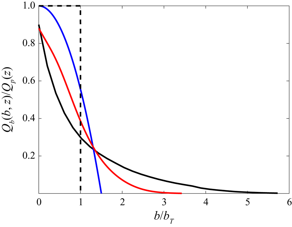
Figure 9. The cumulative buoyancy distribution of volume flux for the distributed wall-source plume in an unstratified environment (black) calculated using the simultaneous velocity and buoyancy data from Part 1. Also shown is the cumulative buoyancy distribution of volume flux used by Bonnebaigt et al. (Reference Bonnebaigt, Caulfield and Linden2018) (blue), the resulting distribution from assuming a top-hat velocity and buoyancy profile (dashed) and the distribution of a wall plume resulting from a horizontal line-source of buoyancy adjacent to a wall (red), calculated from the data presented in Parker et al. (Reference Parker, Burridge, Partridge and Linden2020). The buoyancy has been scaled by the characteristic plume buoyancy  $b_T$, where for the wall plume $b_T=F_0/Q_p$ with source buoyancy flux $F_0$.
Figure 9 shows that, for the experimental data,  $Q_{b}(0,z)<Q_p(z)$. This is due to the vertical transport of ambient fluid by the distributed wall-source plume, which is equal to $Q_p(z)-Q_{b}(0,z)$. Significant vertical transport of ambient fluid has also been observed in both axisymmetric (Burridge et al. Reference Burridge, Parker, Kruger, Partridge and Linden2017), wall and free line plumes (Parker et al. Reference Parker, Burridge, Partridge and Linden2020). The plume, therefore, transports (unmixed) ambient fluid into the stratified region. The peeling model assumes that the plume fluid peels to its neutral buoyancy height. The neutral buoyancy height of the transported unmixed ambient fluid would be below the stratified region, so in order to match the plume volume flux with the descending first front we assume that the transported ambient fluid is mixed into the stratified region. To parameterise this mixing, and in order to use the experimental cumulative distribution function in the peeling model, we first rescale the experimental data $Q_{b}(b^*,z)$ by the volume flux of plume fluid $Q_{b}(0,z)$. The buoyancy is then rescaled in order to conserve buoyancy flux so that the following relation holds
 \begin{equation} \frac{1}{b_TQ_p(z)}\int_0^{\infty}Q_{b}(b^*,z)db^*=1. \end{equation}
The third model, FBM (iii), uses FFM (iii) to predict the position of the first front. The peeling procedure discussed for FBM (ii) is then used to determine the ambient density profile.
Figure 10 shows the results of the three peeling models described and compares them against the experimental data. The first front descent is identical in FBM (i) and FBM (ii). FBM (ii), however, is able to predict the buoyancy gradient of the approximately linear region observed in experiments. FBM (i) underestimates the buoyancy observed in the experiments within the region  $\xi >0.75$ and vice versa, suggesting that the linear velocity and buoyancy profiles overestimate the mixing that occurs within the plume. In contrast, FBM (ii) overestimates the buoyancy observed in the region $\xi >0.75$, which is to be expected since the cumulative buoyancy distribution of volume flux has been imposed from direct measurements in an unstratified environment and no further mixing is assumed as the plume enters the stratified region. FBM (iii), which follows the first front position more accurately by using FFM (iii), does not show significant improvement over FBM (ii).
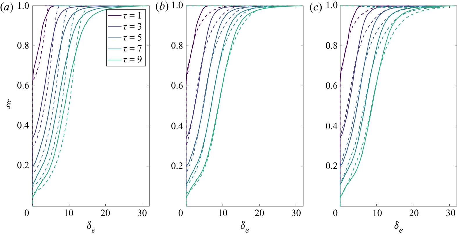
Figure 10. Comparison of the filling box peeling models (dashed curves) compared with experiment  $1$ (solid curves) for non-dimensional times $\tau =1,3,5,7$ and 9 for (a) FBM (i), (b) FBM (ii) and (c) FBM (iii) discussed in the text.
The results above suggest that it is possible to modify the experimentally determined cumulative buoyancy-distribution function, which could be thought of as a mixing parameterisation of the plume entering the stratified region, so that the peeling model more accurately describes the observed buoyancy profiles within the ambient. It is expected, however, that the cumulative buoyancy distribution is not self-similar in the developing, and especially, the laminar region of our experiment.
Figure 9 also shows the cumulative buoyancy distribution of volume flux of a wall plume calculated from the data presented in Parker et al. (Reference Parker, Burridge, Partridge and Linden2020). It is clear that, relative to the characteristic plume buoyancy, the distributed wall-source plume exhibits a greater range of buoyancy than the wall plume. This is due to the continued supply of buoyant fluid at the wall as well as the ongoing mixing of ambient fluid within the stratified region. Bonnebaigt et al. (Reference Bonnebaigt, Caulfield and Linden2018) also examined the filling box in the presence of a horizontal line source adjacent to a wall, where the top-hat model of Germeles (Reference Germeles1975) was shown to accurately predict the developing buoyancy stratification.
Relative to the source buoyancy ( $\delta _s=35.8$), the buoyancy of the ambient environment can be significant and vary with height. However, this does not affect the peeling method which depends only on the buoyancy profile in the plume at the height of the first front, and does not depend on capturing the dynamics of the plume within the stratified region. Moreover, the addition of buoyancy within the stratified region, which results from the addition of uniform density fluid from the source, is properly accounted for within our modelling (§ 2). Therefore, the comparison between the experimental results and the model is not affected by the source buoyancy flux varying with height within the stratified region.
4.2. Ventilated experiments
We first examine the steady-state interface height of the ventilated experiments. Following Baines (Reference Baines1983) and Gladstone & Woods (Reference Gladstone and Woods2014), the height of the steady-state interface  $h_i$ (or $\xi _i$ in non-dimensional form) was measured from experiments and the interface height was predicted by assuming that the ventilation flow rate $Q_v$ matches the volume flux of the plume at the height of the interface (Baines Reference Baines1983). Therefore
 \begin{equation} Q_v=Q_p(h_i)-qh_i=Q_e(h_i). \end{equation}
By assuming that the cumulative entrained volume flux follows the ideal plume volume flux solution determined in Part 1, (4.3) may be used to express the interface height in terms of the ventilation flow rate as
 \begin{equation} \frac{h_i}{H}=\left(\frac{4Q_v}{3}\right)^{3/4}\left(\frac{4\alpha^2fH^4}{5}\right)^{-1/4}\left(1+\frac{4C}{5\alpha}\right)^{1/4}=\psi^{3/4},\end{equation}
where we recall that  $\psi =Q_v/Q_e(H)$ is the ratio of the ventilation rate to the plume volume flux. We also predict the height of the interface using the results of the velocity measurements over the whole height of the wall in Part 1. According to this model, the interface height is given by $h_i=Q_e^{-1}(Q_v)$, where $Q_e^{-1}$ is the inverse relationship of the average of the experimental data shown in Part 1 figure $6$(b). Figure 11(a) shows the predicted interface heights for both models discussed above compared with the measured interface heights from the experiments. Figure 11(b) shows a typical evolution of the ambient stratification in a ventilated experiment, as it ultimately reaches steady state.

Figure 11. (a) Comparison of the predicted steady-state interface heights for the two models considered in the text with the measured interface height from the experiments. (b) An example of the evolution of the ambient buoyancy profile, taken from experiment  $5$, as it tends to a steady state.
Figure 11(a) shows that the ideal plume model (red) is able to predict the interface height reasonably well for the region  $\xi >0.58$. This is consistent with the observation that the ideal plume model is also able to accurately predict the first front height of the filling box model within this region. The ideal plume model predictions, however, become increasingly poor as the interface height decreases, i.e. as the ventilation flow ratio $\psi$ decreases. As in the case of the first front model FFM (i), the inaccuracy arises because the plume is not fully developed in the lower region. The model is improved by incorporating volume flux measurements over the whole height of the wall (black diamonds), where the interface heights for the low ventilation flow rates are accurately predicted.
Figure 12 shows the steady-state buoyancy profiles across all the ventilated experiments. The buoyancy profiles are qualitatively similar to those observed by Cooper & Hunt (Reference Cooper and Hunt2010) and Gladstone & Woods (Reference Gladstone and Woods2014) where for low ventilation flow rates they follow an S-shaped curve in which the buoyancy rapidly increases from the interface height towards an approximately linear region, and for relatively high ventilation flow rates the buoyancy increases linearly away from the interface. Beyond this there exists a relatively well-mixed region, for example the region  $0.85<\xi <0.90$ for $\psi =0.439$, and then a region of rapidly increasing buoyancy. The well-mixed region is a result of the gravity current formed at the base of the tank (i.e. at the top in the orientation presented in figure 12), and the rapidly increasing buoyancy may be a result of the position of the ventilation openings at the far wall, as opposed to Cooper & Hunt (Reference Cooper and Hunt2010) where the ventilation openings were along the base of the box. An interface, separating the gravity current at the base of the tank and the approximately linear ambient buoyancy, at approximately $\xi =0.85$ can be observed in each of the experiments in figure 12.

Figure 12. Steady-state ambient buoyancy profiles of the ventilated experiments. The data points shown are sub-sampled at a resolution of  $\Delta \xi =0.011$ to aid clarity to the figure. This corresponds to the resolution at a height of $\xi =0.90$.
In order to identify the dynamics of the ambient fluid within the stratified region, relatively concentrated blue dye was added to the source solution in experiment  $12$ after steady state had been achieved. To perform analysis on the data it was convenient to study the raw experimental images. A time average of the experiment during steady state, before any blue dye had been added, was used as a background image in order to aid clarity to the motion of the dye (figure 13a). Figure 13(b) shows an instantaneous image of the experiment $40$ min ( $\tau =18.2$) after the blue dye had been added to the source. Figure 13(c) has been normalised by the background image shown in 13(a). A supplementary movie of the full duration of the experiment is available at https://doi.org/10.1017/jfm.2020.809. The movie has been corrected, equivalent to figure 13(c).

Figure 13. (a) Time average of the raw experimental images recorded during the steady state before the blue dye had been added to the source solution. (b) Raw experimental image of the experiment 40 min ( $\tau =18.2$) after the blue dye had been added to the source solution. (c) Corrected image where the image from (a) is subtracted from (b). The area in between the blue lines in (c) shows the region used to vertically average the image in order to identify the mean horizontal motion of the dye into the ambient (figure 14). Similarly, the area the between the red lines shows the region used to horizontally average the image in order to identify the mean vertical motion of the dye into the ambient. The dashed line shows the height of the steady-state interface and the dotted line shows the characteristic plume width, $R =\alpha z$, using the value $\alpha =0.068$ determined from Part 1.
For each experimental frame, after the blue dye had been added to the source, horizontal and vertical spatial averages were performed in the regions shown between the vertical red and horizontal blue lines in figure 13(c), respectively. The mean vertical and horizontal motion of the dye within the stratified region could then be assessed over time. Figure 13(c) shows that there is a region within the stratified zone, approximately  $x<0.20\ \textrm {m}$, where the dyed source fluid has entered the ambient region. This structure developed shortly after the dye had been added, however, it remained bounded within this region and did not spread further into the ambient fluid. The region used to identify the mean vertical motion was therefore placed outside of the structure identified from the dye. Similarly, the region used to identify the horizontal motion was placed outside the gravity current, which can be seen at the top of the figure in 13(c). The evolution of the dye within the regions highlighted between the red and blue lines in figure 13(c) are shown in figure 14. The flushing time of the source chamber is approximately $10$ min for the source flow rate used. Therefore, the source solution gradually becomes more concentrated until reaching a uniform dye concentration. The effect of this can be observed in figures 14(a) and 14(b), where the dye concentration gradually increases. Figure 14(a) shows the vertical motion of the dye. The dye clearly shows the vertical extent of the gravity current at the base of the tank. The maximum height of the dye remains approximately constant after $20$ min ( $\tau =9.1$), and the deviation in the maximum height is estimated to be $5\ \textrm {mm}$ for the remainder of the experiment. Any vertical intrusion of the dye into the ambient is therefore estimated to occur at a speed of less than $2.5 \times 10^{-3}\ \textrm {mm} \ \textrm {s}^{-1}$ which corresponds to $0.02Q_v/L$. Further, the effects of diffusion, of both the salt and dye, may be neglected given the low diffusivities (the diffusion length for a time scale of 40 min is ${\sim }5\ \textrm {mm})$.
Figure 14(b) shows the horizontal motion of the dye. The figure suggests that there is a mixing zone in the region  $x<0.20\ \textrm {m}$, which can also be seen in figure 13(c), since the dyed source fluid rapidly replaces any un-dyed source fluid within this zone. The (horizontal) width of this mixing zone was not uniform across the spanwise $y$-direction. This is highlighted in the figure by the labels where separate intrusions at different $y$ locations occurred. These can be distinguished from the regions of blue and green. The blue region is an intrusion that exists closer to the camera and the green intrusion exists behind the blue region so that only the furthest point away from the wall is visible. As the depth of intrusion A (green) increases, the depth of intrusion B (blue) decreases, which suggests that there is an approximate conservation of total volume within the mixed region and the entrainment and peeling balance, as can also be observed in the supplementary movie. Similar results were observed by Gladstone & Woods (Reference Gladstone and Woods2014). There is, however, a continued supply of source fluid within this region, so we hypothesise that within this region the time-average plume volume flux is given by ${Q_p(z)=Q_v+qz}$. Based on this assumption we may adapt the theory developed by Gladstone & Woods (Reference Gladstone and Woods2014) for a vertically distributed line-source plume to a distributed wall-source plume.
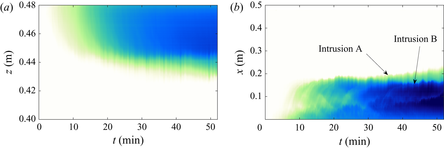
Figure 14. (a) Horizontally and (b) vertically spatial-averaged evolution of the blue dye added to the source solution. The regions used to spatial average are shown in figure 13(c). The figures suggest that there is no net vertical motion within the stratified ambient region  $0.20\ \textrm {m} < x < 0.50\ \textrm {m}, h_i < z < 0.42\ \textrm {m}$.
As discussed in § 2.2, Gladstone & Woods (Reference Gladstone and Woods2014) suggested that the absence of any vertical transport within the ambient implies that there is a buoyancy difference  $\Delta b$ between the mean plume and ambient density within the stratified region which serves to maintain the vertical motion of the plume. Since the system is in steady state this buoyancy difference should remain independent of depth.The characteristic plume buoyancy in the unstratified region is given by
 \begin{equation} b_T=\frac{f z}{Q_p}=\frac{4}{3}\left(\frac{5}{4}\right)^{1/3}\alpha^{-2/3}f^{2/3}\left(1+\frac{4C}{5\alpha}\right)^{1/3}z^{-1/3}.\end{equation}
In the stratified region, assuming that the volume flux is given by  $Q_p(z)=Q_v+qz$, the characteristic plume buoyancy is given by
 \begin{equation} b_T=\frac{f z}{Q_v+qz}. \end{equation}
If the source volume flux is ignored, the linear growth rate of plume buoyancy is recovered as derived by Gladstone & Woods (Reference Gladstone and Woods2014). Figure 15(a) shows the model prediction for experiment  $3$ compared to the experimental steady-state buoyancy profile. Note the nonlinear profile of the model characteristic plume buoyancy, which qualitatively follows the ambient buoyancy.
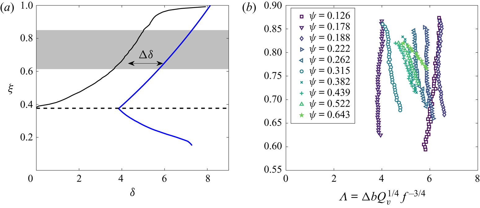
Figure 15. (a) The steady-state ventilation model (4.5) and (4.6) (blue), which has been adapted from the model of Gladstone & Woods (Reference Gladstone and Woods2014), compared to experiment  $3$ (black). The dashed line shows the height of the interface. The height-invariant buoyancy difference $\Delta \delta$ between the plume and ambient fluid, predicted by Gladstone & Woods (Reference Gladstone and Woods2014), is shown in the figure. (b) Normalised buoyancy difference, $\varLambda =\Delta bQ_v^{1/4}f^{-3/4}$ , as a function of height within the stratified core (for example the grey region in (b) for experiment $3$).
$3$).
In order to test whether  $\Delta b$ is independent of depth in the core of the stratified region, the buoyancy difference was calculated as a function of height for each experiment. We define the core of the stratified region as the heights between the gravity current and the mid height between the gravity current and the interface, as highlighted in grey for experiment $3$ in figure 15(a). We again consider only the ambient region away from the mixing zone and walls, as highlighted by the region in between the vertical red lines in figure 13(c). The identification of the interface between the stratified and unstratified region was performed using an identical methodology to that used to identify the first front, described in § 3.1. In order to identify the upper boundary of the stratified core the heights of the inflection points of the steady-state profiles were calculated, i.e. the heights $\xi _g$ such that $\delta ^{\prime \prime }_e(\xi _g)=0$. Given the data were averaged over $0.2\ \textrm {m}$, the profiles did not require further smoothing and the inflection points were clearly identifiable. The gravity current was then defined as the region $\xi >\xi _g$, where $\xi _g$ is the second inflection point moving from $\xi =1$ in the negative $\xi$ direction. Figure 15(b) shows the results, where the buoyancy difference has been normalised using $\varLambda =\Delta bQ_v^{1/4}f^{-3/4}$.
Figure 15(b) shows that the buoyancy difference remains approximately constant for experiments with  $\psi <0.4$. For experiments with $\psi >0.4$ there is a noticeable reduction in the buoyancy difference with increasing height, and in particular $\mathrm{d} \varLambda /\mathrm{d} \xi$ tends to decrease with increasing $\psi$. The stratified region within these experiments is relatively small, especially considering only the stratified core. It may be, therefore, that these experiments are unable to develop a balanced entrainment/peeling region. Further, this trend suggests that the stratification is stronger than the theory predicts for these experiments (i.e. where the stratified zone begins nearer the top of the box), so that the stratification is dominated by the result of matching the large buoyancy near the top of the box to the zero buoyancy at the interface. Gladstone & Woods (Reference Gladstone and Woods2014) suggested that $\varLambda$, or the equivalent non-dimensional constant for a vertically distributed buoyant line-source plume, should be a constant of order unity because the flow is turbulent so the buoyancy difference should depend only the ventilation flow rate and buoyancy flux per unit area. There is no distinguishable trend of the mean value of $\varLambda$ for each experiment as a function of $\psi$, indeed the maximum variation between experiments occurs between experiments with $\psi =0.178$ and $\psi =0.188$. For a distributed wall-source plume we find a value of $\varLambda =5.3\pm 0.8$, which is the mean and standard deviation of the mean value from each experiment.
As discussed in § 3, the source buoyancy flux within the stratified region is not uniform. As the ambient buoyancy increases, the source buoyancy flux decreases. As figure 12 shows, this effect is magnified as the ventilation flow rate is decreased. We draw our conclusions based on the stratified core suggesting that the strongly stratified region above this core does not affect our results. Based on a source buoyancy flux of  $\delta _s=35.8$ the difference between the assumed and true source buoyancy flux varies between a maximum (within each experiment) of $3\,\%$ and $21\,\%$. The decrease in source buoyancy flux with height may also contribute to the deviation from a linear ambient buoyancy profile. This may explain why, for the minimum flow rate (i.e. the maximum decrease in source buoyancy flux), the stratification is weaker than predicted.
5. Application
5.1. Creating a desired linear temperature stratification
In the industrial testing of air movement products it is often desirable to understand the interaction between the product and a known controllable stratification within a room or test chamber. Achieving steady-state ventilation regimes which produce a canonical linear stratification of known buoyancy frequency has been challenging for industrial testing. In this paper we have provided the required modelling and validation in order to resolve this challenge for a wall warmed (or cooled) by a uniform heat flux.
For a ventilated room with a wall of uniform heat flux per unit area, the theory and results presented in this study show that it is possible to create a steady-state regime with an approximately linear ambient temperature stratification where, by suitable choices of the heat flux and the ventilation flow rate, the height of the steady-state interface and the ambient temperature gradient may be controlled independently of one other. Our results suggest that the room would contain an unstratified region of uniform temperature, followed by a gradual increase in temperature to the linearly stratified zone and finally a rapid increase temperature towards the ceiling.
Equations (2.14) and (4.4) imply that a steady-state interface height  $h$ and temperature gradient $\mathrm{d} T/\mathrm{d} z$, i.e. buoyancy frequency $N^2=g\beta \mathrm{d} T/\mathrm{d} z$ (where $\beta$ is the thermal expansion coefficient of the ambient fluid), may be achieved by imposing the following source buoyancy flux per unit area and ventilation flow rate per unit length
 \begin{gather} f=AN^3h^2, \end{gather}
 \begin{gather}Q_v=ANh^2, \end{gather}
respectively, where
 \begin{equation} A^2=\frac{4}{5}\left(\frac{3}{4}\right)^{3}\alpha^2\left(1+\frac{4C}{5\alpha}\right)^{-1}, \end{equation}
with the entrainment coefficient  $\alpha \approx 0.068$ and the wall skin friction coefficient $C\approx 0.15$, as determined in Part 1. The heat flux $q''$ required to achieve the buoyancy flux given by (5.1) may be expressed as (Batchelor Reference Batchelor1954)
 \begin{equation} q''=\frac{f\rho c_p }{g\beta}=\frac{AN^3h^2\rho c_p }{g\beta}, \end{equation}
where  $c_p$ is the specific heat capacity of the ambient fluid. The interface height may be chosen to maximise the linearly stratified region of the test section, keeping in mind that the results presented are only valid for the turbulent regime. Consequently, $h$ should be chosen to be greater than the distance of the transition to turbulence, which is typically less than $z=1\ \textrm {m}$ in the case where the relative wall to ambient fluid temperature $\Delta T>5\ \textrm {K}$.
We consider an example with  $h=1\ \textrm {m}$, an initial ambient temperature of $T_a=20\,^{\circ }\textrm {C}$ and a test section with a temperature gradient of $\mathrm{d} T /\mathrm{d} z =2\ \textrm {K} \ \textrm {m}^{-1}$. For these conditions (5.4) gives a heat flux per unit area of $q''=14.9\ \textrm {W} \ \textrm {m}^{-2}$ and a ventilation flow rate of $Q_v=0.0061\ \textrm {m}^{2} \ \textrm {s}^{-1}$. Using the results from § 4.2 gives that the ambient stratified region follows the temperature profile $T_e$, where
 \begin{equation} T_e-T_a= \left(h\frac{\mathrm{d} T}{\mathrm{d} z}\right)\frac{z}{h}-\frac{\varLambda A^{1/2}N^2h}{g\beta}=\left(\frac{2z}{h}-1.6\right)\ \textrm{K}. \end{equation}
5.2. Heated wall in atrium
Here, we consider the situation where absorbed solar radiation by a glass wall of an atrium results in a significant convective heat flux resulting in a distributed wall-source plume. The typical air quality requirement for room occupancy is  $0.01\ \textrm {m}^{3} \ \textrm {s}^{-1}$ per person where room occupancy density for an atrium is typically in the range $2\text {--}10\ \textrm {m}^2$ per person. This suggests, for a room with length $10\ \textrm {m}$ (in the direction normal to the heated wall), ventilation flow rates between $0.01\ \textrm {m}^{2} \ \textrm {s}^{-1}$ and $0.05\ \textrm {m}^{2} \ \textrm {s}^{-1}$. Figures 16(a) and 16(b) show data spanning these required flow rates and present the resulting ambient temperature gradient and steady-state interface height for varied heat fluxes, $q''$, within the range that would be expected from absorbed solar radiation by glass. The model assumes that other heat gains and losses within the room are negligible compared to the wall-source heat flux.
Figure 16. The (a) ambient temperature gradient and (b) steady-state interface height as functions of the heat flux for selected ventilation flow rates in a typical atrium.
6. Conclusions
By enclosing the distributed wall-source plume, the classical filling box problem was investigated by using dye attenuation to measure the ambient buoyancy field. By adapting the peeling model of Bonnebaigt et al. (Reference Bonnebaigt, Caulfield and Linden2018) to include direct measurements of the cumulative buoyancy distribution of volume flux, the developing buoyancy stratification was successfully predicted.
The emptying–filling box problem was also studied. For a fixed buoyancy flux per unit area the developing buoyancy stratification, and in particular the steady-state profile, was measured for varying ventilation flow rates. In steady state, negligible vertical transport in the stratified ambient was observed suggesting that, as in the case of a vertical line source of buoyancy studied by Gladstone & Woods (Reference Gladstone and Woods2014), there is a balance between the entrainment of the stratified ambient fluid and peeling of plume fluid into the ambient. Based on this observation we adapted the theory developed by Gladstone & Woods (Reference Gladstone and Woods2014) to the present configuration to show that the steady-state ambient buoyancy, within the stratified region, is given by  $b_e=f z/(Q_v+q z)-\Delta b$ and the buoyancy difference can be expressed as $\Delta b=\varLambda f^{3/4}Q_v^{-1/4}$ for some non-dimensional constant $\varLambda$. The buoyancy difference $\Delta b$ was found to be approximately constant within the core of the stratified region for the lower ventilation experiments. On the other hand, for the higher ventilation flow rates there was an obvious trend that $\mathrm{d} \Delta b/\mathrm{d} z<0$. The calculated non-dimensional constant $\varLambda$ was relatively scattered, even across those experiments that followed the theory well, with a value of $\varLambda =5.3\pm 0.8$.
Our conclusions present us with distinct dynamics of the plume which dominates the behaviour within the stratified region: the peeling mechanism during the filling box and the balanced peeling-entrainment mechanism in the steady-state emptying–filling box. While we have not studied the early-time entrainment mechanism of the emptying–filling box, our results do not preclude a dominant peeling mechanism within the transient regime prior to steady state. It should also be noted that a steady-state ambient stratification prohibits anything other than balanced peeling entrainment, since net peeling or net entrainment would modify the stratification away from steady state.
Finally, based on the results presented in this study, we considered two practical examples. Firstly, we suggested a methodology for industrial applications whereby a chosen linear temperature stratification within a room may be achieved with a uniform wall heat flux. Secondly, we considered the situation of practical interest of a large space or atrium where there is a distributed source of heat along one wall, for example solar radiation absorbed at the façade in glazing or interior shading devices.
Acknowledgements
The authors gratefully acknowledge illuminating conversations with Dr T. Jukes regarding the application of this work within industry. We are grateful to the skilled technical staff of the G. K. Batchelor Laboratory for the manufacture of the apparatus and the illumination system. We also wish to acknowledge the contribution of Professor S. Dalziel to the data capture and processing. The work has received financial support from the UK Engineering and Physical Sciences Research Council through an iCASE award with Arup, the First Grant EP/R008957/1 ‘Confinement, boundaries and buoyancy in the mixing by fluid flows’ and also through the Programme Grant EP/K034529/1 ‘Mathematical Underpinnings of Stratified Turbulence’ (MUST), and from the European Research Council through the Horizon 2020 research and innovation programme agreement no. 742480 ‘Stratified turbulence and mixing processes’ (STAMP). The data associated with this paper can be found in the repository https://doi.org/10.17863/CAM.57141.
Declaration of interests
The authors report no conflict of interest.
Supplementary movie
Supplementary movie is available at https://doi.org/10.1017/jfm.2020.809.


 Open access